Student’s t Distribution based Estimation of Distribution Algorithms for Derivative-free Global Optimization

Abstract

In this paper, we are concerned with a branch of evolutionary algorithms termed estimation of distribution (EDA), which has been successfully used to tackle derivative-free global optimization problems. For existent EDA algorithms, it is a common practice to use a Gaussian distribution or a mixture of Gaussian components to represent the statistical property of available promising solutions found so far. Observing that the Student’s t distribution has heavier and longer tails than the Gaussian, which may be beneficial for exploring the solution space, we propose a novel EDA algorithm termed ESTDA, in which the Student’s t distribution, rather than Gaussian, is employed. To address hard multimodal and deceptive problems, we extend ESTDA further by substituting a single Student’s t distribution with a mixture of Student’s t distributions. The resulting algorithm is named as estimation of mixture of Student’s t distribution algorithm (EMSTDA). Both ESTDA and EMSTDA are evaluated through extensive and in-depth numerical experiments using over a dozen of benchmark objective functions. Empirical results demonstrate that the proposed algorithms provide remarkably better performance than their Gaussian counterparts.

derivative-free global optimization, EDA, estimation of distribution, Expectation-Maximization, mixture model, Student’s t distribution

I Introduction

The estimation of distribution algorithm (EDA) is an evolutionary computation (EC) paradigm for tackling derivative-free global optimization problems [1]. EDAs have gained great success and attracted increasing attentions during the last decade [2]. Different from most of EC algorithms which are normally equipped with meta-heuristics inspired selection and variation operations, the EDA paradigm is characterized by its unique variation operation which uses probabilistic models to lead the search towards promising areas of the solution space. The basic assumption is that probabilistic models can be used for learning useful information of the search space from a set of solutions that have already been inspected from the problem structure and this information can be used to conduct more effective search. The EDA paradigm provides a mechanism to take advantage of the correlation structure to drive the search more efficiently. Henceforth, EDAs are able to provide insights about the structure of the search space. For most existent EC algorithms, their notions of variation and selection usually arise from the perspective of Darwinian evolution. These notions offer a direct challenge for quantitative analysis by the existing methods of computer science. In contrast with such meta-heuristics based EC algorithms, EDAs are more theoretically appealing, since a wealth of tools and theories arising from statistics or machine learning can be used for EDA analysis. Convergence results on a class of EDAs have been given in [3].

All existent EDAs fall within the paradigm of model based or learning guided optimization [2]. In this regard, different EDAs can be distinguished by the class of probabilistic models used. An investigation on the boundaries of effectiveness of EDAs shows that the limits of EDAs are mainly imposed by the probabilistic model they rely on. The more complex the model, the greater ability it offers to capture possible interactions among the variables of the problem. However, increasing the complexity of the model usually leads to more computational cost. The EDA paradigm could admit any type of probabilistic model, among which the most popular model class is the Gaussian model. The simplest EDA algorithm just employs univariate Gaussian models, which regard all design variables to be independent with each other [4, 5]. The simplicity of models makes such algorithms easy to implement, while their effectiveness halts when the design variables have strong interdependencies. To get around of this limitation, several multivariate Gaussian based EDAs (Gaussian-EDAs) have been proposed [6, 4, 7]. To represent variable linkages elaborately, Bayesian networks (BNs) are usually adopted in the framework of multivariate Gaussian-EDA, while the learning of the BN structure and parameters can be very time consuming [8, 9]. To handle hard multimodal and deceptive problems in a more appropriate way, Gaussian mixture model (GMM) based EDAs (GMM-EDAs) have also been proposed [10, 11]. It is worthwhile to mention that the more complex the model used, the more likely it encounters model overfitting, which may mislead the search procedure [12].

The Student’s t distribution is symmetric and bell-shaped, like the Gaussian distribution, but has heavier and longer tails, meaning that it is more prone to producing values that fall far from its mean. Its heavier tail property renders the Student’s t distribution a desirable choice to design Bayesian simulation techniques such as the adaptive importance sampling (AIS) algorithms [13, 14, 15]. Despite the purpose of AIS is totally different as compared with EDAs, AIS also falls within the iterative learning and sampling paradigm like EDAs. The Student’s t distribution has also been widely used for robust statistical modeling [16]. Despite of great success achieved in fields of Bayesian simulation and robust modeling, the Student’s t distribution has not yet gained any attention from the EC community.

In this paper, we are concerned with whether the heavier tail property of the Student’s t distribution is beneficial for developing more efficient EDAs. To this end, we derive two Student’s t distribution based algorithms within the paradigm of EDA. They are entitled as estimation of Student’s t distribution algorithm (ESTDA) and estimation of mixture of Student’s t distribution algorithm (EMSTDA), implying the usages of the Student’s t distribution and the mixture of Student’s t distributions, respectively. We evaluate both algorithms using over a dozen of benchmark objective functions. The empirical results demonstrate that they indeed have better performance than their Gaussian counterparts. In literature, the closest to our work here are the posterior exploration based Sequential Monte Carlo (PE-SMC) algorithm [13] and the annealed adaptive mixture importance sampling algorithm [17], while both were developed within the framework of Sequential Monte Carlo (SMC), other than EDA. In addition, the faster Evolutionary programming (FEP) algorithm proposed in [18] is similar in the spirit of replacing the Gaussian distribution with an alternative that has heavier tails. The major difference between FEP and our work here lies in that the former falls within the framework of evolutionary strategy while the latter is developed within the EDA paradigm. In addition, the former employs the Cauchy distribution, other than the student’s $t$ or mixture of student’s $t$ distributions here, to generate new individuals. To the best of our knowledge, we make the first attempt here to bring Student’s $t$ probabilistic models into the field of population based EC.

The remainder of this paper is organized as follows. In Section II we revisit the Gaussian-EDAs. Besides the single Gaussian distribution model based EDA, the GMM-EDA is also presented. In Section III we describe the proposed Student’s t model based EDAs in detail. Like in Section II, both the single distribution and the mixture distribution model based EDAs are presented. In Section IV, we present the performance evaluation results and finally in Section V, we conclude the paper.

II Gaussian distribution based EDA

In this section, we present a brief overview on the EDA algorithmic paradigm, the Gaussian-EDA and the GMM-EDA.

In this paper, we are concerned with the following derivative-free continuous global optimization problem

$$\underset{x\in\chi}{\min}f(x)$$ (1)

where $\chi$ denotes the nonempty solution space defined in $\mathbb{R}^{n}$, and $f$: $\chi\rightarrow\mathbb{R}$ is a continuous real-valued function. The basic assumption here is that $f$ is bounded on $\chi$, which means $\exists f_{l}>-\infty,f_{u}<\infty$ such that $f_{l}\leq f(x)\leq f_{u}$, $\forall x\in\chi$. We denote the minimal function value as $f^{\ast}$, i.e., there exists an $x^{\ast}$ such that $f(x)\geq f(x^{\ast})=f^{\ast}$, $\forall x\in\chi$.

II-A Generic EDA scheme

A generic EDA scheme to solve the above optimization problem is presented in Algorithm 1. In this paper, we only focus on the probabilistic modeling part in the EDA scheme, not intend to discuss the selection operations. In literature, the tournament or truncation selection are commonly used with the EDA algorithm. Here we adopt truncation selection for all algorithms under consideration. Specifically, we select, from $\{x_{i}\}_{i=1}^{N}$, $M$ individuals which produce the minimum objective function values. The stopping criteria of Algorithm 1 is specified by the user based on the available budget, corresponding to the acceptable maximum number of iterations here.

Input: the probabilistic model $p(x|\theta)$ with parameter $\theta$, the population size $N$, the selection size $M$, which satisfies $M<N$, and $\theta_{1}$, the initialized value of $\theta$.

Output: $\hat{x}$ and $f(\hat{x})$, which represent estimates of $x^{\ast}$ and $f(x^{\ast})$, respectively.

1 Initialization: Set $\theta=\theta_{1}$ and then draw a random sample $\hat{x}$ from $p(\cdot|\theta=\theta_{1})$. Set the iteration index $k=1$;

2 while the stopping criterion is not met do

3       Sample $N$ individuals from $p(x|\theta_{k})$, denote them by $x_{1},x_{2},\ldots,x_{N}$;

4       Calculate the objective function values of the individuals：$y_{i}=f(x_{i})$, $i=1,2,\ldots,N$ ;

5       Find the minimum of $\{y_{1},\ldots,y_{N}\}$, denote it by $y_{min}$ and then find from $\{x_{i}\}_{i=1}^{N}$ the corresponding $x_{min}$ which produces $y_{min}$;

6       if $y_{min}<f(\hat{x})$ then

7             Let $\hat{x}=x_{min}$ and $f(\hat{x})=y_{min}$;

8            

9      Select $M$ individuals from $\{x_{i}\}_{i=1}^{N}$ based on the information $\{x_{i},y_{i}\}_{i=1}^{N}$ ;

10       Update $\theta_{k-1}$, based on the selected individuals, to get $\theta_{k}$. See Subsections II-B, II-C, III-B and III-C for details on specific operations with respect to the Gaussian model, GMM, the Student’s $t$ and the mixture of Student’s $t$ models, respectively. Set $k=k+1$.

Algorithm 1 A main scheme of EDA

II-B Gaussian-EDA

In Gaussian-EDAs, the probabilistic model $p(x|\theta)$ in Algorithm 1 takes the form of Gaussian, namely $p(x|\theta)=\mathcal{N}(x|\mu,\Sigma)$, where $\theta\triangleq\{\mu,\Sigma\}$, $\mu$ and $\Sigma$ denote the mean and covariance of this Gaussian distribution, respectively.

As mentioned before, we employ a truncation selection strategy, which indicates that the selected individuals are those which produce minimum objective function values. Given the selected individuals $\{x_{i},y_{i}\}_{j=1}^{M}$, a maximum likelihood (ML) estimate of the parameters of the Gaussian distribution is shown to be:

$$\mu = \frac{\sum_{j=1}^{M}x_{j}}{M}$$ (2)

$$\Sigma = \frac{\sum_{j=1}^{M}(x_{j}-\mu)(x_{j}-\mu)^{T}}{M-1},$$ (3)

where ^T denotes transposition and all vectors involved are assumed to be column vectors both here and hereafter.

II-C GMM-EDA

As its name indicates, the GMM-EDA uses a GMM to represent $p(x|\theta)$, namely $p(x|\theta)=\sum_{l=1}^{L}w_{l}\mathcal{N}(x|\mu_{l},\Sigma_{l})$, where $\theta\triangleq\{w_{l},\mu_{l},\Sigma_{l}\}_{l=1}^{L}$, $l$ is the index of the mixing components, $w$ the probability mass of the mixing component which satisfies $\sum_{l=1}^{L}w_{l}=1$, and $L$ denotes the total number of mixing components included in the mixture and is preset as a constant.

Now we focus on how to update $\theta_{k-1}$ to get $\theta_{k}$ based on the selected individuals $\{x_{j}\}_{j=1}^{M}$. We use an expectation-maximization (EM) procedure, as shown in Algorithm 2, to update the parameters of the mixture model. For more details on EM based parameter estimation for GMM, readers can refer to [19, 20, 21, 22]. The stopping criterion can be determined by checking the changing rate of the GMM parameters. If $\theta_{new}$ has not been changed a lot for a fixed number of successive iterations, then we terminate the iterative process of the EM procedure. Compared with a benchmark EM procedure, here we add a components deletion operation at the end of the Expectation step. We delete components with extremely small mixing weights, because their roles in the mixture are negligible, while at the Maximization step, they will occupy the same computing burden as the rest of components. This deletion operation is also beneficial for avoiding disturbing numerical issues such as singularity of covariance matrix. For the influence of this operation on the the number of survival mixing components, see Section IV-B.

Input: the individuals $\{x_{j}\}_{j=1}^{M}$, the model’s current parameter value $\theta_{k-1}=\{w_{k-1,l},\mu_{k-1,l},\Sigma_{k-1,l}\}_{l=1}^{L}$ and the admittable smallest weight $W$ of a mixing component (we set $W=0.02$ as a default value for use in our experiments)

Output: $\theta_{k}$

1 Initialization: Set $\theta_{old}=\theta_{k-1}$. Set the iteration index $i=1$;

2 while the stopping criterion is not met do

3       The Expectation step:

$$w_{new,l}=\sum_{j=1}^{M}\epsilon(l|x_{j})/M,\quad l=1,\ldots,L,$$ (4)

where $\epsilon(l|x_{j})$ denotes the probability of the event individual $x_{j}$ belonging to the $l$th mixing component, which is calculated as follows

$$\epsilon(l|x_{j})=\frac{w_{old,l}\mathcal{N}(x_{j}|\mu_{old,l},\Sigma_{old,l})}{\sum_{l=1}^{L}w_{old,l}\mathcal{N}(x_{j}|\mu_{old,l},\Sigma_{old,l})}.$$ (5)

Delete mixing components whose mixing weights are smaller than $W$. Then update the value of $L$ and increase the mixing weights of the remaining mixing components proportionally to guarantee that their summation equals 1;

4       The Maximization step:

$$\mu_{new,l} = \sum_{j=1}^{M}\epsilon(l|x_{j})x_{j}/M,\quad l=1,\ldots,L,$$ (6)

$$\Sigma_{new,l} = \sum_{j=1}^{M}\epsilon(l|x_{j})(x_{j}-\mu_{new,l})(x_{j}-\mu_{new,l})^{T}/M,\quad l=1,\ldots,L.$$ (7)

Set $\theta_{new}=\{w_{new,l},\mu_{new,l},\Sigma_{new,l}\}_{l=1}^{L}$;

5       Set $\theta_{old}=\theta_{new}$ and let $k=k+1$.

6Set $\theta_{k}=\theta_{new}$;

Algorithm 2 EM procedure to estimate parameters of the GMM within the EDA paradigm as presented in Algorithm 1

III Student’s t distribution based EDA

In this section, we describe the proposed ESTDA and EMSTDA in detail. Both of them are derived based on the application of the Student’s t distribution in the EDA framework as presented in Algorithm 1. To begin with, we give a brief introduction to the Student’s t distribution.

III-A Student’s t distribution

Suppose that $x$ is a $d$ dimensional random variable that follows the multivariate Student’s $t$ distribution, denoted by $\mathcal{S}(\cdot|\mu,\Sigma,v)$, where $\mu$ denotes the mean, $\Sigma$ a positive definite inner product matrix and $v\in(0,\infty]$ is the degrees of freedom (DoF). Then the density function of $x$ is:

$$\mathcal{S}(x|\mu,\Sigma,v)=\frac{\Gamma(\frac{v+d}{2})|\Sigma|^{-0.5}}{(\pi v)^{0.5d}\Gamma(\frac{v}{2})\{1+M_{d}(x,\mu,\Sigma)/v\}^{0.5(v+d)}},$$ (8)

where

$$M_{d}(x,\mu,\Sigma)=(x-\mu)^{T}\Sigma^{-1}(x-\mu)$$ (9)

denotes the Mahalanobis squared distance from $x$ to $\mu$ with respect to $\Sigma$, $A^{-1}$ denotes the inverse of $A$ and $\Gamma(\cdot)$ denotes the gamma function. For ease of understanding, we give a graphical description of univariate Student’s $t$ pdfs corresponding to different DoFs in comparison with a standard Gaussian pdf in Fig.1. It is shown that the Student’s $t$ pdfs have heavier tails than the Gaussian pdf. The smaller the DoF $v$, the heavier the corresponding pdf’s tails. From Fig.1, we see that the Student’s $t$ pdf is more likely to generate an individual further away from its mean than the Gaussian model due to its long flat tails. It leads to a higher probability of escaping from a local optimum or moving away from a plateau. We can also see that heavier tails lead to a smaller hill around the mean, and vice versa. A smaller hill around the mean indicates that the corresponding model tuning operation spends less time in exploiting the local neighborhood and thus has a weaker fine-tuning ability. Hence heavier tails do not always bring advantages. This has been demonstrated by our numerical tests. See Fig.2d, which shows that for several two-dimensional (2D) benchmark test problems, lighter tails associated with $v=50$ provide better convergence result than heavier tails corresponding to $v=5$ and 10.

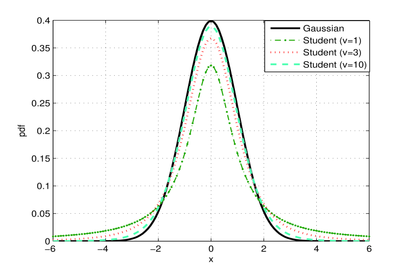
Figure 1: Comparison between the univariate Gaussian and Student’s t distributions (represented by “Student” in the figure). All distributions have zero mean with a fixed variance 1. $v$ denotes the DoF.

III-B ESTDA

In ESTDA, the probabilistic model $p(x|\theta)$ in Algorithm 1 is specified to be a student’s $t$ distribution, namely $p(x|\theta)=\mathcal{S}(x|\mu,\Sigma,v)$, where $\theta\triangleq\{\mu,\Sigma\}$, and $v$ is specified beforehand as a constant.

First, let’s figure out, given the parameter value $\theta$, how to sample an individual $x$ from $p(\cdot|\theta)$. It consists of two steps that is simulating a random draw $\tau$ from the gamma distribution, whose shape and scale parameters are set identically to $v/2$, and sampling $x$ from the Gaussian distribution $\mathcal{N}(\cdot|\mu,\Sigma/\tau)$.

Now let’s focus on, given a set of selected individuals $\{x_{j}\}_{j=1}^{M}$, how to update the parameters of the student’s $t$ distribution in a optimal manner in terms of maximizing likelihood. As mentioned above, in generation of $\{x_{j}\}_{j=1}^{M}$, a corresponding set of gamma distributed variables $\{\tau_{j}\}_{j=1}^{M}$ is used. We can record these gamma variables and then use them to easily derive an ML estimate for parameters of the Student’s $t$ distribution [23, 24]:

$$\mu = \frac{\sum_{j=1}^{M}\tau_{j}x_{j}}{\sum_{i=1}^{M}\tau_{i}}$$ (10)

$$\Sigma = \frac{\sum_{j=1}^{M}\tau_{j}(x_{j}-\mu)(x_{j}-\mu)^{T}}{\sum_{i=1}^{M}\tau_{i}}.$$ (11)

III-C EMSTDA

The EMSTDA employs a mixture of student’s $t$ distributions to play the role of the probabilistic model $p(x|\theta)$ in Algorithm 1. Now we have $p(x|\theta)=\sum_{l=1}^{L}w_{l}\mathcal{S}(x|\mu_{l},\Sigma_{l},v)$, where $\theta\triangleq\{w_{l},\mu_{l},\Sigma_{l}\}_{l=1}^{L}$, $\sum_{l=1}^{L}w_{l}=1$, and $v$ is specified beforehand as a constant. Given the selected individuals $\{x_{j}\}_{j=1}^{M}$, we resort to the EM method to update parameter values of the mixture of Student’s $t$ distributions. The specific operations are presented in Algorithm 3. EM methods based parameter estimation for the mixture of Student’s $t$ model can also be found in [14, 13, 15], where the mixture learning procedure is performed based on a weighted sample set. The EM operations presented in Algorithm 3 can be regarded as an application of the EM methods described in [14, 13, 15] to an equally weighted sample set. Similarly as in Algorithm 2, we add a components deletion operation at the end of Expectation step. This deletion operation were used in the adaptive annealed importance sampling [14] algorithm and the PE-SMC algorithm [13], which also adopt the EM procedure to do parameter estimation for a Student’s $t$ mixture model. By deleting components with extremely small mixing weights, we can avoid consuming computing burdens to update parameter values for negligible components. As presented before in Subsection II-C, this deletion operation is also useful to avoid common numerical issues such as singularity of covariance matrix. For the influence of this operation on the the number of survival mixing components, see Subsection IV-B.

Input: the individuals $\{x_{j}\}_{j=1}^{M}$, the model’s current parameter value $\theta_{k-1}=\{w_{k-1,l},\mu_{k-1,l},\Sigma_{k-1,l}\}_{l=1}^{L}$ and the admittable smallest weight $W$ of a mixing component (we set $W=0.02$ as a default value for use in our experiments)

Output: $\theta_{k}$

1 Initialization: Set $\theta_{old}=\theta_{k-1}$. Set the iteration index $i=1$;

2 while the stopping criterion is not met do

3       The Expectation step:

$$w_{new,l}=\sum_{j=1}^{M}\epsilon(l|x_{j})/M,\quad l=1,\ldots,L,$$ (12)

where $\epsilon(l|x_{j})$ denotes the probability of the event individual $x_{j}$ belonging to the $l$th mixing component, which is calculated as follows

$$\epsilon(l|x_{j})=\frac{w_{old,l}\mathcal{S}(x_{j}|\mu_{old,l},\Sigma_{old,l},v)}{\sum_{l=1}^{L}w_{old,l}\mathcal{S}(x_{j}|\mu_{old,l},\Sigma_{old,l},v)}.$$ (13)

Delete mixing components whose mixing weights are smaller than $W$. Then update the value of $L$ and increase the mixing weights of the remaining mixing components proportionally to guarantee that their summation equals 1;

4       The Maximization step:

$$\mu_{new,l} = \frac{\sum_{j=1}^{M}\epsilon(l|x_{j})x_{j}(v+d)/\left(v+M_{d}(x_{j},\mu_{old,l},\Sigma_{old,l})\right)}{\sum_{j=1}^{M}\epsilon(l|x_{j})(v+d)/\left(v+M_{d}(x_{j},\mu_{old,l},\Sigma_{old,l})\right)},\;l=1,\ldots,L,$$ (14)

$$\Sigma_{new,l} = \frac{\sum_{j=1}^{M}\epsilon(l|x_{j})(x_{j}-\mu_{new,l})(x_{j}-\mu_{new,l})^{T}(v+d)/\left(v+M_{d}(x_{j},\mu_{old,l},\Sigma_{old,l})\right)}{\sum_{j=1}^{M}\epsilon(l|x_{j})},\;l=1,\ldots,L.$$ (15)

Set $\theta_{new}=\{w_{new,l},\mu_{new,l},\Sigma_{new,l}\}_{l=1}^{L}$;

5       Set $\theta_{old}=\theta_{new}$ and let $k=k+1$.

6Set $\theta_{k}=\theta_{new}$;

Algorithm 3 EM procedure to estimate parameters of a mixture of student’s $t$ model within the EDA paradigm as presented in Algorithm 1

IV Performance evaluation

In this section, we evaluate the presented ESTDA and EMSTDA using a number of benchmark objective functions, which are designed and commonly used in literature for testing and comparing optimization algorithms. See the Appendix Section for details on the involved functions. The Gaussian-EDA and the GMM-EDA, which are described in Sections II-B and II-C, respectively, are involved for comparison purpose.

Although scaling up EDAs to large scale problems has become one of the biggest challenges of the field [25], it is not our intention here to discuss and investigate the applications of ESTDA and EMSTDA in high dimensional problems. The goal of this paper is to demonstrate the benefits resulted from the heavier tails of Student’s $t$ distribution in exploring the solution space and finding the global optimum through the EDA mechanism. Therefore we only consider cases with $d\leq 10$ here for ease of performance comparison.

IV-A Experimental study for ESTDA

As described in Subsection III-A, the degree of difference between the shapes of a Student’s $t$ and a Gaussian distribution mainly depends on the value of DoF $v$. This Subsection is dedicated to investigating the influence of $v$ on the performance of ESTDA through empirical studies.

We will test on six objective functions, including the Ackley, De Jong Function N.5, Easom, Rastrigin, Michalewicz and the Lèvy N.13 functions. We consider the 2D cases (i.e., $d$=2) here. These functions have diversing characteristics in their shapes and thus give representativeness to the results we will report. See the Appendix for mathematical definitions of these functions. We consider four ESTDAs, corresponding to different DoFs $v=5,10,50,100,500$, respectively. The sample size and selection size are fixed to be $N=1000$ and $M=200$ for all ESTDAs under consideration. A basic Gaussian-EDA is involved, acting as a benchmark algorithm for comparison. We run each algorithm 30 times independently and record the best solutions it obtained at the end of each iteration. We plot the means of the best fitness function values obtained over these 30 runs in Fig.2. It is shown that the ESTDA $(v=5)$, performs strikingly better than the other candidate algorithms for the Ackley, De Jong Function N.5 and Easom Functions. The ESTDA $(v=50)$ and ESTDA $(v=500)$ outperform the others significantly in handling the Rastrigin function; and, for the remaining Michalewicz and Lèvy N.13 functions, all the algorithms converge to the optima at a very similar rate. To summarize, the ESTDA outperforms the Gaussian-EDA markedly for four problems and performs similarly as the Gaussian-EDA for the other two problems considered here. This result demonstrate that, the heavier tails of the Student’s $t$ distribution can facilitate the process of exploring the solution space and thus constitute a beneficial factor for the EDA algorithms to find the global optimum faster.

(a) Ackley Function

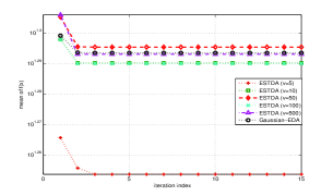
(b) De Jong Function N.5

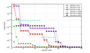
(c) Easom Function

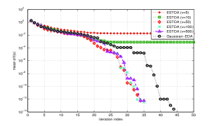
(d) Rastrigin Function

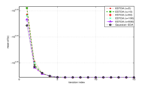
(e) Michalewicz Function

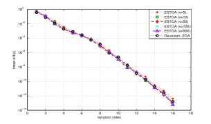
(f) Lèvy N.13 Function

Figure 2: Convergence behaviors of ESTDAs corresponding to different DoFs and a Gaussian-EDA. The Y coordinate denotes the averaged objective function values of the best solutions obtained from 30 independent runs of each algorithm. All test functions involved here are 2D

IV-B A more thorough performance evaluation for ESTDA and EMSTDA

In this subsection, we perform a more thorough performance evaluation for ESTDA and EMSTDA. Both Gassuian-EDA and GMM-EDA are also involved for comparison purpose. Including GMM-EDA we hope to further demonstrate that the heavier tails of the Student’s $t$ distribution are beneficial for exploration of solution space via the EDA mechanism. By contrasting EMSTDA with ESTDA, we can inspect how much a mixture model can contribute to search the solution space via a Student’s $t$ based EDA mechanism.

To make a representative evaluation, we will consider in total 17 objective functions listed in Table I. For all but the Rastrigin and Michalewicz functions, we consider 2D cases. For the Rastrigin and Michalewicz functions, we also consider 5D and 10D cases. The population size per iteration $N$ is set to be 1e3, 1e4, and 1e5 for 2D, 5D, 10D cases, respectively. The selection size $M$ is fixed to be $0.2\times N$ for all cases involved. We didn’t consider higher dimensional cases, for which a reliable probabilistic model building requires far more samples, while it is impractical to carry out so large numbers of samples in reasonable time scales. Definitions of all the involved objective functions are presented in the Appendix of the paper.

We fix the value of the DoF $v$ to be 5 for all test functions, except that, for problems involving the Rastrigin function, $v$ is set to be 50, since it gives better convergence behavior as reported in subsection IV-A. For every algorithm, the iterative EDA procedure terminates when the iteration number $k$ in Algorithm 1 is bigger than 50. For EMSTDA and GMM-EDA, the iterative EM procedure terminates when the iteration number $i$ in Algorithms 2 and 3 is bigger than 2. Each algorithm is run 30 times independently. Then we calculate the average and standard error of the converged fitness values. The results are given in Table I. For each test function, the best solution is marked with bold font. Then we count for each algorithm how many times it output a better solution as compared with all the rest of algorithms and put the result into Table II. We see that the EMSTDA get the highest score 7, followed by score 5 obtained by ESTDA, while their Gaussian counterparts only obtain relatively lower scores 0 and 2, respectively. This result further coincides with our argument that the Student’s $t$ distribution is more preferable than the Gaussian for use in designing EDAs. We also see that, between ESTDA and EMSTDA, the latter performs better than the former. This demonstrates that using mixture models within a Student’s $t$ based EDA is likely to be able to bring additional advantages. What slightly surprises us in Table II is that the GMM-EDA seems to perform worse than the Gaussian-EDA, while after a careful inspection on Table I, we see that GMM-EDA beats Gaussian-EDA strikingly in cases involving the Ackley, Dejong N.5, Easom, Michalewicz 10D, Eggholder, Griewank, Holder table, Schwefel and Rosenbrock functions, while for cases involving the Michalewicz 2D, Lèvy N.13, Cross-in-tray, Drop-wave, Lèvy, Schaffer, Shubert and Perm functions, GMM-EDA performs identically or similarly as the Gaussian-EDA. Hence, in summarize, GMM-EDA actually performs better than Gaussian-EDA in this experiment.

To investigate the effect of the component deletion operator used in Algorithms 3 and 2, we record the number of survival mixing components per iteration of the ESTDA and EMSTDA, and calculate its mean averaged over 30 independent runs of each algorithm. The result for six typical objective functions is depicted in Fig. 3. We see that, for both algorithms, the mean number of survival components decreases as the algorithm iterates on. This phenomenon suggests that the mixture model mainly takes effect during the early exploration stage, while, when the algorithm goes into the latter exploitation phase, there usually remains much less components in the mixture model.

TABLE I: Convergence results yielded from 30 independent runs of each algorithm on each test problem. $a\pm b$ in the table denotes that the average and standard error of the best fitness values obtained from 30 independent runs of the corresponding algorithm are $a$ and $b$, respectively. The best solution for each problem is marked with bold font.

Test Problems		Goal:$f(x^{\star})$	ESTDA	EMSTDA	Gaussian-EDA	GMM-EDA
Ackley	2D	0	0$\pm 0$	0.0128$\pm 0.0701$	3.1815$\pm 1.3004$	1.5332$\pm 1.8186$
Dejong N.5	2D	1	18.1207$\pm$1.8130	3.2370$\pm$2.6410	19.6536$\pm$1.1683	6.4677$\pm$6.3530
Easom	2D	-1	-0.9330$\pm$0.2536	-0.9587$\pm$0.1862	0.2262$\pm$0.4186	-0.3153$\pm$0.4589
Rastrigin	2D	0	0$\pm 0$	0.0050$\pm 0.0202$	0$\pm$0	0.0182$\pm 0.0643$
	5D	0	0$\pm 2.13\times 10^{-12}$	0.6562$\pm 0.7985$	0$\pm 1.70\times 10^{-11}$	0.3575$\pm 0.6293$
	10D	0	0.0383$\pm 0.0447$	0.5383$\pm 0.5980$	0.0396$\pm 0.0272$	0.5341$\pm 0.8317$
Michalewicz	2D	-1.8013	-1.8013$\pm 0$	-1.8013$\pm 0$	-1.8013$\pm 0$	-1.8013$\pm 0$
	5D	-4.6877	-4.6877$\pm 9.36\times 10^{-9}$	-4.6404$\pm 0.0561$	-4.6500$\pm 0.0099$	-4.6459$\pm 0.0175$
	10D	-9.66015	-9.5384$\pm 0.0475$	-9.4226$\pm 0.2107$	-9.1047$\pm 0.1353$	-9.1426$\pm 0.1415$
Lèvy N.13	2D	0	0$\pm 0$	0.0014$\pm 0.0053$	0$\pm$0	0.0043$\pm$0.0179
Cross-in-tray	2D	-2.0626	-2.0626$\pm$0	-2.0626$\pm$0	-2.0626$\pm$0	-2.0626$\pm$0
Drop-wave	2D	-1	-0.9884$\pm 0.0129$	-0.9909$\pm 0.0125$	-0.9990$\pm 0.0010$	-0.9938$\pm 0.0097$
Eggholder	2D	-959.6407	-588.9196$\pm$75.2446	-731.8013$\pm$145.5383	-560.7251$\pm$4.2080	-686.5236$\pm$147.5427
Griewank	2D	0	19.5764$\pm$3.7905	1.5197$\pm$5.5576	30.4232$\pm$1.0396	15.7949$\pm$16.3001
Holder table	2D	-19.2085	-19.0835$\pm$0.1918	-19.2085$\pm 0$	-19.1860$\pm$0.0821	-19.2085$\pm$0
Lèvy	2D	0	0$\pm$0	0$\pm$0	0$\pm$0	0$\pm 1.0605\times 10^{-4}$
Schaffer	2D	0	0$\pm 1.7064\times 10^{-6}$	0.0001$\pm 4.5280\times 10^{-4}$	0$\pm 0$	0$\pm 2.0208\times 10^{-4}$
Schwefel	2D	0	368.3134$\pm$75.4837	184.2835$\pm$118.4596	436.8232$\pm$2.5521	247.0598$\pm$123.2987
Shubert	2D	-186.7309	-186.7309$\pm 4.05\times 10^{-13}$	-186.7309$\pm 1.64\times 10^{-13}$	-186.7309$\pm 1.38\times 10^{-4}$	-186.7309$\pm 2.48\times 10^{-5}$
Perm	2D	0	0$\pm$0	0$\pm$0	0$\pm$0	0$\pm 4.0029\times 10^{-6}$
Rosenbrock	2D	0	0.0420$\pm 0.0418$	0.0036$\pm 0.0129$	0.0477$\pm 0.0558$	0.0151$\pm 0.0382$

TABLE II: A simple statistics made for the results presented in Table I. Each figure in this table represents the number of times the corresponding algorithm have outputted a better solution than all the rest of competitor algorithms under consideration. Note that in some cases, e.g, the Cross-in-tray function case, more than one algorithms provide an identical best solution. For such cases, no algorithm will get a score in the statistics made here.

ESTDA	EMSTDA	Gaussian-EDA	GMM-EDA
5	7	2	0

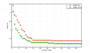
(a) Ackley Function

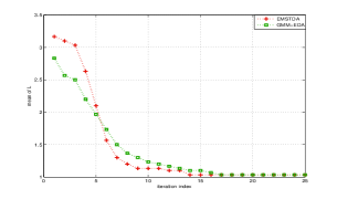
(b) De Jong Function N.5

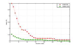
(c) Easom Function

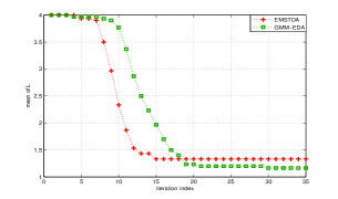
(d) Rastrigin Function

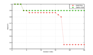
(e) Michalewicz Function

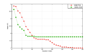
(f) Lèvy N.13 Function

Figure 3: Mean number of survival mixing components in the mixture model.

V Concluding remarks

In this paper we introduced the Student’s $t$ distribution, for the first time, into a generic paradigm of EDAs. Specifically, we developed two Student’s $t$ based EDAs, which we term as ESTDA and EMSTDA here. The justification for the proposed algorithms lies in the assumption that the heavier tails of the Student’s $t$ distribution are beneficial for an EDA type algorithm to explore the solution space. Experimental results demonstrate that for most cases under consideration, the Student’s $t$ based EDAs indeed performed remarkably better than their Gaussian counterparts implemented in the same algorithm framework. As a byproduct of our experimental study, we also demonstrated that mixture models can bring in additional advantages, for both Student’s $t$ and Gaussian based EDAs, in tackling global optimization problems.

All algorithms developed here are based on density models that use full covariance matrices. The reason is two-fold. One is for the ease of presentation of the basic idea, namely, replacing the commonly used Gaussian models by heavier tailed Student’s $t$ models in EDAs. The other is for conducting a completely fair performance comparison, since, if we combine the differing state-of-art techniques into the algorithms used for comparison, it may become difficult for us to judge whether a performance gain or loss is caused by replacing Gaussian with the Student’s $t$ model or the other state-of-art techniques. Since the full covariance model based EDA framework is so basic that many state-of-art techniques can be taken as special cases of it, we argue that the ESTDA and EMSTDA algorithms presented here can be generalized by combining other techniques, such as factorizations of the covariance matrices, dimension reduction by separating out weakly dependent dimensions or random embedding, other divide and conquer or problem decomposition approaches, to handle specific optimization problems.

APPENDIX: Benchmark objective functions used in this paper

Here we introduce the objective functions used in Section IV for testing algorithms designed to search global minimum. Note that in this section, we use $x_{i}$ to denote the $i$th dimension of $x$ for ease of exposition.

V-A Ackley Function

This function is defined to be

$$f(x)=\left[-a\exp\left(-b\sqrt{\frac{1}{d}\sum_{i=1}^{d}x_{i}^{2}}\right)-\exp\left(\frac{1}{d}\sum_{i=1}^{d}\cos(cx_{i})\right)+a+\exp(1)\right],$$ (16)

where $a=20,b=0.2$ and $c=2\pi$. This function is characterized by a nearly flat outer region, and a large peak at the centre, thus it poses a risk for optimization algorithms to be trapped in one of its many local minima. The global minima is $f(x^{\star})=0$, at $x^{\star}=(0,\ldots,0)$.

V-B De Jong Function N.5

The fifth function of De Jong is multimodal, with very sharp drops on a mainly flat surface. The function is evaluated on the square $x_{i}\in[-65.536,65.536]$, for all $i=1,2$, as follows

$$f(x)=\left(0.002+\sum_{i=1}^{2}5\frac{1}{i+(x_{1}-a_{1i})^{6}+(x_{2}-a_{2i})^{6}}\right)^{-1},$$ (17)

where

$$\mathbf{a} = \left(\begin{array}[]{ccccccccc}-32&-16&0&16&32&-32&9&16&32\\ -32&-32&-32&-32&-32&-16&32&32&32\end{array}\right).$$ (20)

The global minimum $f(x^{\star})\approx 1$ [18].

V-C Easom Function

This function has several local minimum. It is unimodal, and the global minimum has a small area relative to the search space. It is usually evaluated on the square $x_{i}\in[-100,100]$, for all i = 1, 2, as follows

$$f(x)=\cos(x_{1})\cos(x_{2})\exp\left(-(x_{1}-\pi)^{2}-(x_{2}-\pi)^{2}\right).$$ (21)

The global minimum $f(x^{\star})=-1$ is located at $x^{\star}=(\pi,\pi)$.

V-D Rastrigin Function

This function is evaluated on the hypercube $x_{i}\in[-5.12,5.12]$, for all $i=1,\ldots,d$, with the form

$$f(x)=\left(10d+\sum_{i=1}^{d}[x_{i}^{2}-10\cos(2\pi x_{i})]\right).$$ (22)

Its global minimum $f(x^{\star})=0$ is located at $x^{\star}=(0,\ldots,0)$. This function is highly multimodal, but locations of the local minima are regularly distributed.

V-E Michalewicz Function

This function has $d!$ local minima, and it is multimodal. The parameter $m$ defines the steepness of the valleys and ridges; a larger $m$ leads to a more difficult search. The recommended value of $m$ is $m=10$. It is usually evaluated on the hypercube $x_{i}\in[0,\pi]$, for all $i=1,\ldots,d$, as follows

$$f(x)=\sum_{i=1}^{d}\sin(x_{i})\sin^{2m}\left(\frac{ix_{i}^{2}}{\pi}\right).$$ (23)

The global minimum in 2D case is $f(x^{\star})=-1.8013$ located at $x^{\star}=(2.20,1.57)$, in 5D case is $f(x^{\star})=-4.687658$ and in 10D case is $f(x^{\star})=-9.66015$.

V-F Lèvy Function N.13

This function is evaluated on the hypercube $x_{i}\in[-10,10]$, for $i=1,2$, as below

$$f(x)=\left(\sin^{2}(3\pi x_{1})+(x_{1}-1)^{2}[1+\sin^{2}(3\pi x_{2})]+(x_{2}-1)^{2}[1+\sin^{2}(2\pi x_{2})]\right),$$ (24)

with global minimum $f(x^{\star})=0$, at $x^{\star}=(1,\ldots,1)$.

V-G Cross-in-tray Function

This function is defined to be

$$f(x)=\left(-0.0001\left(\left|g(x_{1},x_{2})\right|+1\right)^{0.1}\right),$$ (25)

where

$$g(x_{1},x_{2})=\sin(x_{1})\sin(x_{2})\exp\left(\left|100-\frac{\sqrt{x_{1}^{2}+x_{2}^{2}}}{\pi}\right|\right).$$

It is evaluated on the square $x_{i}\in[-10,10]$, for $i=1,2$, with $f(x^{\star})=-2.06261$. This function has multiple global minima located at $x^{\star}=$ $(1.3491,-1.3491),$ $(1.3491,1.3491),$ $(-1.3491,1.3491)$ and $(-1.3491,-1.3491)$.

V-H Drop-wave Function

This is multimodal and highly complex function. It is evaluated on the square $x_{i}\in[-5.12,5.12]$, for $i=1,2$, as follows

$$f(x)=-\frac{1+\cos(12\sqrt{x_{1}^{2}+x_{2}^{2}})}{0.5(x_{1}^{2}+x_{2}^{2})+2}.$$ (26)

The global minimum $f(x^{\star})=-1$ is located at $x^{\star}=(0,0)$.

V-I Eggholder Function

This is a difficult function to optimize, because of a large number of local minima. It is evaluated on the square $x_{i}\in[-512,512]$, for $i=1,2,$ as follows

$$f(x)=\left[-(x_{2}+47)\sin\left(\sqrt{\left|x_{2}+\frac{x_{1}}{2}+47\right|}\right)-x_{1}\sin\left(\sqrt{|x_{1}-(x_{2}+47)|}\right)\right].$$ (27)

The global minimum $f(x^{\star})=-959.6407$ is located at $x^{\star}=(512,404.2319)$.

V-J Griewank Function

This function has many widespread local minima, which are regularly distributed. It is usually evaluated on the hypercube $x_{i}\in[-600,600]$, for all $i=1,\ldots,d$, as follows

$$f(x)=\left(\sum_{i=1}^{d}\frac{x_{i}^{2}}{4000}-\prod_{i=1}^{d}\cos\left(\frac{x_{i}}{\sqrt{i}}\right)+1\right).$$ (28)

The global minimum $f(x^{\star})=0$ is located at $x^{\star}=(0,\ldots,0)$.

V-K Holder table Function

This function has many local minimum, with four global one. It is evaluated on the square $x_{i}\in[-10,10]$, for $i=1,2$, as follows

$$f(x)=-\left|\sin(x_{1})\cos(x_{2})\exp\left(\left|100-\frac{\sqrt{x_{1}^{2}+x_{2}^{2}}}{\pi}\right|\right)\right|.$$ (29)

Its global minimum $f(x^{\star})=-19.2085$ is located at $x^{\star}=(8.05502,9.66459),(8.05502,-9.66459),(-8.05502,9.66459)$ and $(-8.05502,-9.66459)$.

V-L Lèvy Function

This function is evaluated on the hypercube $x_{i}\in[-10,10]$, for all $i=1,\ldots,d$, as follows

$$f(x)=\left(\sin^{2}(\pi w_{1})+\sum_{i=1}^{d-1}(w_{i}-1)^{2}[1+10\sin^{2}(\pi w_{i}+1)]+(w_{d}-1)^{2}[1+\sin^{2}(2\pi w_{d})]\right).$$ (30)

where $w_{i}=1+\frac{x_{i}-1}{4}$, for all $i=1,\ldots,d$. The global minimum $f(x^{\star})=0$ is located at $x^{\star}=(1,\ldots,1)$.

V-M The second Schaffer Function

This function is usually evaluated on the square $x_{i}\in[-100,100]$, for all $i=1,2$. It has a form as follows

$$f(x)=\left(0.5+\frac{\sin^{2}(x_{1}^{2}-x_{2}^{2})-0.5}{[1+0.001(x_{1}^{2}+x_{2}^{2})]^{2}}\right).$$ (31)

Its global minimum $f(x^{\star})=0$ is located at $x^{\star}=(0,0)$.

V-N Schwefel Function

This function is also complex, with many local minima. It is evaluated on the hypercube $x_{i}\in[-500,500]$, for all $i=1,\ldots,d$, as follows

$$f(x)=\left(418.9829d-\sum_{i=1}^{d}x_{i}\sin(\sqrt{|x_{i}|})\right).$$ (32)

Its global minimum $f(x^{\star})=0$ is located at $x^{\star}=(420.9687,\ldots,420.9687)$.

V-O Shubert Function

This function has several local minima and many global minima. It is usually evaluated on the square $x_{i}\in[-10,10]$, for all $i=1,2$.

$$f(x)=\left(\sum_{i=1}^{5}i\cos((i+1)x_{1}+i)\right)\left(\sum_{i=1}^{5}i\cos((i+1)x_{2}+i)\right).$$ (33)

Its global minimum is $f(x^{\star})=-186.7309$.

V-P Perm Function 0,d,$\beta$

This function is evaluated on the hypercube $x_{i}\in[-d,d]$, for all $i=1,\ldots,d$, as follows

$$f(x)=\left(\sum_{i=1}^{d}\left(\sum_{j=1}^{d}(j+\beta)\left(x_{j}^{i}-\frac{1}{j^{i}}\right)\right)^{2}\right).$$ (34)

Its global minimum $f(x^{\star})=0$ is located at $x^{\star}=(1,\frac{1}{2},\ldots,\frac{1}{d})$.

V-Q Rosenbrock Function

This function is also referred to as the Valley or Banana function. The global minimum lies in a narrow, parabolic spike. However, even though this spike is easy to find, convergence to the minimum is difficult [26]. It has the following form

$$f(x)=\sum_{i=1}^{d-1}[100(x_{i+1}-x_{i}^{2})^{2}+(x_{i}-1)^{2}],$$ (35)

and is evaluated on the hypercube $x_{i}\in[-5,10]$, for all $i=1,\ldots,d$. The global minimum $f(x^{\star})=0$ is located at $x^{\star}=(1,\ldots,1)$.

References

- [1] M. Pelikan, D. E. Goldberg, and F. G. Lobo, “A survey of optimization by building and using probabilistic models,” Computational optimization and applications, vol. 21, no. 1, pp. 5–20, 2002.
- [2] M. Hauschild and M. Pelikan, “An introduction and survey of estimation of distribution algorithms,” Swarm and Evolutionary Computation, vol. 1, no. 3, pp. 111–128, 2011.
- [3] Q. Zhang and H. Muhlenbein, “On the convergence of a class of estimation of distribution algorithms,” IEEE Trans. on evolutionary computation, vol. 8, no. 2, pp. 127–136, 2004.
- [4] P. Larranaga and J. A. Lozano, Estimation of distribution algorithms: A new tool for evolutionary computation. Springer Science & Business Media, 2002, vol. 2.
- [5] M. Sebag and A. Ducoulombier, “Extending population-based incremental learning to continuous search spaces,” in International Conf. on Parallel Problem Solving from Nature. Springer, 1998, pp. 418–427.
- [6] P. Larrañaga, R. Etxeberria, J. A. Lozano, and J. M. Peña, “Optimization in continuous domains by learning and simulation of gaussian networks,” 2000.
- [7] P. A. Bosman and D. Thierens, “Expanding from discrete to continuous estimation of distribution algorithms: The IDEA,” in International Conference on Parallel Problem Solving from Nature. Springer, 2000, pp. 767–776.
- [8] W. Dong, T. Chen, P. Tiňo, and X. Yao, “Scaling up estimation of distribution algorithms for continuous optimization,” IEEE Trans. on Evolutionary Computation, vol. 17, no. 6, pp. 797–822, 2013.
- [9] Q. Zhang, J. Sun, E. Tsang, and J. Ford, “Hybrid estimation of distribution algorithm for global optimization,” Engineering computations, vol. 21, no. 1, pp. 91–107, 2004.
- [10] Q. Lu and X. Yao, “Clustering and learning gaussian distribution for continuous optimization,” IEEE Trans. on Systems, Man, and Cybernetics, Part C (Applications and Reviews), vol. 35, no. 2, pp. 195–204, 2005.
- [11] C. W. Ahn and R. S. Ramakrishna, “On the scalability of real-coded bayesian optimization algorithm,” IEEE Trans. on Evolutionary Computation, vol. 12, no. 3, pp. 307–322, 2008.
- [12] H. Wu and J. L. Shapiro, “Does overfitting affect performance in estimation of distribution algorithms,” in Proc. of the 8th annual conf. on Genetic and evolutionary computation. ACM, 2006, pp. 433–434.
- [13] B. Liu, “Posterior exploration based sequential monte carlo for global optimization,” arXiv preprint arXiv:1509.08870, 2015.
- [14] ——, “Adaptive annealed importance sampling for multimodal posterior exploration and model selection with application to extrasolar planet detection,” The Astrophysical Journal Supplement Series, vol. 213, no. 1, p. 14, 2014.
- [15] O. Cappé, R. Douc, A. Guillin, J.-M. Marin, and C. P. Robert, “Adaptive importance sampling in general mixture classes,” Statistics and Computing, vol. 18, no. 4, pp. 447–459, 2008.
- [16] K. L. Lange, R. J. Little, and J. M. Taylor, “Robust statistical modeling using the t distribution,” Journal of the American Statistical Association, vol. 84, no. 408, pp. 881–896, 1989.
- [17] B. Liu and C. Ji, “A general algorithm scheme mixing computational intelligence with bayesian simulation,” in Proc. of the 6th Int’l Conf. on Advanced Computational Intelligence (ICACI). IEEE, 2013, pp. 1–6.
- [18] X. Yao, Y. Liu, and G. Lin, “Evolutionary programming made faster,” IEEE Trans. on Evolutionary Computation, vol. 3, no. 2, pp. 82–102, 1999.
- [19] J. A. Bilmes et al., “A gentle tutorial of the EM algorithm and its application to parameter estimation for Gaussian mixture and hidden markov models,” International Computer Science Institute, vol. 4, no. 510, p. 126, 1998.
- [20] L. Xu and M. I. Jordan, “On convergence properties of the EM algorithm for Gaussian mixtures,” Neural computation, vol. 8, no. 1, pp. 129–151, 1996.
- [21] C. Biernacki, G. Celeux, and G. Govaert, “Choosing starting values for the EM algorithm for getting the highest likelihood in multivariate Gaussian mixture models,” Computational Statistics & Data Analysis, vol. 41, no. 3, pp. 561–575, 2003.
- [22] N. Vlassis and A. Likas, “A greedy EM algorithm for Gaussian mixture learning,” Neural processing letters, vol. 15, no. 1, pp. 77–87, 2002.
- [23] C. Liu, “ML estimation of the multivariatetdistribution and the EM algorithm,” Journal of Multivariate Analysis, vol. 63, no. 2, pp. 296–312, 1997.
- [24] C. Liu and D. B. Rubin, “ML estimation of the t distribution using EM and its extensions, ECM and ECME,” Statistica Sinica, pp. 19–39, 1995.
- [25] K. Ata, J. Bootkrajang, and R. J. Durrant, “Toward large-scale continuous EDA: A random matrix theory perspective,” Evolutionary computation, vol. 24, no. 2, pp. 255–291, 2015.
- [26] V. Picheny, T. Wanger, and D. Ginsbourger, “A benchmark of kriging-based infill criteria for noisy optimization,” Struct Multidiscip Optim, vol. 10, p. 1007, 2013.