A Non-parametric Approach to Constrain the Transfer Function in Reverberation Mapping

Abstract

Broad emission lines of active galactic nuclei stem from a spatially extended region (broad-line region, BLR) that is composed of discrete clouds and photoionized by the central ionizing continuum. The temporal behaviors of these emission lines are blurred echoes of the continuum variations (i.e., reverberation mapping, RM) and directly reflect the structures and kinematic information of BLRs through the so-called transfer function (also known as the velocity-delay map). Based on the previous works of Rybicki & Press and Zu et al., we develop an extended, non-parametric approach to determine the transfer function for RM data, in which the transfer function is expressed as a sum of a family of relatively displaced Gaussian response functions. Therefore, arbitrary shapes of transfer functions associated with complicated BLR geometry can be seamlessly included, enabling us to relax the presumption of a specified transfer function frequently adopted in previous studies and to let it be determined by observation data. We formulate our approach in a previously well-established framework that incorporates the statistical modeling of the continuum variations as a damped random walk process and takes into account the long-term secular variations which are irrelevant to RM signals. The Application to RM data shows the fidelity of our approach.

1. Introduction

The broad-line regions (BLRs) in active galactic nuclei (AGNs), with sizes of light days to light weeks (Kaspi et al. 2000; Bentz et al. 2013), are too compact to be spatially resolved with the existing telescopes, except in a few cases in which the BLRs are magnified by gravitational lensing (Sluse et al. 2012; Guerras et al. 2013). The reverberation mapping (RM) technique provides a powerful and unique way to probe the structures and kinematics of BLRs through analyzing the temporal variation patterns of emission lines and the ionizing continuum (Blandford & McKee 1982; Peterson 1993). Over the past four decades, RM studies have successfully measured BLR sizes for $\sim 60$ nearby Seyfert galaxies and quasars (e.g., Bentz et al. 2013; Du et al. 2015). Particularly influential is the discovery that BLR sizes closely correlate with optical luminosities of (sub-Eddington) AGNs, as expected from simple photoionization theory (e.g., Kaspi et al. 2000, 2005; Bentz et al. 2013; Du et al. 2015). This relationship, in combination with the velocity widths of broad emission lines, opens up an economic way for the virial mass estimation of supermassive black holes (e.g., Vestergaard & Peterson 2006; Ho & Kim 2015). Meanwhile, velocity-binned RM analysis for several AGNs with high-quality spectroscopic data has crudely seen signatures for diverse kinematics in BLRs, including radial inflows/outflows and non-radial, virialized Keplerian rotations (Bentz et al. 2009; Denney et al. 2010; Grier et al. 2013b; Peterson 2014; Du et al. 2016).

Despite these advances, the detailed information for structures and kinematics of BLRs remain largely unknown. The major challenges are from RM data sets reliably inferring the transfer function or velocity-delay map and from obtaining the structure and kinematic information of BLRs from this map. Traditional cross-correlation analysis (e.g., Bentz et al. 2013) or the previous method using a simple specified transfer function (e.g., Rybicki & Kleyna 1994; Zu et al. 2011, 2016) yields no more than the characterized BLR sizes.

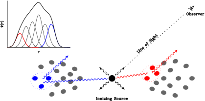
Figure 1.— Schematic of the transfer function for a system that consists of discrete clouds. The transfer function can be expressed as a sum of many relatively displaced response functions of local adjacent clouds. For illustrative purposes, the red (blue) curve in the transfer function corresponds to the response from the clouds highlighted in red (blue).

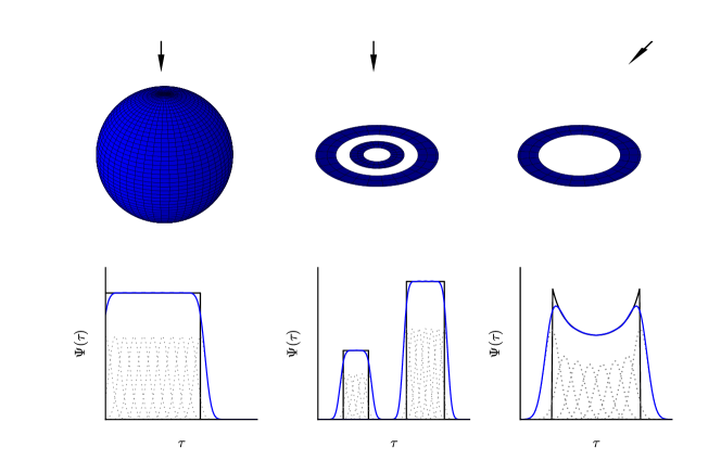
Figure 2.— Illustrative examples for three types of BLR geometry in which the transfer functions are approximated by a family of Gaussian response functions: (left) a spherical shell, (middle) two disk rings, and (right) an inclined disk ring. Arrows indicate the line of sight. In the bottom panels, black lines represent the realistic transfer functions, and blue lines represent the sum of the Gaussian functions (gray dotted lines). Our approach can particularly cope with the cases of multimodal or asymmetric transfer functions (e.g., middle panels), in which the previous JAVELIN method may encounter difficulties (see Appendix C).

Great effort has gone into developing more sophisticated methods. There are generally two classes of methods depending on the strategy adopted in solving the integral equation that links the variations of continuum and emission lines in RM. One class relies on directly inverting the integral equation, including early attempts based on the Fourier transform (Blandford & McKee 1982) and regularized linear inversion (RLI) methods (Krolik & Done 1995; Skielboe et al. 2015). The method using the Fourier transform was found to require high-fidelity data and thus has not seen much application (Maoz et al. 1991), whereas RLI seeks to discretize the integral equation and employ a differencing operator to suppress the noise. The downside of this class of methods is that the measurement noises cannot be self-consistently incorporated, thus, this class may be very noise sensitive in some cases. The other class relies on indirectly inferring the “best” transfer function that fits the data by supposing prior limits or models on it. The maximum entropy method (Horne 1994) and BLR dynamical modeling method (Pancoast et al. 2011, 2014a; Li et al. 2013) belong to this class. The maximum entropy method finds the “simplest” solutions for the transfer function by maximizing the entropy on the premise of a reasonable fit to the data. However, it does not allow for straightforward uncertainty estimates or model selection (Horne et al. 2003). The BLR dynamical modeling method presumes a specific but sufficiently flexible toy model for BLRs and directly infers the model parameters; therefore, the transfer function is only an intermediate product (Pancoast et al. 2011; Li et al. 2013). It cannot yet satisfactorily assess the systematic errors of the adopted model.

In this paper, we describe an extended, non-parametric method to determine the transfer function from RM data, based on the previous works of Rybicki & Press (1992) and Zu et al. (2011). Motivated by the scenario that BLRs are composed of a large number of clouds so that a local adjacent collection of these clouds effectively respond to the central ionizing continuum as a Gaussian response function, we express the transfer function as a sum of a family of relatively displaced Gaussian functions. Therefore, we can account for arbitrary shapes of the transfer function, thereby largely relaxing the need for presuming the transfer function (e.g., Rybicki & Kleyna 1994; Zu et al. 2011) or BLR models (e.g., Pancoast et al. 2011; Li et al. 2013). In this respect, our method is model independent and is particularly able to cope with complicated shapes of transfer functions (e.g., multimodal) for diverse BLR structures and kinematics.

The paper is organized as follows. We describe the methodology of our approach in detail in Section 2 and perform simulation tests in Section 3. Section 4 presents application of our approach to three RM AGNs to illustrate its fidelity. A discussion and conclusions are given in Section 5. All the time delays quoted in the text are given in the observer’s frame.

2. Methodology

2.1. The Transfer Function

In RM, variations of broad emission lines $f_{l}(t)$ are blurred echoes of continuum variations $f_{c}(t)$ through the transfer function $\Psi(\tau)$ as (Blandford & McKee 1982; Peterson 1993)

$$f_{l}(t)=\int_{-\infty}^{\infty}\Psi(\tau)f_{c}(t-\tau)d\tau,$$ (1)

where the integral limits are set to account for all possible positively and negatively delayed responses (e.g, Marshall et al. 2008; Shappee et al. 2014). Here, we show only velocity-unresolved RM so that velocity information is not included in the transfer function. However, it is easy to extend our approach to velocity-resolved RM by applying Equation (1) to different velocity bins of the emission lines (see below for a discussion). In addition, we also neglect the nonlinearity of the response for simplicity (Li et al. 2013). Nevertheless, we will provide below a way to incorporate non-linear response.

Mathematically speaking, it is known that an arbitrary function can be expressed as a sum of many slightly displaced $\delta-$functions—namely, $f(x)=\int f(a)\delta(x-a)da$, where $\delta(x)$ is the Dirac delta function. In practical calculations, one instead uses a set of basic functions with spatial extent to describe a smooth function. A general adoption is Gaussian functions, which are often found to be adequate (Sivia & Skilling 2006, p.140). In this spirit, the transfer function in RM is now written as

$$\Psi(\tau)=\sum_{k=1}^{K}f_{k}\exp\left[-\frac{(\tau-\tau_{k})^{2}}{2\omega^{2}}\right],$$ (2)

where $\omega$ represents the common width of Gaussian responses, $\tau_{k}$ and $f_{k}$ are the mean lag and weight of $k$th response, and $K$ is the number of responses, which can be regarded as a “smoothing parameter.” The Gaussian functions are fixed to a common width for the sake of simplicity. Such a choice also helps to relax the parameter degeneracy and improve the computational efficiency of the Bayesian inference described below.

The physical interpretation for such an expression is straightforward. The system (i.e., BLRs) under consideration is composed of a large number of clouds. Each cloud responds to the variation of the central source as a $\delta-$response function. A collection of these local adjacent clouds effectively produce a Gaussian response function with a width. This is similar to the principle of the local optimally emitting cloud model, widely applied in photon-ionization calculations (Baldwin et al. 1995). Figure 1 shows a schematic illustration of the transfer function of BLRs. In Figure 2, we show examples for three types of BLR geometry—a spherical shell, double disk rings, and an inclined disk ring—in which the transfer function is approximated by a family of Gaussian functions. In particular, there is evidence that H$\beta$ BLRs have two distinct components (e.g., Brotherton 1996; Sulentic et al. 2000; Hu et al. 2008, 2012 and references therein), which indicate that their transfer functions may be bimodal, as illustrated in the middle panels of Figure 2.

2.2. Bayesian Inference

With Equation (2), we can directly use the framework developed by Rybicki & Press (1992) and Zu et al. (2011) to infer the best transfer function. We stress that all the formulae presented in this section have been well established by Zu et al. (2011). We list them below for the sake of completeness.

Continuum variation can be well described by a damped random walk (DRW) process (e.g., Kelly et al. 2009, 2014; Zu et al. 2011; Li et al. 2013). A DRW process is a stationary process such that its covariance function at any two times $t_{i}$ and $t_{j}$ only depend on the time difference $\Delta t=t_{i}-t_{j}$, which can be simply prescribed as

$$S_{cc}(\Delta t)=\langle f_{c}(t_{i})f_{c}(t_{j})\rangle=\sigma_{\rm d}^{2}\exp\left(-\frac{|\Delta t|}{\tau_{\rm d}}\right),$$ (3)

where angle brackets represent the statistical ensemble average, $f_{c}(t)$ is the continuum driven by the DRW process, $\tau_{\rm d}$ represents the typical damping timescale, and $\sigma_{\rm d}$ represents the standard deviation of the process on a long timescale ($\gg\tau_{\rm d}$). On a short timescale, the variation amplitude of the process is $\sigma_{\rm d}\sqrt{2t/\tau_{\rm d}}$. If this is combined with Equation (1), the covariance between the line and the continuum can be written as

$$S_{lc}(\Delta t)=\langle f_{l}(t_{i})f_{c}(t_{j})\rangle=\int_{-\infty}^{\infty}\Psi(\tau)S_{cc}(\Delta t-\tau)d\tau,$$ (4)

and the covariance of the line is

$$S_{ll}(\Delta t) = \langle f_{l}(t_{i})f_{l}(t_{j})\rangle$$ (5)

$$= \int_{-\infty}^{\infty}\int_{-\infty}^{\infty}\Psi(\tau)\Psi(\tau^{\prime})S_{cc}[\Delta t-(\tau-\tau^{\prime})]d\tau d\tau^{\prime}.$$

In Appendices A and B, we present a detailed derivation for the analytical expressions of these covariances in terms of the error function.

The Bayesian posterior probability is obtained as follows (see Rybicki & Press 1992 and Zu et al. 2011 for a thorough derivation). Let $\mathbi{y}$ be a column vector comprised of the light curves of both the continuum and the line. A set of measurements in a campaign is equal to the realization of some underlying signals with measurement noises as

$$\mathbi{y}=\mathbi{s}+\mathbi{Lq}+\mathbi{n},$$ (6)

where $\mathbi{s}$ is the signal of the variations, of which the portion for the continuum is described by a DRW process, and $\mathbi{n}$ represents the measurement noises. Here the term $\mathbi{Lq}$ is usually used to model general trends linearly varying with time in the light curves (Rybicki & Press 1992), where $\mathbi{L}$ is a matrix of known coefficients and $\mathbi{q}$ is a column vector of unknown linear fitting parameters. For example, to remove separate means of the light curves with a total of $N+M$ measurements, one just configures $\mathbi{L}$ to be a $2\times(N+M)$ matrix, where $N$ and $M$ are the number of measurements for the continuum and emission line, respectively. The matrix $\mathbi{L}$ has entries of $(1,0)$ for the continuum data points and $(0,1)$ for the line data points (Rybicki & Press 1992; Zu et al. 2013). If one desires to detrend the light curves with long-term secular variations using one-order polynomials, one needs to configure $\mathbi{L}$ as a $4\times(N+M)$ matrix (see below for details). Unless stated otherwise, we remove the means of the light curves by default in the following calculations.

The signal $\mathbi{s}$ and noise $\mathbi{n}$ are assumed to be Gaussian and independent, so that their probabilities are simply written as

$$P(\mathbi{s})\propto\frac{1}{\sqrt{|\mathbi{S}|}}\exp\left(-\frac{\mathbi{s}^{T}\mathbi{S}^{-1}\mathbi{s}}{2}\right),$$ (7)

and

$$P(\mathbi{n})\propto\frac{1}{\sqrt{|\mathbi{N}|}}\exp\left(-\frac{\mathbi{n}^{T}\mathbi{N}^{-1}\mathbi{n}}{2}\right),$$ (8)

respectively, where $\mathbi{S}=\langle\mathbi{s}\mathbi{s}\rangle$ is the covariance matrix of $\mathbi{s}$ given by Equations (3)-(5) and $\mathbi{N}=\langle\mathbi{nn}\rangle$ is the covariance matrix of $\mathbi{n}$. There is no prior information for the linear fitting parameters $\mathbi{q}$, and we assign the vector a uniform prior probability. Now the probability for a realization $\mathbi{y}$ is

$$P(\mathbi{y|\sigma,\tau_{\rm d}},\boldsymbol{\theta})\propto\iiint P(\mathbi{s})P(\mathbi{n})\delta[\mathbi{y-(s+n+Lq)}]d\mathbi{s}d\mathbi{n}d\mathbi{q},$$ (9)

where $\boldsymbol{\theta}$ represents the parameter set for the transfer function in Equation (2) and the probability $P(\mathbi{q})$ is uniform, so that it is neglected in the above integral. With some mathematical implementation, it can be shown that (Zu et al. 2011)

$$P(\mathbi{y|\sigma,\tau_{\rm d}},\boldsymbol{\theta})=\frac{1}{\sqrt{|\mathbi{C}||\mathbi{L}^{T}\mathbi{C}^{-1}\mathbi{L}|}}\exp\left(-\frac{\mathbi{y}^{T}\mathbi{C}^{-1}_{\perp}\mathbi{y}}{2}\right),$$ (10)

where $\mathbi{C=S+N}$ and $\mathbi{C}^{-1}_{\perp}=\mathbi{C}^{-1}-\mathbi{C}^{-1}\mathbi{L}(\mathbi{L}^{T}\mathbi{C}^{-1}\mathbi{L})^{-1}\mathbi{L}^{T}\mathbi{C}^{-1}$. The best estimate for $\mathbi{s}$ is (Rybicki & Press 1992)

$$\mathbi{\hat{s}}=\mathbi{SC}^{-1}(\mathbi{y-L\hat{q}}),$$ (11)

and the best estimate for the linear fitting parameter is

$$\mathbi{\hat{q}}=(\mathbi{L}^{T}\mathbi{C}^{-1}\mathbi{L})^{-1}\mathbi{L}^{T}\mathbi{C}^{-1}\mathbi{y}.$$ (12)

The corresponding variance of the best estimate is, respectively,

$$\langle\Delta\mathbi{s}^{2}\rangle=\mathbi{S}-\mathbi{SC}_{\perp}^{-1}\mathbi{S},$$ (13)

and

$$\langle\Delta\mathbi{q}^{2}\rangle=(\mathbi{L}^{T}\mathbi{C}^{-1}\mathbi{L})^{-1}.$$ (14)

The best estimate for the light curves is

$$\mathbi{\hat{y}}=\mathbi{\hat{s}}+\mathbi{L\hat{q}},$$ (15)

and the corresponding variance is

$$\langle\Delta\mathbi{y}^{2}\rangle = \mathbi{S}-\mathbi{SC}^{-1}\mathbi{S}$$ (16)

$$+(\mathbi{SC}^{-1}\mathbi{L}-\mathbi{L})(\mathbi{L}^{T}\mathbi{C}^{-1}\mathbi{L})^{-1}(\mathbi{SC}^{-1}\mathbi{L}-\mathbi{L})^{T}.$$

Note that Equations (11), (12), and (15) also provide a way to estimate the value of the light curves at some specified time that may not be one of the already measured points.

According to the Bayes’s theorem, the posterior probability distribution for the free parameter set is given by

$$P(\sigma,\tau_{\rm d},\boldsymbol{\theta}|\mathbi{y})=\frac{P(\sigma,\tau_{\rm d},\boldsymbol{\theta})P(\mathbi{y}|\sigma,\tau_{\rm d},\boldsymbol{\theta})}{P(\mathbi{y})},$$ (17)

where $P(\mathbi{y})$ is the marginal likelihood that serves as a normalization factor to the posterior probability and $P(\sigma,\tau_{\rm d},\boldsymbol{\theta})$ is the prior probability for the parameters. We maximize this posterior distribution to obtain the best estimate for the free parameters using a Markov-chain Monte Carlo (MCMC) method as described in the next section.

Long-term secular variability is incidentally detected over the duration of the campaign in some RM objects (e.g., Denney et al. 2010; Li et al. 2013; Peterson et al. 2014). Such long-term trends are uncorrelated with reverberation variations and may bias the reverberation analysis (Welsh 1999). The linear fitting parameter $\mathbi{q}$ provides a natural way to remove such trends. If the long-term trends vary linearly with time ($q_{1}+q_{2}t$), the matrix $\mathbi{L}$ has the form of (Rybicki & Press 1992; Zu et al. 2011)

$$\mathbi{L}=\left[\begin{array}[]{cccc}1&t_{1}^{c}&0&0\\ \vdots&\vdots&\vdots&\vdots\\ 0&t_{N}^{c}&0&0\\ 0&0&1&t_{1}^{l}\\ \vdots&\vdots&\vdots&\vdots\\ 0&0&1&t_{M}^{l}\\ \end{array}\right],$$ (18)

where $t_{i}^{c}$ is the $i$th time of the $N$ measurement points of the continuum and $t_{i}^{l}$ is the $i$th time of the $M$ measurement points of the line. In this case, $\mathbi{q}$ is a column vector with four entries, which represent the coefficients of the linear trends for the continuum and line data. For the long-term trends with high-order polynomial variation, one can similarly write out the matrix $\mathbi{L}$ by just adding extra columns. In our calculations, when the light curves of the emission line and the driven continuum visually show different long-term trends, we switch on the detrending procedure by assuming the trends vary linearly with time (see below for application to the RM data of Mrk 817).

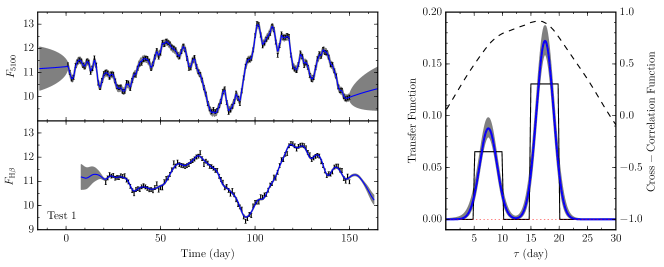
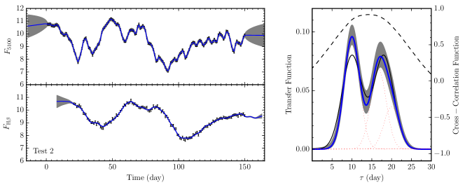
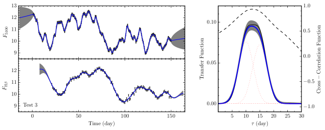
Figure 3.— Three simulation tests of our approach. Left panels: simulated light curves for 5100 Å continuum and H$\beta$ emission line. Solid lines represent the recovered light curves, and shaded areas represent their uncertainties. Right panel: the best recovered transfer function (in blue) compared with the input transfer function (in black). The shaded area represents the estimated uncertainties for the recovered transfer function. Red dotted lines represent the Gaussian functions that constitute the transfer function. Dashed lines represent the interpolation cross-correlation function of the light curves.

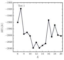
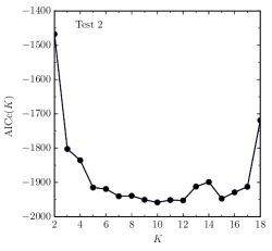
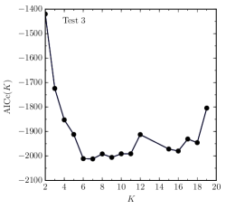
Figure 4.— The AICc as a function of the number ($K$) of Gaussian functions for the three simulation tests in Figure 3. The AICc reache a minimum at $K=13$, $10$, and $7$, respectively.

2.3. Markov-Chain Monte Carlo Implementation

The parameters in our approach include two parameters ($\sigma$ and $\tau_{d}$) pertaining to the DRW process in Equation (3) and $2K+1$ parameters ($f_{k}$s, $\tau_{k}$s, and $\omega$) pertainng to the transfer function in Equation (2). To relax parameter degeneracy, we introduce the following simplifications.

• The central lags $\tau_{k}$ of Gaussian responses are assigned by a uniformly spaced grid of time lag over a range of interests, whereas the amplitude $f_{k}$ is free to determine. Specifically, we set $\tau_{k}=\tau_{1}+(k-1)\Delta\tau$ for $1\leqslant k\leqslant K$, where $\Delta\tau$ is the grid space and $(\tau_{1},\tau_{K})$ is the range of the time lag. Given with the range of the time lag, the value of $\Delta\tau$ is determined by the number ($K$) of Gaussian functions, i.e., $\Delta\tau=(\tau_{K}-\tau_{1})/(K-1)$. The degree of freedom is now reduced to $K+3$.

• The width of Gaussian responses $\omega$ is limited by two facts. If $\omega$ is too small, unnecessary structures in transfer function will become admissible, and hence, the reconstructed light curves will appear to be unrealistically noisy; if $\omega$ is too large (e.g., $\omega>\Delta\tau$), the neighboring Gaussian responses are indeed indistinguishable. In practice, we find it is adequate to adopt a prior limit of $\omega\sim(\Delta\tau/2,\Delta\tau)$.

The prior probability $P(\sigma,\tau_{\rm d},\boldsymbol{\theta})$ in Equation (17) is assigned by assuming that all the free parameters are independent of one another. The Gaussian width has a uniform prior, and the rest of the parameters have a logarithmic prior, which is a usual choice for “scale” parameters that involve a wide range of values (e.g., Sivia & Skilling 2006, p. 108).

Lastly, we need to choose the number of Gaussian response functions. Strictly speaking, one should employ the Bayesian model selection to choose the best parameter $K$, i.e., the one that maximizes the probability $P(K|\mathbi{y})$. However, it is very computationally expensive to calculate $P(K|\mathbi{y})$ since one needs to marginalize all the other free parameters. Therefore, we resort to the relatively more economic “non-Bayesian” approaches based on the maximum-likelihood estimate of the parameters (e.g., Hooten & Hobbs 2015). We use the Akaike information criteria (AIC; Akaike 1973), measures of the relative quality of statistical models. The original form of the AIC is valid only asymptotically; Hurvich & Tsai (1989) proposed a correction to AIC for finite sample sizes (abbreviated to AICc). The AIC is defined by

$${\rm AIC}=2m-2\log P(\mathbi{y}|\hat{\sigma},\hat{\tau}_{\rm d},\boldsymbol{\hat{\theta}}),$$ (19)

where $m$ is the number of parameters in the model and the hat operator denotes the best estimate for the corresponding parameter. The AICc is defined by

$${\rm AICc}={\rm AIC}+\frac{2m(m+1)}{n-m-1},$$ (20)

where $n=N+M$ is the total number of data points. The best choice of $K$ is the one that minimizes the AICc.

We employ an MCMC method to determine the best estimates and uncertainties of free parameters. We use the Metropolis-Hastings algorithm to construct samples of free parameters from the posterior probability distribution. The Markov chain is run in 150,000 steps in total. The best estimates of free parameters are assigned the mean values of the samples, and the associated uncertainties are assigned the 68.3% confidence levels (“1$\sigma$”) that enclose the mean values. The uncertainties of the final obtained transfer function in Equation (2) are determined by the error propagation formulae, under the best inferred $K$. Therefore, the uncertainty in the best inferred $K$ is not included.

3. Simulation Tests

In order to test our approach, we generate mock light curves of the continuum and broad emission lines with an assumption of the transfer function, and then implement the above procedures to obtain the most probable estimate for the transfer function and compare it with the input one. As outlined by Rybicki & Press (1992), an unconstrained realization of mock light curves is simply a random series that has the covariance matrix $\mathbi{C=S+N}$ with specified parameters $\sigma$ and $\tau_{\rm d}$. We generate random numbers with the covariance matrix $\mathbi{C}$ using the Cholesky decomposition (see Zu et al. 2011). The Cholesky decomposition of a matrix is $\mathbi{C=MM}^{T}$, where $\mathbi{M}$ is a lower triangular matrix with real and positive diagonal entries. If $\mathbi{r}$ is a series of Gaussian random numbers with a zero mean and unity dispersion, then $\mathbi{u=Mr}$ has the covariance matrix of $\mathbi{C}$, since $\langle\mathbi{uu}^{T}\rangle=\mathbi{M}\langle\mathbi{rr}^{T}\rangle\mathbi{M}^{T}=\mathbi{MM}^{T}=\mathbi{C}$. We first generate a mock continuum light curve and then convolve it with the adopted transfer function to produce a light curve of emission line.

3.1. Validity of the Method

We run three simulation tests, presuming the transfer functions to be composed of

1. two displaced top-hats,

2. two moderately mixed Gaussians (so that the transfer function is double-peaked), and

3. two severely mixed Gaussians,

respectively. The left panels of Figure 3 plot these three input transfer functions. Specifically, for the first test, the two displaced top hats are (arbitrarily) configured to

$$\Psi(\tau)=\frac{1}{15}\times\left\{\begin{array}[]{clc}1&\rm~{}for&5<\tau<10,\\ 2&\rm~{}for&15<\tau<20,\\ 0&\rm~{}else,&\end{array}\right.$$ (21)

where 1/15 is the normalization factor. For the other two tests, the two Gaussians are (arbitrarily) configured to center at 10 and 18 days for the moderately mixed case and 10 and 15 days for the severely mixed case, with the same standard deviation of 2.5 days. The mean time lags for these three transfer functions are 14.2, 14.0, and 12.5 days, respectively, roughly corresponding to a 5100 Å luminosity of $\sim 10^{43}~{}{\rm erg~{}s^{-1}}$ according to the relation between the BLR sizes and 5100 Å luminosities of AGNs (Bentz et al. 2013). For the DRW model of all the three tests, the parameter of the damping timescale is set to $\tau_{\rm d}=80$ days, a typical value for a luminosity of $10^{43}~{}{\rm erg~{}s^{-1}}$ (Kelly et al. 2009; Zu et al. 2011; Li et al. 2013); the parameter of the variation amplitude is set to $\sigma_{\rm d}=1.5$ (in arbitrary units) such that the resulting variation amplitude is typically $\sim$30-50%. The time span of continuum monitoring is 150 days, and the monitoring of the emission line starts 20 days latter. The cadence is typically one day apart. The signal-to-noise ratio (S/N) is set to $\sim$120. It is worth stressing that the choice of these values is only for illustrative purposes and has no special meaning. The left panels of Figure 3 show the generated mock light curves of the continuum and emission lines for the three simulation tests.

Throughout the calculations, the range of the time lag is set to (0-30) days. Since the best number of Gaussians is determined by the AICc, the final transfer function is insensitive to the adopted range of time lag, provided it is broad enough to enclose the time lag of the emission line. The obtained AICc with the number of Gaussian functions $K$ for the three tests are illustrated in Figure 4. The resulting optimal $K$ are 13, 10, and 7, respectively. This means that the optimal $K$ depends not on the sampling cadence but on the shape of the transfer function. The right panels of Figure 3 show the best recovered transfer functions with the optimal $K$. As can be seen, the structures in the transfer functions are successfully recovered, and all the features in the light curves are also well reconstructed. However, we note that, in the first test, we fail to reproduce the top-hat shape because of the finite sampling and measurement errors of the light curves. Meanwhile, in the second test, although the recovered two peaks are marginally equal, the left peak seems slightly stronger than the right one. These tests suggest that, like the performance of all other RM methods, that of the present approach depends on the data quality and the presence of strong variability features in the light curves; therefore, our approach may be unable to resolve very fine structures of the transfer function in some circumstances.

On the right panels of Figure 3, we also superimpose the interpolation cross-correlation function (CCF) of the light curves using the procedure of Gaskell & Peterson (1987). All the CCFs in the three tests are single-peaked, indicating that CCF analysis hardly reveals more than the characteristic time lags of BLRs. In particular, the CCF in the first test is wide and peaks at $\tau=17.5$ day. This is an appropriate choice for the time lag if one only concentrates only on a single characteristic lag for the BLR, but clearly a single lag is not sufficient to describe the BLR in this case. In Appendix C, we show the time lag distributions from the JAVELIN method for the above three simulation tests. JAVELIN presumes a top-hat transfer function, and the time lag is assigned the mean lag of the top hat. We illustrate that while the present approach works fairly well in all the three tests, JAVELIN cannot appropriately recover the characteristic lag for the first test with a multimodal transfer function.

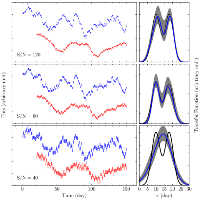
Figure 5.— Tests of our approach with S/N=120, 80, and 40. The input transfer function is presumed to be two moderately mixed Gaussians (see 3.1 for the details). For each test, the left panel shows the simulated light curves of the 5100Å continuum (in blue) and H$\beta$ line (in red), and the right panel compares the best recovered transfer function (in blue) with the input one (in black) transfer function. The shaded areas represents the estimated uncertainties for the recovered transfer function.

Figure 6.— Same as Figure 5 but for different cadences. On the top panel, the cadence is 1 day apart. On the middle and bottom panels, we randomly remove about 1/3, and 2/3, respectively, of the points.

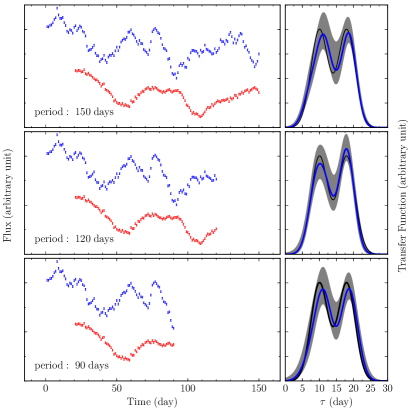
Figure 7.— Same as Figure 5 but for monitoring periods of 150, 120, and 90 days.

3.2. Dependence on Data Quality

The above simulations show that our approach can generally well reproduce the input transfer function with optimal data quality. In this section, we test the dependence of the obtained transfer function on data quality with different S/N, sampling cadences, and time spans of the mock light curves. We use for illustration only the double-peaked transfer function—namely, the one used for the second simulation test in the preceding section. We fix the seed for the random number generator so that all the mock light curves in this section have the same variation pattern. This allows us to focus only on the desired factor that influences the obtained transfer function.

In Figure 5, we generate three sets of mock light curves with S/N=120, 80, and 40, respectively. As expected, when S/N is low enough, the weak variability signals in the light curves are overwhelmed by noises, and the information of small structures in the transfer function is missing. Consequently, for the case of S/N=40 (bottom panels of Figure 5), we obtain only a single-peaked transfer function, which has the same mean time lag as the input one.

To check how the sampling rate affects the results, we respectively randomly remove about one-third and two-thirds of the points of the light curves with S/N=120 in Figure 5 and generate two new mock data sets with degraded sampling rates. We show the light curves and the corresponding best recovered transfer function in Figure 6. Again, when the sampling cadence is poorer, more information on the fine structure of the transfer function is lost.

The default time span of the light curves is 150 days. In Figure 7, we reduce the time span to 120 and 90 days, by subtracting the last 30 and 60 days section, of the light curves with S/N=120 in Figure 5, respectively. The mean time lag of the input transfer function is 14 days, so that the overall time spans are still more than six times the mean lag (Welsh 1999). There is no surprise that the transfer function is well reproduced in all the three cases in Figure 7.

In summary, provided the time span is more than several times the mean time lag of the emission line, the S/N and sampling cadence are more critical to recovering the transfer function. We stress again that the overall performance of the present approach depends on the presence of strong variation features in the light curves and the specific structures of the transfer function one desires to resolve. We therefore cannot specify more details about the data requirements for the present approach to faithfully recover the transfer function.

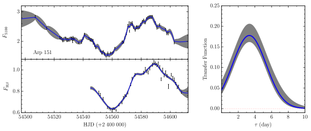
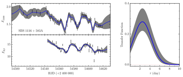
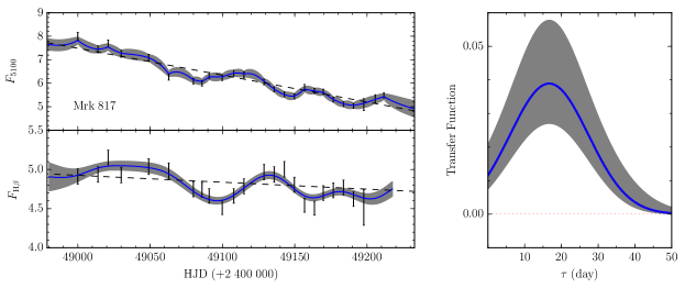
Figure 8.— The best recovered transfer functions for Arp 151 (top), SBS 1116+583A (middle), and Mrk 817 (bottom). For each object, the two left panels show the light curves of continuum and H$\beta$ line (points with error bars), together with the best reconstructions (solid lines with shaded areas). The right panel shows the best recovered transfer function, with the shaded area representing the uncertainties. Red dotted lines represent the Gaussian functions that constitute the transfer function. For Mrk 817, a detrending of the long-term trend is included. The dashed lines in the two left panels show the best fit for the detrending.

4. Application

We select three illustrative RM sources to show the feasibility of our approach: Arp 151, SBS 1116+583A, and Mrk 817. The first two objects were monitored by the Lick AGN Monitoring Project (LAMP ; Bentz et al. 2009; Walsh et al. 2009), and the last object was monitored by Peterson et al. (1998). The RM data of Arp 151 were previously studied in great detail using the maximum entropy method (Bentz et al. 2010), BLR dynamical modeling method (Brewer et al. 2011; Pancoast et al. 2014b), and RLI method (Skielboe et al. 2015). Arp 151 therefore serves as a good example to further verify the validity of our approach. The transfer function of SBS 1116+583A derived by the RLI method of Skielboe et al. interestingly showed a bimodal distribution, meriting an analysis using our approach. The object Mrk 817 shows long-term secular trends in its light curves (Li et al. 2013) and is therefore adopted to illustrate the capability of our approach for coping with detrending.

To compare our results with those of CCF analysis, we define the mean time delay from the transfer function as (Rybicki & Kleyna 1994)

$$\tau_{\rm m}=\frac{\int_{-\infty}^{\infty}\tau\Psi(\tau)d\tau}{\int_{-\infty}^{\infty}\Psi(\tau)d\tau}=\frac{\sum_{k}f_{k}\tau_{k}}{\sum_{k}f_{k}}.$$ (22)

The uncertainty of $\tau_{\rm m}$ is calculated by the error propagation formulae.

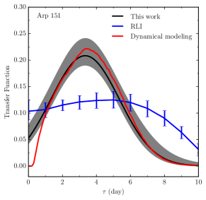
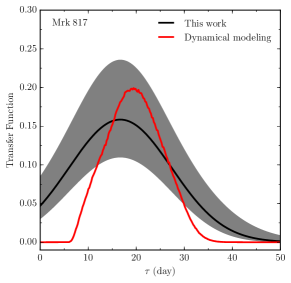
Figure 9.— Comparisons of the transfer functions derived from different methods for Arp 151 (top), SBS 1116+583A (middle), and Mrk 817 (bottom). The black line with shaded areas is the transfer function from this work, the blue line with error bars is from the regularized linear inversion (RLI) method of Skielboe et al. (2015), and the red line is from the BLR dynamical modeling method of Li et al. (2013). Note that there is no RLI solution for Mrk 817. All the transfer functions are normalized on a common scale.

4.1. Arp 151

For the sake of comparison with the previous results, we use the $B-$band photometric light curve of Arp 151 as a surrogate of the continuum as in Pancoast et al. (2014b) and Skielboe et al. (2015). The magnitudes are first converted into fluxes. Since the absolute unit of light curves is no longer important for RM analysis, we adopt an arbitrary zero-magnitude flux for the conversion. We set the range of the time lag for solving the transfer function to be (0-10) days. The best number of Gaussian functions is $K=4$ according the AICc.

The top panels of Figure 8 present the reconstruction for the light curves of the continuum and H$\beta$ line and the best recovered transfer function for Arp 151. The mean time lag from Equation (22) is $\tau_{\rm m}=3.33\pm 0.26$ days, consistent with the previous results from CCF analysis, $\tau_{\rm CCF}=4.08\pm 0.60$ days (Bentz et al. 2009), and the JAVELIN method of Zu et al. (2011), $\tau_{\rm JAV}=3.68\pm 0.36$ days (Grier et al. 2013a). The transfer function is mainly contributed by the second Gaussian component centered at $\tau=3.33$ days.

On the top panel of Figure 9, we compare the transfer function derived in this work with those derived from the RLI method (Skielboe et al. 2015) and from the BLR dynamical method (Li et al. 2013). Our result well matches that from the dynamical modeling method but differs from the RLI result, which has a plateau from 0 to about 7 days. The shape of our obtained transfer function also coincides with that from the maximum entropy method (see Figure 1 in Bentz et al. 2010).

4.2. SBS 1116+583A

As we have done for for Arp 151, we use the $B-$band photometric light curve for this object. The range of the time lag in the calculations is set to (0-10) days, and the best number of Gaussian functions is $K=5$ according to the AICc. The results are shown on the middle panels of Figure 8. The obtained mean time lag is $\tau_{\rm m}=2.50\pm 0.70$ days, which is again well consistent with the results based on CCF analysis, $\tau_{\rm CCF}=2.38\pm 0.58$ days (Bentz et al. 2009), and the JAVELIN method, $\tau_{\rm JAV}=2.46\pm 0.93$ days (Grier et al. 2013a).

The middle panel of Figure 9 compares the derived transfer functions from various methods. The RLI method yields a bimodal transfer function with a response component of around 2 days and an additional component of around 8 days (Skielboe et al. 2015). However, both the transfer functions obtained in this work and those from the dynamical modeling do not show the second component. An inspection of the reconstructed H$\beta$ light curves (see Figure 10 in Skielboe et al. 2015) indicates that our results better match the observations.

4.3. Mrk 817

Mrk 817 was monitored for as long as five years by Peterson et al. (1998), but only during the intervening three years were H$\beta$ time lags detected. We use the first-year section of the light curves with the H$\beta$ time lags detected (HJD 24,449,000$-$24,449,211). The CCF analysis by Peterson et al. (1998) yielded a time lag of $\tau_{\rm CCF}=20.1\pm 4.4$ days. The range of the time lag in our calculations is set to (0-50) days and the best number of Gaussian functions is found to be $K=4$. It is apparent from a simple visual inspection that the light curves of the continuum and H$\beta$ line show different long-term trends, with that of the continuum fluxes decreasing more steeply. We therefore include the detrending procedure as described in Section 2.2, in which both the trends of both the continuum and the H$\beta$ line are modeled by a linear polynomial. The results are plotted on the bottom panels of Figure 8. The transfer function peaks at around 17 days and bears large uncertainties due to poor data sampling. The resulting mean time lag also has a fairly large uncertainty $\tau_{\rm m}=16.7\pm 8.3$ days. Nevertheless, all the variation features in the light curves are well reproduced.

This object has never been analyzed by the RLI method or the maximum entropy method. The bottom panel of Figure 9 only shows a comparison of our result with only that of the dynamical modeling method. The two results are generally consistent, although our result peaks at a slightly shorter time lag.

In our application to the above three RM objects, the transfer functions can be effectively modeled by a single Gaussian. As illustrated in Section 3.2, the time resolution of the obtained transfer function is determined by the data sampling and measurement noises of the observations. In a statistical sense, based on the AICc criteria, the present solutions are the best ones that balance the trade-off between the goodness of fit and the complexity of our approach. Refining the sampling and signal-to-noise ratio can certainly provide more constraints on the fine structures in transfer functions (see Figure 2) if they are not intrinsically a simple single Gaussian.

5. Discussion and Conclusions

By extending the previous work of Rybicki & Press (1992) and Zu et al. (2011), we describe a non-parametric approach to determine the transfer function in RM. The basic principle that the transfer function can be expressed as a sum of a family of relatively displaced Gaussian functions enables us to largely obviate the need for the presumption of a specified transfer function or BLR model as in previous studies. Thus, this to some extent makes our approach model independent. In addition, following the framework of Zu et al. (2011), the inclusion of the statistical modeling of continuum variations as a DRW process allows us to naturally take into account the measurement errors and make use of the information in observation data sets as much as possible. The application of our approach to RM data sets illustrates its fidelity of our approach and its capability to deal with long-term, secular variations in light curves. In particular, our approach is apt for solving the multimodal transfer functions associated with multiple-component structures of BLRs (e.g., Hu et al. 2012). In addiation to BLRs, our approach can also be applied to RM observations of dusty tori in AGNs (e.g., Suganuma et al. 2006; Koshida et al. 2014).

Since we relax the presumption of a specified transfer function but let its shape be determined by the data, our approach can be regarded as a useful complementary to the BLR dynamical modeling (Pancoast et al. 2011, 2014a; Li et al. 2013). Indeed, interpretation of the obtained transfer functions has to invoke physical BLR models. A combination of these two methods may help to remove the concern over the systematic errors in the dynamical modeling. On the other hand, in our approach (compared with the RLI method and the maximum entropy method), we incorporate the statistical description for the light curves of both the continuum and the emission line; therefore, we take full advantage of the information in the data and can estimate uncertainties for the obtained transfer function in a self-consistent manner.

We end with discussions on some potential improvements to be made to our approach.

• Throughout our calculations, we have by default assumed a linear response of the emission line to the continuum so that the covariance functions of the light curves can be analytically expressed by the error function. To include nonlinear response (Li et al. 2013), we can introduce a new parameter $\gamma$ for the emission line fluxes as

  $$f_{l}(t)=f_{l,\rm new}^{1+\gamma}(t),$$ (23)

  so that the new flux series $f_{l,\rm new}(t)$ now linearly responds to the continuum.

• Since our approach is based on the statistical modeling of the temporal variations, it is not straightforward to directly include the velocity information. We can apply our approach to each velocity bin individually (e.g., Skielboe et al. 2015). In this case, any correlation information between velocity bins is neglected; thus, the obtained velocity-resolved transfer function may be noisy along the velocity direction. It merits a future development of a feasible scheme to self-consistently take into account the velocity information.

• We use the DRW process to describe the continuum variations, a process found to be sufficiently adequate for most of current AGN variability data sets (e.g., Kelly et al. 2009; MacLeod et al. 2010; Li et al. 2013; Zu et al. 2013). However, there is evidence that the DRW process is no longer appropriate on a short time scale of days (Mushotzky et al. 2011; Kasliwal et al. 2015; Kozlowski 2016). This impedes the application of our approach in recovering very fine structures (on a timescale of days) in the transfer function. Recently, Kelly et al. (2014) developed a flexible method that statistically describes the variability by a general continuous-time autoregressive moving average (CARMA) process. The DRW process is a special case of the CARMA process. In principle, our approach can also naturally include the CARMA process, but this will make out approach highly computationally expensive. We therefore defer this to a future improvement with the parallelization of our approach on supercomputer clusters.

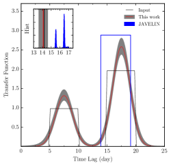
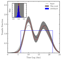
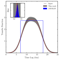
Figure 10.— Comparison of the best recovered transfer functions from our approach (red lines with shaded areas) with JAVELIN (blue lines) for the simulated light curves of the three tests in Figure 3. Black lines show the input transfer functions. The transfer functions are adjusted to a common scale. The inset panels highlight the histograms of the mean time lags of the top hat from JAVELIN, along with the mean time lags of the transfer functions from the input and our approach, indicated by black vertical lines and red vertical lines with shaded areas, respectively.

Appendix A
Covariance functions

In this appendix, we derive analytical expressions for $S_{lc}$ and $S_{ll}$ in Equations (4) and (5). In deriving $S_{lc}$, for the sake of clarity, we denote

$$S_{lc}(\Delta t)=\sum_{k}S_{lc}^{k}(\Delta t),$$ (24)

where $S_{lc}^{k}$ represents the contribution to the covariance from the $k$th Gaussian component. It is easy to show

$$S_{lc}^{k}(\Delta t) = \sigma^{2}f_{k}\left[\int_{-\infty}^{\Delta t}+\int_{\Delta t}^{\infty}\right]e^{-(\tau-\tau_{k})^{2}/2\omega^{2}-|\tau-\Delta t|/\tau_{d}}d\tau$$ (25)

$$= \sqrt{\frac{\pi}{2}}\sigma^{2}\omega f_{k}e^{\omega^{2}/2\tau_{\rm d}^{2}}\left\{e^{-\Delta T_{1}/\tau_{\rm d}}{\rm erfc}\left[-\frac{1}{\sqrt{2}}\left(\frac{\Delta T_{1}}{\omega}-\frac{\omega}{\tau_{\rm d}}\right)\right]\right.$$

$$\left.+e^{\Delta T_{1}/\tau_{\rm d}}{\rm erfc}\left[\frac{1}{\sqrt{2}}\left(\frac{\Delta T_{1}}{\omega}+\frac{\omega}{\tau_{\rm d}}\right)\right]\right\},$$

where $\Delta T_{1}=\Delta t-\tau_{k}$ and ${\rm erfc}(x)$ is the complementary error function.

Similarly, we denote

$$S_{ll}(\Delta t)=\sum_{k}\sum_{m}S_{ll}^{km}(\Delta t).$$ (26)

The covariance component $S_{ll}^{km}$ is

$$S_{ll}^{km}(\Delta t) = \sigma^{2}f_{k}f_{m}\int_{-\infty}^{\infty}\int_{-\infty}^{\infty}e^{-(\tau-\tau_{k})^{2}/2\omega^{2}}e^{-(\tau^{\prime}-\tau_{m})^{2}/2\omega^{2}}$$ (27)

$$\times e^{-|\Delta t-(\tau-\tau^{\prime})|/\tau_{\rm d}}d\tau^{\prime}d\tau.$$

Introducing new variables $u=(\tau+\tau^{\prime})$ and $v=(\tau-\tau^{\prime})$, we have

$$S_{ll}^{km}(\Delta t) = \frac{1}{2}f_{m}f_{k}\sigma^{2}\int_{-\infty}^{\infty}du\int_{-\infty}^{\infty}dve^{-(u+v-2\tau_{k})^{2}/8\omega^{2}}$$ (28)

$$\times e^{-(u-v-2\tau_{m})^{2}/8\omega^{2}}e^{-|\Delta t-v|/\tau_{\rm d}}.$$

Note that

$$(u+v-2\tau_{k})^{2}+(u-v-2\tau_{m})^{2}$$

$$=2\left[u-(\tau_{k}+\tau_{m})\right]^{2}+2\left[v-(\tau_{k}-\tau_{m})\right]^{2}.$$ (29)

The above integral can be rewritten as

$$S_{ll}^{km}(\Delta t) = \frac{1}{2}f_{m}f_{k}\sigma^{2}\int_{-\infty}^{\infty}due^{-[u-(\tau_{k}+\tau_{m})]^{2}/4\omega^{2}}$$ (30)

$$\times\int_{-\infty}^{\infty}dve^{-[v-(\tau_{k}-\tau_{m})]^{2}/4\omega^{2}-|\Delta t-v|/\tau_{\rm d}}.$$

The first integration term is

$$\int_{-\infty}^{\infty}e^{-[u-(\tau_{k}+\tau_{m})]^{2}/4\omega^{2}}du=2\sqrt{\pi}\omega,$$ (31)

and the second integration term is

$$\left[\int_{-\infty}^{\Delta t}\right. + \left.\int^{\infty}_{\Delta t}\right]e^{-[v-(\tau_{k}-\tau_{m})]^{2}/4\omega^{2}-|\Delta t-v|/\tau_{\rm d}}dv$$ (32)

$$= \sqrt{\pi}\omega e^{\omega^{2}/\tau_{\rm d}^{2}}\left\{e^{-\Delta T_{2}/\tau_{\rm d}}{\rm erfc}\left[-\frac{\Delta T_{2}}{2\omega}+\frac{\omega}{\tau_{\rm d}}\right]\right.$$

$$\left.+e^{\Delta T_{2}/\tau_{\rm d}}{\rm erfc}\left[\frac{\Delta T_{2}}{2\omega}+\frac{\omega}{\tau_{\rm d}}\right]\right\},$$

where $\Delta T_{2}=\Delta t-(\tau_{k}-\tau_{m})$. As a result, we arrive at

$$S_{ll}^{km}(\Delta t) = \pi\omega^{2}f_{m}f_{k}\sigma^{2}e^{\omega^{2}/\tau_{\rm d}^{2}}\left\{e^{-\Delta T_{2}/\tau_{\rm d}}{\rm erfc}\left[-\frac{\Delta T_{2}}{2\omega}+\frac{\omega}{\tau_{\rm d}}\right]\right.$$ (33)

$$\left.+e^{\Delta T_{2}/\tau_{\rm d}}{\rm erfc}\left[\frac{\Delta T_{2}}{2\omega}+\frac{\omega}{\tau_{\rm d}}\right]\right\}.$$

Appendix B
Error function

The error function is defined as

$${\rm erf}(x)=\frac{2}{\sqrt{\pi}}\int^{x}_{0}e^{-t^{2}}dt.$$ (34)

The complementary error function is defined as

$${\rm erfc}(x)=1-{\rm erf}(x)=\frac{2}{\sqrt{\pi}}\int_{x}^{\infty}e^{-t^{2}}dt.$$ (35)

It is trivial to show that the integral

$$\int^{x}_{-\infty}e^{-t^{2}}dt=\frac{\sqrt{\pi}}{2}{\rm erfc}(-x),$$ (36)

and the intergal

$$\int e^{-(at^{2}+bt+c)}dt = -\frac{1}{2}\sqrt{\frac{\pi}{a}}e^{(b^{2}-4ac)/4a}$$ (37)

$$\times{\rm erfc}\left(\sqrt{a}x+\frac{b}{2\sqrt{a}}\right)+{\rm const.}$$

Appendix C
Comparison with JAVELIN

The present approach extends the work of Zu et al. (2011) by adopting a more flexible transfer function rather than a specified top-hat transfer function. Therefore, we can obtain more than the characteristic time lag and recover complicated structures in the transfer function. In Figure 10, we run the public package JAVELIN, developed by Zu et al. (2011), on the simulated light curves of the three tests in Section 3.1 and plot the obtained top-hat transfer functions and the distributions of the mean time lag of the top-hat. The recovered transfer functions from our approach and the input transfer functions are also superimposed for comparison. JAVELIN also employs an MCMC method (but with a different algorithm) to determine the best values of the free parameters. Again, we run the Markov chain with 150,000 steps. The time-lag distribution for the first test is bimodal, with the two peaks at 15.53$\pm$0.04 and 16.5$\pm$0.1 days, respectively, and the overall mean lag of 16.2$\pm$0.5 days. Here, the uncertainties are assigned the standard deviations of the distributions. The two peaks correspond to neither the mean lags of the input two top hats (7.5 and 17.5 days) nor the overall mean lag (14.2 days). The JAVELIN time lags for the second and third tests are 14.0$\pm$0.2 and 12.5$\pm$0.1 days, respectively, in agreement with the mean lags of the input transfer functions (14.0 and 12.5 days). However, for the second test, the time lag does not show the expected double-peak distribution. By contrast, the present approach works fairly well in all these three cases (see Figure 3), in terms of recovering both the shape of the transfer functions and the characteristic time lags. The present approach yields a mean time lag of 14.1$\pm$0.5, 14.1$\pm$0.9, and 12.4$\pm$0.5 days for the three tests, respectively, generally consistent with the input values. Here, the uncertainties are calculated by applying the error propagation formulae to Equation (22). We attribute such discrepancies of JAVELIN to the too simplified top-hat transfer function adopted in the approach, which may encounter difficulties when the transfer function is multimodal and asymmetric.

References

- Akaike (1973) Akaike, H. 1973, in Proceedings of the Second International Symposium on Information Theory, ed. B. Petrov & F. Csaki (Budapest: Akademiai Kiado), 267
- Baldwin et al. (1995) Baldwin, J., Ferland, G., Korista, K., & Verner, D. 1995, ApJ, 455, L119
- Bentz et al. (2013) Bentz, M. C., Denney, K. D., Grier, C. J., et al. 2013, ApJ, 767, 149
- Bentz et al. (2010) Bentz, M. C., Horne, K., Barth, A. J., et al. 2010, ApJ, 720, L46
- Bentz et al. (2009) Bentz, M. C., Walsh, J. L., Barth, A. J., et al. 2009, ApJ, 705, 199
- Blandford & McKee (1982) Blandford, R. D., & McKee, C. F. 1982, ApJ, 255, 419
- Brewer et al. (2011) Brewer, B. J., Treu, T., Pancoast, A., et al. 2011, ApJ, 733, L33
- Brotherton (1996) Brotherton, M. S. 1996, ApJS, 102, 1
- Denney et al. (2010) Denney, K. D., Peterson, B. M., Pogge, R. W., et al. 2010, ApJ, 721, 715
- Du et al. (2015) Du, P., Hu, C., Lu, K.-X., et al. 2015, ApJ, 806, 22
- Du et al. (2016) Du, P., Lu, K.-X., Hu, C., et al. 2016, ApJ, 820, 27
- Gaskell & Peterson (1987) Gaskell, C. M., & Peterson, B. M. 1987, ApJS, 65, 1
- Grier et al. (2013a) Grier, C. J., Martini, P., Watson, L. C., et al. 2013a, ApJ, 773, 90
- Grier et al. (2013b) Grier, C. J., Peterson, B. M., Horne, K., et al. 2013b, ApJ, 764, 47
- Guerras et al. (2013) Guerras, E., Mediavilla, E., Jimenez-Vicente, J., et al. 2013, ApJ, 764, 160
- Ho & Kim (2015) Ho, L. C., & Kim, M. 2015, ApJ, 809, 123
- Hooten & Hobbs (2015) Hooten, M. B. and Hobbs, N. T. 2015, Ecological Monographs, 85, 3
- Horne (1994) Horne, K. 1994, in ASP Conf. Ser. 69, Reverberation Mapping of the Broad Line Region in Active Galactic Nuclei, ed. P. M. Gondhalekar, K. Horne, & B. M. Peterson (San Francisco, CA: ASP), 23
- Horne et al. (2003) Horne, K., Korista, K. T., & Goad, M. R. 2003, MNRAS, 339, 367
- Hu et al. (2008) Hu, C., Wang, J.-M., Ho, L. C., et al. 2008, ApJ, 683, L115
- Hu et al. (2012) Hu, C., Wang, J.-M., Ho, L. C., et al. 2012, ApJ, 760, 126
- Hurvich & Tsai (1989) Hurvich, C. M. & Tsai, C.-L. 1989, Biometrika, 76, 297
- Kasliwal et al. (2015) Kasliwal, V. P., Vogeley, M. S., & Richards, G. T. 2015, MNRAS, 451, 4328
- Kaspi et al. (2005) Kaspi, S., Maoz, D., Netzer, H., et al. 2005, ApJ, 629, 61
- Kaspi et al. (2000) Kaspi, S., Smith, P. S., Netzer, H., et al. 2000, ApJ, 533, 631
- Kelly et al. (2009) Kelly, B. C., Bechtold, J., & Siemiginowska, A. 2009, ApJ, 698, 895
- Kelly et al. (2014) Kelly, B. C., Becker, A. C., Sobolewska, M., Siemiginowska, A., & Uttley, P. 2014, ApJ, 788, 33
- Koshida et al. (2014) Koshida, S., Minezaki, T., Yoshii, Y., et al. 2014, ApJ, 788, 159
- Kozlowski (2016) Kozlowski, S. 2016, MNRAS, 457, 2787
- Krolik & Done (1995) Krolik, J. H., & Done, C. 1995, ApJ, 440, 166
- Li et al. (2013) Li, Y.-R., Wang, J.-M., Ho, L. C., Du, P., & Bai, J.-M. 2013, ApJ, 779, 110
- MacLeod et al. (2010) MacLeod, C. L., Ivezić, Ž., Kochanek, C. S., et al. 2010, ApJ, 721, 1014
- Marshall et al. (2008) Marshall, K., Ryle, W. T., & Miller, H. R. 2008, ApJ, 677, 880-883
- Maoz et al. (1991) Maoz, D., Netzer, H., Mazeh, T., et al. 1991, ApJ, 367, 493
- Mushotzky et al. (2011) Mushotzky, R. F., Edelson, R., Baumgartner, W., & Gandhi, P. 2011, ApJ, 743, L12
- Pancoast et al. (2011) Pancoast, A., Brewer, B. J., & Treu, T. 2011, ApJ, 730, 139
- Pancoast et al. (2014a) Pancoast, A., Brewer, B. J., & Treu, T. 2014a, MNRAS, 445, 3055
- Pancoast et al. (2014b) Pancoast, A., Brewer, B. J., Treu, T., et al. 2014b, MNRAS, 445, 3073
- Peterson (1993) Peterson, B. M. 1993, PASP, 105, 247
- Peterson (2014) Peterson, B. M. 2014, Space Sci. Rev., 183, 253
- Peterson et al. (2014) Peterson, B. M., Grier, C. J., Horne, K., et al. 2014, ApJ, 795, 149
- Peterson et al. (1998) Peterson, B. M., Wanders, I., Bertram, R., et al. 1998, ApJ, 501, 82
- Rybicki & Kleyna (1994) Rybicki, G. B., & Kleyna, J. T. 1994, in ASP Conf. Ser. 69, Reverberation Mapping of the Broad-Line Region in Active Galactic Nuclei, ed. P. M. Gondhalekar, K. Horne, & B. M. Peterson (San Francisco, CA: ASP), 85
- Rybicki & Press (1992) Rybicki, G. B., & Press, W. H. 1992, ApJ, 398, 169
- Shappee et al. (2014) Shappee, B. J., Prieto, J. L., Grupe, D., et al. 2014, ApJ, 788, 48
- Sivia & Skilling (2006) Sivia, D. S. & Skilling, J. 2006, Data Analysis: A Bayesian Tutorial (New York: Oxford Univ. Press)
- Skielboe et al. (2015) Skielboe, A., Pancoast, A., Treu, T., et al. 2015, MNRAS, 454, 144
- Sluse et al. (2012) Sluse, D., Hutsemékers, D., Courbin, F., Meylan, G., & Wambsganss, J. 2012, A&A, 544, A62
- Suganuma et al. (2006) Suganuma, M., Yoshii, Y., Kobayashi, Y., et al. 2006, ApJ, 639, 46
- Sulentic et al. (2000) Sulentic, J. W., Marziani, P., Zwitter, T., Dultzin-Hacyan, D., & Calvani, M. 2000, ApJ, 545, L15
- Vestergaard & Peterson (2006) Vestergaard, M., & Peterson, B. M. 2006, ApJ, 641, 689
- Walsh et al. (2009) Walsh, J. L., Minezaki, T., Bentz, M. C., et al. 2009, ApJS, 185, 156
- Welsh (1999) Welsh, W. F. 1999, PASP, 111, 1347
- Zu et al. (2016) Zu, Y., Kochanek, C. S., Kozłowski, S., & Peterson, B. M. 2016, ApJ, 819, 122
- Zu et al. (2013) Zu, Y., Kochanek, C. S., Kozłowski, S., & Udalski, A. 2013, ApJ, 765, 106
- Zu et al. (2011) Zu, Y., Kochanek, C. S., & Peterson, B. M. 2011, ApJ, 735, 80