Boundary control of cascaded ODE-Heat equations under actuator saturation

Abstract

In this paper, we consider boundary stabilization for a cascade of ODE-heat system with a time-varying state delay under actuator saturation. To stabilize the system, we design a state feedback controller via the backstepping method and find a bound on the domain of attraction. The latter bound is based on Lyapunov method, whereas the exponential stability conditions for the delayed cascaded system are derived by using Halanay’s inequality. Numerical examples illustrate the efficiency of the method.

1 Introduction

In the last few years, coupled systems have attracted considerable attention in research communities. Stabilization of the cascade of PDE systems was dealt with in [17, 23]. Controller design for PDE-ODE cascade systems has been extensively studied for many types of coupling such as ODE-Reaction diffusion equation (see e.g. [15, 20, 21]), ODE-Wave equation (see e.g. [16]), and ODE-Schrödinger equation (see e.g. [19]). In order to stabilize the cascaded PDE-ODE systems, the backstepping method has been applied in [19, 15, 16, 20, 21]. The idea is to use a Volterra integral transformation to transform the original system to a target system [14].

Stabilization for systems described by PDEs subject to time delay has received much attention in recent years. An effective linear matrix inequality (LMI) approach is proposed to analysis and design for time delay PDE systems in [4, 5, 6, 7, 9]. In [12], based on the backstepping method, a control strategy for reaction-diffusion equations with a constant state delay is proposed.

For practical application of backstepping controllers, in many cases the constraints on the control input should be taken into account. There have been some important results about PDEs subject to distributed control constraints (see e.g. [3, 13, 18]). However, boundary control of PDEs in the presence of actuator saturation has not been studied yet in the literature. In the present paper we introduce stabilizing backstepping-based boundary controllers for coupled heat-ODE systems with time-varying state delays in the presence of actuator saturation. We first extend the backstepping method to the latter class of delayed systems. Differently from the non-delayed case, the resulting target heat equation is coupled with the ODE system. However, each subsystem contains design parameters that allows to stabilize the coupled system. By using Lyapunov method for the target system, we find a bound on the domain of attraction of this system, and further on the domain of attraction of the original system. For simplicity only, our conditions are based on delay-independent stability condition for finite-dimensional system with delay. Less conservative delay-dependent conditions can be derived by employing Lyapunov-Krasovskii functionals similar to [8, 22].

The structure of the paper is as follows. In the next section, the problem statement is presented and the backstepping transformation is introduced. Based on the backstepping method, a state feedback boundary controller to the original system is designed. Section 3 is devoted to the existence and uniqueness of the solution for the closed-loop system with state delay. In Section 4, delay-independent LMI conditions are presented for the stability analysis of the target system. In Section 5, we design a controller under actuator saturation via LMIs. We find an estimate on the set of initial conditions (as large as we can get) starting from which the state trajectories of the system are exponentially converging to zero. Examples with numerical simulations are presented in Section 6 for illustration of the effectiveness of the method. Some concluding remarks are presented in Section 7.

Notation. Throughout the paper, the superscript ‘$\top$’ stands for matrix transposition, $\mathbb{R}^{n}$ denotes the n-dimensional Euclidean space with the norm $|\cdot|$, $L^{2}(0,1)$ stands for the Hilbert space of square integrable scalar functions on $(0,1)$ with the corresponding norm $\|\cdot\|$. The notation $P>0$ denotes that $P$ is symmetric and positive definite. For any $U$ we denote by ${\rm sat}(U,\bar{u})={\rm sign}(U)\min(|U|,\bar{u})$. Given a Banach space $\mathcal{H}$, the space of the continuous $\mathcal{H}$-valued functions $z:[a,b]\rightarrow\mathcal{H}$ with the induced norm $\|z\|_{C([a,b],\mathcal{H})}=\max\limits_{s\in[a,b]}\|z(s)\|_{\mathcal{H}}$ is denoted by $C([a,b],\mathcal{H})$.

2 Backstepping control for cascaded ODE-Heat equations with delay

In this section, we consider the following coupled ODE-reaction diffusion system:

$$\left\{\begin{array}[]{ll}\dot{X}(t)=AX(t)+A_{1}X(t-\tau(t))+Bu(0,t),\\ u_{t}(x,t)=u_{xx}(x,t)+a_{2}u(x,t-\tau(t))+au(x,t),\\ u_{x}(0,t)=0,\\ (X(t),u(x,t))=(f(t),\psi(x,t)),\;-h\leq t\leq 0,\end{array}\right.$$ (2.1)

with Dirichlet boundary actuator:

$$u(1,t)=U(t),\;t>0,$$ (2.2)

or Neumann boundary actuator:

$$u_{x}(1,t)=U(t),\;t>0.$$ (2.3)

Here $x\in(0,1)$, $A,A_{1}\in\mathbb{R}^{n\times n}$, $B\in\mathbb{R}^{n\times 1}$, $a,a_{2}\in\mathbb{R}$ denotes a constant coefficient, $\tau(t)$ corresponds to a time varying delay, and $(f(t),\psi(x,t))$ is the initial state defined for $0\leq x\leq 1,\;-h\leq t\leq 0$. $X(t)\in\mathbb{R}^{n}$ is the state of ordinary differential equation, $u(x,t)\in\mathbb{R}$ is the displacement of heat equation, and $U(t)\in\mathbb{R}$ is the control actuation.

We assume that $(A,B)$ is controllable. Assume that the time-varying delay $\tau(t)$ is a continuously differentiable function of $t$ that satisfies

$$0<h_{0}\leq\tau(t)\leq h$$ (2.4)

with some constants $h_{0}$ and $h>0$. Note that the assumption $h_{0}>0$ is used for simplification of the proof of well-posedness. The delay and its bounds may be unknown for the exponential stability conditions (without finding a decay rate) and for the domain of attraction in the presence of actuator saturation. However, the upper bound $h$ on the delay should be known for finding a bound on the decay rate of the exponential stability.

The first equation of (2.1) is ODE with delay or a difference-differential equation. So, we call it ODE in order to distinguish it from PDE. First, we look for a coordinate transformation

$$\left\{\begin{array}[]{ll}X(t)=X(t),\\ w(x,t)=\displaystyle u(x,t)-\int_{0}^{x}k(x,y)u(y,t)dy-\gamma(x)X(t),\end{array}\right.$$ (2.5)

that transforms the system (2.1) into the following intermediate ODE-heat cascade:

$$\left\{\begin{array}[]{ll}\dot{X}(t)=(A+BK)X(t)+A_{1}X(t-\tau(t))+Bw(0,t),\\ w_{t}(x,t)=w_{xx}(x,t)+a_{2}w(x,t-\tau(t))+aw(x,t)-\gamma(x)[A_{1}-a_{2}I]X(t-\tau(t)),\\ w_{x}(0,t)=0,\\ (X(t),w(x,t))=(f(t),\phi(x,t)),\;-h\leq t\leq 0,\end{array}\right.$$ (2.6)

where $K$ is chosen such that

$$\dot{X}(t)=(A+BK)X(t)+A_{1}X(t-\tau(t))$$

is asymptotically stable, and

$$\phi(x,t)=\psi(x,t)-\int_{0}^{x}k(x,y)\psi(y,t)dy-\gamma(x)f(t).$$ (2.7)

Boundary actuation (2.2) is transformed into

$$w(1,t)=\displaystyle U(t)-\int_{0}^{1}k(1,y)u(y,t)dy-\gamma(1)X(t),$$ (2.8)

and (2.3) is transformed into

$$\begin{array}[]{ll}w_{x}(1,t)=\displaystyle U(t)-k(1,1)u(1,t)\displaystyle-\int_{0}^{1}k_{x}(1,y)u(y,t)dy-\gamma^{\prime}(1)X(t).\end{array}$$ (2.9)

Second, a further transformation, where $(X,w)\mapsto(X,z)$, can be given by

$$\left\{\begin{array}[]{ll}X(t)=X(t),\\ z(x,t)=\displaystyle w(x,t)-\int_{0}^{x}q(x,y)w(y,t)dy.\end{array}\right.$$ (2.10)

Here the kernel $q(x,y)$ should be chosen to transform the system (2.6) into the target ODE-heat cascade:

$$\left\{\begin{array}[]{ll}\dot{X}(t)=(A+BK)X(t)+A_{1}X(t-\tau(t))+Bz(0,t),\\ z_{t}(x,t)=z_{xx}(x,t)-cz(x,t)+a_{2}z(x,t-\tau(t))-[\gamma(x)-\displaystyle\int_{0}^{x}q(x,y)\gamma(y)dy](A_{1}-a_{2}I)X(t-\tau(t)),\\ z_{x}(0,t)=0,\\ (X(t),z(x,t))=(f(t),\varphi(x,t)),\;-h\leq t\leq 0,\end{array}\right.$$ (2.11)

where $c>0$ is a constant, and

$$\varphi(x,t)=\phi(x,t)-\int_{0}^{x}q(x,y)\phi(y,t)dy.$$ (2.12)

Boundary actuation (2.8) is transformed into

$$\begin{array}[]{ll}z(1,t)=\displaystyle U(t)-\int_{0}^{1}k(1,y)u(y,t)dy-\gamma(1)X(t)\displaystyle-\int_{0}^{1}q(1,y)w(y,t)dy,\end{array}$$ (2.13)

and (2.9) is transformed into

$$\begin{array}[]{ll}z_{x}(1,t)&=\displaystyle U(t)-k(1,1)u(1,t)-\int_{0}^{1}k_{x}(1,y)u(y,t)dy-\gamma^{\prime}(1)X(t)-q(1,1)w(1,t)\\ &\displaystyle-\int_{0}^{1}q_{x}(1,y)w(y,t)dy.\end{array}$$ (2.14)

Next, we compute the kernels of $k(x,y)$, $\gamma(x)$ and $q(x,y)$. Motivated by [12], we will show that the transformation for undelayed equations (see [20]) still works for the above class of delayed equations.

Differentiation of transformation (2.5) with respect to $t$ yields

$$\begin{array}[]{ll}w_{t}(x,t)&\displaystyle=u_{xx}(x,t)+a_{2}u(x,t-\tau(t))\displaystyle+a[u(x,t)-\int_{0}^{x}k(x,y)u(y,t)dy]\\ &\displaystyle-\int_{0}^{x}k(x,y)[u_{yy}(y,t)+a_{2}u(y,t-\tau(t))]dy-\gamma(x)[AX(t)+A_{1}X(t-\tau(t))+Bu(0,t)].\end{array}$$

Substitution of (2.5) into the resulting equation implies

$$\begin{array}[]{ll}w_{t}(x,t)&=u_{xx}(x,t)+a_{2}w(x,t-\tau(t))+aw(x,t)-k(x,x)u_{x}(x,t)+k_{y}(x,x)u(x,t)\\ &-k_{y}(x,0)u(0,t)\displaystyle-\int_{0}^{x}k_{yy}(x,y)u(y,t)dy-\gamma(x)Bu(0,t)\\ &-\gamma(x)[(A-aI)X(t)+(A_{1}-a_{2}I)X(t-\tau(t))].\end{array}$$

Similarly, the first and the second derivatives of $w(x,t)$ with respect to $x$ are given by

$$\begin{array}[]{ll}w_{x}(x,t)=u_{x}(x,t)-k(x,x)u(x,t)\displaystyle-\int_{0}^{x}k_{x}(x,y)u(y,t)dy-\gamma^{\prime}(x)X(t),\end{array}$$

$$\begin{array}[]{ll}w_{xx}(x,t)&\displaystyle=u_{xx}(x,t)-\displaystyle\frac{d}{dx}k(x,x)u(x,t)-k(x,x)u_{x}(x,t)-k_{x}(x,x)u(x,t)\\ &\displaystyle-\int_{0}^{x}k_{xx}(x,y)u(y,t)dy-\gamma^{\prime\prime}(x)X(t).\end{array}$$

Substituting (2.5) into (2.1) and comparing with (2.6), we obtain the following set of conditions on the kernels $k(x,y)$ and $\gamma(x)$ (see e.g.[15]):

$$\left\{\begin{array}[]{ll}k_{xx}(x,y)=k_{yy}(x,y),\cr k_{y}(x,0)=-\gamma(x)B,\cr k(x,x)=0,\end{array}\right.$$ (2.15)

and

$$\left\{\begin{array}[]{ll}\gamma^{\prime\prime}(x)=\gamma(x)(A-aI),\cr\gamma(0)=K,\cr\gamma^{\prime}(0)=0.\end{array}\right.$$ (2.16)

The solution to (2.15) and (2.16) is given by

$$\begin{array}[]{ll}k(x,y)=\displaystyle\int_{0}^{x-y}\gamma(\sigma)Bd\sigma,\\ \gamma(x)=\left[\begin{array}[]{cc}K&0\end{array}\right]e^{\left[\begin{array}[]{cc}0&A-aI\\ I&0\end{array}\right]x}\left[\begin{array}[]{c}I\\ 0\end{array}\right].\end{array}$$ (2.17)

In the similar manner, the change of variable (2.5) has an inverse transformation:

$$u(x,t)=w(x,t)+\int_{0}^{x}n(x,y)w(y,t)dy+\psi(x)X(t),$$ (2.18)

where

$$\begin{array}[]{ll}n(x,y)=\displaystyle\int_{0}^{x-y}\psi(\sigma)Bd\sigma,\\ \psi(x)=\left[\begin{array}[]{cc}K&0\end{array}\right]e^{\left[\begin{array}[]{cc}0&A+BK-aI\\ I&0\end{array}\right]x}\left[\begin{array}[]{c}I\\ 0\end{array}\right].\end{array}$$ (2.19)

By the standard procedures (see [14]), we differentiate transformation (2.10) with respect to $t$ and $x$ respectively to obtain

$$\begin{array}[]{ll}z_{t}(x,t)&\displaystyle=w_{xx}(x,t)+a_{2}z(x,t-\tau(t))+aw(x,t)-q(x,x)w_{x}(x,t)+q_{y}(x,x)w(x,t)\\ &-q_{y}(x,0)w(0,t)\displaystyle-\int_{0}^{x}q_{yy}(x,y)w(y,t)dy-a\int_{0}^{x}q(x,y)w(y,t)dy\\ &-[\gamma(x)-\displaystyle\int_{0}^{x}q(x,y)\gamma(y)dy](A_{1}-a_{2}I)X(t-\tau(t)),\end{array}$$ (2.20)

$$\begin{array}[]{ll}z_{x}(x,t)=w_{x}(x,t)-q(x,x)w(x,t)\displaystyle-\int_{0}^{x}q_{x}(x,y)w(y,t)dy,\end{array}$$ (2.21)

$$\begin{array}[]{ll}z_{xx}(x,t)=w_{xx}(x,t)-\displaystyle\frac{d}{dx}q(x,x)w(x,t)-q(x,x)w_{x}(x,t)-q_{x}(x,x)w(x,t)-\displaystyle\int_{0}^{x}q_{xx}(x,y)w(y,t)dy.\end{array}$$ (2.22)

Subtracting (2.22) from (2.20) and comparing with the second equation of (2.11), we obtain that $q(x,y)$ satisfies

$$\left\{\begin{array}[]{ll}q_{xx}(x,y)=q_{yy}(x,y)+(a+c)q(x,y),\cr q_{y}(x,0)=0,\cr q(x,x)=-\displaystyle\frac{a+c}{2}x.\end{array}\right.$$ (2.23)

The solution to (2.23) is given by

$$q(x,y)=-(a+c)x\displaystyle\frac{I_{1}(\sqrt{(a+c)(x^{2}-y^{2})})}{\sqrt{(a+c)(x^{2}-y^{2})}},$$

where $I_{1}(\cdot)$ denotes the modified Bessel function of the first order:

$$I_{1}(x)=\sum_{n=0}^{\infty}\displaystyle\frac{(x/2)^{2n+1}}{n!(n+1)!}.$$

In the similar manner, the change of variable (2.10) has an inverse transformation:

$$w(x,t)=z(x,t)+\int_{0}^{x}l(x,y)z(y,t)dy,$$ (2.24)

where

$$l(x,y)=-(a+c)x\displaystyle\frac{J_{1}(\sqrt{(a+c)(x^{2}-y^{2})})}{\sqrt{(a+c)(x^{2}-y^{2})}},$$ (2.25)

where $J_{1}(\cdot)$ is Bessel function of the first order:

$$J_{1}(x)=\sum_{n=0}^{\infty}\displaystyle\frac{(-1)^{n}(x/2)^{2n+1}}{n!(n+1)!}.$$

2.1 Dirichlet actuation

Next, we design the state feedback controller for the target system (2.11). By selecting the following feedback controller:

$$\begin{array}[]{ll}U(t)=\displaystyle\int_{0}^{1}k(1,y)u(y,t)dy+\gamma(1)X(t)+\displaystyle\int_{0}^{1}q(1,y)\left[u(y,t)-\int_{0}^{y}k(y,s)u(s,t)ds-\gamma(y)X(t)\right]dy,\end{array}$$ (2.26)

one arrives to the closed-loop system of (2.11) with boundary actuation (2.13) as follows:

$$\left\{\begin{array}[]{ll}\dot{X}(t)=(A+BK)X(t)+A_{1}X(t-\tau(t))+Bz(0,t),\\ z_{t}(x,t)=z_{xx}(x,t)-cz(x,t)+a_{2}z(x,t-\tau(t))-[\gamma(x)-\displaystyle\int_{0}^{x}q(x,y)\gamma(y)dy](A_{1}-a_{2}I)X(t-\tau(t)),\\ z_{x}(0,t)=0,\\ (X(t),z(x,t))=(f(t),\varphi(x,t)),\;-h\leq t\leq 0,\end{array}\right.$$ (2.27)

subject to

$$z(1,t)=0.$$ (2.28)

Remark 2.1.

Differently from the non-delayed case [15], the resulting target system (2.27), (2.28) is coupled. However, each differential equation (for $X$ and for $z$) contains the design parameter (either $K$ or $c$). This allows to stabilize the target system by appropriate choice of $K$ and $c$ (see (ii) of Propositions 4.1, 4.2 and Remark 4.1 below).

2.2 Neumann actuation

The Neumann controller is obtained using the same exact transformation as in the case of the Dirichlet actuation, but with the appropriate change in the boundary condition of the target system. In this case, the backstepping approach yields the following controller for the target system (2.11):

$$\begin{array}[]{ll}U(t)=\displaystyle\int_{0}^{1}k_{x}(1,y)u(y,t)dy+\gamma^{\prime}(1)X(t)+q(1,1)w(1,t)+\displaystyle\int_{0}^{1}q_{x}(1,y)w(y,t)dy.\end{array}$$ (2.29)

Here we use the fact that $k(1,1)=0$.

Under (2.29), the closed-loop system of (2.11) with boundary actuation (2.14) becomes (2.27) subject to

$$z_{x}(1,t)=0.$$ (2.30)

3 Well-posedness of the closed-loop systems

We start with the Dirichlet actuation. Consider the closed-loop target system (2.27) and (2.28). We introduce the Hilbert space $H_{R}^{1}(0,1)=\{f\in H^{1}(0,1)|f(1)=0\}$ and $H=L^{2}(0,1)$. Let $\mathcal{H}=\mathbb{R}^{n}\times L^{2}(0,1)$ be the Hilbert space with the norm:

$$\|(f,g)\|^{2}_{\mathcal{H}}=|f|^{2}_{\mathbb{R}^{n}}+\|g\|^{2}_{L^{2}(0,1)}.$$

While being viewed over the time segment $[0,h_{0}]$, the system can be rewritten as the differential equation:

$$\left\{\begin{array}[]{ll}\displaystyle\frac{d}{dt}Y(\cdot,t)=\mathcal{A}_{z}Y(\cdot,t)+\mathcal{A}_{1}Y(\cdot,t-\tau(t)),\\ Y(\cdot,\theta)=(f(\theta),\varphi(\cdot,\theta)),\theta\in[-h,0]\end{array}\right.$$ (3.1)

in $\mathcal{H}$, where the system operator $\mathcal{A}_{z}:D(\mathcal{A}_{z})\subset\mathcal{H}\rightarrow\mathcal{H}$ is defined by

$$\left\{\begin{array}[]{ll}\mathcal{A}_{z}(X,z)=&[(A+BK)X+Bz(0),z_{xx}-cz],\\ D(\mathcal{A}_{z})=&\{(X,z)\in\mathbb{R}^{n}\times(H^{2}(0,1)\cap H_{R}^{1}(0,1))|\\ &z_{x}(0)=0\},\end{array}\right.$$ (3.2)

and the bounded operator $\mathcal{A}_{1}:\mathcal{H}\rightarrow\mathcal{H}$ is defined by

$$\begin{array}[]{ll}\mathcal{A}_{1}(X,z)=[A_{1}X,a_{2}z-g(\cdot)(A_{1}-a_{2}I)X],\end{array}$$

where $g(x)=\gamma(x)-\displaystyle\int_{0}^{x}q(x,y)\gamma(y)dy$.

A straightforward computation gives

$$\left\{\begin{array}[]{ll}\mathcal{A}_{z}^{*}(X^{*},z^{*})&=[(A+BK)^{\top}X,z^{*}_{xx}-cz],\\ D(\mathcal{A}_{z}^{*})=&\{(X^{*},z^{*})\in\mathbb{R}^{n}\times(H^{2}(0,1)\cap H_{R}^{1}(0,1))|\\ &z^{*}_{x}(0)=-B^{\top}X^{*}\},\end{array}\right.$$ (3.3)

where $\mathcal{A}_{z}^{*}$ is the adjoint operator of $\mathcal{A}_{z}$.

By the arguments of [25], it can be shown that there is a sequence of eigenfunctions of $\mathcal{A}_{z}^{*}$ which forms a Riesz basis for $\mathcal{H}$ and hence $\mathcal{A}_{z}^{*}$ generates an exponentially stable semigroup. Then by Proposition 2.8.1 and Proposition 2.8.5 of [24], we obtain that $\mathcal{A}_{z}$ generates a $C_{0}$-semigroup.

Define the initial conditions in the space

$$W\triangleq C([-h,0],D(\mathcal{A}_{z}))\cap C^{1}([-h,0],\mathcal{H}).$$

The inhomogeneous term $\mathcal{A}_{1}Y(\cdot,t-\tau(t))$ is of class $C^{1}$ on $[0,h_{0}]$. By Theorem 3.1.3 of [1], for any initial value $(X(\theta),z(\cdot,\theta))\in W$, the closed-loop target system admits a unique classical solution $(X(t),z(\cdot,t))$ for all $t\in[0,h_{0}]$.

The same line of reasoning is step-by-step applied to the time segments $[h_{0},2h_{0}]$, $[2h_{0},3h_{0}]$, $[3h_{0},4h_{0}]$, $\cdots$. Following this procedure, we obtain that there exists a unique classical solution $(X(t),z(\cdot,t))$ for all $t\geq 0$ with the initial condition $(X(\theta),z(\cdot,\theta))\in W$ (see e.g. [7]).

Consider next the closed-loop target system (2.27), (2.30) under the Neumann actuation. Let $\mathcal{H}_{1}=\mathbb{R}^{n}\times H^{1}(0,1)$ be the Hilbert space with the norm:

$$\|(f,g)\|^{2}_{\mathcal{H}_{1}}=|f|^{2}_{\mathbb{R}^{n}}+\|g\|^{2}_{L^{2}(0,1)}+\|g^{\prime}\|^{2}_{L^{2}(0,1)}.$$

The existence and uniqueness of the solution of the system (2.27) subject to (2.30) can be easily obtained by applying the same procedure. But the expression of the domain $D(\mathcal{A}_{z})$ should be changed into

$$\begin{array}[]{ll}D(\mathcal{A}_{z})=&\{(X,z)\in\mathbb{R}^{n}\times H^{2}(0,1)|z^{\prime}(0)=z^{\prime}(1)=0\}\end{array}$$

and

$$\begin{array}[]{ll}W=C([-h,0],D(\mathcal{A}_{z}))\cap C^{1}([-h,0],\mathcal{H}_{1}).\end{array}$$

Remark 3.1.

By using the transformation (2.5) and (2.10), we establish the well-posedness of the closed-loop original system (2.1) under the Dirichlet or Neumann actuation.

For the case of Dirichlet actuation, we define

$$\begin{array}[]{ll}D(\mathcal{A}_{u})=\left\{(X,u)\in\mathbb{R}^{n}\times H^{2}(0,1)|u^{\prime}(0)=0,\right.\\ \left.u(1)=\int_{0}^{1}k(1,y)u(y)dy+\gamma(1)X+\int_{0}^{1}q(1,y)[u(y)-\int_{0}^{y}k(y,s)u(s)ds-\gamma(y)X]dy\right\},\\ W_{1}\triangleq C([-h,0],D(\mathcal{A}_{u}))\cap C^{1}([-h,0],\mathcal{H}).\end{array}$$

Thus, for any initial value $(X(\theta),u(\cdot,\theta))\in W_{1}$, the closed-loop original system admits a unique classical solution $(X(t),u(\cdot,t))$ for all $t\geq 0$.

For the case of Neumann actuation, we define

$$\begin{array}[]{ll}D(\mathcal{A}_{u})=\left\{(X,u)\in\mathbb{R}^{n}\times H^{2}(0,1)|u^{\prime}(0)=0,\right.\\ \left.u^{\prime}(1)=\int_{0}^{1}k_{x}(1,y)u(y)dy+\gamma^{\prime}(1)X+q(1,1)[u(1)-\int_{0}^{1}k(1,y)u(y)dy-\gamma(1)X]\right.\\ \left.+\int_{0}^{1}q_{x}(1,y)[u(y)-\int_{0}^{y}k(y,s)u(s)ds-\gamma(y)X]dy\right\},\\ W_{1}=C([-h,0],D(\mathcal{A}_{u})))\cap C^{1}([-h,0],\mathcal{H}_{1}).\end{array}$$

Thus, well-posedness of the closed-loop original system can be obtained.

4 Stability analysis

In Theorem 2 of [12], a delay-independent condition for the exponential stability of target system, which is described by reaction diffusion equation with state delay, has been shown by applying Lyapunov-Razumikhin theory. In this section, we will derive an exponential bound on the solution of the target coupled system via Halanay’s inequality. This solution bound will allow to find a domain of attraction in the case of actuator saturation.

4.1 Stability of system (2.27) subject to (2.28)

For the case of Dirichlet actuation, we choose the Lyapunov functions of the form

$$V(t)=X^{\top}PX+{p_{1}}\int_{0}^{1}z^{2}(x,t)dx,$$ (4.1)

where the $n\times n$ matrix $P=P^{\top}>0$, and the parameter $p_{1}>0$ will be chosen later. We aim to derive conditions that satisfy the Halanay inequality.

Lemma 4.1.

(Halanay’s Inequality [10]) Let $0<\delta_{1}<\delta_{0}$ and let $V:[-h,\infty)\to[0,\infty)$ be an absolutely continuous function that satisfies

$$\dot{V}(t)\leq-2\delta_{0}V(t)+2\delta_{1}\sup\limits_{-h\leq\theta\leq 0}{V}(t+\theta),\;t\geq 0.$$ (4.2)

Then

$$V(t)\leq e^{-2\delta t}\sup\limits_{-h\leq\theta\leq 0}{V}(\theta),$$ (4.3)

where $\delta$ is a unique solution of $\delta=\delta_{0}-\delta_{1}e^{2\delta h}$.

We will employ further Wirtinger’s Inequality:

Lemma 4.2.

(Wirtinger’s Inequality) Let $z\in H^{1}(0,L)$ be a scalar function with $z(0)=0$ or $z(L)=0$. Then

$$\int_{0}^{L}z^{2}(\xi)d\xi\leq\displaystyle\frac{4L^{2}}{\pi^{2}}\int_{0}^{L}\left[\displaystyle\frac{dz}{d\xi}\right]^{2}d\xi.$$ (4.4)

Proposition 4.1.

(i) Given gains $K$ and $c$, and tuning parameters $r>0$, $0<\delta_{1}<\delta_{0}$, let there exist scalars $p_{1}>0$, $0<\lambda\leq 2p_{1}$ and an $n\times n$ matrix $P>0$ that satisfy the following linear matrix inequalities:

$$\Theta_{1}\triangleq\Xi+p_{1}r^{-1}R<0,$$ (4.5)

$$\Theta_{2}\triangleq\left[\begin{array}[]{cc}(-2c+2\delta_{0}+r-\displaystyle\frac{\pi^{2}}{2})p_{1}+\displaystyle\frac{\pi^{2}}{4}\lambda&a_{2}p_{1}\\ \ast&-2\delta_{1}p_{1}\end{array}\right]<0,$$ (4.6)

where

$$\Xi=\left[\begin{array}[]{ccc}\theta_{11}&PA_{1}&PB\\ \ast&-2\delta_{1}P&0\\ \ast&\ast&-\lambda\end{array}\right],$$ (4.7)

$$R={\rm diag}\{0,\zeta(A_{1}-a_{2}I)^{\top}(A_{1}-a_{2}I),0\},$$ (4.8)

$$\theta_{11}=P(A+BK)+(A+BK)^{\top}P+2\delta_{0}P,$$ (4.9)

$$\zeta\triangleq(1+\max\limits_{0\leq y\leq x\leq 1}|q(x,y)|)^{2}(\max\limits_{0\leq x\leq 1}|\gamma(x)|)^{2}.$$ (4.10)

Then, for all $h_{0}>0$, $h>0$ and $\tau(t)\in[h_{0},h]$, the system (2.27) subject to (2.28) with initial conditions $(f,\varphi)\in W$ is exponentially stable with a decay rate $\delta$ in the sense that (4.3) holds, where $\delta$ is a unique solution of $\delta=\delta_{0}-\delta_{1}e^{2\delta h}$. Moreover, if the strict LMIs (4.5) and (4.6) with $\delta_{0}=\delta_{1}>0$ hold, then for all $h_{0}>0$, $h>0$ and $\tau(t)\in[h_{0},h]$, the system (2.27) subject to (2.28) is exponentially stable with a small enough decay rate.
(ii)Assume now that $A_{1}$ is a scalar matrix, i.e. $A_{1}=a_{1}I$, where $a_{1}$ is some constant. Then given any $\delta>0$, the exponential stability of the system (2.27) subject to (2.28) with the decay rate $\delta>0$ can be achieved by appropriate choice of design parameters $c$ and $K$.

Proof.

(i) Differentiating $V$ along (2.27) and (2.28) we find

$$\begin{array}[]{ll}\dot{V}(t)\displaystyle=2p_{1}\int_{0}^{1}z(x,t)z_{t}(x,t)dx+X^{\top}(t)P\dot{X}(t)+\dot{X}^{\top}(t)PX(t).\end{array}$$

Integration by parts and substitution of the boundary conditions (2.27) and (2.28) lead to

$$\begin{array}[]{ll}&\dot{V}(t)+2\delta_{0}V(t)-2\delta_{1}\sup\limits_{-h\leq\theta\leq 0}{V}(t+\theta)\\ &\leq\displaystyle-2p_{1}\int_{0}^{1}z_{x}^{2}(x,t)dx+2a_{2}p_{1}\int_{0}^{1}z(x,t)z(x,t-\tau(t))dx\displaystyle-2p_{1}c\int_{0}^{1}z^{2}(x,t)dx\\ &-2\delta_{1}p_{1}\displaystyle\int_{0}^{1}z^{2}(x,t-\tau(t))dx-2\delta_{1}X^{\top}(t-\tau(t))PX(t-\tau(t))\\ &-2p_{1}\displaystyle\int_{0}^{1}z(x,t)[\gamma(x)-\displaystyle\int_{0}^{x}q(x,y)\gamma(y)dy]dx(A_{1}-a_{2}I)X(t-\tau(t))\\ &+X^{\top}(t)[P(A+BK)+(A+BK)^{\top}P]X(t)+2X^{\top}(t)PBz(0,t)+2X^{\top}(t)PA_{1}X(t-\tau(t))\\ &\displaystyle+2\delta_{0}p_{1}\int_{0}^{1}z^{2}(x,t)dx+2\delta_{0}X^{\top}(t)PX(t).\end{array}$$ (4.11)

From Sobolev’s inequality and Wirtinger’s inequality, we have

$$-\int_{0}^{1}z_{x}^{2}(x,t)dx\leq-z^{2}(0,t),$$ (4.12)

$$-\int_{0}^{1}z_{x}^{2}(x,t)dx\leq-\displaystyle\frac{\pi^{2}}{4}\int_{0}^{1}z^{2}(x,t)dx.$$ (4.13)

Multiplying the inequality (4.12) by a constant $\lambda\in(0,2p_{1}]$ and multiplying the inequality (4.13) by $2p_{1}-\lambda$ on both sides and summing, we obtain that

$$-2p_{1}\int_{0}^{1}z_{x}^{2}(x,t)dx\leq-\lambda z^{2}(0,t)-\displaystyle\frac{\pi^{2}}{4}(2p_{1}-\lambda)\int_{0}^{1}z^{2}(x,t)dx.$$ (4.14)

As $\gamma(x)$, $q(x,y)$ are continuous functions bounded on any compact, the following inequality can be obtained:

$$\begin{array}[]{ll}\displaystyle\int_{0}^{1}\left|\gamma(x)-\displaystyle\int_{0}^{x}q(x,y)\gamma(y)dy\right|^{2}dx\leq(1+\max\limits_{0\leq y\leq x\leq 1}|q(x,y)|)^{2}(\max\limits_{0\leq x\leq 1}|\gamma(x)|)^{2}=\zeta,\end{array}$$ (4.15)

which together with Young’s inequality implies

$$\begin{array}[]{ll}&-2p_{1}\displaystyle\int_{0}^{1}z(x,t)[\gamma(x)-\displaystyle\int_{0}^{x}q(x,y)\gamma(y)dy]dx(A_{1}-a_{2}I)X(t-\tau(t))\\ &\leq p_{1}\left[r\displaystyle\int_{0}^{1}z^{2}(x,t)dx+r^{-1}X^{\top}(t-\tau(t))SX(t-\tau(t))\right],\end{array}$$ (4.16)

where

$$S=\zeta(A_{1}-a_{2}I)^{\top}(A_{1}-a_{2}I).$$ (4.17)

Set $\eta_{1}(t)={\rm col}\{X(t),X(t-\tau(t)),z(0,t)\}$, $\eta_{2}(t)={\rm col}\{z(x,t),z(x,t-\tau(t))\}$. Then substituting (4.14), (4.16) into (4.11) yields

$$\begin{array}[]{ll}\dot{V}(t)+2\delta_{0}V(t)-2\delta_{1}\sup\limits_{-h\leq\theta\leq 0}{V}(t+\theta)\leq\sum\limits_{i=1}^{2}\int_{0}^{1}\eta_{i}^{\top}(t)\Theta_{i}\eta_{i}(t)dx\leq 0\end{array}$$

if the LMIs $\Theta_{1}<0$ and $\Theta_{2}<0$ hold. Therefore, the feasibility of $\Theta_{1}<0$ and $\Theta_{2}<0$ guarantees that the Halanay inequality (4.3) holds meaning that the system (2.27) subject to (2.28) is exponentially stable.
The feasibility of strict inequalities (4.5) and (4.6) with $\delta_{1}=\delta_{0}>0$ implies feasibility of these inequalities with $\bar{\delta}_{0}$ and $\bar{\delta}_{1}$ given by $\bar{\delta}_{0}=\delta_{0}+\epsilon>\delta_{0}=\bar{\delta}_{1}$ for small enough $\epsilon>0$. Since Halanay’s inequality holds with $\bar{\delta}_{0}$ and $\bar{\delta}_{1}$, the system is exponentially stable with a small enough decay rate.

(ii) The decay rate bound can be enlarged if for given $\delta_{1}>0$ we can enlarge $\delta_{0}>\delta_{1}$ subject to $\Theta_{1}<0,\ \Theta_{2}<0$. Applying Schur complement theorem, we obtain

$$\begin{array}[]{ll}\Xi<0\Longleftrightarrow\par P(A+BK)+(A+BK)^{\top}P+\lambda^{-1}PBB^{\top}P+[2\delta_{0}+(2\delta_{1})^{-1}a_{1}^{2}]P<0.\end{array}$$ (4.18)

Multiplying the last inequality by $Q=P^{-1}$ from left and right we arrive at

$$\begin{array}[]{ll}\Xi<0\Longleftrightarrow(A+BK)Q+Q(A+BK)^{\top}+\lambda^{-1}BB^{\top}+[2\delta_{0}+(2\delta_{1})^{-1}a_{1}^{2}]Q<0.\end{array}$$ (4.19)

Since $(A,B)$ is controllable, for any $0<\delta_{1}<\delta_{0}$ and $0<\lambda\leq 2$, we can choose $K$ such that Lyapunov inequality (4.19) has a solution $Q>0$. Then there exist large enough $r>0$ and $p_{1}=1$ such that (4.5) holds.

By Schur complement theorem,

$$\begin{array}[]{ll}\Theta_{2}<0\Longleftrightarrow-2c+2\delta_{0}-\displaystyle\frac{\pi^{2}}{4}(2-\lambda p_{1}^{-1})+r+(2\delta_{1})^{-1}a_{2}^{2}<0.\end{array}$$ (4.20)

With the chosen above parameters $\delta_{0}$, $\delta_{1}$, $p_{1}$, $\lambda$ and $r$, (4.20) always holds for large enough $c$. Thus, given $h$, any decay rate bound may be achieved by appropriate choice of design parameters $c$ and $K$. ∎

Remark 4.1.

Less conservative delay-dependent stability conditions for system (2.27) subject to (2.28) with fast varying delays can be derived by using Lypunov-Krasovskii approach similar to [4, 6]. In fact, one can consider the following Lypunov-Krasovskii functional

$$\begin{array}[]{ll}&V(t)=X^{\top}(t)PX(t)+\displaystyle\int_{t-h}^{t}e^{-2\delta_{0}(t-s)}X^{\top}(s)SX(s)ds\\ &+h\displaystyle\int_{-h}^{0}\int_{t+\theta}^{t}e^{-2\delta_{0}(t-s)}\dot{X}^{\top}(s)R\dot{X}(s)dsd\theta+{p_{1}}\int_{0}^{1}z^{2}(x,t)dx\end{array}$$

combined with the Halanay inequality, where $P,S,R>0$ are some matrices, and $p_{1}>0$ is a constant. The resulting conditions will be always feasible for small enough $h$ provided $(A+A_{1},B)$ is controllable.

Remark 4.2.

The original system (2.1) is equivalent to system (2.11) under the invertible transformation (2.5), and (2.10). Therefore, under the conditions of Proposition 4.1, for the original system (2.1), the same decay rate can be guaranteed by the controller $U(t)$ given by (2.26) .

4.2 Stability of system (2.27) subject to (2.30)

For the case of Neumann actuation, we choose the Lyapunov function

$$V_{1}(t)=V(t)+{p_{2}}\|z_{x}\|^{2}=X^{\top}PX+{p_{1}}\|z\|^{2}+{p_{2}}\|z_{x}\|^{2}.$$

where the $n\times n$ matrix $P=P^{\top}>0$, the parameters $p_{1}>0$ and $p_{2}>0$ will be chosen later, and $V(t)$ is defined by (4.1).

Remark 4.3.

Similar to the case of Dirichlet actuation, for the proof of the stability of system (2.27) subject to (2.30), we can choose $p_{2}=0$. For finding a domain of attraction under Neumann actuation in the presence of actuator saturation, we need $p_{2}>0$ (see Section 5).

Proposition 4.2.

(i)Given gains $K$ and $c$, and tuning parameters $r>0$, $0<r_{1}<2$, $0<\delta_{1}<\delta_{0}$, let there exist an $n\times n$ matrix $P>0$, and scalars $p_{1}>0$, $p_{2}>0$, $\lambda>0$ and $\lambda_{1}\geq 0$ that satisfy the LMIs

$$\begin{array}[]{ll}\bar{\Theta}_{1}\triangleq\Theta_{1}+p_{2}r_{1}^{-1}R=\Xi+(p_{1}r^{-1}+p_{2}r_{1}^{-1})R<0,\end{array}$$ (4.21)

$$\bar{\Theta}_{2}\triangleq\left[\begin{array}[]{ccc}(-2c+2\delta_{0}+r)p_{1}+2\lambda&{a_{2}p_{1}}&0\\ \ast&-2\delta_{1}p_{1}&-{a_{2}p_{2}}\\ \ast&\ast&\theta_{33}\end{array}\right]<0,$$ (4.22)

and the inequality

$$-2p_{1}-2p_{2}c+\lambda+2\delta_{0}p_{2}-\displaystyle\frac{\pi^{2}}{4}\lambda_{1}\leq 0,$$ (4.23)

where $\Xi$, $R$ are defined by (4.7) and (4.8) respectively,

$$\theta_{33}=-(2-r_{1})p_{2}+\lambda_{1}.$$

Then, for all $h_{0}>0$, $h>0$ and $\tau(t)\in[h_{0},h]$, the system (2.27) subject to (2.30) with initial condition $(f,\varphi)\in W$ is exponentially stable with a decay rate $\delta$, where $\delta$ is a unique solution of $\delta=\delta_{0}-\delta_{1}e^{2\delta h}$. Moreover, if (4.21), (4.22) and (4.23) hold with $\delta_{0}=\delta_{1}>0$, then for all $h_{0}>0$ and $h>0$, the system (2.27) subject to (2.30) is exponentially stable with a small enough decay rate for all $\tau(t)\in[h_{0},h]$.
(ii)Assume now that $A_{1}$ is a scalar matrix, i.e. $A_{1}=a_{1}I$, where $a_{1}$ is some constant. Then given any $\delta>0$, the exponential stability of the system (2.27) subject to (2.30) with the decay rate $\delta>0$ can be achieved.

Proof.

(i) Taking the time derivative of the Lyapunov function along the solution of (2.27) subject to (2.30), and from (4.11) we get

$$\begin{array}[]{ll}&\dot{V}_{1}(t)+2\delta_{0}V_{1}(t)-2\delta_{1}\sup\limits_{-h\leq\theta\leq 0}{V}_{1}(t+\theta)\\ &\leq\displaystyle-2p_{1}\int_{0}^{1}z_{x}^{2}(x,t)dx+2a_{2}p_{1}\int_{0}^{1}z(x,t)z(x,t-\tau(t))dx-2p_{1}c\int_{0}^{1}z^{2}(x,t)dx\\ &\displaystyle-2p_{2}c\int_{0}^{1}z_{x}^{2}(x,t)dx\displaystyle-2p_{2}\int_{0}^{1}z_{xx}^{2}(x,t)dx-2a_{2}p_{2}\int_{0}^{1}z_{xx}(x,t)z(x,t-\tau(t))dx\\ &-2\displaystyle\int_{0}^{1}[p_{1}z(x,t)-p_{2}z_{xx}(x,t)][\gamma(x)-\displaystyle\int_{0}^{x}q(x,y)\gamma(y)dy]dx(A_{1}-a_{2}I)X(t-\tau(t))\\ &+X^{\top}(t)[P(A+BK)+(A+BK)^{\top}P]X(t)\displaystyle+2X^{\top}(t)PBz(0,t)+2X^{\top}(t)PA_{1}X(t-\tau(t))\\ &\displaystyle+2\delta_{0}p_{1}\int_{0}^{1}z^{2}(x,t)dx+2\delta_{0}p_{2}\int_{0}^{1}z_{x}^{2}(x,t)dx\displaystyle+2\delta_{0}X^{\top}(t)PX(t)-2\delta_{1}X^{\top}(t-\tau(t))PX(t-\tau(t))\\ &\displaystyle-2\delta_{1}p_{2}\int_{0}^{1}z_{x}^{2}(x,t-\tau(t))dx-2\delta_{1}p_{1}\int_{0}^{1}z^{2}(x,t-\tau(t))dx.\end{array}$$ (4.24)

From Young’s inequality, we have (4.16) and

$$\begin{array}[]{ll}&\displaystyle 2\int_{0}^{1}p_{2}z_{xx}(x,t)[\gamma(x)-\int_{0}^{x}q(x,y)\gamma(y)dy]dx(A_{1}-a_{2}I)X(t-\tau(t))\\ &\displaystyle\leq p_{2}[r_{1}\int_{0}^{1}z_{xx}^{2}(x,t)dx+r_{1}^{-1}X^{\top}(t-\tau(t))SX(t-\tau(t))],\end{array}$$ (4.25)

where $r_{1}>0$ and $S$ is defined by (4.17).
By using Agmon’s and Wirtinger’s inequalities, we have

$$|z(0,t)|^{2}\leq 2\|z\|^{2}+\|z_{x}\|^{2},$$

$$\|z_{x}\|^{2}\leq\displaystyle\frac{4}{\pi^{2}}\|z_{xx}\|^{2}.$$

Hence,

$$0\leq\lambda[\|z_{x}\|^{2}+2\|z\|^{2}-|z(0,t)|^{2}],$$ (4.26)

$$0\leq\lambda_{1}[\|z_{xx}\|^{2}-\displaystyle\frac{\pi^{2}}{4}\|z_{x}\|^{2}],$$ (4.27)

where $\lambda,\lambda_{1}>0$ are some constants.

We add (4.26) and (4.27) to (4.24). Set $\eta_{1}(t)={\rm col}\{X(t),X(t-\tau(t)),z(0,t)\}$, $\eta_{2}(t)={\rm col}\{z(x,t),\\ z(x,t-\tau(t)),z_{xx}(x,t)\}$. Let $\Theta_{1}$ be defined by (4.5) and $R$ by (4.8). Then we obtain

$$\begin{array}[]{ll}&\dot{V}_{1}(t)+2\delta_{0}V_{1}(t)-2\delta_{1}\sup\limits_{-h\leq\theta\leq 0}{V}_{1}(t+\theta)\\ &\leq\sum\limits_{i=1}^{2}\displaystyle\int_{0}^{1}\eta_{i}^{\top}(t)\bar{\Theta}_{i}\eta_{i}(t)dx-(2p_{1}+2p_{2}c-\lambda-2\delta_{0}p_{2}+\displaystyle\frac{\pi^{2}}{4}\lambda_{1})\displaystyle\int_{0}^{1}z_{x}^{2}(x,t)dx\leq 0\end{array}$$ (4.28)

if the LMIs $\bar{\Theta}_{1}<0$, $\bar{\Theta}_{2}<0$ are feasible and the inequality (4.23) holds. Application of Halanay’s inequality, completes the proof of (i).

(ii) By (ii) of Proposition 4.1, $\Theta_{1}<0$ is feasible for given $0<\delta_{1}<\delta_{0}$ and appropriate $K$. Then for $r_{1}=1$ and small enough $p_{2}>0$, $\bar{\Theta}_{1}<0$ is feasible.
Now given $0<\delta_{1}<\delta_{0}$, $\lambda>0$, $p_{1}=1$, $p_{2}>0$, and $\lambda_{1}\geq 0$ such that $\theta_{33}<0$, we show that (4.22) and (4.23) are feasible for appropriate choice of large enough $c>0$. For (4.23), this is evident. For (4.22), this is true by Schur complements theorem. ∎

Remark 4.4.

For simplicity only, in the cascade model we consider a constant coefficient $a$ of the undelayed term $au(x,t)$. For the variable $a(s)$, one have to modify kernels of the transformations similarly to [12]. Halanay’s inequality is applicable for the resulting target system.

5 Control under saturation: regional stabilization

In this section, we consider the system (2.1) with the control law which is subject to the following amplitude constraint:

$$|U(t)|\leq\bar{u}.$$ (5.1)

Denoting the state trajectory of (2.1) subject to Dirichlet or Neumann boundary actuation with the initial condition $(X_{0},u_{0})\triangleq(f(\theta),\psi(\cdot,\theta))\in W_{1}$ by $(X(t;X_{0}),u(x,t;u_{0}))$.

For the case of Dirichlet actuation, the domain of attraction of the closed-loop original system is then the set

$$\tilde{\mathcal{S}}=\left\{(X_{0},u_{0})\in W_{1}:\lim_{t\to\infty}\|(X(t;X_{0}),u(x,t;u_{0}))\|_{\mathcal{H}}=0\right\}.$$ (5.2)

For the case of Neumann actuation, the domain of attraction of the closed-loop original system is given by (5.2), where $\mathcal{H}$ is replaced by $\mathcal{H}_{1}$.

5.1 Dirichlet control under saturation

We first find domain of attraction for the closed-loop target system. Denoting the state trajectory of closed-loop target system with the initial condition $(X_{0},z_{0})\triangleq(f(\theta),\varphi(\cdot,\theta))\in W$ by $(X(t;X_{0}),z(x,t;z_{0}))$, the domain of attraction of the closed-loop target system is then the set

$$\mathcal{S}=\left\{(X_{0},z_{0})\in W:\lim_{t\to\infty}\|(X(t;X_{0}),z(x,t;z_{0}))\|_{\mathcal{H}}=0\right\}.$$

We will obtain an estimate $\mathcal{X}_{\beta}\subset\mathcal{S}$ on the domain of attraction, where

$$\mathcal{X}_{\beta}=\left\{(X_{0},z_{0})\in W:\max_{[-h,0]}|X_{0}|^{2}+\max_{[-h,0]}\|z_{0}\|^{2}\leq\beta^{-1}\right\},$$

$\beta>0$ is a scalar that will be minimized in the sequel.

We design the state feedback controller in the following form:

$$U_{sat}(t)={\rm sat}(U(t),\bar{u}),$$ (5.3)

where $U(t)$ is given by (2.26).
Applying the latter control law (5.3), we represent the saturated closed-loop target system as the system (2.27) with the following boundary condition:

$$z(1,t)={\rm sat}(U(t),\bar{u})-U(t).$$ (5.4)

From (2.26), $U(t)$ admits the following representation:

$$\begin{array}[]{ll}U(t)&\displaystyle=\int_{0}^{1}n(1,y)w(y,t)dy+\psi(1)X(t)+\int_{0}^{1}l(1,y)z(y,t)dy\\ &\displaystyle=\int_{0}^{1}n(1,y)\left[z(y,t)+\int_{0}^{y}l(y,s)z(s,t)ds\right]dy+\psi(1)X(t)+\int_{0}^{1}l(1,y)z(y,t)dy,\end{array}$$

provided saturation is avoided.
Denote

$$\begin{array}[]{ll}c_{1}=|\psi(1)|,c_{2}=\max\limits_{0\leq y\leq 1}|n(1,y)|\left(1+\max\limits_{0\leq y\leq x\leq 1}|l(x,y)|\right)+\max\limits_{0\leq y\leq 1}|l(1,y)|.\end{array}$$

Due to (2.19) and (2.25), $n(x,y)$ and $l(x,y)$ are continuous functions bounded on any compact. Then Jensen’s inequality implies

$$\begin{array}[]{ll}|U(t)|&\leq c_{1}|X|+c_{2}\|z\|.\end{array}$$

Applying Young’s inequality, we obtain

$$\begin{array}[]{ll}|U(t)|^{2}&\leq 2c_{1}^{2}|X|^{2}+2c_{2}^{2}\|z\|^{2}.\end{array}$$ (5.5)

Given $\bar{u}>0$, we define the following set:

$$\mathcal{L}(c_{1},c_{2},\bar{u})=\left\{(X,z)\in\mathcal{H}:c_{1}^{2}|X|^{2}+c_{2}^{2}\|z\|^{2}\leq\displaystyle\frac{\bar{u}^{2}}{2}\right\}.$$ (5.6)

From the inequality (5.5) and the definition (5.6), we can obtain the following implication: if $(X,z)\in\mathcal{L}(c_{1},c_{2},\bar{u})$, then $|U(t)|\leq\bar{u}$, and the saturation is avoided. Thus, the system (2.27) subject to (5.4) admits the linear representation (2.27) subject to (2.28).

From Proposition 4.1, we find that if there exist $0<\delta_{1}=\delta_{0}$ such that the strict LMIs (4.5), (4.6) are feasible, then the following inequality holds

$$\begin{array}[]{ll}X^{\top}(t)PX(t)+{p_{1}}\displaystyle\int_{0}^{1}z^{2}(x,t)dx=V(t)\leq\sup\limits_{-h\leq\theta\leq 0}{V}(\theta)\leq\lambda_{\max}(P)\max\limits_{[-h,0]}|X_{0}|^{2}+p_{1}\max\limits_{[-h,0]}\|z_{0}\|^{2},\\ \;\hskip 341.43306pt\forall t\geq 0.\end{array}$$

Hence, the inequalities:

$$P\leq\beta I,\;p_{1}\leq\beta$$ (5.7)

guarantee that the trajectories $(X(t;X_{0}),z(x,t;z_{0}))$ starting from initial function $(X_{0},z_{0})\in\mathcal{X}_{\beta}$ remain within $\mathcal{X}_{z}$, where

$$\mathcal{X}_{z}=\left\{(X,z)\in\mathcal{H}:X^{\top}(t)PX(t)+p_{1}\displaystyle\int_{0}^{1}z^{2}(x,t)dx\leq 1\right\}.$$

The “ellipsoid” $\mathcal{X}_{z}$ is contained in $\mathcal{L}(c_{1},c_{2},\bar{u})$, if the following implication holds

$$\begin{array}[]{ll}X^{\top}(t)PX(t)+p_{1}\displaystyle\int_{0}^{1}z^{2}(x,t)dx\leq 1\Longrightarrow c_{1}^{2}|X(t)|^{2}+c_{2}^{2}\|z(x,t)\|^{2}\leq\displaystyle\frac{\bar{u}^{2}}{2}\end{array}$$

for all $(X(t),z(x,t))$, i.e. if

$$\begin{array}[]{ll}c_{1}^{2}|X(t)|^{2}+c_{2}^{2}\|z(x,t)\|^{2}\displaystyle\leq\displaystyle\frac{\bar{u}^{2}}{2}\left[X^{\top}(t)PX(t)+p_{1}\int_{0}^{1}z^{2}(x,t)dx\right].\end{array}$$

The latter inequality is guaranteed if

$$P\displaystyle\frac{\bar{u}^{2}}{2}-c_{1}^{2}I\geq 0,\;p_{1}\displaystyle\frac{\bar{u}^{2}}{2}-c_{2}^{2}\geq 0.$$ (5.8)

Therefore, the inequalities (5.8) guarantee the saturation avoidance, and together with Proposition 4.1 and condition (5.7) imply that

$$\lim\limits_{t\to\infty}\|(X(t;X_{0}),z(x,t;z_{0}))\|_{\mathcal{H}}=0.$$

Returning to the original system by the transformation (2.5) and (2.10), we have

$$\|z\|\leq\left[1+\max\limits_{0\leq y\leq x\leq 1}|q(x,y)|\right]\|w\|,$$ (5.9)

$$\|w\|\leq\left[1+\max\limits_{0\leq y\leq x\leq 1}|k(x,y)|\right]\|u\|+\left[\max\limits_{0\leq x\leq 1}|\gamma(x)|\right]|X|.$$ (5.10)

Hence,

$$|X|^{2}+\|z\|^{2}\leq M_{1}|X|^{2}+M_{2}\|u\|^{2},$$ (5.11)

where

$$\begin{array}[]{ll}M_{1}=1+2\left[\max\limits_{0\leq x\leq 1}|\gamma(x)|\left(1+\max\limits_{0\leq y\leq x\leq 1}|q(x,y)|\right)\right]^{2},\\ M_{2}=2\left[1+\max\limits_{0\leq y\leq x\leq 1}|k(x,y)|\right]^{2}\left[1+\max\limits_{0\leq y\leq x\leq 1}|q(x,y)|\right]^{2}.\end{array}$$

Denote

$$\begin{array}[]{ll}\mathcal{X}_{u}=\{(X_{0},u_{0})\in W_{1}:M_{1}\max\limits_{[-h,0]}|X_{0}|^{2}+M_{2}\max\limits_{[-h,0]}\|u_{0}\|^{2}\leq\beta^{-1}\}.\end{array}$$

It follows from the inequality (5.11) that if the initial function of system (2.1) with the Dirichlet boundary actuation (5.3) satisfies $(X_{0},u_{0})\in\mathcal{X}_{u}$, then by backstepping transformation, the initial function of target system (2.27) subject to (5.4) satisfies $(X_{0},z_{0})\in\mathcal{X}_{\beta}$. The following is thus obtained:

Theorem 5.1.

Given gains $K$ and $c$, and tuning parameters $r>0$, $0<\delta_{1}=\delta_{0}$, let there exist an $n\times n$ matrix $P>0$ and scalars $p_{1}>0$, $0\leq\lambda\leq 2p_{1}$ that satisfy the strict LMIs (4.5), (4.6), (5.7) and (5.8). Then for all $h_{0}>0$ and $h>0$, the classical solutions of (2.1) with Dirichlet boundary actuation (5.3) starting from initial functions $(X_{0},u_{0})\in\mathcal{X}_{u}$ converge to zero for all delays $\tau$ subject to (2.4), i.e.

$$\lim_{t\to\infty}\|(X(t;X_{0}),u(x,t;u_{0}))\|_{\mathcal{H}}=0.$$

5.2 Neumann control under saturation

For the case of Neumann actuation, the domain of attraction of the closed-loop target system is the set

$$\mathcal{S}=\left\{(X_{0},z_{0})\in W:\lim_{t\to\infty}\|(X(t;X_{0}),z(x,t;z_{0}))\|_{\mathcal{H}_{1}}=0\right\}.$$

We will obtain an estimate $\mathcal{X}_{\beta}\subset\mathcal{S}$ of the domain of attraction, where

$$\begin{array}[]{ll}\mathcal{X}_{\beta}=\left\{(X_{0},z_{0})\in W:\max\limits_{[-h,0]}|X_{0}|^{2}+\max\limits_{[-h,0]}\|z_{0}\|^{2}+\max\limits_{[-h,0]}\|z_{0}^{\prime}\|^{2}\leq\beta^{-1}\right\},\end{array}$$

$\beta>0$ is a scalar that will be minimized in the sequel.

Then we design the state feedback controller in the following form

$$U_{sat}(t)={\rm sat}(U(t),\bar{u}),$$ (5.12)

where $U(t)$ is given by (2.29).
Applying the latter control law (5.12), we represent the saturated closed-loop target system into the system (2.27) with the following boundary condition:

$$z_{x}(1,t)={\rm sat}(U(t),\bar{u})-U(t).$$ (5.13)

In this case, from (2.29), $U(t)$ admits the following representation:

$$\begin{array}[]{ll}U(t)&\displaystyle=\int_{0}^{1}n_{x}(1,y)w(y,t)dy+\psi^{\prime}(1)X(t)\displaystyle+l(1,1)z(1,t)+\int_{0}^{1}l_{x}(1,y)z(y,t)dy\\ &\displaystyle=\int_{0}^{1}n_{x}(1,y)\left[z(y,t)+\int_{0}^{y}l(y,s)z(s,t)ds\right]dy+\psi^{\prime}(1)X(t)+l(1,1)z(1,t)\\ &\displaystyle+\int_{0}^{1}l_{x}(1,y)z(y,t)dy.\end{array}$$

Here we use the fact that $n(1,1)=0$.

Denote that

$$\xi\triangleq\max\limits_{0\leq y\leq 1}|n_{x}(1,y)|(1+\max\limits_{0\leq x\leq y\leq 1}|l(x,y)|)+\max\limits_{0\leq y\leq 1}|l_{x}(1,y)|.$$

Applying Jensen’s and Young’s inequalities, we obtain

$$\begin{array}[]{ll}|U(t)|&\leq|l(1,1)||z(1,t)|+|\psi^{\prime}(1)||X(t)|+\xi\|z(x,t)\|.\end{array}$$

By using Agmon’s inequality, we have

$$|z(1,t)|^{2}\leq 2\|z(x,t)\|^{2}+\|z_{x}(x,t)\|^{2}.$$

Denote that

$$\begin{array}[]{ll}c_{1}=|\psi^{\prime}(1)|,\;c_{2}=\sqrt{2}|l(1,1)|+\xi,\;c_{3}=|l(1,1)|.\end{array}$$

Then,

$$|U(t)|^{2}\leq 3\left[c_{1}^{2}|X|^{2}+c_{2}^{2}\|z\|^{2}+c_{3}^{2}\|z_{x}\|^{2}\right].$$ (5.14)

Given $\bar{u}>0$, we define the following set:

$$\begin{array}[]{ll}\mathcal{L}(c_{1},c_{2},c_{3},\bar{u})=&\left\{(X,z)\in\mathcal{H}_{1}:c_{1}^{2}|X|^{2}+c_{2}^{2}\|z\|^{2}\right.\\ &\left.+c_{3}^{2}\|z_{x}\|^{2}\leq\displaystyle\frac{\bar{u}^{2}}{3}\right\}.\end{array}$$ (5.15)

From the inequality (5.14) and the definition (5.15), we can obtain: if $(X,z)\in\mathcal{L}(c_{1},c_{2},c_{3},\bar{u})$, then $|U(t)|\leq\bar{u}$, and the saturation is avoided. Thus, the system (2.27) subject to (5.13) admits the linear representation (2.27) subject to (2.30).

From Proposition 4.2, we find that if there exist $0<\delta_{1}=\delta_{0}$ such that the LMIs (4.21), (4.22) and (4.23) are feasible, then the following inequality holds: $V(t)\leq\sup\limits_{-h\leq\theta\leq 0}{V}(\theta)$, i.e. for all $t\geq 0$,

$$\begin{array}[]{ll}X^{\top}PX+{p_{1}}\|z\|^{2}+{p_{2}}\|z_{x}\|^{2}\leq\lambda_{\max}(P)\max\limits_{[-h,0]}|X_{0}|^{2}+{p_{1}}\max\limits_{[-h,0]}\|z_{0}\|^{2}+{p_{2}}\max\limits_{[-h,0]}\|z_{0}^{\prime}\|^{2}.\end{array}$$

Hence, the inequalities:

$$P\leq\beta I,\;{p_{1}}\leq\beta,\;{p_{2}}\leq\beta$$ (5.16)

guarantee that the trajectories $(X(t;X_{0}),z(x,t;z_{0}))$ starting from initial function $(X_{0},z_{0})\in\mathcal{X}_{\beta}$ remain within $\mathcal{X}_{z}$, where

$$\mathcal{X}_{z}=\left\{(X,z)\in\mathcal{H}_{1}:X^{\top}PX+{p_{1}}\|z\|^{2}+{p_{2}}\|z_{x}\|^{2}\leq 1\right\}.$$

Note that the ellipsoid $\mathcal{X}_{z}$ is contained in $\mathcal{L}(c_{1},c_{2},c_{3},\bar{u})$, if the following implication holds

$$\begin{array}[]{ll}X^{\top}PX+{p_{1}}\|z\|^{2}+{p_{2}}\|z_{x}\|^{2}\leq 1\Longrightarrow c_{1}^{2}|X|^{2}+c_{2}^{2}\|z\|^{2}+c_{3}^{2}\|z_{x}\|^{2}\leq\displaystyle\frac{\bar{u}^{2}}{3}\end{array}$$

for all $(X(t),z(x,t))$, i.e. if

$$\begin{array}[]{ll}c_{1}^{2}|X|^{2}+c_{2}^{2}\|z\|^{2}+c_{3}^{2}\|z_{x}\|^{2}\leq\displaystyle\frac{\bar{u}^{2}}{3}\left[X^{\top}PX+{p_{1}}\|z\|^{2}+{p_{2}}\|z_{x}\|^{2}\right].\end{array}$$

The latter inequality is guaranteed if

$$P\displaystyle\frac{\bar{u}^{2}}{3}-c_{1}^{2}I\geq 0,\;p_{1}\displaystyle\frac{\bar{u}^{2}}{3}-c_{2}^{2}\geq 0,\;p_{2}\displaystyle\frac{\bar{u}^{2}}{3}-c_{3}^{2}\geq 0.$$ (5.17)

Therefore, the LMIs (5.17) guarantee the saturation avoidance, and together with Proposition 4.2 and the condition (5.16) imply that

$$\lim\limits_{t\to\infty}\|(X(t;X_{0}),z(x,t;z_{0}))\|_{\mathcal{H}_{1}}=0.$$

Returning to the original system by the transformation (2.5) and (2.10), we obtain that

$$\begin{array}[]{ll}\|z_{x}\|&\leq\|u_{x}\|+\max\limits_{0\leq y\leq x\leq 1}|k_{x}(x,y)|\|u\|+\max\limits_{0\leq x\leq 1}|\gamma^{\prime}(x)||X|\\ &+\left[\max\limits_{0\leq x\leq 1}|q(x,x)|+\max\limits_{0\leq y\leq x\leq 1}|q_{x}(x,y)|\right]\|w\|.\end{array}$$

It follows from (5.9) and (5.10) that

$$\begin{array}[]{ll}|X|^{2}+\|z\|^{2}+\|z_{x}\|^{2}\leq M_{1}|X|^{2}+M_{2}\|u\|^{2}+4\|u_{x}\|^{2},\end{array}$$

where

$$\begin{array}[]{ll}M_{1}&=\left\{8\left[\max\limits_{0\leq x\leq 1}|q(x,x)|+\max\limits_{0\leq y\leq x\leq 1}|q_{x}(x,y)|\right]^{2}+2\left[1+\max\limits_{0\leq y\leq x\leq 1}|q(x,y)|\right]^{2}\right\}\left[\max\limits_{0\leq x\leq 1}|\gamma(x)|\right]^{2}\\ &+4\max\limits_{0\leq x\leq 1}|\gamma^{\prime}(x)|^{2}+1,\end{array}$$

$$\begin{array}[]{ll}M_{2}&=8\left[\max\limits_{0\leq x\leq 1}|q(x,x)|+\max\limits_{0\leq y\leq x\leq 1}|q_{x}(x,y)|\right]^{2}\left[1+\max\limits_{0\leq y\leq x\leq 1}|k(x,y)|\right]^{2}+4\max\limits_{0\leq y\leq x\leq 1}|k_{x}(x,y)|^{2}\\ &+2\left[1+\max\limits_{0\leq y\leq x\leq 1}|k(x,y)|\right]^{2}\left[1+\max\limits_{0\leq y\leq x\leq 1}|q(x,y)|\right]^{2}.\end{array}$$

Denote

$$\begin{array}[]{ll}\mathcal{X}_{u}=&\left\{(X_{0},u_{0})\in W_{1}:M_{1}\max\limits_{[-h,0]}|X_{0}|^{2}+M_{2}\max\limits_{[-h,0]}\|u_{0}\|^{2}+4\max\limits_{[-h,0]}\|u_{0}^{\prime}\|^{2}\leq\beta^{-1}\right\}.\end{array}$$

Then, we obtain the following result:

Theorem 5.2.

Given gains $K$ and $c$, and tuning parameters $r>0$, $0<r_{1}<2$, $0<\delta_{1}=\delta_{0}$, let there exist an $n\times n$ matrix $P>0$, and scalars $p_{1}>0$, $p_{2}>0$, $\lambda>0$ and $\lambda_{1}\geq 0$ that satisfy the LMIs (4.21), (4.22), (4.23), (5.16) and (5.17). Then for all $h_{0}>0$ and $h>0$, the classical solutions of (2.1) with Neumann boundary actuation (5.12) starting from initial functions $(X_{0},u_{0})\in\mathcal{X}_{u}$ converge to zero for all delays $\tau$ subject to (2.4), i.e.

$$\lim_{t\to\infty}\|(X(t;X_{0}),u(x,t;u_{0}))\|_{\mathcal{H}_{1}}=0.$$

6 Examples

Example 6.1.

Consider the system (2.1) with Dirichlet actuation, and the scalar $x(t)\in\mathbb{R}$ with $A=1$, $B=1$, $A_{1}=0.4$, $a_{2}=0.1$, $a=0.2$, and $\bar{u}=20$. For the target system (2.27), we choose $K=-2$, $c=0.8$. In order to enlarge the volume of the ellipse inside of the domain of attraction, we would like to minimize $\beta$. By Proposition 4.1, with $\delta_{0}=\delta_{1}=0.3$, $c_{1}=0.91$, $c_{2}=2.93$, $r=1$, we obtain that $\min\beta=0.0739$, and the largest obtained ellipsoid inside of domain of attraction is given by

$$\mathcal{X}_{\beta}=\{(X_{0},z_{0})\in W:\max_{[-h,0]}|X_{0}|^{2}+\max_{[-h,0]}\|z_{0}\|^{2}\leq 13.53\}.$$

By Theorem 5.1, with $M_{1}=18.15$, $M_{2}=30.31$, we obtain

$$\begin{array}[]{ll}\mathcal{X}_{u}=\{(X_{0},u_{0})\in W_{1}:1.34\max\limits_{[-h,0]}|X_{0}|^{2}+2.24\max\limits_{[-h,0]}\|u_{0}\|^{2}\leq 1\}.\end{array}$$

Next, a finite difference method is applied to compute the displacement of coupled heat and ODE system to illustrate the effect of the proposed feedback control law (5.3). The steps of space and time are taken as 0.04 and 0.0002, respectively. In Figure 1 and Figure 2, we choose the delay $\tau(t)\equiv h=0.4$.
Figure 1 demonstrates the state $(X(t),u(x,t))$ of the closed-loop original system of (2.1) with saturated control (5.3). We choose the initial conditions: $X(\theta)\equiv 0.82$, $u(x,\theta)\equiv 0.29\cos(\pi x)$, $\theta\in[-0.4,0]$. Hence,

$$1.34\max_{[-h,0]}|X_{0}|^{2}+2.24\max_{[-h,0]}\|u_{0}\|^{2}=0.99<1.$$

It is seen that the initial values are chosen inside the ellipsoid $\mathcal{X}_{u}$. The results show that the states of ODE and heat PDE converge in Figure 1.
Figure 2 illustrates instability for initial values taken outside $X_{u}$: $X(\theta)\equiv 5$, $u(x,\theta)\equiv 4\cos(\pi x)$, $\theta\in[-0.4,0]$. Here,

$$1.34\max_{[-h,0]}|X_{0}|^{2}+2.24\max_{[-h,0]}\|u_{0}\|^{2}=7.17^{2}>1.$$

Example 6.2.

Consider the system (2.1) with Neumann actuation, and the scalar $x(t)\in\mathbb{R}$ with $A=1$, $B=1$, $A_{1}=0.4$, $a_{2}=0.1$, $a=0.2$, and $\bar{u}=50$. For the target system (2.27), we choose $K=-4$, $c=1.8$. In order to enlarge the volume of the ellipse inside of the domain of attraction, we would like to minimize $\beta$. By Proposition 4.2, with $\delta_{0}=\delta_{1}=0.5$, $c_{1}=6.98$, $c_{2}=9.9$, $c_{3}=1$, $r=r_{1}=1$, we obtain that $\min\beta=0.1176$, and the largest obtained ball inside of domain of attraction is given by

$$\begin{array}[]{ll}\mathcal{X}_{\beta}=\{(X_{0},z_{0})\in W:\max\limits_{[-h,0]}|X_{0}|^{2}+\max\limits_{[-h,0]}\|z_{0}\|^{2}+\max\limits_{[-h,0]}\|z_{0}^{\prime}\|^{2}\leq 8.50\}.\end{array}$$

By Theorem 5.2, with $M_{1}=118.7$, $M_{2}=141.8$, we obtain

$$\begin{array}[]{ll}\mathcal{X}_{u}=\left\{(X_{0},u_{0})\in W_{1}:13.96\max\limits_{[-h,0]}|X_{0}|^{2}+16.67\max\limits_{[-h,0]}\|u_{0}\|^{2}+0.47\max\limits_{[-h,0]}\|u_{0}^{\prime}\|^{2}\leq 1\right\}.\end{array}$$

Also in this case, we obtain that the simulations of the solutions confirm the theoretical results. Thus, starting inside the ellipsoid with initial conditions: $X(\theta)\equiv 0.26$, $u(x,\theta)\equiv 0.05\cos(\pi x)$, $\theta\in[-0.4,0]$, the system is stable. However, starting outside the ellipsoid with initial conditions: $X(\theta)\equiv 3$, $u(x,\theta)\equiv 0.05\cos(\pi x)$, $\theta\in[-0.4,0]$, the system is unstable and the solution of the system becomes unbounded.

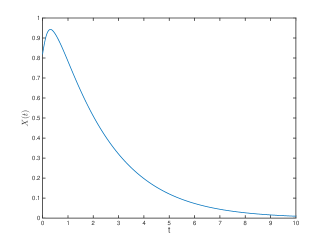
(a) State $X(t)$

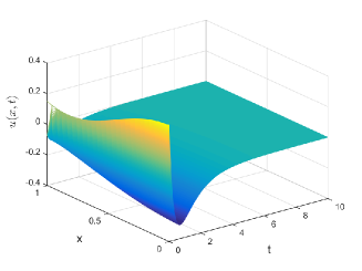
(b) State $u(x,t)$

Figure 1: State when the initial values are chosen inside the ellipsoid $\mathcal{X}_{u}$

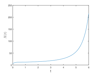
(a) State $X(t)$

(b) State $u(x,t)$

Figure 2: State when the initial values are chosen outside the ellipsoid $\mathcal{X}_{u}$

7 Conclusion

This paper for the first time studied boundary control of PDEs in the presence of saturation. Boundary stabilization of ODE-heat cascade with state time-varying delay was considered. The backstepping method was extended to cascade of systems with state delays. An estimate on the domain of attraction in the presence of actuator saturation was found by using LMIs. Numerical examples illustrated the effectiveness of the proposed design method.

The suggested approach may be extended to cascaded nonlinear ODE-Heat system, where the nonlinear term satisfies the globally Lipschitz condition, and to observer-based control of such a system. The presented method gives efficient tools for various control problems for PDEs with input constraints. These may be the topics for future research.

References

• [1] Curtain, R., Zwart, H.: ‘An introduction to infinite-dimensional linear systems’, (Springer-Verlag, 1995).
• [2] da Silva, J.M.G., Tarbouriech, S.: ‘Antiwindup design with guaranteed regions of stability: an LMI-based approach’, IEEE Trans Automat Control, 50(2005), pp. 106-111.
• [3] El-Farra, N.H., Armaou, A., Christofides, P.D. : ‘Analysis and control of parabolic PDE systems with input constraints’, Automatica, 39(2003), pp. 715-725.
• [4] Fridman, E.: ‘Introduction to Time-Delay Systems: Analysis and Control’, (Basel: Birkhäuser, 2014)
• [5] Fridman, E., Bar Am, N.: ‘Sampled-Data Distributed $H_{\infty}$ Control of Transport Reaction Systems’, SIAM Journal on Control and Optimization, 51 (2013), pp. 1500-1527.
• [6] Fridman, E., Blighovsky, A. :‘Robust sampled-data control of a class of semilinear parabolic systems’, Automatica, 48(2012), pp. 826-836.
• [7] Fridman, E., Orlov, Y.: ‘Exponential stability of linear distributed parameter systems with time-varying delays’, Automatica, 45(2009), pp. 194-201.
• [8] Fridman E., Pila A., Shaked U.: ‘Regional stabilization and $H_{\infty}$ control of time-delay systems with saturating actuators’, International Journal of Robust and Nonlinear Control, 13(2003), pp. 885-907.
• [9] Fridman, E., Solomon, O.: ‘Stability and passivity analysis of semilinear diffusion PDEs with time-delays’, International Journal of Control, 88 (2015), pp. 180-192.
• [10] Halanay, A.: ‘Stability, oscillations, time lags’, (New York: Academic Press).
• [11] Hardy, G.H., Littlewood, J.E., Polya, G.:‘Inequalities’, (Cambridge University Press, Cambridge, UK, 1959).
• [12] Hashimoto, T., Krstic, M.: ‘Stabilization of Reaction Diffusion Equations with State Delay using Boundary Control Input’, IEEE Trans Automat Control, (in press), DOI:10.1109/TAC.2016.2539001.
• [13] Marx, S., Cerpa, E., Prieur, C., Andrieu, V.: ‘Stabilization of a linear Korteweg-de Vries equation with a saturated internal control’, in Proc. European Control Conference, Linz, Austria, 2015, pp. 867-872.
• [14] Krstic, M., Smyshlyaev, A.: ‘Boundary Control of PDEs: A Course on Backstepping Designs’, (Philadelphia, PA: SIAM, 2008).
• [15] Krstic, M.: ‘Compensating actuator and sensor dynamics governed by diffusion PDEs’, Syst. Control Lett., 58(2009), pp. 372-377.
• [16] Krstic, M.: ‘Compensating a string PDE in the actuation or sensing path of an unstable ODE’, IEEE Transactions on Automatic Control, 54(2009) pp.1362–1368.
• [17] Orlov, Y., Dochain, D.: ‘Discontinuous feedback stabilization of minimum-phase semilinear infinite-dimensional systems with application to chemical tubular reactor’, IEEE Trans. Autom. Control, 47(2002), pp. 1293-1304.
• [18] Prieur, C., Tarbouriech, S., da Silva, J.M.G.: ‘Well-posedness and stability of 1D wave equation with saturating distributed input’, in Proc. IEEE Conf. on Decision and Control, Los Angeles, California, USA, 2014, pp. 2846-2851.
• [19] Ren, B.B.,Wang, J.M., Krstic, M.: ‘Stabilization of an ODE-Schrödinger Cascade’, Syst. Control Lett., 62(2013), pp. 503-510.
• [20] Susto. G.A., Krstic, M.: ‘Control of PDE-ODE cascades with Neumann interconnections’, J. Franklin Inst., 347(2010), pp. 284-314.
• [21] Tang, S., Xie, C.: ‘State and output feedback boundary control for a coupled PDE-ODE system’, Syst. Control Lett., 60(2011), pp. 540–545.
• [22] Tarbouriech, S. da Silva, J.M.G.: ‘Synthesis of controllers for continuous-time delay systems with saturating controls via LMI’s, IEEE Transactions on Automatic Control, (45)2000, pp. 105-111.
• [23] Tsubakino, D., Krstic, M., Yamashita, Y.: ‘Boundary control of a cascade of two parabolic PDEs with different diffusion coefficients’, in Proc. IEEE Conf. on Decision and Control, Florence, Italy, 2013, pp. 3720-3725.
• [24] Tucsnak, M. Weiss, G.: ‘Observation and Control for Operator Semigroups’, (Birkhäuser Advanced Texts: Basler Lehrbücher, Birkhäuser Verlag, Basel, 2009).
• [25] Wang, J.M., Liu, J.J., Ren, B.B., Chen, J.H.: ‘Sliding mode control to stabilization of cascaded heat PDE-ODE systems subject to boundary control matched disturbance’, Automatica, 52(2015), pp. 23-34.