Aliasing-truncation Errors in Sampling Approximations of Sub-Gaussian Signals

Abstract

The article starts with new aliasing-truncation error upper bounds in the sampling theorem for non-bandlimited stochastic signals. Then, it investigates $L_{p}([0,T])$ approximations of sub-Gaussian random signals. Explicit truncation error upper bounds are established. The obtained rate of convergence provides a constructive algorithm for determining the sampling rate and the sample size in the truncated Whittaker-Kotel’nikov-Shannon expansions to ensure the approximation of sub-Gaussian signals with given accuracy and reliability. Some numerical examples are presented.

Index Terms: Sampling theorem, truncation error, aliasing error, sub-Gaussian, random process, non-bandlimited.

1 Introduction

Recovering signals from discrete samples and estimating the information loss are the fundamental problems in sampling theory and signal analysis. Whittaker-Kotel’nikov-Shannon (WKS) theorem is a classical tool to recover a continuous band-limited signal from a sequence of its discrete samples. WKS theorems are extensively used in communications and information theory. Various new refine results are published regularly by engineering and mathematics communities, see, e.g., [1, 3, 10, 12, 29] and the recent volumes [13, 23, 30].

A growing body of work uses the sampling reconstruction of stochastic signals to model various real physical processes. However, the sampling theory for the case of stochastic signals is much less developed comparing to its deterministic counterpart. The publications [1, 9, 12, 26, 27] and references therein present an almost exhaustive survey of key approaches in stochastic sampling theory.

The majority of known stochastic sampling results were obtained for harmonizable random processes. Spectral representations of these random processes were used to directly employ the known deterministic sampling results and error bounds for finding mean square approximation errors, see, e.g., [12, 24, 26, 27, 28] among other works. However, in applications, various measures of the closeness of trajectories throughout the entire signal support are often more appropriate than mean-square errors in each time point. Controlling signal distortions in the mean-square sense may result in situations where realizations of stochastic signals are substantially distorted. Instead of small mean-square errors in each location one may need to guarantee that the signal trajectories have not been changed more than a certain tolerance. For example, near-lossless compression requires small user-defined tolerance levels, see [5,11]. It indicates the necessity of elaborating special stochastic techniques.

Another problem is that, in practice, a signal may not have a band-limited spectrum. Recently a considerable attention was given to this problem. One of possible approaches is to use wavelet series representations of stochastic processes, see [17, 18]. Notice that the WKS sampling is an example of such general expansions but requires specific methods and techniques. Another approach to deal with non-bandlimited signals is to simultaneously increase the sampling rate and the sample size used in the truncated WKS formula.

The aliasing error appears due to the divergence between the actual band-region of the spectrum of a signal $\mathbf{X}(t)$ and the assumed one. The aliasing error is defined as the difference between the initial signal $\mathbf{X}(t)$ and its cardinal series expansion, reading as follows:

$$\mathbf{X}(t)-\sum_{k=-\infty}^{\infty}\frac{\sin\left(\omega\left(t-\frac{k\pi}{\omega}\right)\right)}{\omega\left(t-\frac{k\pi}{\omega}\right)}\,\mathbf{X}\left(\frac{k\pi}{\omega}\right).$$ (1)

For stationary stochastic signals a sharp upper bound for the aliasing error was first obtained in [2] and further investigated in [25, 24].

However, in contrast to this theoretical approach, the infinite sum in (1) cannot be employed in numerical implementations as only finitely many samples are available. Hence, one has to estimate the combined aliasing-truncation error

$$\mathbf{X}(t)-\sum_{k=-n}^{n}\frac{\sin\left(\omega\left(t-\frac{k\pi}{\omega}\right)\right)}{\omega\left(t-\frac{k\pi}{\omega}\right)}\,\mathbf{X}\left(\frac{k\pi}{\omega}\right).$$

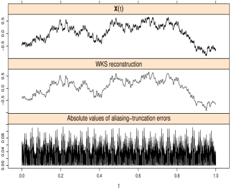
Figure 1: Signal, its WKS reconstruction, and aliasing-truncation error.

The analysis presented in the paper addresses the above problems and contributes to the former stochastic sampling literature. New aliasing-truncation sampling results are derived for the class of sub-Gaussian random processes. This class extends various properties of Gaussian processes to more general settings. The aliasing-truncation error for the WKS expansions has never been studied for sub-Gaussian random processes. Also, a thorough search of the relevant literature only yielded sampling truncation and aliasing results for stochastic signals in the mean-square metric. There are no known truncation and aliasing results on WKS approximations of trajectories of stochastic signals in $L_{p}([0,T])$ metrics in the literature.

Note, that the first progress in studying sampling reconstructions of sub-Gaussian random signals was made in [16]. The authors investigated reconstruction errors of bandlimited signals in $L_{p}([0,T])$ and uniform norms. This paper extends authors’ methodology in [16] to non-bandlimited signals. For the non-bandlimited case it is not enough only to increase the sample size to decrease a reconstruction error. One has to increase both the sampling rate and the sample size. Also, in contrast to the theoretical results in [25, 24], the new approach makes it possible to obtain explicit upper bound estimates which can be used across a range of applications.

The analysis also gives a constructive algorithm for determining sampling rates and sample sizes to ensure the reconstruction of stochastic signals with a given accuracy. The results can be useful in classical applications in communications and information theory and new areas of compressed sensing, see, e.g., [13, 29].

The article proceeds as follows. The next section introduces two classes of sub-Gaussian random processes. Section 2 derives new aliasing-truncation error upper bounds in the WKS approximation of non-bandlimited stochastic signals. Then, Section 4 presents results on the approximation of $\varphi$-sub-Gaussian signals in $L_{p}([0,T])$ with a given accuracy and reliability. Some applications of the obtained results are demonstrated in Section 5. Finally, we conclude the paper with a short discussion and some problems for further investigation.

2 Truncation error upper bounds for non-bandlimited processes

This section presents new truncation error upper bounds in the WKS approximation of non-bandlimited stochastic processes. To the best of the authors’ knowledge the combined aliasing-truncation error has not been studied for stochastic processes, except the weak Cramér class, see [24]. However, the upper bounds in [24] were investigated under additional decay conditions on the family of functions determining stochastic processes. Also these results were not in the explicit form ready for numerical implementations.

Let $\mathbf{X}(t),$ $t\in\mathbf{R},$ be a stationary real-valued mean square continuous random process with $\mathbf{E}\mathbf{\mathbf{missing}}X(t)=0.$ The process $\mathbf{X}(t)$ yields the spectral representation

$$\mathbf{X}(t)=\int_{-\infty}^{\infty}e^{it\lambda}{\rm d}\eta(\lambda),$$

where $\eta(\cdot)$ is a random process with uncorrelated increments. Then, its covariance function is given by

$$\mathbf{B}(\tau):=\mathbf{E}\mathbf{X}(t+\tau)\mathbf{X}(t)=\int_{-\infty}^{\infty}e^{i\tau\lambda}{\rm d}F(\lambda),$$

where $F(\cdot)$ is the spectral function of $\mathbf{X}(t)$ such that $\mathbf{E}\left[\eta(b)-\eta(a)\right]^{2}=F(b)-F(a),$ $b\geq a.$

Let us define the corresponding process $\mathbf{X}_{\Lambda}(t)$ whose spectrum is bandlimited to $[-\Lambda,\Lambda]$ as follows

$$\mathbf{X}_{\Lambda}(t)=\int_{-\Lambda}^{\Lambda}e^{it\lambda}{\rm d}\eta(\lambda).$$

Then, for all $\omega>\Lambda$ there holds

$$\mathbf{X}_{\Lambda}(t)=\sum_{k=-\infty}^{\infty}\frac{\sin\left(\omega\left(t-\frac{k\pi}{\omega}\right)\right)}{\omega\left(t-\frac{k\pi}{\omega}\right)}\,\mathbf{X}_{\Lambda}\left(\frac{k\pi}{\omega}\right),$$ (2)

and the series (2) converges uniformly in mean square.

Let us consider the truncation versions given by the formulae

$$\mathbf{X}_{n}(t):=\sum_{k=-n}^{n}\frac{\sin\left(\omega\left(t-\frac{k\pi}{\omega}\right)\right)}{\omega\left(t-\frac{k\pi}{\omega}\right)}\,\mathbf{X}\left(\frac{k\pi}{\omega}\right),$$ (3)

$$\mathbf{X}_{\Lambda,n}(t):=\sum_{k=-n}^{n}\frac{\sin\left(\omega\left(t-\frac{k\pi}{\omega}\right)\right)}{\omega\left(t-\frac{k\pi}{\omega}\right)}\,\mathbf{X}_{\Lambda}\left(\frac{k\pi}{\omega}\right).$$ (4)

The following result gives a new upper bound for aliasing-truncation errors in the mean square norm.

Theorem 1.

Let $z\in(0,1),$ $t>0,$ and $n\geq\frac{\omega t}{\pi\sqrt{z}}.$ Then

$$\left(\mathbf{E}\left|\mathbf{X}(t)-\mathbf{X}_{n}(t)\right|^{2}\right)^{1/2}\leq A_{n}(t,\Lambda),$$

where

$$A_{n}(t,\Lambda):=\frac{\sqrt{C_{n}(t,\Lambda)}}{n}+D_{n}(t)\cdot\left(\int_{|\lambda|>\Lambda}{\rm d}F(\lambda)\right)^{1/2},$$

$$C_{n}(t,\Lambda):=\mathbf{B}(0)\cdot\left(\frac{4\omega t}{\pi^{2}(1-z)}+\frac{4\left(z+1+\frac{1}{n}\right)}{\pi(1-z)^{2}\left(1-\frac{\Lambda}{\omega}\right)}\right)^{2},$$

$$D_{n}(t):=2+\frac{2\left|\sin(\omega t)\right|}{\pi}\left(1+\mbox{\rm Si}(\pi)+\frac{\frac{\omega t}{\pi}+0.5}{n-\frac{\omega t}{\pi}}\right).$$

For fixed $\omega,$ $t,$ and $z$ the inequality $n\geq\frac{\omega t}{\pi\sqrt{z}}$ provides the sufficient sample size $n$ to guarantee that the mean square reconstruction errors do not exceed the specified level $A_{n}(t,\Lambda).$

Remark 1.

Note that $C_{n}(t,\Lambda)$ is bounded by $C_{1}(t,\Lambda)$ and $D_{n}(t)\leq 2+\frac{2\left|\sin(\omega t)\right|}{\pi}\left(1+\mbox{\rm Si}(\pi)+\frac{\frac{\omega t}{\pi}+0.5}{1-\sqrt{z}}\right).$ Therefore, for fixed $t$, $\omega,$ and $z,$ there is some constant $C,$ for example,

$C=\max\left(C_{1}(t,\Lambda),2+\frac{2\left|\sin(\omega t)\right|}{\pi}\left(1+\mbox{\rm Si}(\pi)+\frac{\frac{\omega t}{\pi}+0.5}{1-\sqrt{z}}\right)\right),$ such that

$$A_{n}(t,\Lambda)\leq C\cdot\left(n^{-1}+\left(\int_{|\lambda|>\Lambda}{\rm d}F(\lambda)\right)^{1/2}\right).$$

Hence, $A_{n}(t,\Lambda)\to 0,$ when both $n$ and $\Lambda$ go to $+\infty.$

Corollary 1.

Let $z^{*}=\frac{\omega^{2}T^{2}}{\pi^{2}n^{2}}\in(0,1),$ $T>0.$ Then

$$\sup_{t\in[0,T]}\left(\mathbf{E}\left|\mathbf{X}(t)-\mathbf{X}_{n}(t)\right|^{2}\right)^{1/2}\leq\tilde{A}_{n}(T,\Lambda),$$

where

$$\tilde{A}_{n}(T,\Lambda):=\frac{\sqrt{\tilde{C}_{n}(T,\Lambda)}}{n}+\tilde{D}_{n}(T)\cdot\left(\int_{|\lambda|>\Lambda}{\rm d}F(\lambda)\right)^{1/2},$$

$$\tilde{C}_{n}(T,\Lambda):=\mathbf{B}(0)\cdot\left(\frac{4\omega T}{\pi^{2}(1-z^{*})}+\frac{4\left(z^{*}+1+\frac{1}{n}\right)}{\pi(1-z^{*})^{2}\left(1-\frac{\Lambda}{\omega}\right)}\right)^{2},$$

$$\tilde{D}_{n}(T):=2+\frac{2}{\pi}\left(1+\mbox{\rm Si}(\pi)+\frac{\frac{\omega T}{\pi}+0.5}{n-\frac{\omega T}{\pi}}\right).$$

3 $\varphi$-Sub-Gaussian random processes

This section reviews the definition of $\varphi$-sub-Gaussian random processes and their relevant properties.

Numerous applications use stationary Gaussian processes. This is justified by the central limit theorem where a resulting process is obtained as a sum of a large number of processes with small variances. However, if summands have relatively large variances the central limit theorem is not applicable and a resulting process may not be Gaussian. At the same time, $\varphi$-sub-Gaussianity often is still a plausible assumption. For example, all centered bounded processes are $\varphi$-sub-Gaussian. Also, sums of independent Gaussian and centered bounded processes are $\varphi$-sub-Gaussian. Moreover, under very mild conditions, the processes admitting the Karhunen-Loéve type expansion are strictly $\varphi$-sub-Gaussian.

The space of $\varphi$-sub-Gaussian random variables was introduced in [19] to generalize sub-Gaussian results from [14] to more general settings. Tail distributions of sub-Gaussian random variables behave similar to the Gaussian ones so that sample path properties of sub-Gaussian processes rely on their mean square regularity. Various properties of $\varphi$-sub-Gaussian random variables were studied in the book [4] and the articles [19, 8]. More information on $\varphi$-sub-Gaussian random processes and their applications can be found in the publications [4, 8, 10] and references therein.

Definition 1.

A continuous even convex function $\varphi(x),$ $x\in{\mathbb{R}},$ is called an Orlicz N-function, if it is monotonically increasing for $x>0$, $\varphi(0)=0,$ ${{\varphi(x)}/{x}}\to 0,$ when $x\to 0,$ and ${{\varphi(x)}/{x}}\to\infty,$ when $x\to\infty.$

Definition 2.

Let $\varphi(x),x\in{\mathbb{R}},$ be an Orlicz N-function. The function $\varphi^{*}(x):=\sup_{y\in{\mathbb{R}}}(xy-\varphi(y)),$ $x\in{\mathbb{R}},$ is called the Young-Fenchel transform of $\varphi(\cdot).$

Definition 3.

An Orlicz N-function $\varphi(\cdot)$ satisfies Condition Q if

$$\lim\limits_{x\rightarrow 0}{\varphi(x)}/{x^{2}}=C>0,$$

where the constant $C$ can be equal to $+\infty.$

Lemma 1.

Let $\varphi(\cdot)$ be an Orlicz N-function. Then it can be represented as $\varphi(u)=\int_{0}^{|u|}f(v)\,dv,$ where $f(\cdot)$ is a monotonically nondecreasing, right-continuous function, such that $f(0)=0$ and $f(x)\to+\infty,$ when $x\to+\infty.$

Let $\{\Omega,\cal{B},P\}$ be a standard probability space and $L_{p}(\Omega)$ denote a space of random variables having finite $p$-th absolute moments.

Definition 4.

Let $\varphi(\cdot)$ be an Orlicz N-function satisfying the Condition Q. A zero mean random variable $\xi$ belongs to the space $Sub_{\varphi}(\Omega)$ (the space of $\varphi$-sub-Gaussian random variables), if there exists a constant $a_{\xi}\geq 0$ such that the inequality $\mathbf{E}\exp\left(\lambda\xi\right)\leq\exp\left(\varphi(a_{\xi}\lambda)\right)$ holds for all $\lambda\in{\mathbb{R}}.$

The space $Sub_{\varphi}(\Omega)$ is equipped the norm (see [4])

$$\tau_{\varphi}\left(\xi\right):=\mathop{\sup}\limits_{\lambda\neq 0}\frac{\varphi^{\left({-1}\right)}\left({\ln\mathbf{E}\exp\left\{{\lambda\xi}\right\}}\right)}{\left|\lambda\right|},$$

where $\varphi^{\left({-1}\right)}(\cdot)$ denotes the inverse function of $\varphi(\cdot).$

If $\varphi(x)={x^{2}}/2$ then the space $Sub_{\varphi}(\Omega)$ is called a space of sub-Gaussian variables. It was introduced in the article [14].

Definition 5.

Let $\mathbf{T}$ be a parametric space. A random process $\mathbf{X}(t),$ $t\in\mathbf{T},$ belongs to the space $Sub_{\varphi}(\Omega)$ if $\mathbf{X}(t)\in Sub_{\varphi}(\Omega)$ for all $t\in\mathbf{T}.$

Gaussian centered random process $\mathbf{X}(t),$ $t\in\mathbf{T},$ belongs to the space $Sub_{\varphi}(\Omega),$ where $\varphi(x)={x^{2}}/2$ and $\tau_{\varphi}(\mathbf{X}(t))=\left(\mathbf{E}\left|\mathbf{X}(t)\right|^{2}\right)^{1/2}.$ If $\mathbf{X}(t)$ is a centered bounded random variable for all $t\in\mathbf{T}$ then the process $\mathbf{X}(t),$ $t\in\mathbf{T},$ belongs to all spaces $Sub_{\varphi}(\Omega).$ Another example is the case when $\mathbf{X}(t)$ is a two-sided Weibull random variable, i.e.

$$\mathbf{P}\left\{{\mathbf{X}(t)}\geq x\right\}=\mathbf{P}\left\{{\mathbf{X}}(t)\leq-x\right\}=\frac{1}{2}\exp\left\{-\frac{x^{\alpha}}{\alpha}\right\},\quad x>0.$$

Then $\mathbf{X}(t),$ $t\in\mathbf{T},$ is a random process from the space $Sub_{\varphi}(\Omega).$

Definition 6.

A family $\Xi$ of random variables $\xi\in Sub_{\varphi}(\Omega)$ is called strictly $Sub_{\varphi}(\Omega)$ if there exists a constant $C_{\Xi}>0$ such that for any finite set $I,$ $\xi_{i}\in\Xi,$ $i\in I,$ and for arbitrary $\lambda_{i}\in{\mathbb{R}},$ $i\in I:$

$$\tau_{\varphi}\left(\sum\limits_{i\in I}\lambda_{i}\xi_{i}\right)\leq C_{\Xi}\left(\mathbf{E}\left(\sum\limits_{i\in I}\lambda_{i}\xi_{i}\right)^{2}\right)^{1/2}.$$

$C_{\Xi}$ is called a determinative constant. The strictly $Sub_{\varphi}(\Omega)$ family will be denoted by $SSub_{\varphi}(\Omega).$

Definition 7.

$\varphi$-sub-Gaussian random process $\mathbf{X}(t),$ $t\in\mathbf{T},$ is called strictly $Sub_{\varphi}(\Omega)$ if the family of random variables $\{\mathbf{X}(t),t\in\mathbf{T}\}$ is strictly $Sub_{\varphi}(\Omega).$ The determinative constant of this family is called a determinative constant of the process and denoted by $C_{\mathbf{X}}$.

A Gaussian centered random process $\mathbf{X}(t),$ $t\in\mathbf{T},$ is a $SSub_{\varphi}(\Omega)$ process, where $\varphi(x)={x^{2}}/2$ and the determinative constant $C_{\mathbf{X}}=1.$

4 Approximation in $L_{p}([0,T])$

This section presents novel results on the WKS approximation of non-bandlimited sub-Gaussian signals in $L_{p}([0,T]),$ $p\geq 1,$ with a given accuracy and reliability. Notice, that the approximation in $L_{p}([0,T])$ provides the closeness of trajectories of the signal $\mathbf{X}(t)$ and its approximant $\mathbf{X}_{n}(t),$ see, e.g., [17, 18]. It is different from the known $L_{p}$-norm results (in particular the mean square results in Section 2) which give only the closeness of distributions for each $t,$ see, e.g., [12, 24, 25].

Theorem 2.

Let $\mathbf{X}(t),$ $t\in\mathbf{R},$ be a stationary $SSub_{\varphi}(\Omega)$ process. Let $\mathbf{X}_{n}(t)$ be defined by (3), $\Lambda\in(0,\omega).$

Then, $\int_{0}^{T}\left|\mathbf{X}(t)-\mathbf{X}_{n}(t)\right|^{p}\,dt$ exists with probability 1 and for any $\varepsilon>S_{n,p}\cdot\left(f\left(p\,(S_{n,p}/\varepsilon)^{1/p}\right)\right)^{p}$ the following inequality holds true

$$\mathbf{P}\left\{\int_{0}^{T}\left|\mathbf{X}(t)-\mathbf{X}_{n}(t)\right|^{p}\,dt>\varepsilon\right\}\leq 2\exp\left\{-\varphi^{*}\left(\left({\varepsilon}/S_{n,p}\right)^{1/p}\right)\right\},$$

where

$$S_{n,p}:=C_{\mathbf{X}}^{p}\int_{0}^{T}A_{n}^{p}(t,\Lambda)\,dt$$

$C_{\mathbf{X}}$ is a determinative constant of the process $\mathbf{X}(t),$ $f$ is from Lemma 1, and $A_{n}(t,\Lambda)$ was defined in Theorem 1.

Remark 2.

It can be seen from Remark 1 that, for fixed $T,$ $\omega,$ and $z,$ we obtain

$$S_{n,p}\leq\tilde{C}\cdot\left(n^{-1}+\left(\int_{|\lambda|>\Lambda}{\rm d}F(\lambda)\right)^{1/2}\right)^{p},$$

where, for example, $\tilde{C}=C_{\mathbf{X}}^{p}\cdot C^{p}\cdot T$ and the constant $C$ is defined in Remark 1.

Hence, $S_{n,p}\to 0,$ when both $n$ and $\Lambda$ go to $+\infty.$

By Remark 2 and Lemma 1 the right hand side of the inequality $\varepsilon>S_{n,p}\cdot\left(f\left(p\,(S_{n,p}/\varepsilon)^{1/p}\right)\right)^{p}$ in Theorem 2 is a decreasing function of $n$ and $\Lambda.$ Hence, for each specific $\varepsilon,$ it gives the sufficient sample size $n$ to guarantee that Theorem 2 holds true.

Example 1.

Let $\varphi(x)={|x|^{\alpha}}/\alpha,$ $1<\alpha\leq 2.$ Then $f(x)=x^{\alpha-1}$ and $\varphi^{*}(x)={|x|^{\gamma}}/\gamma,$ where $\gamma\geq 2$ and $1/{\alpha}+1/{\gamma}=1.$ Hence, the condition of the theorem can be written as

$$\varepsilon>S_{n,p}\cdot\left(f\left(p(S_{n,p}/\varepsilon)^{1/p}\right)\right)^{p}=S_{n,p}^{\alpha}\,p^{(\alpha-1)p}\varepsilon^{1-\alpha}.$$

Therefore, it holds

$$\mathbf{P}\left\{\int_{\mathbf{T}}\left|\mathbf{X}(t)-\mathbf{X}_{n}(t)\right|^{p}\,dt>\varepsilon\right\}\leq 2\exp\left\{-\frac{1}{\gamma}\left(\frac{\varepsilon}{S_{n,p}}\right)^{\gamma/p}\right\},$$

when $\varepsilon>S_{n,p}\cdot p^{\frac{\alpha-1}{\alpha}p}.$

Remark 2 gives a constructive way to select $n$ and $\Lambda$ for a specific tolerance $\varepsilon.$

Recalling that in the Gaussian case $\varphi^{*}(x)=|x|^{2}/2$ we obtain the following specification of Theorem 2.

Example 2.

If $\mathbf{X}(t),$ $t\in\mathbf{R},$ is a Gaussian process, then for $\varepsilon>\hat{S}_{n,p}\cdot p^{p/2}$ it holds

$$\mathbf{P}\left\{\int_{0}^{T}\left|\mathbf{X}(t)-\mathbf{X}_{n}(t)\right|^{p}\,dt>\varepsilon\right\}\leq 2\exp\left\{-\frac{1}{2}\left(\frac{\varepsilon}{\hat{S}_{n,p}}\right)^{2/p}\right\},$$

where

$$\hat{S}_{n,p}:=\int_{0}^{T}A_{n}^{p}(t,\Lambda)\,dt.$$

Definition 8.

$\mathbf{X}_{n}(t)$ approximates $\mathbf{X}(t)$ in $L_{p}([0,T])$ with accuracy $\varepsilon>0$ and reliability $1-\delta,$ $0<\delta<1,$ if

$$\mathbf{P}\left\{\int_{0}^{T}\left|\mathbf{X}(t)-\mathbf{X}_{n}(t)\right|^{p}\,dt>\varepsilon\right\}\leq\delta.$$

Using Definition 8 and Theorem 2 we get the following result.

Corollary 2.

Let $\mathbf{X}(t),$ $t\in\mathbf{R},$ be a stationary $SSub_{\varphi}(\Omega)$ process. Then $\mathbf{X}_{n}(t)$ approximates $\mathbf{X}(t)$ in $L_{p}([0,T])$ with accuracy $\varepsilon$ and reliability $1-\delta$ if the following inequalities hold true

$$\varepsilon>S_{n,p}\cdot\left(f\left(p\,(S_{n,p}/\varepsilon)^{1/p}\right)\right)^{p},$$

$$\exp\left\{-\varphi^{*}\left(\left({\varepsilon}/S_{n,p}\right)^{1/p}\right)\right\}\leq\delta/2.$$

Corollary 3.

If $\mathbf{X}(t),$ $t\in\mathbf{R},$ is a Gaussian process, $\mathbf{X}_{n}(t)$ approximates $\mathbf{X}(t)$ in $L_{p}([0,T])$ with accuracy $\varepsilon$ and reliability $1-\delta$ if

$$\hat{S}_{n,p}<\frac{\varepsilon}{\max\left(p^{p/2},\left(2\ln(2/\delta)\right)^{p/2}\right)}.$$ (5)

5 Applications

This section discusses some practical steps towards applications of the above theoretical results and determining the number of terms in the WKS expansion for specified accuracy and reliability.

The straightforward analysis of the expressions $\tilde{A}_{n}(T,\Lambda),$ $\tilde{C}_{n}(T,\Lambda),$ and $\tilde{D}_{n}(T)$ shows that $\tilde{A}_{n}(T,\Lambda)\to 0$ when $\Lambda$ and $n$ increase to $+\infty$ in such a way that $\Lambda/n\to 0$ and $\Lambda/\omega<1-\rho$ for some constant $\rho\in(0,1).$

The next example demonstrates that the upper bounds in Theorem 1 and Corollary 1 provide a reasonable approximation when the sampling rate and sample size are sufficiently large.

Example 3.

For simulation studies in this example we use signals from the Whittle-Matérn family, see [7, Section 5.2]. Namely, $\mathbf{X}(t)$ has the Whittle-Matérn covariance function with the parameters $\alpha>0,$ $\phi=1,$ and $\nu=1/2$ if

$$\mathbf{B}(\tau)=\sqrt{\frac{{2\pi\tau}}{{\alpha}}}\,K_{\frac{1}{2}}(\alpha\tau),$$

where $K_{\nu}(\cdot)$ is a modified Bessel function of the second kind.

Figure 1 illustrates the WKS reconstruction of this stochastic signal. A simulated realization of the signal $\mathbf{X}(t),$ $t\in[0,1],$ is shown in the upper subplot. The WKS reconstruction $\mathbf{X}_{n}(t)$ and the absolute value of aliasing-truncation errors $|\mathbf{X}(t)-\mathbf{X}_{n}(t)|$ are presented in the lower subplots.

Notice that the spectral density of the signal $\mathbf{X}(t)$ is

$$\frac{{\rm d}F(\lambda)}{{\rm d}\lambda}=\frac{1}{\alpha^{2}+\lambda^{2}},\ \lambda\in\mathbf{R}.$$ (6)

Therefore, the spectrum of the signal $\mathbf{X}(t)$ is non-bandlimited.

The first subplot of Figure 2 demonstrates that for a fixed $\Lambda$ the aliasing-truncation errors are substantial even for large values of $n.$ However, if we increase both $\Lambda$ and $n$ (as it is suggested below) the errors magnitude quickly decreases, see the second subplot in Figure 2. In the both subplots the same $n$ was used.

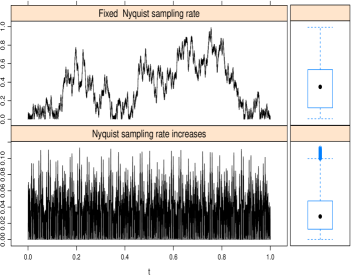
Figure 2: Absolute values of aliasing-truncation errors

Thus, contrary to the case of bandlimited signals, it is not enough to choose a sufficiently large $n$ to get an approximation with given accuracy and reliability. One needs to increase both the number of terms $n$ and the sampling rate $2\Lambda$ simultaneously.

For simplicity, in this numerical example we consider $\omega=2^{N}$ and $\Lambda=3\omega/4,$ i.e. we double the sampling rate by increasing $N$ by 1. For step $N+1$ this choice of sampling rate results in a refined grid formed by dividing the interval between sample values used on step $N.$ Thus, on step $N+1$ one can also use the sampled values from step $N.$ We also select $n=N^{2}\cdot 2^{N}.$ Hence, $n,\Lambda\to+\infty$ and $\Lambda/n\to 0$ when $N\to+\infty.$

Figure 3 demonstrates the difference between the upper bound $\tilde{A}_{n}(T,\Lambda)$ and Monte Carlo estimates of$\sup_{t\in[0,T]}\left(\mathbf{E}\left|\mathbf{X}(t)-\mathbf{X}_{n}(t)\right|^{2}\right)^{1/2}$ obtained by simulating 50 realizations of $\mathbf{X}(t)$ for each $N$. It is clearly seen that the upper bound $\tilde{A}_{n}(T,\Lambda)$ approaches the supremum of mean square aliasing-truncation errors when $N$ increases.

Figure 3: Difference between $\tilde{A}_{n}(T,\Lambda)$ and the true value.

Now we illustrate an application of the results in Section 4 and determine the number of terms in the WKS expansion to ensure the approximation of $\varphi$-sub-Gaussian processes with given accuracy and reliability.

Let $p\geq 1$ in Corollary 3. Then, by Corollary 1, for arbitrary $z\in(0,1)$ and $n\geq\frac{\omega T}{\pi\sqrt{z}},$ we get the following estimate

$$\hat{S}_{n,p}\leq\int_{0}^{T}A_{n}^{p}(t,\Lambda)dt\leq T\tilde{A}_{n}^{p}(T,\Lambda).$$

Hence, to guarantee (5) for given $p,$ $\varepsilon$ and $\delta$ it is enough to choose such $n$ and $\Lambda$ that the following inequality holds true

$$\tilde{A}_{n}(T,\Lambda)\leq\frac{(\varepsilon/T)^{1/p}}{\sqrt{\max\left(p,2\ln(2/\delta)\right)}}.$$ (7)

To apply the obtained results for a specific class of stochastic signals one also needs to estimate the tail behaviour of the spectral function $F(\cdot).$ A widely used statistical approach is based on Abelian and Tauberian theorems, see [21] and references therein. It relies on the fact that the tail behaviour of the spectral function can be found from a local specification of the covariance function in a neighbourhood of zero.

Example 4.

Let $T=B(0)=1,$ and $p=2.$ Similar to Example 3 we choose $\omega=2^{N},$ $\Lambda=3\omega/4,$ and $n=N^{2}\cdot 2^{N}.$ In this example we assume that $\int_{|\lambda|>\Lambda}{\rm d}F(\lambda)\leq\Lambda^{-1}.$ For instance, the signals with spectral densities given by (6) satisfy this condition.

The value of $N$ computed by (7) as a function of $\varepsilon$ and $\delta$ is shown in Figure 4. It is clear that $n$ increases when $\varepsilon$ and $\delta$ approach 0, but for reasonably small $\varepsilon$ and $\delta$ we do not need too many sampled values.

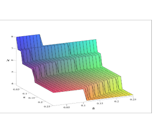
Figure 4: The value of $N$ to ensure specified accuracy and reliability.

For specific values of $\varepsilon,$ $\delta,$ and $p$ the obtained formulae give the sufficient sample size $N$ to guarantee that Theorems 1 and 2 hold true. For example, for fixed $\varepsilon=\delta=0.1,$ Figure 5 illustrates the behaviour of the sufficient sample size as a function of the parameter $p\in(1,2].$

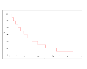
Figure 5: The value of $N$ as a function of $p.$

6 Conclusions

These results may have various applications to approximation problems in signal processing and information theory. The obtained rate of convergence provides a constructive algorithm for determining the sample size and the sampling rate in the WKS expansions to ensure the approximation of $\varphi$-sub-Gaussian signals with given accuracy and reliability. The developed methodology and new estimates are important extensions of the known results in the stochastic sampling theory to the space $L_{p}([0,T])$ and the class of $\varphi$-sub-Gaussian random processes.

It would be of interest

• to apply this methodology to other WKS sampling problems, for example, shifted sampling, irregular sampling, see [24, 25, 26] and references therein;

• to derive analogous results for the multidimensional case and spatial random processes;

• to use approaches in [16] to obtain analogous results in the uniform metric.

Appendix A Proof of Theorem 1

It follows from (2), (3), and (4) that $\mathbf{X}(t)-\mathbf{X}_{n}(t)$ admits the following representation

$$\mathbf{X}(t) - \mathbf{X}_{n}(t)=(\mathbf{X}(t)-\mathbf{X}_{\Lambda}(t))+(\mathbf{X}_{\Lambda}(t)-\mathbf{X}_{{}_{\Lambda},n}(t))$$

$$+ (\mathbf{X}_{\Lambda,n}(t)-\mathbf{X}_{n}(t))=\int_{|\lambda|>\Lambda}e^{it\lambda}{\rm d}\eta(\lambda)$$

$$+ \sum_{|k|\geq n+1}\frac{\sin\left(\omega\left(t-\frac{k\pi}{\omega}\right)\right)}{\omega\left(t-\frac{k\pi}{\omega}\right)}\,\mathbf{X}_{\Lambda}\left(\frac{k\pi}{\omega}\right)$$

$$+ \sum_{k=-n}^{n}\frac{\sin\left(\omega\left(t-\frac{k\pi}{\omega}\right)\right)}{\omega\left(t-\frac{k\pi}{\omega}\right)}\left(\mathbf{X}_{\Lambda}\left(\frac{k\pi}{\omega}\right)-\mathbf{X}\left(\frac{k\pi}{\omega}\right)\right)$$

$$= \int_{-\Lambda}^{\Lambda}\sum_{|k|\geq n+1}e^{i\lambda\frac{k\pi}{\omega}}\,\frac{\sin\left(\omega\left(t-\frac{k\pi}{\omega}\right)\right)}{\omega\left(t-\frac{k\pi}{\omega}\right)}\,{\rm d}\eta(\lambda)$$

$$+ \int_{|\lambda|>\Lambda}\left(e^{it\lambda}-\sum_{k=-n}^{n}e^{i\lambda\frac{k\pi}{\omega}}\,\frac{\sin\left(\omega\left(t-\frac{k\pi}{\omega}\right)\right)}{\omega\left(t-\frac{k\pi}{\omega}\right)}\right){\rm d}\eta(\lambda).$$

Therefore,

$$\left(\mathbf{E}\left|\mathbf{X}(t)-\mathbf{X}_{n}(t)\right|^{2}\right)^{1/2}\leq I_{1}+I_{2}$$

$$=\left(\int_{-\Lambda}^{\Lambda}\left|\sum_{|k|\geq n+1}e^{i\lambda\frac{k\pi}{\omega}}\,\frac{\sin\left(\omega\left(t-\frac{k\pi}{\omega}\right)\right)}{\omega\left(t-\frac{k\pi}{\omega}\right)}\right|^{2}\,{\rm d}F(\lambda)\right)^{1/2}$$

$$+\left(\int_{|\lambda|>\Lambda}\left|e^{i\lambda t}-\sum_{k=-n}^{n}e^{i\lambda\frac{k\pi}{\omega}}\,\frac{\sin\left(\omega\left(t-\frac{k\pi}{\omega}\right)\right)}{\omega\left(t-\frac{k\pi}{\omega}\right)}\right|^{2}{\rm d}F(\lambda)\right)^{1/2}.$$

By Theorem 1 in [16] the first term $I_{1}$ can be bounded as

$$I_{1}^{2}\leq\frac{C_{n}(t,\Lambda)}{n^{2}}.$$ (8)

To estimate the second term $I_{2}$ we use the following bound

$$\left|e^{i\lambda t}-\sum_{k=-n}^{n}e^{i\lambda\frac{k\pi}{\omega}}\,\frac{\sin\left(\omega\left(t-\frac{k\pi}{\omega}\right)\right)}{\omega\left(t-\frac{k\pi}{\omega}\right)}\right|\leq 1+|\sin\left(\omega t\right)|$$

$$\times\left|\sum_{k=-n}^{n}\frac{e^{ik\pi\left(\frac{\lambda}{\omega}+1\right)}}{\omega\left(t-\frac{k\pi}{\omega}\right)}\right|=:1+Z_{n}.$$

Let $k_{t}:=\mbox{nint}\left(\frac{tw}{\pi}\right),$ where $\mbox{nint}(x)$ denotes the integer closest to $x$ (a half integer rounds up), $a:=k_{t}-\frac{\omega t}{\pi}.$ Note that $k_{t}\geq 0$ and $|a|\leq 0.5.$ Then,

$$Z_{n} \leq \left|\frac{\sin\left(k_{t}\pi-\omega t\right)}{k_{t}\pi-\omega t}\right|+|\sin\left(\omega t\right)|\cdot\left|\sum_{\begin{subarray}{c}k=-n\\ k\not=k_{t}\end{subarray}}^{n}\frac{e^{ik\pi\left(\frac{\lambda}{\omega}+1\right)}}{k\pi-\omega t}\right|$$

$$\leq 1+\frac{\left|\sin(\omega t)\right|}{\pi}\cdot\left|\sum_{\begin{subarray}{c}k=-n-k_{t}\\ k\not=0\end{subarray}}^{n-k_{t}}\frac{e^{ik\pi\left(\frac{\lambda}{\omega}+1\right)}}{k+a}\right|$$

$$\leq 1+\frac{\left|\sin(\omega t)\right|}{\pi}\left(\left|\sum_{\begin{subarray}{c}k=-n+k_{t}\\ k\not=0\end{subarray}}^{n-k_{t}}\frac{e^{ik\pi\left(\frac{\lambda}{\omega}+1\right)}}{k+a}\right|\right.$$

$${}+\left.\left|\sum_{k=n-k_{t}+1}^{n+k_{t}}\frac{1}{k-0.5}\right|\right)$$

By $\frac{1}{k+a}=\frac{1}{k}\left(1-\frac{a}{k+a}\right)$ it follows that

$$Z_{n} \leq 1+\frac{\left|\sin(\omega t)\right|}{\pi}\cdot\left(\frac{2|k_{t}|}{n-|k_{t}|+0.5}\right.$$

$${}\left.+\left|\sum_{\begin{subarray}{c}k=-n+k_{t}\\ k\not=0\end{subarray}}^{n-k_{t}}\frac{e^{ik\pi\left(\frac{\lambda}{\omega}+1\right)}}{k}\left(1-\frac{a}{k+a}\right)\right|\right)$$

$$\leq 1+\frac{2\left|\sin(\omega t)\right|}{\pi}\left(\left|\sum_{k=1}^{n-k_{t}}\frac{\sin\left(k\pi\left(\frac{\lambda}{\omega}+1\right)\right)}{k}\right|\right.$$

$${}+\left.\frac{|k_{t}|}{n-|k_{t}|+0.5}+\left|\sum_{\begin{subarray}{c}k=-n+k_{t}\\ k\not=0\end{subarray}}^{n-k_{t}}\frac{a}{2k\left(k+a\right)}\right|\right).$$

The last sum above can be estimated as follows

$$\left|\sum_{\begin{subarray}{c}k=-n+k_{t}\\ k\not=0\end{subarray}}^{n-k_{t}}\frac{a}{2k\left(k+a\right)}\right|=\frac{|a|}{2}\left|\sum_{k=1}^{n-k_{t}}\left(\frac{1}{k\left(k+a\right)}\right.\right.$$

$$\left.\left.+\frac{1}{k\left(k-a\right)}\right)\right|=\frac{1}{2}\left|\sum_{k=1}^{n-k_{t}}\left(\frac{1}{k}-\frac{1}{k+a}+\frac{1}{k-a}-\frac{1}{k}\right)\right|$$

$$\leq\frac{1}{2}\left|\sum_{k=1}^{n-k_{t}}\left(\frac{1}{k-0.5}-\frac{1}{k+0.5}\right)\right|\leq 1.$$

Note that

$$\frac{|k_{t}|}{n-|k_{t}|+0.5}\leq\frac{\frac{\omega t}{\pi}+0.5}{n-\frac{\omega t}{\pi}}.$$

By [22, (3.5.5)] for all $n\in\mathbb{N}$ and $C\in\mathbb{R}$

$$\left|\sum_{k=1}^{n}\frac{\sin(Ck)}{k}\right|\leq\int_{0}^{\pi}\frac{\sin(x)}{x}{\rm d}x=\mbox{Si}(\pi)\approx 1.8519.$$

Therefore we obtain

$$Z_{n}\leq 1+\frac{2\left|\sin(\omega t)\right|}{\pi}\left(1+\mbox{Si}(\pi)+\frac{\frac{\omega t}{\pi}+0.5}{n-\frac{\omega t}{\pi}}\right).$$

Hence,

$$I_{2}^{2}\leq(D_{n}(t))^{2}\cdot\int_{|\lambda|>\Lambda}{\rm d}F(\lambda).$$ (10)

Now, the statement of the theorem follows from (8) and (10).

Appendix B Proof of Theorem 2

In this theorem we investigate the case when $\mathbf{T}=[0,T]$ and $\mu$ is the Lebesgue measure on $[0,T].$ Notice, that it follows from (4) and Definition 6 that $\mathbf{X}(t)-\mathbf{X}_{n}(t)$ is a $SSub_{\varphi}(\Omega)$ random process with the determinative constant $C_{\mathbf{X}}.$

Now, we use the following result from [15].

Lemma 2.

Let $p\geq 1$ and

$$c:=\int_{\mathbf{T}}\left(\tau_{\varphi}(t)\right)^{p}\,d\mu(t)<\infty.$$

Then the integral $\int_{\mathbf{T}}\left|\mathbf{X}(t)\right|^{p}\,d\mu(t)$ exists with probability 1 and the following inequality holds

$$\mathbf{P}\left\{\int_{\mathbf{T}}\left|\mathbf{X}(t)\right|^{p}\,d\mu(t)>\varepsilon\right\}\leq 2\exp\left\{-\varphi^{*}\left(\left({\varepsilon}/c\right)^{1/p}\right)\right\}$$ (11)

for each non-negative

$$\varepsilon>c\cdot\left(f\left(p(c/\varepsilon)^{1/p}\right)\right)^{p},$$ (12)

where $f(\cdot)$ is a density of $\varphi(\cdot)$ defined in Lemma 1.

By the application of Lemma 2 to $\mathbf{X}(t)-\mathbf{X}_{n}(t)$ we obtain that the integral $\int_{0}^{T}\left|\mathbf{X}(t)-\mathbf{X}_{n}(t)\right|^{p}\,dt$ exists with probability 1. In addition,

$$\mathbf{P}\left\{\int_{0}^{T}\left|\mathbf{X}(t)-\mathbf{X}_{n}(t)\right|^{p}\,dt>\varepsilon\right\}\leq 2\exp\left\{-\varphi^{*}\left(\left({\varepsilon}/c\right)^{1/p}\right)\right\},$$

where $c:=\int_{0}^{T}\left(\tau_{\varphi}(\mathbf{X}(t)-\mathbf{X}_{n}(t))\right)^{p}\,dt.$

The functions $\varphi^{*}\left(\cdot\right)$ and $f(\cdot)$ are monotonically non-decreasing. Therefore, due to $S_{n,p}\geq c,$ we obtain

$$S_{n,p}\cdot\left(f\left(p(S_{n,p}/\varepsilon)^{1/p}\right)\right)^{p}\geq c\cdot\left(f\left(p(c/\varepsilon)^{1/p}\right)\right)^{p},$$

$$\exp\left\{-\varphi^{*}\left(\left({\varepsilon}/c\right)^{1/p}\right)\right\}\leq\exp\left\{-\varphi^{*}\left(\left({\varepsilon}/S_{n,p}\right)^{1/p}\right)\right\}.$$

Hence, the statement of Lemma 2 holds true if the constant $c$ is replaced by $S_{n,p},$ which finishes the proof.

Supplementary Materials

The codes used for simulations and examples in this article are available in the folder ”Research materials” from https://sites.google.com/site/olenkoandriy/.

References

• [1] H. Boche, U.J. Monich, ”Approximation of wide-sense stationary stochastic processes by Shannon sampling series,” IEEE Trans. Inf. Theory, vol. 56, no. 12, pp. 6459–6469, Dec. 2010.
• [2] J. L. Brown, ”On mean-square aliasing error in the cardinal series expansion of random processes”, IEEE Trans. Inf. Theory, vol. IT-24, no. 2, pp. 254–256, Mar. 1978.
• [3] P.L. Butzer, P.J.S.G. Ferreira, J.R. Higgins, G. Schmeisser, R.L. Stens, ”The sampling theorem, Poisson’s summation formula, general Parseval formula, reproducing kernel formula and the Paley-Wiener theorem for bandlimited signals ? their interconnections,” Appl. Anal., vol. 90, no.Β 3-4, pp. 431–461, Oct. 2011.
• [4] V.V. Buldygin, Yu.V. Kozachenko, Metric Characterization of Random Variables and Random Processes, American Mathematical Society, Providence R.I., 2000.
• [5] K. Chen, T.V. Ramabadran, ”Near-lossless compression of medical images through entropy-coded DPCM,” IEEE Trans. Med. Imaging, vol. 13, no. 3, pp. 538–548, Sep. 1994.
• [6] P.P.B. Eggermont, V.N. LaRiccia, ”Uniform error bounds for smoothing splines,” in E. GinΓ©, V. Koltchinskii, W. Li, J. Zinn, (Eds.) High Dimensional Probability, IMS Lecture Notes Monogr. Ser., 51, Inst. Math. Statist., Beachwood, OH, 2006, pp. 220–237.
• [7] A.E. Gelfand, P. Diggle, M. Fuentes, P. Guttorp, P. (eds.) Handbook of Spatial Statistics, Chapman & Hall/CRL, Boca Raton, 2010.
• [8] R. Giuliano Antonini, T.-Ch. Hu, Yu. Kozachenko, A. Volodin, ”An application of $\varphi$-subgaussian technique to Fourier analysis,” J. Math. Anal. Appl., vol. 408, no. 1, pp. 114–124, Dec. 2013.
• [9] G. FaΓΏ, S. Kang, ”Average sampling of band-limited stochastic processes,” Appl. Comput. Harmon. Anal., vol. 35, no. 3, pp. 527–534, Jun.Β 2013.
• [10] S.E. Ferrando, R. Pyke, ”Ideal denoising for signals in sub-Gaussian noise,” Appl. Comput. Harmon. Anal., vol. 24, no. 1, pp. 1–13, Apr.Β 2008.
• [11] H. Hartenstein, D. Saupe, ”On entropy minimization for near-lossless differential coding,” IEEE Communications Letters, , vol. 2, no.4, pp. 97–99, Apr. 1998.
• [12] G. He, Z. Song, ”Approximation of WKS sampling theorem on random signals,” Numer. Funct. Anal. Optim., vol. 32, no. 4, pp. 397–408, Mar.Β 2011.
• [13] J.A. Hogan, J.D. Lakey, Duration and Bandwidth Limiting. Prolate Functions, Sampling, and Applications, BirkhΓ€user/Springer, New York,Β 2012.
• [14] J.P. Kahane, ”Properties locales des fonctions a series de Fouries aleatories,” Studia Math., vol. 19, no. 1, pp. 1–25, 1960.
• [15] Yu. Kozachenko, O. Kamenshchikova, Approximation of $\operatorname{SSub}_{\varphi}(\Omega)$ stochastic processes in the space $L_{p}(\mathbb{T})$, Theor. Probab. Math. Statist., vol. 79, pp. 83–88, Dec.Β 2009.
• [16] Yu. Kozachenko, A. Olenko, ”Whittaker-Kotel’nikov-Shannon approximation of $\varphi$-sub-Gaussian random processes,” will appear in J. Math. Anal. Appl., 2016, doi:10.1016/j.jmaa.2016.05.052
• [17] Yu. Kozachenko, A. Olenko, O. Polosmak, ”On convergence of general wavelet decompositions of nonstationary stochastic processes,” Electron. J. Probab., vol. 18, no. 69, pp. 1–21, JulyΒ 2013.
• [18] Yu. Kozachenko, A. Olenko, O. Polosmak, ”Uniform convergence of compactly supported wavelet expansions of Gaussian random processes,” Comm. Statist. Theory Methods, vol. 43, no. 10-12, pp. 2549–2562, MayΒ 2014.
• [19] Yu. Kozachenko, E. Ostrovskyi, ”Banach spaces of random variables of Sub-gaussian type”, Theor. Probab. Math. Statist., vol. 32, pp. 42–53, JuneΒ 1985.
• [20] M.A. Krasnosel’skii, Ya.B. Rutickii, Convex Functions and Orlicz Spaces, Noordhof, GrΓΆningen, 1961.
• [21] N. Leonenko, A. Olenko, ”Tauberian and Abelian theorems for long-range dependent random fields,” Methodol. Comput. Appl. Probab., vol.Β 15, no. 4, pp. 715–742, Dec. 2013.
• [22] D. S. MitrinoviΔ‡, Analytic inequalities, Springer-Verlag, New York-Berlin, 1970.
• [23] K. Moen, H. Ε ikiΔ‡, G. Weiss, E. Wilson, ”A panorama of sampling theory”, in Excursions in harmonic analysis, Vol. 1, BirkhΓ€user/Springer, New York, 2013, pp. 107–127.
• [24] A. Olenko, T. PogΓ‘ny, ”A precise upper bound for the error of interpolation of stochastic processes,” Theor. Probab. Math. Statist., vol. 71, pp.Β 151–163, Dec. 2005.
• [25] A. Olenko, T. PogΓ‘ny, ”Time shifted aliasing error upper bounds for truncated sampling cardinal series,” J. Math. Anal. Appl., vol. 324, no.Β 1, pp. 262–280, Dec. 2006.
• [26] A. Olenko, T. PogΓ‘ny, ”Average Sampling Restoration of Harmonizable Processes,” Comm. Statist. Theory Methods, vol. 40, no. 19-20, pp. 3587–3598, Oct. 2011.
• [27] T. PogΓ‘ny, ”Almost sure sampling restoration of bandlimited stochastic signals,” in Higgins J.R., Stens, R.L. (Eds.) Sampling Theory in Fourier and Signal Analysis: Advanced Topics, Oxford University Press, Oxford, 1999, pp. 203–232, 284–286.
• [28] Z. Song, B. Liu, P. Yanwei, H. Chunping, L. Xuelong, ”An improved Nyquist-Shannon irregular sampling theorem from local averages”, IEEE Trans. Inf. Theory, vol. 58, no. 9, pp. 6093–6100, Sept.Β 2012.
• [29] L. Xue, H. Zou, ”Sure independence screening and compressed random sensing,” Biometrika, vol. 98, pp. 371–380, JuneΒ 2011.
• [30] A.I. Zayed, G. Schmeisser, (Eds.) New Perspectives on Approximation and Sampling Theory. Festschrift in Honor of Paul Butzer’s 85th Birthday, BirkhΓ€user/Springer, New York, 2014.