On Information-Theoretic Characterizations of Markov Random Fields and Subfields
Abstract
Let form a Markov random field (MRF) represented by an undirected graph , and be a subset of . We determine the smallest graph that can always represent the subfield as an MRF. Based on this result, we obtain a necessary and sufficient condition for a subfield of a Markov tree to be also a Markov tree. When is a path so that form a Markov chain, it is known that the -Measure is always nonnegative and the information diagram assumes a very special structure [11]. We prove that Markov chain is essentially the only MRF such that the -Measure is always nonnegative. By applying our characterization of the smallest graph representation of a subfield of an MRF, we develop a recursive approach for constructing information diagrams for MRFs. Our work is built on the set-theoretic characterization of an MRF in [15].
Key Words: -Measure, conditional independence, Markov random field, subfield, Markov tree, Markov chain, information diagram.
1 Introduction
A Markov random field (MRF) is often regarded as a generalization of a one-dimensional discrete-time Markov chain in the sense that the time index for the latter is replaced by a space index for the former. Historically, the study of MRFs stems from statistical physics. The classical Ising model, which is defined on a rectangular lattice, was used to explain certain empirically observed facts about ferromagnetic materials. In statistics, the dependencies between variables in a contingency table may also be modeled as an MRF [7]. In image processing and computer vision, the dependencies between pixels or image features are also commonly modeled by MRFs [21]. MRFs have also been used in wireless and ad hoc networking [17, 20, 19]. In recent years, MRFs have been used as a model for studying social networks [22, 23] and big data [24].
The foundation of the theory of MRFs may be found in [5] or [3] (also see [6] and [13]). It was described in [5] that the theory can be generalized to the context of an arbitrary graph. In this paper, we discuss such MRFs whose random variables are discrete. Before we present their formulation, we first introduce some notations that are used throughout the paper.
In this paper, all random variables are discrete. Let be a random variable taking values in an alphabet . The probability distribution for is denoted as , with . When there is no ambiguity, is abbreviated as . The support of , denoted by , is the set of all such that . If , we say that is strictly positive, denoted by . Otherwise, contains zero probability masses, and we say that is not strictly positive. Note that probability distributions with zero probability masses are in general very delicate, and they need to be handled very carefully (see Example 1 below). All the above notations naturally extend to two or more random variables.
Proposition 1.
For random variables , and , if and only if
| (1) |
for all , , and such that , where is some function of and and is some function of and .
The example below illustrates the subtlety of conditional independence when the probability distribution contains zero probability masses.
Example 1.
Let denote the joint distribution of three random variables , and . In this example, we show that
| (2) |
holds if , but does not hold in general.
Assume that . Then for all , and , by , we have
| (3) |
and by , we have
| (4) |
Then
or
Substituting this into (4), we have
i.e., .
However, (2) does not hold in general, because if , we see that and but . Note that is not strictly positive if .
We now present the formulation of an MRF defined on an arbitrary graph. Let be an undirected graph, where is the set of vertices and is the set of edges. We assume that there is no edge in which joins a vertex to itself. For any (possibly empty) subset of , denote by the graph obtained from by removing all the vertices in and all the edges joining a vertex in . Let be the number of components111 A component of an undirected graph is a subgraph in which any two vertices are connected, and which is not connected to any additional vertices in the supergraph. in . Denote the sets of vertices of these components by . If , we say that is a cutset in . Throughout this paper, whenever we remove a subset of vertices from , we always assume that we also remove all the edges joining a vertex in .
Consider a collection of random variables whose joint distribution is specified by a probability measure on , where random variable is associated with vertex in graph . We now define a few Markov properties for random variables pertaining to a graph :
Definition 1 (Pairwise Markov Property).
For all distinct such that , and are independent conditioning on .
Definition 2 (Local Markov Property).
For all , and are independent conditioning on , where is the set of neighbors of vertex and .
Definition 3 (Global Markov Property).
Let be a partition of such that the sets of vertices and are disconnected in . Then the sets of random variables and are independent conditioning on .
Proposition 2.
Random variables satisfy the global Markov property if and only if for all cutsets in , the sets of random variables are mutually independent conditioning on .
See [15] for a proof of Proposition 2. When , this proposition states that if the graph has more than one component, i.e., , then the sets of random variables are mutually independent. Here we regard unconditional mutual independence as a special case of conditional mutual independence.
Denote the Pairwise Markov Property, the Local Markov Property, and the Global Markov Property by (P), (L), and (G), respectively. It can readily be seen from their definitions that (G) (L) (P).
Definition 4 (Markov Random Field).
The probability measure , or equivalently, the random variables , are said to form an MRF represented by a graph if and only if the Global Markov Property is satisfied by .
If form an MRF represented by a graph , we also say that form a Markov graph , are represented by , or is a (graph) representation for . When is a path,222A path is a graph whose vertices can be linearly ordered so that every pair of consecutive vertices forms an edge. we say that form a Markov chain. When is a tree, we say that form a Markov tree.333The term “Markov tree” is also used in the number theory literature in the context of the Markov number, but it is not to be confused with the Markov tree in this paper. When is a cycle graph,444A cycle graph is a graph that consists of a single cycle. we say that form a Markov ring.
In general, can be represented by more than one graph. In particular, are always represented by , the complete graph with vertices. The graph specifies a degenerate MRF, because for every , is not a cutset in . In other words, no Markov constraints are imposed on by .
Suppose the random variables are represented by both and , where , i.e., is a proper subgraph of . Then imposes a larger set of Markov constraints on than , because a cutset in is also a cutset in (but not vice versa). Thus we are naturally interested in the “smallest” graph (to be discussed in Section 2.4) that represents .
Definition 5 (Subfield).
A subset of the random variables forming an MRF is called a subfield of the MRF.
Definition 6.
A -tuple is called a configuration. A probability measure on is strictly positive, denoted by , if for all configurations .
If , it can be shown that (G) = (L) = (P) (see for example [13]). In general, however, a probability measure may contain zero probability masses, i.e., for some configuration . For example, if some random variables in are functions of other random variables, then is not strictly positive.
In this paper, we study the structure of MRFs by means of an information-theoretic approach. Specifically, structural properties of MRFs are obtained through the investigation of the set-theoretic structure of Shannon’s information measures under the constraints imposed by the MRF. With this approach, we do not have to manipulate the underlying probability measure directly.
An identity involving only Shannon’s information measures (i.e., entropy, mutual information, and their conditional versions) is referred to as an information identity. The set-theoretic structure of Shannon’s information measures was first studied in [1], where it was proved that for every information identity, there is a corresponding set identity. This was further developed into the theory of -Measure in [9]. Under this framework, every Shannon’s information measure can formally be regarded as the value of a unique signed measure called the -Measure, denoted by , on a set corresponding to that Shannon’s information measure. This establishes a complete set-theoretic interpretation of Shannon’s information measures.
Subsequent to [9], the structure of the -Measure for a Markov chain and more generally an MRF was investigated in [11] and [15], respectively. In particular, it was proved in [11] that the -Measure for a Markov chain is always nonnegative, and an information diagram that displays the special structure of the -Measure for a Markov chain was obtained.
The current work, consisting of the following three main results, is built on [1, 9, 11, 15]:
-
1.
Let be any set of random variables that form an MRF represented by a graph , and let , where , be any subfield of the MRF. We determine the smallest graph that can always represent .
-
2.
The -Measure of an MRF is always nonnegative if and only if the MRF is represented by either a path or a forest of paths.555A forest of paths is a graph with at least two components such that each component is a path.
-
3.
We develop a recursive approach for constructing an information diagram that displays the special structure of the -Measure for an MRF.
The rest of the paper is organized as follows. Section 2 contains an overview of the concepts and tools to be used in this paper. In Section 3, we define the graph and establish that is the smallest graph that can always represent the subfield . Applying this result to Markov trees, we obtain in Section 4 a necessary and sufficient condition for a subfield of a Markov tree to form a Markov subtree. In Section 5, we establish that Markov chains are essentially the only MRFs for which the -Measure is always nonnegative. In Section 6, we develop a recursive approach for constructing an information diagram that displays the special structure of the -Measure for an MRF. The paper is concluded in Section 7.
2 Preliminaries
In this section, we introduce the notations and present the preliminaries for the rest of the paper. For a detailed discussion, we refer the readers to [18, Chapters 3 and 12] and the references therein.
2.1 -Measure
We first give an overview of the basics of the -Measure. Let be jointly distributed discrete random variables, and be a set variable corresponding to a random variable . We note that the -Measure does not have to be defined in the context of an MRF, but here we use (the vertex set of a graph) as the index set of the random variables for the sake of convenience. Here we assume that for , so that the -Measure [9] for is well-defined.
Define the universal set to be and let be the -field generated by . The atoms of have the form , where is either or . Let be the set of all the atoms of except for , which is equal to the empty set because
Note that . In the rest of the paper, when we refer to an atom of , we always mean an atom in unless otherwise specified.
To simplify notation, we will use to denote and to denote for any . We will not distinguish between and the singleton containing . It was shown in [9] that there exists a unique signed measure on which is consistent with all Shannon’s information measures via the following substitution of symbols:
| , | ||||
| ; | ||||
where “” denotes the set difference. For example,
For all , is a linear combination of for nonempty subsets of .
2.2 Full Conditional Mutual Independency
Definition 7.
Let be a partition of , where and . The tuple defines the following conditional mutual independency (CMI) on :
If , is called a full conditional mutual independency (FCMI).
Example 2.
For , defines the FCMI
However, for , is not an FCMI because is not a partition of .
Definition 8.
Let be an FCMI on . The image of , denoted by , is the set of atoms of of the form
| (5) |
where , , and there exist at least two such that .
The following proposition gives a more explicit expression for . The proof is elementary and so is omitted.
Proposition 3.
Let be an FCMI on . Then
In the rest of paper, we denote the atom of by , etc.
Example 3.
The following theorem from [18] will be useful for proving some of the results in this work.
Theorem 1.
Let be an FCMI on . Then holds if and only if for all .
Thus the effect of an FCMI on the joint probability distribution of is completely characterized by . We remark that if is a partition of where , then holds if and only if vanishes on all the sets prescribed in (5), although these sets are no longer atoms of .
Example 4.
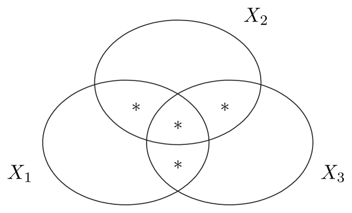
Following Example 3, the random variables , and are mutually independent if and only if vanishes on the atoms , , , and .
Let be a nonempty atom of . Define the set
| (6) |
Note that is uniquely specified by because
Also note that in the definition of , its dependence on is implicit, and what the set is should be clear from the context.
Define as the weight of the atom , the number of in which are not complemented. We now show that an FCMI is uniquely specified by . First, by letting for in (5), we see that the atom
is in , and it is the unique atom in with the largest weight. From this atom, can be determined. To determine , we define a relation on as follows. For , is in if and only if one of the following is satisified:
-
i)
;
-
ii)
and the atom
(7) is not in .
The idea of ii) is that is in if and only if for some , which can be seen as follows. If for some , then the atom in (7) is not in by Definition 8 because and so but for all (an atom in has at least two such that ). On the other hand, if and where , then by letting and , we see that the atom in (7) is in .
Then is reflexive by i), and is symmetric because the definition of is symmetrical in and . Moreover, is transitive from the discussion above because if for some and for some , then and . In other words, is an equivalence relation that partitions into . Therefore, can be recovered from , and so it is uniquely specified by .
Let be a collection of FCMIs on , and define
Since holds if and only if holds for all , it follows from Theorem 1 that holds if and only if for all . Thus the effect of a collection of FCMIs on the joint probability distribution of is completely characterized by .
Consequently, for two collections and of FCMIs, if and only , and if and only .
One can interpret as the “footprint” of an FCMI . Then the footprint of a collection of FCMIs is simply the union of the footprints of the individual FCMIs in . However, two different collections of FCMIs may have the same footprints, as shown in the next example. Thus unlike an FCMI, a collection of FCMIs is in general not uniquely specified by its image.
Example 5.
Let . Let and , where
Then but .
2.3 Markov Random Field
In the definition of an MRF, each cutset in specifies an FCMI on , denoted by . Formally,
| conditioning on . |
Then in light of (6), for such that , is the FCMI induced by the cutset . It follows that form a Markov graph if and only if
| (8) |
where ‘’ denotes ‘logical AND’. This is the collection of FCMIs induced by graph .
Definition 9.
Let be a graph. For an atom of , if , i.e., is connected, then is a Type I atom of , otherwise, i.e., , is a Type II atom of . The sets of all Type I and Type II atoms of are denoted by and , respectively.
Definition 10.
For a graph , the image of is defined by
Theorem 2.
(cf. [18, Theorem 12.25]) .
The above theorem gives a precise characterization of . It follows from the discussion in Section 2.2 that form a Markov graph if and only if for all , i.e., vanishes on all the Type II atoms of .
Example 6.
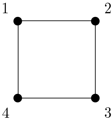
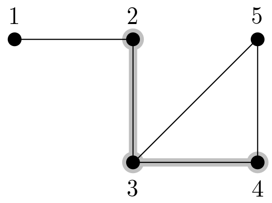
For the cycle graph in Fig. 2, . Random variables and are represented by if and only if .
A graph and the collection of FCMIs it induces uniquely specify each other, because for distinct , if and only if the FCMI is not in . This can be seen as follows. If , then is not a cutset in , and so . On the other hand, if , then is not a cutset in , which implies .
Although a collection of FCMIs is in general not uniquely determined by its image (cf. Example 5), the following proposition asserts that a graph (and hence ) is uniquely determined by its image .
Proposition 4.
For a graph , if and only if the atom
| (9) |
is not in .
Proof Denote the atom in (9) by . If , then induces the FCMI . Obviously, , and hence .
To prove the converse, assume that atom A is in , and specifically in some such that . It follows from Definition 8 that in order for to be in , it is necessary for and to be in different sets in . This implies that is a cutset in , and hence .
With this proposition, a graph can be recovered from as follows. Start with the complete graph . If there exists an atom in as prescribed by (9) for some distinct , then remove edge from the graph. Repeat this step until no more edges can be removed. Note that this algorithm produces a unique graph, i.e., . As a corollary, the uniqueness of the Markov graph induced by is proved, i.e., for two graphs and where , .
2.4 Smallest Graph Representation
As discussed in Section 1, we are interested in the “smallest” graph that can represent a given set of random variables . To fix ideas, we first give a formal definition of this notion.
Definition 11.
A graph is the smallest graph representation for a set of random variables if is a representation for and is a subgraph of any representation for .
We know from Section 2.3 that a graph can represent if and only if vanishes on all the atoms in . Note that if is a subgraph of , then a cutset in is also a cutset in . It follows that is a “subset” of , and hence .
For the given set of random variables , let be the set of nonempty atoms of on which vanishes. Following the last paragraph, if is the smallest representation for , then and for any representation for . The next theorem gives a characterization of such a graph if it exists.
Theorem 3.
For a given set of random variables , let be the set of nonempty atoms of on which vanishes. Let be such that if and only if the atom in (9) is not in . Then if the smallest graph representation for exists, it is equal to .
We first prove the following two lemmas.
Lemma 1.
Every graph that can represent contains as a subgraph.
Proof Let be any graph that can represent . Consider any edge in , i.e., . By construction, the atom in (9) is not in . Then , otherwise the FCMI holds, i.e.,
which is a contradiction because the atom in (9) is not in . Thus if can represent , then contains as a subgraph.
Lemma 2.
If is an edge in every graph that can represent , then is an edge in .
Proof Let be an edge in every graph that can represent . If a graph does not contain , then it cannot represent . In particular, the graph obtained by removing from the complete graph cannot represent . Since the only FCMI imposed by is (i.e., and are independent conditioning on ), this means that and are not independent conditioning on , or . In other words, the atom is not in , which implies that is an edge in .
Proof of Theorem 3 Assume the smallest graph representation for exists and let it be . By Lemma 1, is a subgraph of . On the other hand, since is a subgraph of every graph that can represent , Lemma 2 implies that is a subgraph of . Hence, .
Corollary 1.
The smallest graph representation for exists if and only if is a representation for .
Proof Assume that the smallest graph representation for exists. By Theorem 3, it is equal to , and so is a representation for . Conversely, if is a representation for , then by Lemma 1, it is the smallest representation for .
Example 7.
The above example shows that the smallest graph representation may not exist for a given set of random variables. However, if for some graph , then is in fact the smallest graph representation for . This is proved in the next proposition.
Proposition 5.
If for some graph , then is the smallest graph representation for .
Proof We see that a graph can be recovered from its image using the algorithm described at the end of Section 2.3, and in fact . Therefore, , which implies that . Hence, is a graph representation for . It then follows from Theorem 3 that , i.e., , is the smallest graph representation for .
To our knowledge, Corollary 1 is new. A related result can be found in [8], where it was proved that if the underlying probability measure is strictly positive, then the smallest graph representation for always exists and is equal to .
Example 8.
In Example 7, the constraint (10) is equivalent to and , while consists of the FCMIs
We have shown in Example 1 that
holds if the underlying probability distribution is strictly positive, or , but does not hold in general. This means that if , then represents , and , but in general it does not. These conclusions are consistent with the result in [8] and the discussion in Example 7, respectively.
3 Subfield of a Markov Random Field
Let form an MRF represented by some graph . Note that such a graph can always be found, because is always a representation of . Let be a subset of . In this section, we seek the smallest graph that can always represent the subfield .
Definition 12.
Let and where . If , we write .
Let form an MRF represented by a graph . Following the definition above, if , then form an MRF represented by .
Definition 13.
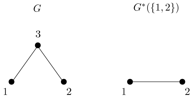
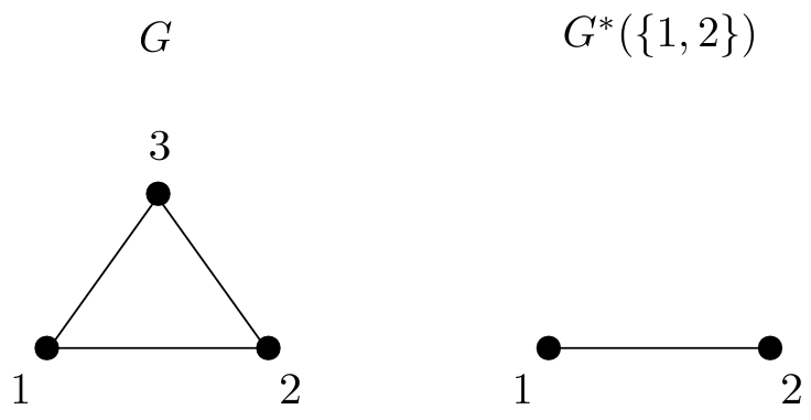
Let , and let . Let be such that for distinct , if and only if there exists a path between and in on which all the intermediate vertices are in .
Obviously, . We will prove in Theorem 8, the main theorem of this section, that is the smallest such that .
Example 9.
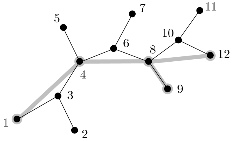
Consider an MRF represented by the graph in Fig. 4, which indeed is a Markov chain. Let . Then is illustrated as the overlay graph in grey.
Example 10.
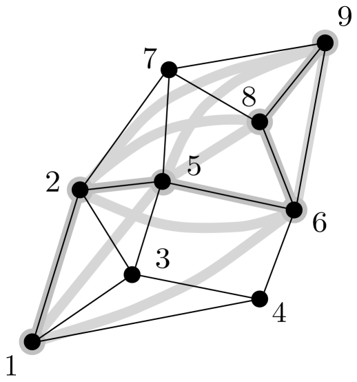
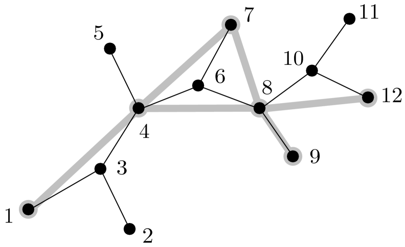
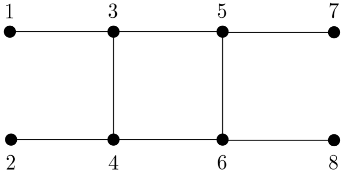
Consider an MRF represented by the more elaborate graph in Fig. 5. Let . Then is illustrated as the overlay graph in grey.
Consider . The next proposition asserts that can be obtained in two steps. First obtain from by applying Definition 13. Then obtain from by applying Definition 13 again with in place of .
Proposition 6.
Let and . Then .
Proof See Appendix A.
Consider , where
For distinct , if , then by the definition of . In other words, always contains as a subgraph. However, in general. In other words, is not necessarily a subgraph of . The following proposition gives the condition for to be exactly equal to .
Proposition 7.
Let , and let . Let be the set of elements of such that some of their neighbors are in , i.e.,
| (11) |
Then if and only if for distinct , if is not an edge in , then there exists no path between and in on which all the vertices other than and are in .
Proof Note that is equivalent to . We already have proved that always holds, so we only need to prove that the condition in the proposition for is necessary and sufficient for .
For any distinct , consider two cases. If either or is not in , then implies . If both and are in , then the condition in the proposition for is necessary and sufficient for to imply . The proposition is proved.
Example 11.
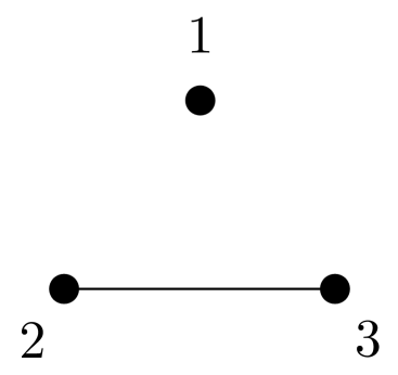
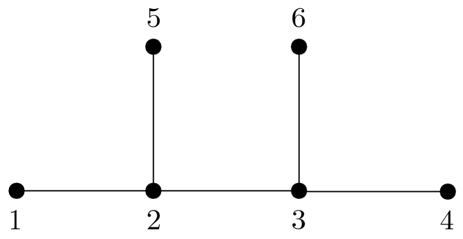
Consider the graph in Fig. 6 and let . Here because each vertex in is connected to some vertex in . Now is the only pair of vertices that is not an edge in . Since there exists no path between vertices 2 and 4 on which all the vertices other than 2 and 4 are in , by Proposition 7, , which is illustrated as the overlay graph in grey.
Corollary 2.
Let and , where . Let be represented by a graph such that and is the only neighbor of . Then is represented by .
Proof This is a special case of Proposition 7 with .
As discussed above, always contains as a subgraph. The next theorem gives an alternative characterization of that describes the relation between and more explicitly. For , let
be the set of neighbors of in graph ,666Note that , where is defined in (11). and
be the set of edges of the clique formed by the vertices in .
Theorem 4.
Let . For , let and . Then
| (12) |
where are the components of .
Proof To facilitate our discussion, let denote the set on the right hand side of (12). We first prove that . By Definition 13, if , then there exists a path between and in on which all the intermediate vertices are in . Denote this set of vertices in by . If , then we have . Otherwise, since the vertices in are connected in , is a subset of for some . As such, and hence . This completes the proof for .
It remains to prove that . Let . If , then because as discussed. If for for some , then , i.e., there exists ( and are not necessarily distinct) such that . Since and are in the same component of , namely , they are connected and it follows that there exists a path between and in on which all the intermediate vertices are in . Therefore, and we conclude that . The theorem is proved.
Corollary 3.
In Theorem 4, if , then
Proof If suffice to observe that forms the only component of .
Theorem 5.
If , then if there exists a path between and in on which all the intermediate vertices are in .
Proof Consider distinct such that there exists a path between and in on which all the intermediate vertices are in . Denote this set of vertices in by . Consider
| (13) |
Since , we see that
is one of the atoms in the union in (13). Note that because , , and the vertices in form a path in . Thus is a Type I atom for .
Now construct by letting
where is a random variable such that . Then by the proof of Theorem 3.11 in [18], for all ,
Now for so constructed, vanishes on all the Type II atoms of because , the only atom on which does not vanish, is a Type I atom. Then from the discussion following Theorem 2, we see that satisfy . On the other hand, in light of (13), we have
i.e., and are not independent conditioning on . Hence, for any , if , then is not a cutset in , which implies that . The theorem is proved.
Theorem 6.
If , then contains as a subgraph.
Theorem 7.
.
Proof Let be any set of random variables which satisfy . We need to prove that satisfy . For a fixed cutset in , let be the number of components in and denote these components by . To prove that satisfy , it suffices to prove that for every cutset in , are mutually independent conditioning on .
Note that is a partition of . Following the discussion immediately after Theorem 1, we see that it suffices to prove that vanishes on the sets prescribed in (5). The atoms of contained in a set prescribed in (5) have the form
| (14) |
where , , , and there exist at least two such that .
We will prove that every atom prescribed in (14) is a Type II atom of . Since satisfy , vanishes on these atoms. It then follows that
i.e., vanishes on the sets prescribed in (5), as is to be proved.
To prove that the atom in (14) is a Type II atom of , we need to show that is a cutset in . Now in (14), let be such that and are nonempty, and let and .We claim that and are disconnected in . Assume the contrary is true, i.e., there exists a path between and in . First of all, both and are in and they belong to different components in . Since , the vertices between and on this path are either in or . Then on this path (including and ) there exists two distinct vertices and in such that
-
1)
and are in different components in ;
-
2)
all the vertices between and on the path are in
(it is possible that and ). Then 2) above implies that is an edge in (cf. Definition 13), which is a contradiction to 1). Therefore, we conclude that and are disconnected in . Hence has at least two components and is a cutset in . This completes the proof of the theorem.
The following corollary gives a structural property of .
Corollary 4.
If is a cutset in , then is also a cutset in .
Proof In the proof of Theorem 7, we have proved that if is a cutset in , then is a cutset in . By setting and for all , this cutset becomes . This proves the corollary.
Theorem 8.
Let , and let . Then is the smallest such that .
We end this section with a discussion. There has been much research along the line of MRFs in the field of graphical models [25]. In particular, classes of graphical models that contain undirected graph as a special case were defined in [26, 27], where a separation criterion was provided for which the class of graphical models is stable under marginalization. In the context of the present paper, their result can be described as follows. Let be an undirected graph and . In [26, 27], an algorithm is provided that takes as the input and produces a graph as the output which is essentially the same as , and it was shown that if satisfy only those conditional independencies induced by (i.e., satisfy the conditional independencies induced by and no more), then satisfy only those conditional independencies induced by . This implies that if , then cannot be a subgraph of , i.e., Theorem 8.
Although the graph produced by the algorithm in [27] is essentially the same as , it is not given in closed form. By contrast, our closed-form characterizations of (Definition 13, Theorem 4, and Corollary 3) facilitate the development of further results, including Proposition 6 and the recursive approach for constructing information diagrams for MRFs to be discussed in Section 6.
It is also worth pointing out that our proof of Theorem 8, which is information-theoretic, is interesting on its own because it is developed upon the view that an MRF is a collection of FCMIs. As such, some of the results in this paper can potentially be generalized for general collections of FCMIs, which is beyond the scope of graphical models.
4 Markov Tree
Suppose are represented by a graph . If is a tree, then form a Markov tree. If is also a tree, we say that form a Markov subtree. For the special case when is a path, it is easy to see that is always a path (see Example 9 for instance). In other words, if form a Markov chain, then for any , always form a Markov subchain.
However, if form a Markov tree, for an arbitrary subset of , may or may not form a Markov subtree. The following theorem, which is an application of Theorem 8, gives a necessary and sufficient condition for to form a Markov subtree.
Theorem 9.
Let form an MRF represented by a tree . For , is a tree if and only if there do not exist and such that for , all the vertices on the path between and except for are in .
Proof We first prove the “only if” part. Assume that is a tree and there exist and and such that for , all the vertices on the path between and except for are in . By Definition 13, the edges , , and are in . Hence form a cycle in , a contradiction to the assumption that is a tree.
We now prove the “if” part. Assume that is not a tree. Then there exists a cycle in , where and are distinct. By Definition 13, for each , there exists a path between and in on which all the intermediate vertices are in , where ‘+’ in the subscript denotes modulo addition. This path is in fact unique because is a tree, so we denote it by Path.
If all the vertices on the collection of paths Path, , except for the endpoints, are distinct, since are distinct, these paths together form a cycle in which is a contradiction because is a tree. Otherwise, there exists a vertex which is on both Path and Path for some . Note that , with equality if and only if . Then there exist such that for , all the vertices on the path between and except for are in . The theorem is proved.
5 Markov Chain
A Markov chain is a special case of a Markov tree. However, there are certain properties that are possessed by a Markov chain but not by a Markov tree in general. Consider the graph , where and the edges in are for . Evidently, is a path. If is represented by , then form the Markov chain . The following properties of a (finite-length) Markov chain were proved in [11]:
-
(C1)
An atom of is a Type I atom if and only if
(15) where , i.e., the indices of the set variables in that are not complemented are consecutive.
-
(C2)
The values of on all the Type I atoms are nonnegative.
-
(C3)
vanishes on all the Type II atoms.
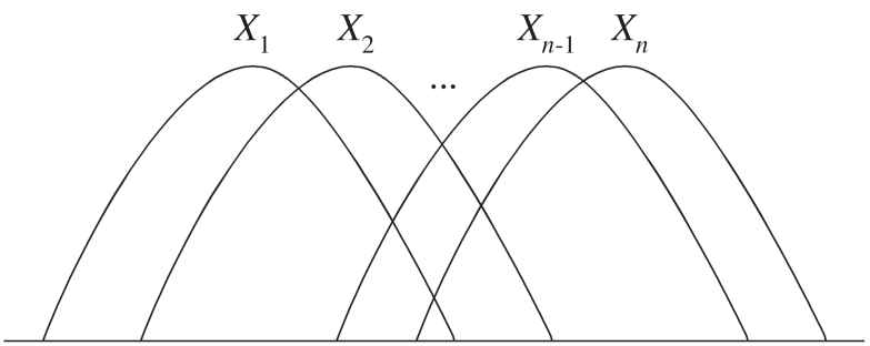
Since vanishes on all the Type II atoms and is nonnegative on all the Type I atoms, it is a measure on . Also, the -Measure of a finite-length Markov chain can be represented by a 2-dimensional information diagram as in Fig. 9, in which all the Type II atoms are suppressed.
Subsequently, (C3) was generalized for arbitrary finite undirected graphs [15]. However, the nonnegativity of the -Measure does not hold even for the simplest Markov tree that is not a Markov chain [15].
Example 14.
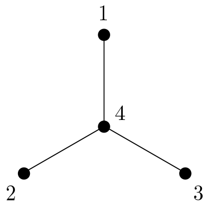
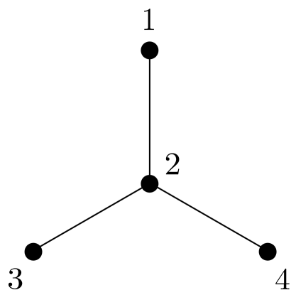
Let and be i.i.d. random variables each distributed uniformly on . Let , , , and . Since , , and are functions of , they are mutually independent conditioning on . Thus , and form a Markov tree represented by the “star” in Figure 10. It is not difficult to show that (see [18, Example 3.10])
and hence is not nonnegative.
Before explaining the significance of the nonnegativity of for Markov chains, we first review the following result in [11] which is instrumental in proving the nonnegativity of for a Markov chain. Prior to [11], the same result (and also the converse) was proved in [1] for the special case .
Lemma 3.
If form a Markov chain, then for a Type I atom with defined in (15),
| (16) |
Note that the first equality above follows directly from the definition of , and the quantity on the right hand side is equal to which is always nonnegative. In other words, Lemma 16 asserts that the values of on all the Type I atoms are nonnegative. Therefore, is a measure.
As mentioned in Section 2.1, for all , is a linear combination of for nonempty subsets of . Then if forms a Markov chain, any linear information inequality involving can be expressed in the form
where . The following theorem gives a complete characterization of such inequalities that always holds.
Theorem 10.
If forms a Markov chain, then
| (17) |
always holds if and only if for all .
Proof If forms a Markov chain, then for all . If for all , then evidently (17) always holds.
To prove the converse, assume that for an atom . Now construct by letting
where is a random variable such that . Then by the proof of Theorem 3.11 in [18], for all ,
It follows that
since and . Hence, (17) does not always hold and the converse is proved.
Remark Let form a Markov chain and consider any inequality of the form (17) that always holds. Theorem 10 asserts that the left hand side of (17) must be a conic combination of . Since is a Shannon’s information measure for all , we see that (17) is implied by the nonnegativity of Shannon’s information measures and hence is a Shannon-type information inequality (see [18, Ch. 14]). Therefore, we conclude that there exist no non-Shannon-type information inequalities for a Markov chain.
Fix a graph and let be the class of probability measures on such that forms an MRF represented by . In the rest of this section, we prove that the -Measure of every is nonnegative if and only if is either a path or a forest of paths. In other words, the MRF represented by such a graph is either a Markov chain or a collection of mutually independent Markov chains. In this sense we say that the Markov chain is the only MRF for which the -Measure is always nonnegative.
In the following, we present a theorem which is a generalization of Lemma 16. Unlike Lemma 16 that applies only to Markov chains, this theorem applies to all MRFs.
Theorem 11.
Let form a Markov graph . For a Type I atom of with ,
| (18) |
where
i.e., a vertex is in if and only if upon removing all the vertices in and vertex , the graph remains connected.
Example 15.
To gain insight into Theorem 11, we first state the next lemma. This lemma and the technical lemma that follows will be proved in Appendix C.
Lemma 4.
In Theorem 11, .
Remark When , the term on the right hand side of (18) becomes a (conditional) mutual information, which is always nonnegative.
The following lemma will be used in the proof of Theorem 11.
Lemma 5.
In Theorem 11, let . For any , .
Proof of Theorem 11 Let . Consider
In the above summation, for , by Lemma 5. Therefore, except for the atom corresponding to , i.e., , all the atoms are Type II atoms of . It then follows that
The theorem is proved.
Theorem 11 can be applied to identify atoms on which the value of is always nonnegative, because when , the term on the right hand side of (18) corresponds to a (conditional) mutual information.
Consider the graph , where and the edges in are for and . Evidently, is a cycle graph, and if random variables are represented by , they form a Markov ring. Then is a Type I atom of if and only if or is a consecutive subset of in the cyclic sense (e.g., is regarded as a consecutive subset of ). An application of Theorem 11 reveals that (i.e., ) is the only atom on which may take a negative value, because the value of on any other Type I atom is a conditional mutual information. This observation is instrumental in the proof of the next theorem, the main result in this section.
Theorem 12.
Let be a connected graph. Then is nonnegative for every if and only if is a path.
The ‘if’ part of Theorem 12 is immediate because the -Measure for a Markov chain is always nonnegative. Toward proving the ‘only if’ part, we first classify all connected graphs into the following two classes:
-
: there exists a vertex whose degree is at least 3;
-
: all the vertices have degree less than or equal to 2.
We further classify the graphs in into two subclasses:
-
-: all the vertices have degree 2;
-
-: some vertices have degree 1.
It is easy to see that a graph belonging to subclass - is a cycle graph, and a graph belonging to subclass - is a path. Thus in order to establish Theorem 12, it suffices to prove Theorem 13 and Theorem 14 below which assert that is not always nonnegative if are represented by a graph belonging to and -, respectively.
Theorem 13.
The -Measure for an MRF represented by a graph belonging to is not always nonnegative.
Proof Consider a graph in . Let be a vertex whose degree is at least 3, and let , where and , and are distinct. Let and be independent fair bits. Define random variables as follows:
Consider any cutset of :
-
1.
If , then and for all are in the same component of because and are connected by an edge in . Since for all , it is readily seen that are mutually independent conditioning on .
-
2.
If , since are functions of and for all , it is readily seen that are mutually independent conditioning on .
Thus in either case are represented by . Then
where the first equality can be seen by expanding using [18, Theorem 3.19] into a linear combination of , and the second equality can easily be verified (cf. Problem 5, Ch. 12 in [18]). Hence, for represented by a graph belonging to is not always nonnegative.
Theorem 14.
The -Measure for an MRF represented by a graph belonging to - is not always nonnegative.
Proof Consider a graph in -, i.e., is a cycle graph. For convenience, let . The edge set is specified by if and only if , where “” denotes modulo subtraction. Let denote a finite field containing at least elements. Let and be independent random variable, each taking values in according to the uniform distribution. Now define random variables as follows:
where are distinct nonzero elements of . It is evident that are pairwise independent but not mutually independent, and that for any distinct , we have being a function of .
We now show that is represented by . Since is a cycle graph, for any , if the vertices in are connected in , the vertices in are also connected in . Therefore, if is a cutest in , the vertices in are not connected in . This implies that . From the foregoing, is a function of . Then we see that are mutually independent conditioning on . Therefore, is represented by .
It remains to show that is not nonnegative. For the sake of convenience, assume the logarithms defining entropy are in the base . Then for such that ,
| (19) |
We will show that is given by
| (20) |
for . Toward this end, owing to the uniqueness of , we only need to verify that as prescribed by (20) satisfies (19). The details are given in Appendix B. Then the theorem is proved because is not nonnegative.
Theorem 15.
Let be a graph with at least two components. Then is nonnegative for every if and only if is a forest of paths.
Proof We first prove the ‘only if’ part. Assume that is not a forest of paths, i.e., there exists a component of which is not a path. Denote the vertices of this component by and let be constant. Then by Theorem 12, we can construct such that for some , where is the -field generated by . Hence is not nonnegative, and the ‘only if’ part is proved.
To prove the ‘if’ part, we need to prove that if an MRF is represented by a graph which is a forest of paths, then is always nonnegative. Let be the number of components of , where , and denote the sets of vertices of these components by . Without loss of generality, assume that the indices in each are consecutive.
6 Information Diagrams for Markov Random Fields
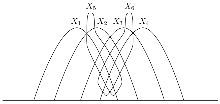
As discussed in Section 5, the -Measure of a finite-length Markov chain can be represented by a 2-dimensional information diagram as in Fig. 9. Such an information diagram is a “correct” representation in the sense that the closed curves representing the set variables intersect with each other in such a way that
-
1.
all the Type I atoms are nonempty (not suppressed);
-
2.
all the Type II atoms are empty (suppressed).
We call Fig. 9 an information diagram (customized) for a Markov chain, or more specifically an information diagram for the path (as discussed in Section 5). With such an information diagram, it is relatively easy to discover information inequalities and identities pertaining to a Markov chain by visualization, which may be difficult otherwise. A notable such example is an information identity for a Markov chain of five random variables that was useful in proving an outer bound for multiple descriptions [16] (see also [18, Example 3.18]).
Owing to its simple and regular structure, it is possible to construct an information diagram for a Markov chain by trial and error. However, constructing an information diagram for a general MRF requires a more systematic approach. In the rest of this section, we develop a method for this purpose by using the characterization of a subfield of an MRF in Section 4.
To simplify notation, we use to denote . Consider forming a Markov graph with . Using Corollary 3 as the recipe, we can construct . Then by repeating this step with in place of , we can construct , which from Proposition 6 is in fact equal to . In the same fashion, we can construct the graphs recursively.
In our method for constructing an information diagram for , we construct a sequence of information diagrams for , recursively, with the last one being the desired information diagram. Denote these information diagrams by . For the convenience of discussion, denote the closed curve representing by for .
Now the graph consists of the single vertex 1 and no edge. Then an information diagram consisting of any closed curve representing would be a correct representation for . Call this information diagram .
We observe that for , an atom generates the two atoms and in , and there is the extra atom in that is not generated by any atom in .
For , in constructing from , we add the closed curve to the former in a suitable way. In order for this recursive approach to work, we need to ensure that a Type II atom of that is suppressed in would not generate a Type I atom of which is not to be suppressed in . This is proved in the next theorem.
Theorem 16.
For , if is a Type II atom of , then both and are Type II atoms of .
Proof Assume that is a Type II atom of . We first prove that is a Type II atom of . From the discussion following Proposition 6, we know that is a subgraph of . As such, upon removing all the vertices in in both graphs, we see that is subgraph of , where the latter is disconnected because is a Type II atom of . It then follows that is also disconnected. Upon noting that , we see that which is disconnected. Therefore, is a Type II atom of .
We now prove that is a Type II atom of . Let
| (21) |
be the set of neighbors of vertex in . Note that . Let and be the sets of edges of and , respectively. Evidently,
| (22) |
where is the set of neighbors of vertex in . We consider two cases for .
This is the case when vertex has no neighbor in . Since is a Type II atom of , is disconnected. From (22), we have , so that . This implies that is also disconnected. Upon noting that , we have which is disconnected. Therefore, is a Type II atom of .
This is the case when vertex has at least one neighbor in . For any distinct vertices and that are both neighbors of vertex in (and therefore also neighbors of vertex in ), according to Corollary 3, is an edge in and hence (because ), which implies that and belong to the same component in . Equivalently, if and belong to different components in , then and cannot both be neighbors of in . Therefore, the neighbors of in all belong to the same component in , and we denote this component by .
Since is disconnected, there exists another component in . Now consider any and . Since and are in different components in , we have . Then we see from the discussion in the last paragraph that and cannot both be neighbors of in . By Corollary 3, is not an edge in and hence not an edge in because is a subgraph of . Therefore, . Also, since all the neighbors of vertex in are in , is not a neighbor of vertex in , and therefore .
Summarizing the above, we have proved that for any and , . Hence, and are distinct components in , so that is disconnected. Finally, upon noting that , we see that is a Type II atom of .
When we construct by adding to , for each Type I atom of , the closed curve is required to
-
(B1)
Split into two regions if both and are Type I atoms of , so that both and are not suppressed in ;
-
(B2)
Include in if and are Type I and Type II atoms of , respectively, so that is not suppressed and is suppressed in ; or
-
(B3)
Exclude from if and are Type II and Type I atoms of , respectively, so that is suppressed and is not suppressed in .
However, if both and are Type II atoms of , there is no way the closed curve can be drawn such that both of these atoms are suppressed in . Under this situation, our recursive approach for constructing an information diagram for would not work. The following theorem (see Corollary 5) precludes this possibility.
Theorem 17.
If is a Type I atom of , then
-
i)
if , then A belongs to (B3);
-
ii)
if , then A belongs to (B1);
-
iii)
if , then A belongs to either (B1) or (B2).
Corollary 5.
If is a Type I atom of , then at least one of and is a Type I atom of .
Proof of Theorem 17 Let and be the edge sets of and , respectively. By Corollary 3, we have
| (23) |
which implies
| (24) |
Let and be the edge sets of and , respectively. We see that and can be obtained respectively from and by removing the edges joining at least one vertex in from these sets. Then upon removing these edges from every set in (24), we obtain
| (25) |
Assume is a Type I atom of . We now prove the theorem for each of the three cases.
i)
We first prove that is a Type I atom of . Since , i.e., , it follows from (25) that , or . In fact,
| (26) |
because in general (cf. (23)). Now, if is a Type I atom of , then is connected. In view of (26), we see that is also connected. Therefore, is a Type I atom of .
We now prove that is a Type II atom of . From the last paragraph, is connected. Then all the vertices in are connected in , and they remain connected in because is a subgraph of . On the other hand, since , is not an edge in for all , and so in in , vertex is not connected with any vertex in . Since is a subgraph of , we see that in , vertex is not connected with any vertex in . Thus is disconnected. Hence, we conclude that is disconnected, i.e. is a Type II atom of .
ii)
To prove that is a Type I atom of , we only have to observe that in (25), when . Then (26) holds and we can apply the same argument as in case i).
We now prove that is a Type I atom of . For the economy of presentation, we will give a proof that also covers case iii), i.e., .
It follows from (25) that for , if and , then , i.e., . Equivalently, if or , then or . In other words, if and are not both in and , then .
Since is a Type I atom of , is connected. Then for any distinct , there exists a path between vertices and in .
If such a path does not contain an edge with both endpoints in , from the discussion in the second last paragraph, we see that all the edges on the path are in and hence are also in because is a subgraph of . In other words, and are connected in .
If the path contains any edge with both endpoints in , we can construct another path between and in by replacing every such an edge by edges and which are both in . Then we see that and are connected in .
Finally, since , there exists a vertex . Then for any , we can readily see that vertices and are connected in because is connected with and is connected with . Summarizing the above, for any distinct , and are connected in . This implies that is connected, i.e., is a Type I atom of .
ii)
To prove that belongs to either (B1) or (B2), we only need to prove that is a Type I atom of . This has already been proved in case ii).
Now in light of Theorem 16 and Corollary 5, we can construct from according to the prescriptions in (B1)-(B3) for each Type I atom of . Theorem 17 helps simplify the checking of which of (B1) to (B3) these atoms belong to, as we now explain. The three conditions for in Theorem 17 are
-
i)
: This means that for any , or equivalently, . In this case, the closed curve excludes the atom .
-
ii)
: This means that for only one . In this case, the closed curve splits the atom .
-
iii)
: This means that for more than one . If belongs to (B1), the closed curve splits the atom , otherwise ( belongs to (B2)) it includes the atom .
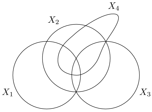
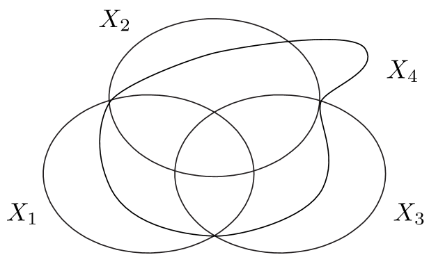
Note that if satisfies condition iii), we still need to check whether it belongs to (B1) or (B2), which is unavoidable. This is explained by the two examples in Figs. 12 and 13. In each of these examples, we have and . Consider the Type I atom of . Then and , i.e., satisfies condition iii).
Example 16.
We apply our method to construct an information diagram for the Markov chain . From Corollary 2, we see that for , is the path defined in Section 5.
The information diagram , which consists of only the set variable , is completely trivial. For , when we construct from , since (cf. (21)) is a singleton, every Type I atom in satisfies the condition that for only one . Then based on the discussion in the foregoing, the closed curve excludes every Type I atom in that is not contained in and splits every Type I atom in that is contained in . This way, we can obtain the information diagram in Fig. 9.
Our method is robust in the sense that it works for any labeling of the vertices. However, it may be more convenient to construct the information diagram for one labeling than another. This is illustrated in the following two examples.
Example 17.
Example 18.
Consider the graph in Fig. 10, which is the same as the one in Fig. 14 except that the vertices are labelled differently. Here, is the complete graph , and so there is no Type II atom in . Now . We have to consider all the atoms that are subsets of , namely all the atoms in because . For the atoms , , and in , since each of them is a subset of for only one , the closed curve splits each of these atoms. For an atom equal to , , or , we can check that and . Therefore, belongs to (B2). For the atom , we can check that and , so this atom also belongs to (B2). As such, the closed curve includes all these four atoms, and we can construct the information diagram in Fig. 16. It can readily to checked that this information diagram is equivalent to the one in Fig. 15 constructed in Example 17.
Example 19.
Figs. 17 and 18 show a graph and the corresponding information diagram, respectively. In light of Corollary 2, we see that is the path defined in Section 5. Then we can use the information diagram for as and add to it the closed curves and using the technique in Example 16 to obtain the information diagram in Fig. 18.
7 Conclusion
The theory of -Measure proves to be a very useful tool for characterizing full conditional independence structures and MRFs [15], because with the -Measure, the fundamental set-theoretic structure of the problem is revealed. In this paper, we apply this tool to obtain three main results related to MRFs.
For an MRF represented by an undirected graph, a subfield is a subset of the random variables forming the MRF . We have determined the smallest undirected graph that can always represent a subfield as an MRF. This is our first main result. As an application of this result, we have obtained a necessary and sufficient condition for a subfield of a Markov tree to be also a Markov tree.
A Markov chain can be regarded a special case of an MRF. It was previously known that the -Measure of a Markov chain is always nonnegative [11]. Here, we have proved that the -Measure is nonnegative for every MRF represented by a given undirected graph if and only if the graph is a forest of paths, i.e., the Markov random field is a collection of independent Markov chains. This means that Markov chains are essentially the only MRFs such that the -Measure is always nonnegative. This is our second main result. In the course of proving this result, we have obtained some interesting properties of the -Measure pertaining to an MRF.
Our third main result is a nontrivial application of our first main result. In [11], a construction of an information diagram for a Markov chain was presented. By applying our first main result, we have developed a recursive approach for constructing information diagrams for MRFs. Such diagrams not only reveal the special structure of the -Measure for an MRF, but they also are very useful for identifying information identities and inequalities pertaining to an MRF.
The work in our paper is based upon the the view that an MRF is a collection of full conditional mutual independencies. As such, some of our results can potentially be generalized for Markov structures beyond MRFs.
Appendix A Proof of Proposition 6
Let
and
Consider any . By the definition of , there exists a path between and in on which all the intermediate vertices are in . Now on this path, let be the vertices in in the direction from to . Then the vertices between and , the vertices between and for , and the vertices between and are all in , because . By the definition of , the edges , for , and are in . In other words, there is a path between and in on which all the intermediate vertices are in . Then by the definition of , . This proves that .
On the other hand, consider any . By the definition of , there exists a path between and in on which all the intermediate vertices are in . Let the edges on this path be , , , , and , where are in . Since , by the definition of , there exists a path between and on which all the intermediate nodes are in . Similarly, there exists a path between and for , and a path between and , on which all the intermediate nodes are in . Thus there exists a path between and in on which all the intermediate nodes are in , because . Then by the definition of , . This proves that .
Hence, we conclude that , i.e., . The proposition is proved.
Appendix B Verification of in the Proof of Theorem 14
In this appendix, we verify that as prescribed by (20) satisfies (19). First, for , consider
From (20), we see that in the above summation vanishes if , and so
| (27) | |||||
This verifies (19) for the case . Next, for , consider
| (28) | |||||
It follows from (27) and (28) that
| (29) | |||||
| (30) | |||||
| (31) |
This verifies (19) for the case . Now for , consider
In the above, since , we see from (20) that every term in the above summation vanishes, and so
| (32) |
Finally, consider such that and let be two arbitrary elements of . Then in light of (31) and (32), we have
where the inequality above is justified by the union bound because is nonnegative on all the atoms in (cf. (20)). On the other hand, we have
again because is nonnegative on all the atoms in . Therefore, , verifying (19) for the case .
Appendix C Proof of Lemmas 4 and 5
Lemma 6.
Let be a connected undirected graph and . Then
-
a)
for any , we have for all , where () are the components of ;
-
b)
for all nonempty subset of .
Proof We assume that , since otherwise and the lemma has no assertion.
We first prove a). Let , and by the definition of , we have . Consider any spanning tree of . Note that must contain at least one edge connecting and each () because is connected. For any fixed , consider such an edge and call it . Upon removing , is disconnected with one component being a subtree containing and the other component being a subtree not containing . For the latter subtree, all the vertices are in , otherwise there exists an edge connecting and (), which is a contradiction because are the components of . Then this subtree must have at least one leaf in , say . Note that is not a cutset in and hence not a cutset in . Therefore , proving a).
We now prove b). Consider any nonempty subset of and fix . Since , we have . By a), for all , with . Then the vertices in are not all connected in , and hence not all connected in because and . This implies that is not connected, or . The lemma is proved.
Lemmas 4 and 5 can now be obtained as follows. In Theorem 11, is a Type I atom, and so is connected. The same holds for Lemmas 4 and 5. Lemma 4 is trivial for . For , it can be obtained by applying Part a) of Lemma 6 to . Finally, by applying Part b) of Lemma 6 to with , we obtain Lemma 5.
Acknowledgment
The authors would like to thank Prof. Leizheng Cai, and Prof. František Matúš for the useful discussions.
References
- [1] Hu Guo Ding, “On the amount of information,” Teor. Veroyatnost. i Primenen., 4: 447-455, 1962 (in Russian).
- [2] J. M. Hammersley and P. Clifford, “Markov fields on finite graphs and lattices,” (unpublished) 1971.
- [3] F. Spitzer, “Random fields and interacting particle systems,” M.A.A. Summer Seminar Notes, 1971.
- [4] J. Moussouris, “Gibbs and Markov random systems with constraints,” J. Stat. Physics, vol. 10, pp. 11-33, 1974.
- [5] C. Preston, Random Fields, Springer-Verlag, 1974.
- [6] R. Kindermann and J. L. Snell, Markov Random Fields and their Applications, American Mathematical Society, 1980.
- [7] S. Asmussen and D. Edwards, “Collapsibility and response variables in contingency tables,” Biometrika, vol. 70, no. 3, pp. 567-578, Dec 1983.
- [8] J. Pearl and A. Paz, “GRAPHOIDS: A graph-based logic for reasoning about relevance relations,” Technical Report 850038 (R-53-L), Cognitive Systems Laboratory, University of California, Los Angeles, 1985. Short version in Advances in Artificial Intelligence – II, ed. B. Du Boulay, D. Hogg, and L. Steels, pp. 357-363, Amsterdam: North Holland, 1987.
- [9] R. W. Yeung, “A new outlook on Shannon’s information measures,” IEEE Trans. Inform. Theory, vol. 37, pp. 466-474, May 1991.
- [10] F. M. Malvestuto, “A unique formal system for binary decompositions of database relations, probability distributions, and graphs,” Information Sciences 59 (1992) 21-52; with Comment by F. M. Malvestuto and M. Studený, Information Sciences 63 (1992), 1-2.
- [11] T. Kawabata and R. W. Yeung, “The structure of the -Measure of a Markov chain,” IEEE Transactions on Information Theory, vol. 38, pp. 1146-1149, May 1992.
- [12] D. Geiger and J. Pearl, “Logical and algorithmic properties of conditional in- dependence and graphical models,” Annals of Statistics, vol. 21, no. 4, pp. 2001-2021, 1993.
- [13] S. L. Lauritzen, Graphical Models, Oxford Science Publications, Oxford, 1996.
- [14] R. W. Yeung, “A framework for linear information inequalities,” IEEE Trans. Inform. Theory, vol. 43, pp. 1924-1934, Nov 1997.
- [15] R. W. Yeung, T. T. Lee, and Z. Ye, “Information-theoretic characterizations of conditional mutual independence and Markov random fields,” IEEE Trans. Inform. Theory, vol. 48, pp. 1996-2011, Jul 2002.
- [16] F. Fu and R. W. Yeung, ”On the rate-distortion region for multiple descriptions,” IEEE Trans. Inform. Theory, vol. 48, pp. 2012-2021, Jul 2002.
- [17] L. E. Doyle, A. C. Kokaram, S. J. Doyle, and T. K. Forde, “Ad hoc networking, Markov random fields, and decision making,” IEEE Signal Processing Magazine, vol. 23, no. 5, pp. 63-73, Sept 2006.
- [18] R. W. Yeung, Information Theory and Network Coding, Springer, 2008.
- [19] S.-e. Jeon and C. Ji, “Randomized and distributed self-configuration of wireless networks: Two-layer Markov random fields and near-optimality,” IEEE Trans. Signal Processing, vol. 58, no. 9, pp. 4859-4870, Sept 2010.
- [20] Y. O. Yazir, R. Farahbod, A. Guitouni, S. Ganti, and Y. Coady, “Adaptive routing in mobile ad hoc networks based on decision aid approach,” 8th ACM International Workshop on Mobility Management and Wireless Access, Bodrum, Turkey, Oct 17-18, 2010.
- [21] A. Blake, P. Kohli, and C. Rother (Ed.), Markov Random Fields for Vision and Image Processing, MIT Press, 2011.
- [22] T. A. B. Snijders, “Statistical models for social networks,” Annual Review of Sociology, vol. 37, pp. 131-153, 2011.
- [23] T. Wang, H. Krim, and Y. Viniotis, “A generalized Markov graph model: Application to social network analysis,” IEEE J. Selected Topics in Signal Processing, vol. 7, pp. 318-332, 2013.
- [24] A. Sandryhaila and J. M. F. Moura, “Big data analysis with signal processing on graphs: Representation and processing of massive data sets with irregular structure,” IEEE Signal Processing Magazine, vol. 31, pp. 80-90, 2014.
- [25] M. Studený, Probabilistic Conditional Independence Structures, Springer-Verlag 2005.
- [26] K. Sadeghi, “Stable mixed graphs,” Bernoulli 19, pp. 2330-2358, 2013.
- [27] K. Sadeghi, “Marginalization and conditioning for LWF chain graphs,” Annals of Statistics, vol. 44, no. 4, pp. 1792-1816, 2016.
