11email: {sungjoon.choi, kyungjae.lee, songhwai.oh}@cpslab.snu.ac.kr 22institutetext: Rethink Robotics, Boston, MA, USA
22email: apark@rethinkrobotics.com
Density Matching Reward Learning
Abstract
In this paper, we focus on the problem of inferring the underlying reward function of an expert given demonstrations, which is often referred to as inverse reinforcement learning (IRL). In particular, we propose a model-free density-based IRL algorithm, named density matching reward learning (DMRL), which does not require model dynamics. The performance of DMRL is analyzed theoretically and the sample complexity is derived. Furthermore, the proposed DMRL is extended to handle nonlinear IRL problems by assuming that the reward function is in the reproducing kernel Hilbert space (RKHS) and kernel DMRL (KDMRL) is proposed. The parameters for KDMRL can be computed analytically, which greatly reduces the computation time. The performance of KDMRL is extensively evaluated in two sets of experiments: grid world and track driving experiments. In grid world experiments, the proposed KDMRL method is compared with both model-based and model-free IRL methods and shows superior performance on a nonlinear reward setting and competitive performance on a linear reward setting in terms of expected value differences. Then we move on to more realistic experiments of learning different driving styles for autonomous navigation in complex and dynamic tracks using KDMRL and receding horizon control.
Keywords:
Model-free, inverse reinforcement learning, autonomous driving1 Introduction
Modern autonomous robots are expected to operate complex and complicated tasks such as autonomously driving in dynamic urban streets [12] or providing personalized services to clients [15]. As an explicit rule-based programming has weakness in handling diverse and exceptional uncommon cases, reinforcement learning (RL) has received a great deal of attention [16]. When applying RL to practical real-world problems, designing an appropriate reward function is the most important part as it directly affects the quality of the resulting policy function.
When it comes to problems for which explicitly designing a reward function is challenging, RL might not be an opportune choice to select. For example, manually describing a proper reward function that can generate socially acceptable driving behavior styles [12] or acrobatic fight of a helicopter [1] can be cumbersome. On the contrary, as humans can easily demonstrate such behaviors, it is more effective to first collect demonstrations of an expert and let robots mimic the expert. This problem of imitating human-controlled behaviors is often referred to as imitation learning [25].
Imitation learning can be categorized into two groups based on which function we are inferring about [25]. The first group focuses on directly mimicking the policy function which maps the state space or observations to the set of possible actions. The other group focuses on reconstructing the underlying reward function, which is a succinct representation of an expert’s objective [19]. This approach is often referred to as inverse optimal control [17] or inverse reinforcement learning (IRL) [19]. While it is often more difficult to infer the underlying reward function, IRL has a clear advantage over direct policy learning in terms of generalization performance and transferability. In other words, the trained reward function can further be used to obtain optimal control in unseen situations (generalization) or even to different model dynamics (transferability). However, most of the IRL methods require discretization of the state space and full specification of the model dynamics as it solves a Markov decision problem as a subroutine. This obstructs model-based IRL methods to be applied to large scale systems with continuous state and action spaces. To overcome this issue, few model-free IRL methods have been proposed recently. However, these methods are often based on sampling to compute the reward function, which takes a fair amount of time.
In this paper, we propose a density based model-free inverse reinforcement learning algorithm, named density matching reward learning (DMRL). DMRL first computes the empirical distribution of expert’s trajectories and finds a reward function that maximizes the inner-product between the empirical distribution and the reward function. In other words, we optimize the reward function that best matches the empirical state-action distribution of an expert [14]. Furthermore, we perform theoretical analyses of the proposed method and derived the sample complexity of the proposed method under mild assumptions. To handle nonlinear reward functions, kernel DMRL (KDMRL) is also proposed. KDMRL has been applied to two experiments: grid world and track driving experiments. In grid world experiments, KDMRL shows superior performance for cases with nonlinear reward functions and comparable performance to linear IRL methods for linear reward functions in terms of expected value differences. In track driving experiments, KDMRL outperforms all other compared methods in terms of mimicking experts’ driving style as well as safety and stability of driving.
2 Related Work
Recently proposed inverse reinforcement learning (IRL) methods can be grouped by two different criteria. The first criterion is about how we define the objective function of the IRL problem: margin based or probabilistic model based methods. On the other hand, the second criterion is about the necessity of the transition model, i.e., , of the underlying Markov decision process. The classification of state-of-the-art IRL algorithms, including ours, is summarized in Table 1.
| Model-based | Model-free | |
|---|---|---|
| Margin based model | [2, 23, 24] | [9] |
| Probabilistic model | [29, 8, 18, 27, 26] | [4, 10, 13], Ours |
A margin based approach aims to maximize the margin between the value of the expert’s policy compared to other possible policies. An IRL problem was first introduced by Ng and Russell [19], where the parameters of the reward function are optimized by maximizing the margin between randomly sampled reward functions. Abbeel and Ng [2] proposed an apprenticeship learning algorithm, which minimizes the difference between the empirical distribution of an expert and the distribution induced by the reward function. Ratliff et al. [23] proposed the maximum margin planning (MMP) algorithm, where Bellman-flow constraints are utilized to maximize the margin between the experts’ policy and all other policies.
On the other hand, probabilistic model based methods aim to find the reward function which maximizes the likelihood or posterior distribution. Zeibart et al. [29] proposed maximum entropy IRL (MaxEnt) using the principle of maximum entropy to alleviate the inherent ambiguity problem of the reward function. In [22], Ramachandran et al. proposed Bayesian IRL (BIRL), where the Bayesian probabilistic model was defined and effectively solved by using a Metropolis-Hastings sampling method. Levine and Koltun [18] proposed Gaussian process inverse reinforcement learning (GPIRL), where a nonlinear reward function is effectively modeled by a sparse Gaussian process with inducing inputs.
Recently, several model-free IRL methods have been proposed. In [4], Boularias et al. proposed a relative entropy IRL (RelEnt) method, which minimizes the relative entropy between the empirical distribution of demonstrations from the baseline policy and the distribution under the learned policy. Structured classification based IRL [9] was proposed by formulating IRL problem as a structured multi-class classification problem by founding that the parameters of the action-value function are shared with those of the reward function. In [13], Herman et al. proposed a model-free IRL method by simultaneously estimating the reward and dynamics, where they separate the real transition model (dynamics) and the belief transition model of an agent to handle previously unseen states. Finn et al. [10] proposed a guided cost learning, which extends the maximum entropy IRL to a model-free setting based on approximation by importance sampling. In this paper, we propose a model-free IRL method that first compute the empirical state action distribution of an expert and then find the reward function that matches the density function.
3 Problem Formulation
Before presenting the proposed inverse reinforcement learning (IRL) method, let us introduce the objective of reinforcement learning (RL). In particular, we will consider an average reward RL problem, which often has advantages over discounted formulations with respect to stabilities as we do not have to choose a discount factor or time horizon [16]. An average reward RL problem can be formulated as follows:
| (1) | ||||||
| subject to | ||||||
where is a conditional distribution of action given state , i.e., , and is a stationary state distribution induced by policy . Using a chain rule, we can easily define a joint state-action distribution and rewrite the RL formulation in (1) as follows:
| (2) | ||||||
| subject to |
where indicates an inner-product operation and is a feasible set of induced by the model dynamics which is often referred to as a Bellman flow constraint. Intuitively speaking, the objective of RL in (2) is to find a stationary state-action distribution given a reward function considering a Bellman flow constraint , where the policy function can naturally be derived from as [16].
As the objective of IRL is to recover given a set of trajectories , where a single trajectory consists of state-action pairs, , existing IRL methods either try to maximize a margin between values of expert’s trajectories and other sampled or every possible values [19, 2, 23] or estimate the parameters of a reward function by properly defining the likelihood (probability density) of trajectories [29, 18, 22, 4, 27].
In this paper, we cast the reward estimation problem as a density matching problem. In particular, we first assume that the demonstrations are sampled from the stationary state-action distribution and estimate the probability density of the state-action space using a set of expert’s trajectories . In this paper, kernel density estimation with radial basis functions [28] is used to estimate the joint state-action density as , but other suitable estimator can be applied. Then, the underlying reward function is estimated from the following optimization problem, which we call density matching reward learning (DMRL):
| (3) | ||||||
| subject to |
where the norm ball constraint is introduced to handle the scale ambiguity of the reward function [19] and .
Suppose that we have access to the true stationary state-action density and estimate the reward from (3), i.e., . We define the value of with respect to the true state-action density as an optimal value . In other words, the optimal value is an expectation of reward with respect to the true state-action density , i.e.,
| (4) |
Similarly, we define an estimated value as an expectation of an estimated reward computed from solving (3) with estimated density with respect to the true state action density , i.e.,
| (5) |
Of course, estimating the true density is practically infeasible as it requires an infinite number of samples. In Section 4, we give a probabilistic bound on the absolute difference between and , i.e., as a function of the number of trajectories (sample complexity). Furthermore, the proposed method can be easily extended to a continuous domain using the kernel method [21] as described in Section 5.
4 Theoretical Analysis
In this section, we present a bound on the sample complexity of the proposed method, DMRL. In particular, we will focus on the absolute difference between the optimal value and estimated value , i.e., . We would like to note that this analysis is not based on the expected value difference (EVD), which is used in [2, 9] to theoretically analyze the performance of IRL methods. This is mainly because only reward functions linear with respect to parameters can be analyzed using EVDs. We instead show the sample complexity on the absolute difference between the best value and the optimized value, , with samples. As , minimizing this quantity can be interpreted as minimizing the difference between the estimated reward and the true reward when projected by the true state-action density .
Followings are the main results of this paper.
Theorem 4.1
Let be computed from and be computed from , where and are estimated and true densities, respectively. Then
where is the variational distance111 The variational distance between two probability distributions, and , is defined as . It is also known that . between two probability distributions.
Theorem 4.2
The main intuition behind the proposed DMRL is that IRL can be viewed as a dual problem of finding a reward function that matches the state-action distribution [14]. The domain of our interest is the product space of states and actions, , and for the notational simplicity, we will denote this space as . Before proving Theorem 4.1 and 4.2, let us first introduce useful lemmas.
Lemma 1
[11] Let and be probability distributions over and be a bounded function on . Then,
Lemma 2
[20] Suppose and are probability distributions. Then,
where is the Hellinger distance222 The Hellinger distance between two probability distributions and is defined as .
Lemma 3
[3] Suppose is a proper norm defined on index set . Then, for any ,
Theorem 4.3
Suppose Assumption 1–8 in Appendix A hold. Let and be the number of samples and basis functions for kernel density esimation, respectively, and be the estimated density function from kernel density estimation with samples and basis functions. Then, for any and and sufficiently large, we have
where is a squared Hellinger distance between two probability distributions.
Proof (Theorem 4.1)
Let and be the true and estimated density functions, respectively, and and be the reward functions estimated by DMRL with and , respectively. The absolute difference between the optimal value and the estimated value can be expressed as:
where we used the triangular inequality and Lemma 1.
can be further bounded by
where we used the definition of optimal and estimated values, Lemma 3 for a dual norm, the definition of an inner product, and the definition of .
5 Kernel DMRL
The proposed DMRL method can be extended to a continuous state-action space using a kernel-based function approximation method, which will be referred to as kernel density matching reward learning (KDMRL). In particular, we assume that the reward function is in the reproducing kernel Hilbert space (RKHS) with a finite set of inducing inputs. The original DMRL formulation in (3) can be relaxed by solving the following optimization problem:
| (7) |
where is the estimated density function, controls the smoothness of the reward function, is a set of inducing points, and is the squared Hilbert norm, which is often used as a regularizer for kernel machines. Then, the reward function with inducing inputs can be expressed as
| (8) |
where is a state-action pair, is a set of pre-defined inducing points, is a parameter determining the shape of the reward function, and is a positive semidefinite kernel function. In other words, optimizing in (7) is equivalent to optimizing dimensional vector and the squared Hilbert norm of , where and is a kernel matrix computed from .
We use kernel density estimation (KDE) to estimate the probability density function
| (9) |
where is the number of training samples, is the th training data, and is a kernel function whose integral is one (basis density function). Then, (7) can be reformulated as:
| (10) | ||||||
which can be easily solved by quadratic programming.
The objective of the kernel density estimation in (9) is to estimate the stationary distribution of an MDP. If we have infinite length trajectories, converges to the true regardless of the initial state distribution by the Ergodic theorem [11]333 Here, we assume that the state transition probability induced by the expert’s policy is ergodic.. However, as we have finite length trajectories, we have to compensate the effect of the initial distribution. In Markov chain Monte Carlo (MCMC), some initial samples known as burn-in samples are ignored when estimates are computed. However, in our case, as the length of a demonstration is not long enough to reserve burn-in samples, we differentiate the influence of each sample by giving more weights to the latter ones. In this regards, we modify the density function (9) using a leveraged kernel function proposed in [6]
| (11) |
where indicates the leverage (or influence) of the th training data, is a constant, and are the length and time-step of the trajectory, and is a normalization constant. We can rewrite (10) with an additional two norm regularization, , in a matrix form as follows:
| (12) |
where , , and are regularization coefficients, and is a vector of ’s. As (12) is quadratic with respect to the optimization variable , (12) has an analytic solution:
| (13) |
In following experiments, we use a widely used squared exponential kernel function for both and . While it is possible to optimize the hyperparameters of the kernel function by maximizing (12), we use a simple median trick [7] for determining the hyperparameters.
6 Experiments
To validate the performance of the proposed KDMRL method, two different scenarios have been investigated: grid world and track driving experiments. The grid world experiments are conducted for quantitatively comparing the performance of KDMRL against four different inverse reinforcement learning methods, maximum margin planning (MMP) [23], relative entropy inverse reinforcement learning (RelEnt) [4], maximum entropy inverse reinforcement learning (MaxEnt) [29], and Gaussian process inverse reinforcement learning (GPIRL) [18]. In the track driving experiments, we first collect three different types of driving styles by manually controlling a car in a simulated environment inspired by [17]. From the collected demonstrations, an underlying reward function is inferred and used to control the car with receding horizon control (RHC). In this case, MaxEnt, RelEnt, and GPIRL have been compared with KDMRL.
6.1 Grid World Experiments
In a grid world, an expert can make five actions, up, down, left, right, and staying. The underlying reward function is defined as , where is the th randomly-deployed location, is the number of peak points, and is randomly sampled from . In other words, the reward functions has randomly located concave or convex peaks.
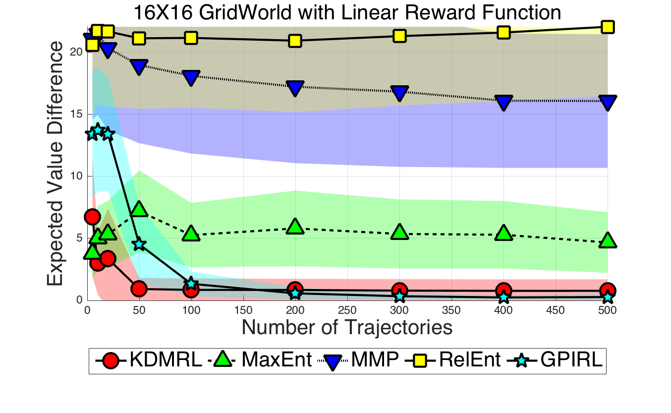
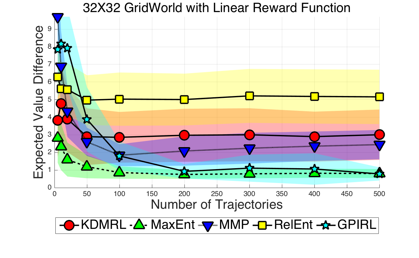
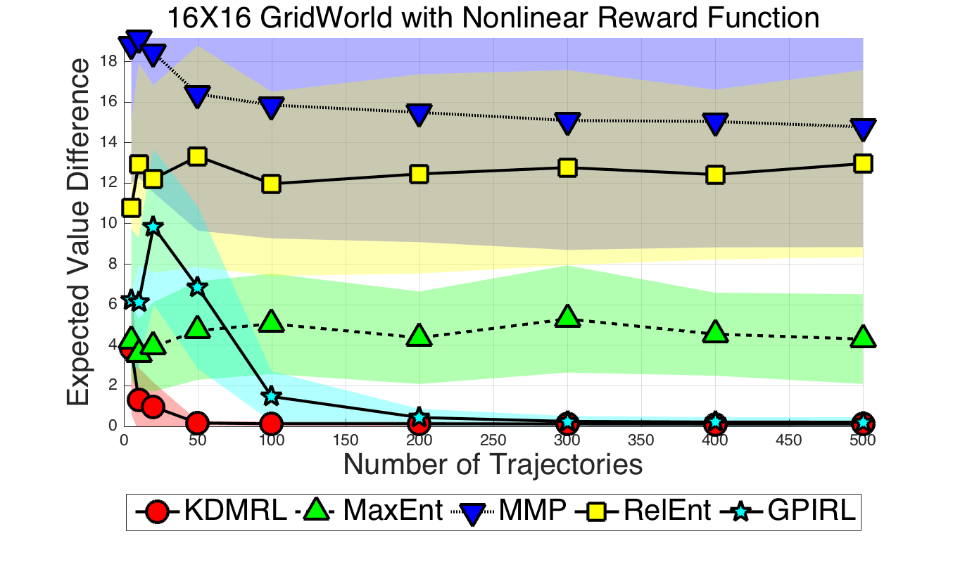
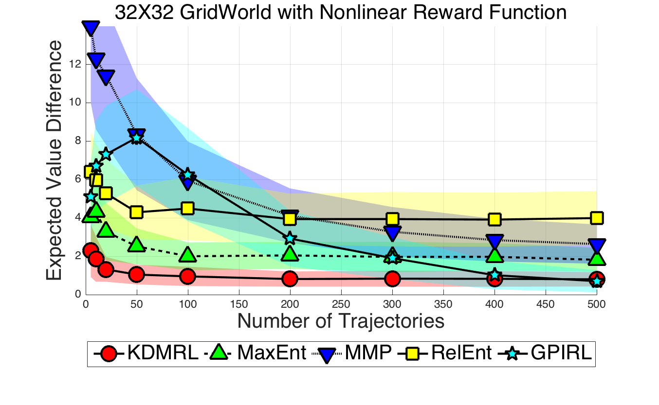
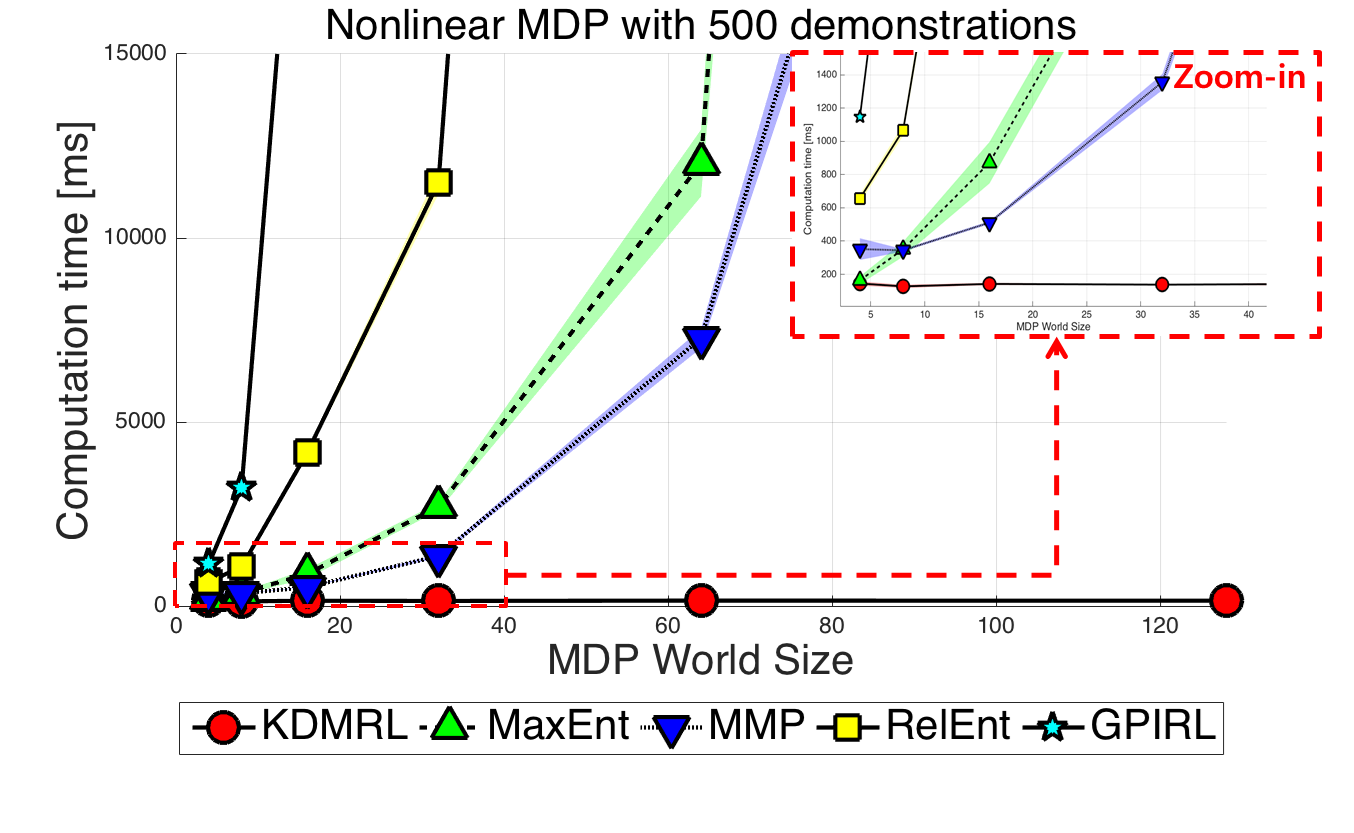
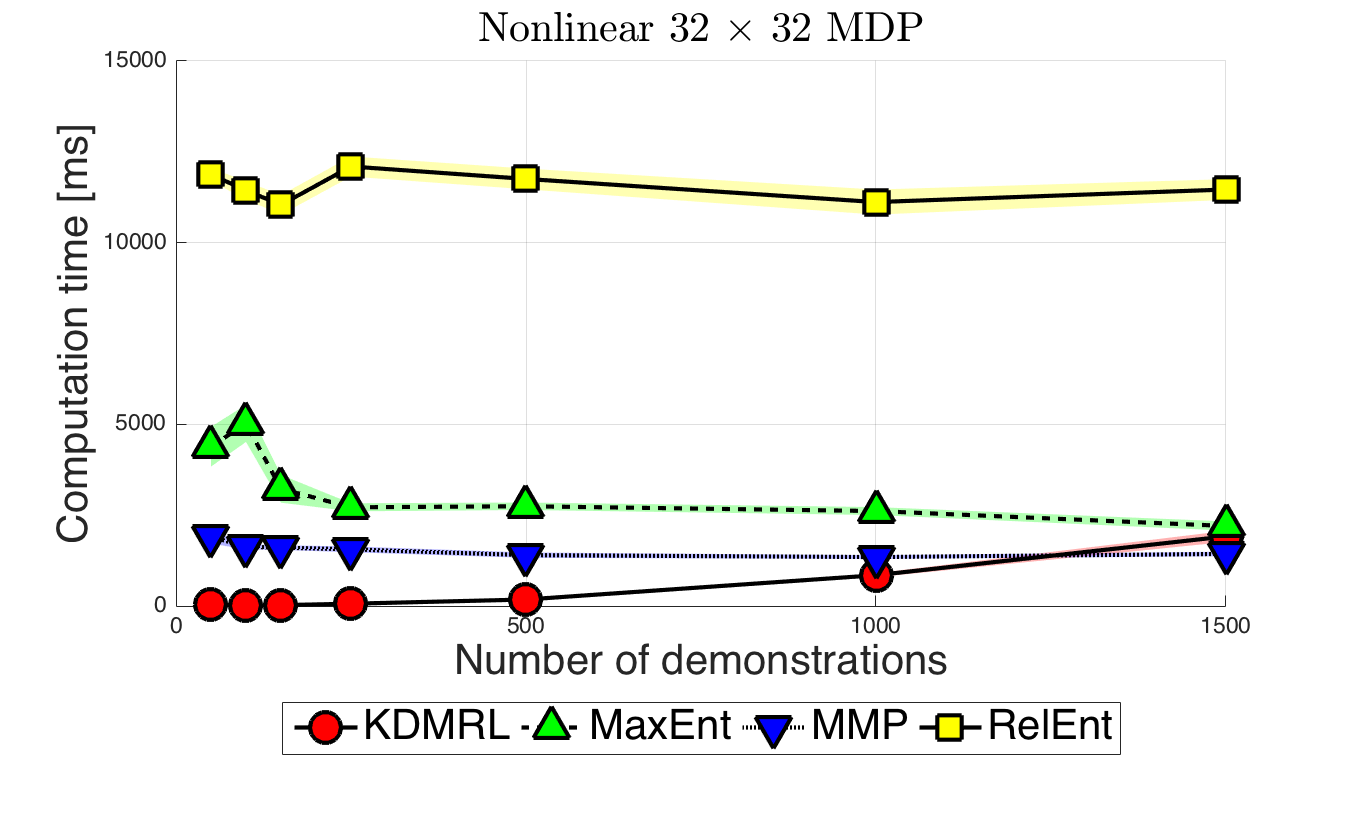
In the first set of experiments, is given as an observation or feature making the reward function as a linear function of observed features (linear reward function). In the second set of experiments, features are defined as where is equidistantly deployed points. In other words, the reward function is a nonlinear function of features (nonlinear reward function). We further separate the experiment into two grid worlds consist of and grid cells resulting four different sets of experiments. In both linear and nonlinear reward settings, we make different reward maps and collected different sets of trajectories per reward map to come up with different scenarios. The trajectories of the experts are collected by solving the underlying MDP, where lengths of trajectories are for grid world and for grid world with discount factor of . In all experiments, the number of peaks are . For KDMRL, we set for all experiments.
The expected value differences (EVDs) of IRL methods as a function of the number of trajectories are shown in Figure 1–1. In the linear reward setting, KDMRL outperforms linear-based IRL methods, MaxEnt, MMP, and RelEnt and shows performance comparable to GPIRL. However, in the linear reward setting, model-based MaxEnt and MMP show better performance compared to KDMRL. But KDMRL still outperforms RelEnt, which is the only compared model-free IRL method. We believe that this is mainly due to two reasons. The first comes from the lack of world dynamics and the second comes from the limitation of a kernel-based method as it is not appropriate for modeling a linear function (unless a linear kernel function is used). On the other hand, in the nonlinear reward cases, KDMRL outperforms all linear IRL methods. KDMRL also outperforms GPIRL for both and cases when the number of samples is less than and shows comparable performance as more samples are used.
The time complexities are shown in Figure 1–1. The computation time of KDMRL is less than ms in grid world on GHz quad core processors. While the computation time increases linearly to the number of demonstrations, it is independent from the size of the state space as it does not solve an MDP as its subroutine. This property plays a significant role in forthcoming experiments where the state space is much bigger.
6.2 Track Driving Experiments
In this experiments, we move on to more realistic and practical scenario, track driving experiments. In particular, we aim to learn three different driving styles (safe driving, speedy Gonzales, and tailgating modes) from human demonstrations, which is similar to the experiments in [17]. All three driving styles have common objective of maintaining the center of the lane while avoiding collision with other cars. However, the safe driving and speedy Gonzales modes avoid cars in front while the tailgating mode follows closely behind another car. In the safe driving and speedy Gonzales modes, a car moves at and , respectively.
The proposed method, KDMRL, is compared with MaxEnt, GPIRL, and RelEnt. MMP is not compared as it shows poor performance on nonlinear grid world experiments. In the implementation of KDMRL, we define the inducing set as a union of training inputs with randomly sampled inputs similar to [18], where the hyperparameters are selected using a simple median trick [7].444 While it is possible to fine-tune the hyperarameters as (12) is differentiable with respect to the hyperparameters, we omit this step as a simple median trick works well for this case.
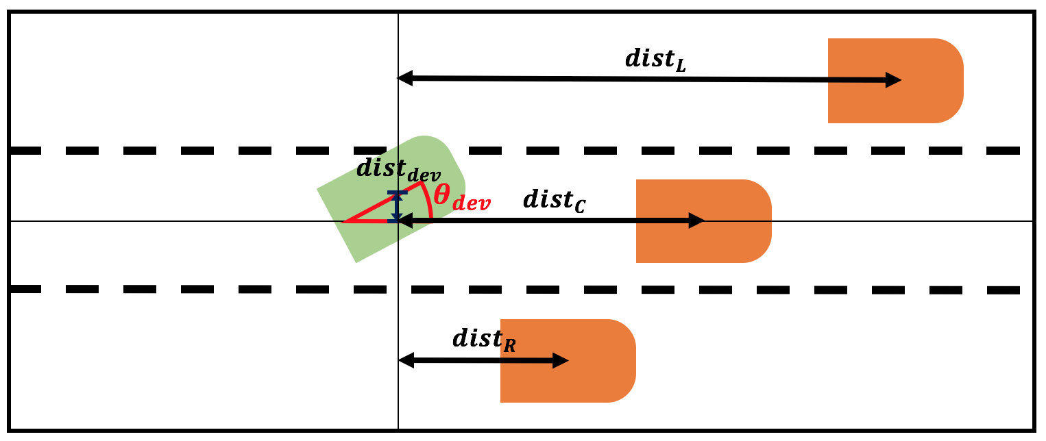
The state and action consist of the pose (, , and ) of a car following a unicycle dynamic model and directional and angular velocities (), respectively. Both state and action spaces are discretizes for model based IRL methods by dividing the state space into states, for vertical axis, for horizontal axis, and for heading, and the action space is divided into actions, for directional and for angular velocities. We used six dimensional features to represent the reward function: (1) the lane deviation distance, , (2) the lane deviation degree, , the closest frontal distances to other car in the (3) left lane, , (4) center lane, , and (5) right lane, , and (6) the directional velocity, , as depicted in Figure 2.
The demonstrations are manually collected by human demonstrators with a simple straight road configuration with three lanes and randomly deployed cars as depicted in Figure 2. For each driving mode, different settings of one to five randomly deployed car configurations are used. The demonstrations are collected by starting the car at each lane resulting episodes for each mode. Once a reward function is trained, we use a receding horizon controller to control the car.
We performed two sets of experiments to evaluate the performance of different IRL methods on track driving experiments. In the first set of experiments, the car is navigated in the road configuration where the demonstrations are collected. As we have the expert-controlled trajectories, we compute the similarity measure between the reference and resulting trajectories in terms of the variational distances. Followings are the six variational distances:
-
1.
to represent actual traversed distributions
-
2.
to check collision avoiding behaviors
-
3.
to check center maintaining behaviors
-
4.
to check center maintaining behaviors
-
5.
to check approaching behaviors for tailgating mode
-
6.
to check approaching behaviors for tailgating mode
where is a variational distance and and indicate the empirical distributions from the reference trajectories and trajectories from the RHC, respectively. The average collision ratio is also computed by averaging the number of collided trajectories among trajectories for each mode.
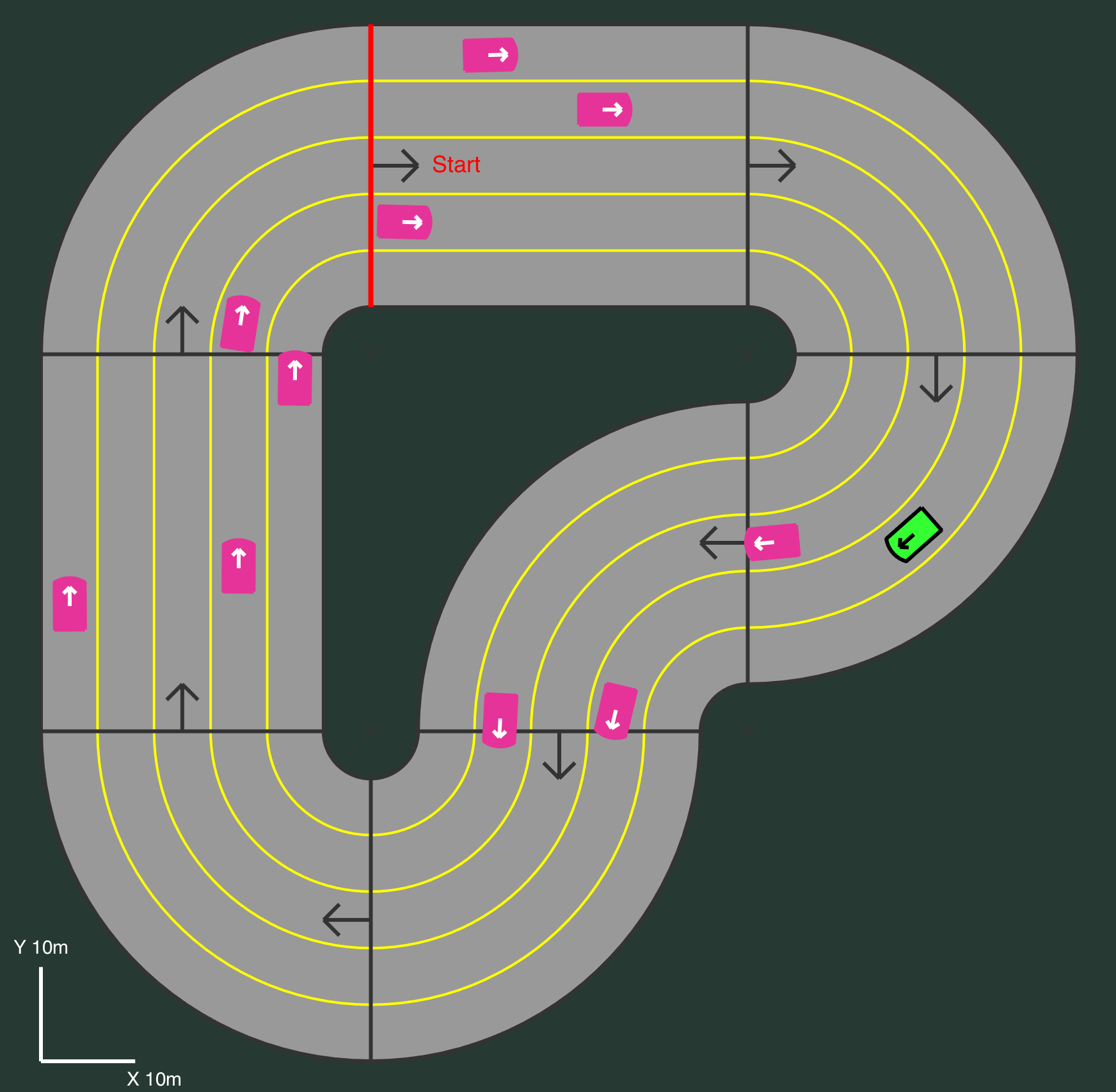
We further tested the controller on more complex and dynamic track environments with five lanes, which is depicted in Figure 2. This transfer can naturally be done as we used a feature-based representation of the reward function. Each controller navigates the track for seconds where five to ten randomly deployed cars are moving at maintaining its lane. Similar to the previous experiment, we computed the following seven measures to evaluate the performances: (1) Average number of collision, (2) Absolute average lane deviation distance, (3) Absolute average lane deviation degree, (4) Average directional velocity, and (5) Average number of lane changes.
The results of both trained and transferred scenarios are shown in Table LABEL:tbl:track_exp. (Also see the video submission for examples.) First of all, in the trained scenarios, KDMRL outperforms all other methods in terms of both collision ratio and variational distances with large margins. In particular, KDMRL navigates without any collision. GPIRL, which shows a superior performance on grid world experiments, shows second best performance on safe driving and speedy Gonzales mode. For the tailgating mode, however, it shows collision rate. It is mainly because it collides to a car in front while trying to drive behind other cars.
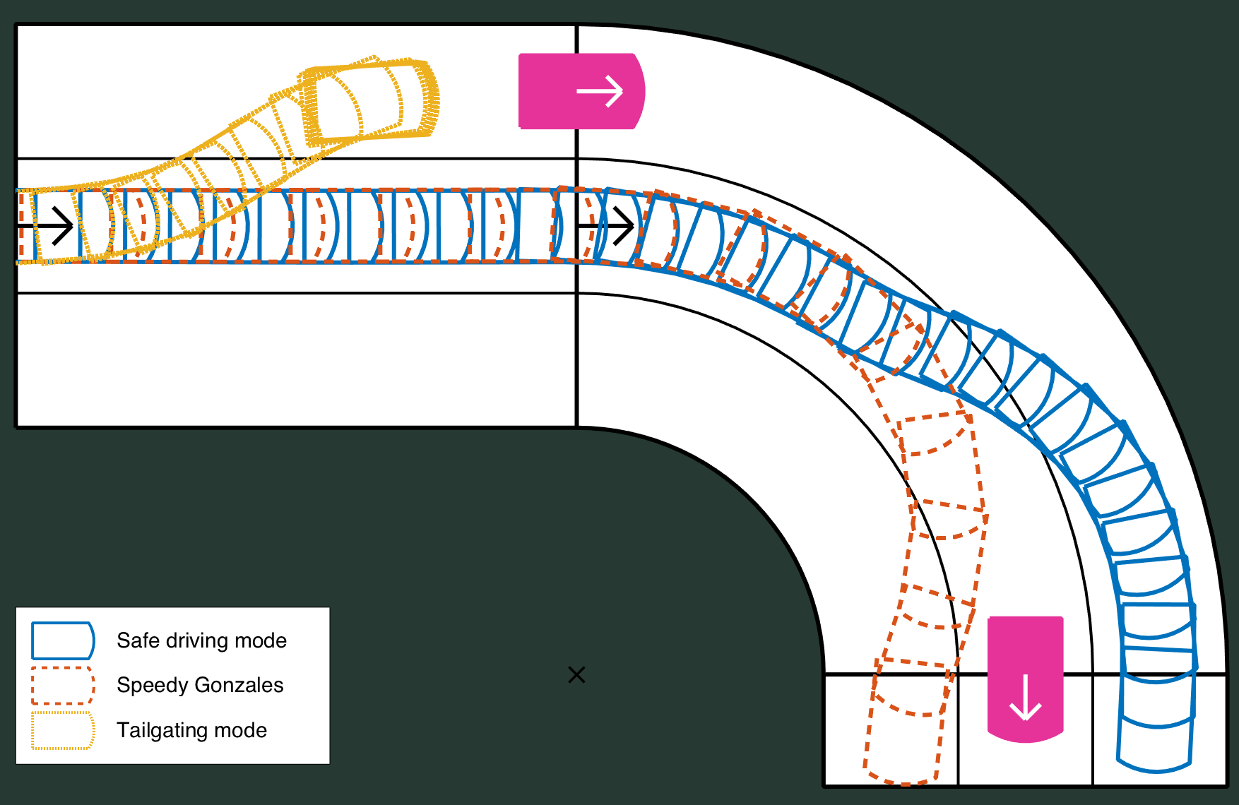
In the transferred scenarios, the absolute average lane deviation and degree indicate how well a car maintain its center of the lane and KDMRL outperforms other methods by a wide margin. However, this margin gets smaller from the safe driving mode to speedy Gonzales as the car moves faster as shown by the average directional velocities. This stable driving behavior is also reflected by the number of lane changes, where KDMRL shows the minimum number. It is interesting to note that the average number of lane changes in the tailgating mode is . This is because, a car changes its lane only when a car in front is in its left or right lane and will not change its lane once it starts tailgating. Resulting trajectories of three different driving styles with KDMRL are illustrated in Figure 3.
7 Discussions
In this paper, we have considered the problem of solving a model-free nonlinear inverse reinforcement learning (IRL). Inspired by the fact that IRL can be viewed as a dual problem of finding a reward function that matches the state-action distribution, we first compute the empirical distribution of expert’s trajectories and find a reward function that matches the empirical distribution and proposed density matching reward learning (DMRL). The sample complexity of the absolute difference between optimal and estimated value of DMRL is also presented. Our method is further extended to a continuous state-action space using a kernel-based function approximation method, named kernel density matching reward learning (KDMRL). The performance of KDMRL is extensively evaluated using two sets of experiments: grid world and track driving experiments. In the grid world experiments, KDMRL shows superior performance to other IRL methods. In the track driving experiments, KDMRL outperforms all other methods in terms of variational distances. Furthermore, it was shown that the navigation with KDMRL is far more safe and stable while satisfying specific driving styles compared to other methods.
Appendix A
In this appendix, we introduce assumptions for Theorem 4.2. Note that assumption 1 to 7 are illustrated in [28], but we depict the assumptions here for completeness of the theorem. Assumption 8 is newly added.
Assumption 1
The random variables are sampled independent and identically distributed according to .
Assumption 2
The density estimator function is piecewise continuous for each parameter .
Assumption 3
(a) exists and for some where is an integrable function with respect to . (b) has a unique minimum.
Assumption 4
is integrable with respect to and continuously differentiable.
Assumption 5
and is dominated by functions integrable with respect to .
Assumption 6
(a) is interior to . (b) is nonsingular. (c) is a regular point of .
Assumption 7
The convex model obeys positivity requirement.
Assumption 8
The target density function where is a basis density function.
References
- [1] Abbeel, P., Coates, A., Ng, A.Y.: Autonomous helicopter aerobatics through apprenticeship learning. International Journal of Robotics Research 29(13), 1608–1639 (2010)
- [2] Abbeel, P., Ng, A.Y.: Apprenticeship learning via inverse reinforcement learning. In: Proc. of the 21st International Conference on Machine learning (July 2004)
- [3] Alfeld, P.: Understanding mathematics. Utah: Departemen of Mathematics. University of Utah.(Online: April 20014) Tersedia: http:/www math utah edu/-alfeld/math html.(Tanggal:) (2004)
- [4] Boularias, A., Kober, J., Peters, J.: Relative entropy inverse reinforcement learning. In: Proc. of the 14th International Conference on Artificial Intelligence and Statistics. JMLR.org (April 2011)
- [5] Choi, J., Kim, K.E.: Hierarchical bayesian inverse reinforcement learning. Cybernetics, IEEE Transactions on 45(4), 793–805 (2015)
- [6] Choi, S., Lee, K., Oh, S.: Robust learning from demonstration using leveraged gaussian processes and sparse constrained opimization. In: Proc. of the IEEE International Conference on Robotics and Automation (ICRA). IEEE (May 2016)
- [7] Dai, B., Xie, B., He, N., Liang, Y., Raj, A., Balcan, M.F.F., Song, L.: Scalable kernel methods via doubly stochastic gradients. In: Advances in Neural Information Processing Systems. pp. 3041–3049 (2014)
- [8] Dvijotham, K., Todorov, E.: Inverse optimal control with linearly-solvable mdps. In: Proc. of the 27th International Conference on Machine Learning. Omnipress (June 2010)
- [9] Edouard, K., Geist, M., Piot, B., Pietquin, O.: Inverse reinforcement learning through structured classification. In: Advances in neural information processing systems (NIPS). pp. 1007–1015 (2012)
- [10] Finn, C., Levine, S., Abbeel, P.: Guided cost learning: Deep inverse optimal control via policy optimization. In: International Conference on Machine Learing (ICML) (2016)
- [11] Gilks, W.R.: Markov chain monte carlo. Wiley Online Library (2005)
- [12] Herman, M., Fischer, V., Gindele, T., Burgard, W.: Inverse reinforcement learning of behavioral models for online-adapting navigation strategies. In: IEEE Proc. of International Conference on Robotics and Automation (ICRA). IEEE (2015)
- [13] Herman, M., Gindele, T., Wagner, J., Schmitt, F., Burgard, W.: Inverse reinforcement learning with simultaneous estimation of rewards and dynamics. In: Proc. of the International Conference on Artificial Intelligence and Statistics. vol. 51 (2016)
- [14] Ho, J., Ermon, S.: Generative adversarial imitation learning. arXiv preprint arXiv:1606.03476 (2016)
- [15] Kim, B., Pineau, J.: Socially adaptive path planning in human environments using inverse reinforcement learning. International Journal of Social Robotics 8(1), 51–66 (January 2015)
- [16] Kober, J., Bagnell, J.A., Peters, J.: Reinforcement learning in robotics: A survey. International Journal of Robotics Research 32(11), 1238–1274 (2013)
- [17] Levine, S., Koltun, V.: Continuous inverse optimal control with locally optimal examples. In: International Conference on Machine Learing (ICML) (2013)
- [18] Levine, S., Popovic, Z., Koltun, V.: Nonlinear inverse reinforcement learning with gaussian processes. In: Advances in Neural Information Processing Systems 24. Curran Associates, Inc. (December 2011)
- [19] Ng, A.Y., Russell, S.: Algorithms for inverse reinforcement learning. In: Proc. of the 17th International Conference on Machine Learning (June 2000)
- [20] Pollard, D.: Asymptopia. Unpublished book (2000)
- [21] Quiñonero-Candela, J., Rasmussen, C.E.: A unifying view of sparse approximate gaussian process regression. Journal of Machine Learning Research 6(13), 1939–1959 (2005)
- [22] Ramachandran, D., Amir, E.: Bayesian inverse reinforcement learning. In: Proceedings of the 20th International Joint Conference on Artificial Intelligence (January 2007)
- [23] Ratliff, N.D., Bagnell, J.A., Zinkevich, M.: Maximum margin planning. In: Proc. of the 23rd International Conference on Machine learning (June 2006)
- [24] Ratliff, N.D., Silver, D., Bagnell, J.A.: Learning to search: Functional gradient techniques for imitation learning. Autonomous Robots 27(1), 25–53 (July 2009)
- [25] Ross, S., Bagnell, D.: Efficient reductions for imitation learning. In: Proc. of the 13rd International Conference on Artificial Intelligence and Statistics. JMLR.org (may 2010)
- [26] Shiarlis, K., Messias, J., van Someren, M., Whiteson, S.: Inverse reinforcement learning from failure. In: RSS 2015: Proc. of the 2015 Robotics: Science and Systems Conference, Workshop on Learning from Demonstration (July 2015)
- [27] Wulfmeier, M., Ondruska, P., Posner, I.: Maximum entropy deep inverse reinforcement learning. arXiv preprint arXiv:1507.04888 (2015)
- [28] Zeevi, A.J., Meir, R.: Density estimation through convex combinations of densities: approximation and estimation bounds. Neural Networks 10(1), 99–109 (1997)
- [29] Ziebart, B.D., Maas, A.L., Bagnell, J.A., Dey, A.K.: Maximum entropy inverse reinforcement learning. In: Proc. of the 23rd AAAI Conference on Artificial Intelligence. AAAI Press (July 2008)
Author Index