The $(1|1)$-Centroid Problem on the Plane Concerning Distance Constraints

Abstract

In 1982, Drezner proposed the $(1|1)$-centroid problem on the plane, in which two players, called the leader and the follower, open facilities to provide service to customers in a competitive manner. The leader opens the first facility, and the follower opens the second. Each customer will patronize the facility closest to him (ties broken in favor of the first one), thereby decides the market share of the two facilities. The goal is to find the best position for the leader’s facility so that its market share is maximized. The best algorithm of this problem is an $O(n^{2}\log n)$-time parametric search approach, which searches over the space of market share values.

In the same paper, Drezner also proposed a general version of $(1|1)$-centroid problem by introducing a minimal distance constraint $R$, such that the follower’s facility is not allowed to be located within a distance $R$ from the leader’s. He proposed an $O(n^{5}\log n)$-time algorithm for this general version by identifying $O(n^{4})$ points as the candidates of the optimal solution and checking the market share for each of them. In this paper, we develop a new parametric search approach searching over the $O(n^{4})$ candidate points, and present an $O(n^{2}\log n)$-time algorithm for the general version, thereby close the $O(n^{3})$ gap between the two bounds.

Keywords: competitive facility, Euclidean plane, parametric search

1 Introduction

In 1929, economist Hotelling introduced the first competitive location problem in his seminal paper [13]. Since then, the subject of competitive facility location has been extensively studied by researchers in the fields of spatial economics, social and political sciences, and operations research, and spawned hundreds of contributions in the literature. The interested reader is referred to the following survey papers [3, 7, 8, 9, 11, 12, 17, 19].

Hakimi [10] and Drezner [5] individually proposed a series of competitive location problems in a leader-follower framework. The framework is briefly described as follows. There are $n$ customers in the market, and each is endowed with a certain buying power. Two players, called the leader and the follower, sequentially open facilities to attract the buying power of customers. At first, the leader opens his $p$ facilities, and then the follower opens another $r$ facilities. Each customer will patronize the closest facility with all buying power (ties broken in favor of the leader’s ones), thereby decides the market share of the two players. Since both players ask for market share maximization, two competitive facility location problems are defined under this framework. Given that the leader locates his $p$ facilities at the set $X_{p}$ of $p$ points, the follower wants to locate his $r$ facilities in order to attract the most buying power, which is called the $(r|X_{p})$-medianoid problem. On the other hand, knowing that the follower will react with maximization strategy, the leader wants to locate his $p$ facilities in order to retain the most buying power against the competition, which is called the $(r|p)$-centroid problem.

Drezner [5] first proposed to study the two competitive facility location problems on the Euclidean plane. Since then, many related results [4, 5, 6, 11, 14] have been obtained for different values of $r$ and $p$. Due to page limit, here we introduce only previous results about the case $r=p=1$. For the $(1|X_{1})$-medianoid problem, Drezner [5] showed that there exists an optimal solution arbitrarily close to $X_{1}$, and solved the problem in $O(n\log n)$ time by sweeping technique. Later, Lee and Wu [14] obtained an $\mathrm{\Omega}(n\log n)$ lower bound for the $(1|X_{1})$-medianoid problem, and thus proved the optimality of the above result. For the $(1|1)$-centroid problem, Drezner [5] developed a parametric search based approach that searches over the space of $O(n^{2})$ possible market share values, along with an $O(n^{4})$-time test procedure constructing and solving a linear program of $O(n^{2})$ constraints, thereby gave an $O(n^{4}\log n)$-time algorithm. Then, by improving the test procedure via Megiddo’s result [16] for solving linear programs, Hakimi [11] reduced the time complexity to $O(n^{2}\log n)$.

In [5], Drezner also proposed a more general setting for the leader-follower framework by introducing a minimal distance constraint $R\geq 0$ into the $(1|X_{1})$-medianoid problem and the $(1|1)$-centroid problem, such that the follower’s facility is not allowed to be located within a distance $R$ from the leader’s. The augmented problems are respectively called the $(1|X_{1})_{R}$-medianoid problem and $(1|1)_{R}$-centroid problem in this paper. Drezner showed that the $(1|X_{1})_{R}$-medianoid problem can also be solved in $O(n\log n)$ time by using nearly the same proof and technique as for the $(1|X_{1})$-medianoid problem. However, for the $(1|1)_{R}$-centroid problem, he argued that it is hard to generalize the approach for the $(1|1)$-centroid problem to solve this general version, due to the change of problem properties. Then, he gave an $O(n^{5}\log n)$-time algorithm by identifying $O(n^{4})$ candidate points on the plane, which contain at least one optimal solution, and performing medianoid computation on each of them. So far, the $O(n^{3})$ bound gap between the two centroid problems remains unclosed.

In this paper, we propose an $O(n^{2}\log n)$-time algorithm for the $(1|1)_{R}$-centroid problem on the Euclidean plane, thereby close the gap last for decades. Instead of searching over market share values, we develop a new approach based on the parametric search technique by searching over the $O(n^{4})$ candidate points mentioned in [5]. This is made possible by making a critical observation on the distribution of optimal solutions for the $(1|X_{1})_{R}$-medianoid problem given $X_{1}$, which provides us a useful tool to prune candidate points with respect to $X_{1}$. We then extend the usage of this tool to design a key procedure to prune candidates with respect to a given vertical line.

The rest of this paper is organized as follows. Section 2 gives formal problem definitions and describes previous results in [5, 11]. In Section 3, we make the observation on the $(1|X_{1})_{R}$-medianoid problem, and make use of it to find a “local” centroid on a given line. This result is then extended as a new pruning procedure with respect to any given line in Section 4, and utilized in our parametric search approach for the $(1|1)_{R}$-centroid problem. Finally, in Section 5, we give some concluding remarks.

2 Notations and Preliminary Results

Let $V=\{v_{1},v_{2},\cdots,v_{n}\}$ be a set of $n$ points on the Euclidean plane $\mathbb{R}^{2}$, as the representatives of the $n$ customers. Each point $v_{i}\in V$ is assigned with a positive weight $w(v_{i})$, representing its buying power. To simplify the algorithm description, we assume that the points in $V$ are in general position, that is, no three points are collinear and no two points share a common x or y-coordinate.

Let $d(u,w)$ denote the Euclidean distance between any two points $u,w\in\mathbb{R}^{2}$. For any set $Z$ of points on the plane, we define $W(Z)=\sum\{w(v)|v\in V\bigcap Z\}$. Suppose that the leader has located his facility at $X_{1}=\{x\}$, which is shortened as $x$ for simplicity. Due to the minimal distance constraint $R$ mentioned in [5], any point $y^{\prime}\in\mathbb{R}^{2}$ with $d(y^{\prime},x)<R$ is infeasible to be the follower’s choice. If the follower locates his facility at some feasible point $y$, the set of customers patronizing $y$ instead of $x$ is defined as $V(y|x)=\{v\in V|d(v,y)<d(v,x)\}$, with their total buying power $W({y}|{x})=W(V(y|x))$. Then, the largest market share that the follower can capture is denoted by the function

$$W^{*}(x)=\max_{y\in\mathbb{R}^{2},d(y,x)\geq R}W({y}|{x}),$$

which is called the weight loss of $x$. Given a point $x\in\mathbb{R}^{2}$, the $(1|x)_{R}$-medianoid problem is to find a $(1|x)_{R}$-medianoid, which denotes a feasible point $y^{*}\in\mathbb{R}^{2}$ maximizing the weight loss of $x$.

In contrast, the leader tries to minimize the weight loss of his own facility by finding a point $x^{*}\in\mathbb{R}^{2}$ such that

$$W^{*}(x^{*})\leq W^{*}(x)$$

for any point $x\in\mathbb{R}^{2}$. The $(1|1)_{R}$-centroid problem is to find a $(1|1)_{R}$-centroid, which denotes a point $x^{*}$ minimizing its weight loss. Note that, when $R=0$, the two problems degenerate to the $(1|x)$-medianoid and $(1|1)$-centroid problems.

2.1 Previous approaches

In this subsection, we briefly review previous results for the $(1|x)_{R}$-medianoid, $(1|1)$-centroid, and $(1|1)_{R}$-centroid problems in [5, 11], so as to derive some basic properties essential to our approach.

Let $L$ be an arbitrary line, which partitions the Euclidean plane into two half-planes. For any point $y\notin L$, we define $H(L,y)$ as the close half-plane including $y$, and $H^{-}(L,y)$ as the open half-plane including $y$ (but not $L$). For any two distinct points $x,y\in\mathbb{R}^{2}$, let $B({y}|{x})$ denote the perpendicular bisector of the line segment from $x$ to $y$.

Given an arbitrary point $x\in\mathbb{R}^{2}$, we first describe the algorithm for finding a $(1|x)_{R}$-medianoid in [5]. Let $y$ be an arbitrary point other than $x$, and $y^{\prime}$ be some point on the open line segment from $y$ to $x$. We can see that $H^{-}(B({y}|{x}),y)\subset H^{-}(B({y^{\prime}}|{x}),y^{\prime})$, which implies the fact that $W({y^{\prime}}|{x})=W(H^{-}(B({y^{\prime}}|{x}),y^{\prime}))\geq W(H^{-}(B({y}|{x}),y))=W({y}|{x})$, It shows that moving $y$ toward $x$ does not diminish its weight capture, thereby follows the lemma.

Lemma 1

[5] There exists a $(1|x)_{R}$-medianoid in $\{y\;|\;y\in\mathbb{R}^{2},d(x,y)=R\}$.

For any point $z\in\mathbb{R}^{2}$, let ${C_{R}({x})}$ and ${C_{\gamma}({x})}$ be the circles centered at $z$ with radii $R$ and ${\gamma}=R/2$, respectively. By Lemma 1, finding a $(1|x)_{R}$-medianoid can be reduced to searching a point $y$ on ${C_{R}({x})}$ maximizing $W({y}|{x})$. Since the perpendicular bisector $B({y}|{x})$ of each point $y$ on ${C_{R}({x})}$ is a tangent line to the circle ${C_{\gamma}({x})}$, the searching of $y$ on ${C_{R}({x})}$ is equivalent to finding a tangent line to ${C_{\gamma}({x})}$ that partitions the most weight from $x$. The latter problem can be solved in $O(n\log n)$ time as follows. For each $v\in V$ outside ${C_{\gamma}({x})}$, we calculate its two tangent lines to ${C_{\gamma}({x})}$. Then, by sorting these tangent lines according to the polar angles of their corresponding tangent points with respect to $x$, we can use the angle sweeping technique to check how much weight they partition.

Theorem 2.1

[5] Given a point $x\in\mathbb{R}^{2}$, the $(1|x)_{R}$-medianoid problem can be solved in $O(n\log n)$ time.

Next, we describe the algorithm of the $(1|1)_{R}$-centroid problem in [5]. Let $S$ be a subset of $V$. We define $\mathcal{C}(S)$ to be the set of all circles ${C_{\gamma}({v})}$, $v\in S$, and $CH(\mathcal{C}(S))$ to be the convex hull of these circles. It is easy to see the following.

Lemma 2

[5] Let $S$ be a subset of $V$. For any point $x\in\mathbb{R}^{2}$, $W^{*}(x)\geq W(S)$ if $x$ is outside $CH(\mathcal{C}(S))$.

For any positive number $W_{0}$, let $I(W_{0})$ be the intersection of all convex hulls $CH(\mathcal{C}(S))$, where $S\subseteq V$ and $W(S)\geq W_{0}$. We have the lemma below.

Lemma 3

[5] Let $W_{0}$ be a positive real number. For any point $x\in\mathbb{R}^{2}$, $W^{*}(x)<W_{0}$ if and only if $x\in I(W_{0})$.

Proof

Consider first the case that $x\in I(W_{0})$. By definition, $x$ intersects with every $CH(\mathcal{C}(S))$ of subset $S\subseteq V$ with $W(S)\geq W_{0}$. Let $S^{\prime}\subseteq V$ be any of such subsets. Since $x\in CH(\mathcal{C}(S^{\prime}))$, for any point $y$ feasible to $x$, there must exist a point $v\in S$ such that $v\notin H^{-}(B({y}|{x}),y)$, implying that no feasible point $y$ can acquire all buying power from customers of $S^{\prime}$. It follows that no feasible point $y$ can acquire buying power larger than or equal to $W_{0}$, i.e., $W^{*}(x)<W_{0}$.

If $x\notin I(W_{0})$, there must exist a subset $S\subseteq V$ with $W(S)\geq W_{0}$, such that $x\notin CH(\mathcal{C}(S))$. By Lemma 2, $W^{*}(x)\geq W(S)\geq W_{0}$. ∎

Drezner [5] argued that the set of all $(1|1)_{R}$-centroids is equivalent to some intersection $I(W_{0})$ for smallest possible $W_{0}$. We slightly strengthen his argument below. Let $\mathcal{W}=\{W({y}|{x})\;|\;x,y\in\mathbb{R}^{2},d(x,y)\geq R\}$. The following lemma can be obtained.

Lemma 4

Let $W^{*}_{0}$ be the smallest number in $\mathcal{W}$ such that $I(W^{*}_{0})$ is not null. A point $x$ is a $(1|1)_{R}$-centroid if and only if $x\in I(W^{*}_{0})$.

Proof

Let $W_{OPT}$ be the weight loss of some $(1|1)_{R}$-centroid $x^{*}$. We first show that $I(W_{0})$ is null for any $W_{0}\leq W_{OPT}$. Suppose to the contrary that it is not null and there exists a point $x^{\prime}$ in $I(W_{0})$. By Lemma 3, $W^{*}(x^{\prime})<W_{0}\leq W_{OPT}$, which contradicts the optimality of $x^{*}$. Moreover, since $I(W^{*}_{0})$ is not null, we have that $W^{*}_{0}>W_{OPT}$.

We now show that a point $x$ is a $(1|1)_{R}$-centroid if and only if $x\in I(W^{*}_{0})$. If $x$ is a $(1|1)_{R}$-centroid, we have that $W^{*}(x)=W_{OPT}<W^{*}_{0}$. By Lemma 3, $x\in I(W^{*}_{0})$. On the other hand, if $x$ is not a $(1|1)_{R}$-centroid, we have that $W^{*}(x)>W_{OPT}$. Since by definition $W^{*}(x)\in\mathcal{W}$, we can see that $W^{*}(x)\geq W^{*}_{0}$. Thus, again by Lemma 3, $x\notin I(W^{*}_{0})$. ∎

Although it is hard to compute $I(W^{*}_{0})$ itself, we can find its vertices as solutions to the $(1|1)_{R}$-centroid problem. Let $\mathcal{T}$ be the set of outer tangent lines of all pairs of circles in $\mathcal{C}(V)$. For any subset $S\subseteq V$, the boundary of $CH(\mathcal{C}(S))$ is formed by segments of lines in $\mathcal{T}$ and arcs of circles in $\mathcal{C}(V)$. Since $I(W_{0})$ is an intersection of such convex hulls, its vertices must fall within the set of intersection points between lines in $\mathcal{T}$, between circles in $\mathcal{C}(V)$, and between one line in $\mathcal{T}$ and one circle in $\mathcal{C}(V)$. Let $\mathcal{T}\times\mathcal{T}$, $\mathcal{C}(V)\times\mathcal{C}(V)$, and $\mathcal{T}\times\mathcal{C}(V)$ denote the three sets of intersection points, respectively. We have the lemma below.

Lemma 5

[5] There exists a $(1|1)_{R}$-centroid in $\mathcal{T}\times\mathcal{T}$, $\mathcal{C}(V)\times\mathcal{C}(V)$, and $\mathcal{T}\times\mathcal{C}(V)$.

Obviously, there are at most $O(n^{4})$ intersection points, which can be viewed as the candidates of being $(1|1)_{R}$-centroids. Drezner thus gave an algorithm by evaluating the weight loss of each candidate by Theorem 2.1.

Theorem 2.2

[5] The $(1|1)_{R}$-centroid problem can be solved in $O(n^{5}\log n)$ time.

We remark that, when $R=0$, $CH(\mathcal{C}(S))$ for any $S\subseteq V$ degenerates to a convex polygon, so does $I(W_{0})$ for any given $W_{0}$, if not null. Drezner [5] proved that in this case $I(W_{0})$ is equivalent to the intersection of all half-planes $H$ with $W(H)\geq W_{0}$. Thus, whether $I(W_{0})$ is null can be determined by constructing and solving a linear program of $O(n^{2})$ constraints, which takes $O(n^{2})$ time by Megiddo’s result [16]. Since $|\mathcal{W}|=O(n^{2})$, by Lemma 4, the $(1|1)$-centroid problem can be solved in $O(n^{2}\log n)$ time [11], by applying parametric search over $\mathcal{W}$ for $W^{*}_{0}$. Unfortunately, it is hard to generalize this idea to the case $R>0$, motivating us to develop a different approach.

3 Local $(1|1)_{R}$-Centroid within a Line

In this section, we analyze the properties of $(1|x)_{R}$-medianoids of a given point $x$ in Subsection 3.1, and derive a procedure that prunes candidate points with respect to $x$. Applying this procedure, we study a restricted version of the $(1|1)_{R}$-centroid problem in Subsection 3.2, in which the leader’s choice is limited to a given non-horizontal line $L$, and obtain an $O(n\log^{2}n)$-time algorithm. The algorithm is then extended as the basis of the test procedure for the parametric search approach in Section 4.

3.1 Pruning with Respect to a Point

Given a point $x\in\mathbb{R}^{2}$ and an angle $\theta$ between 0 and $2\pi$, let $y({\theta}|{x})$ be the point on ${C_{R}({x})}$ with polar angle $\theta$ with respect to $x$. We define $MA(x)=\{\theta\>|\>W({y({\theta}|{x})}|{x})=W^{*}(x),0\leq\theta<2\pi\}$, that is, the set of angles $\theta$ maximizing $W({y({\theta}|{x})}|{x})$ (see Figure 1). It can be observed that, for any $\theta\in MA(x)$ and sufficiently small $\epsilon$, both $\theta+\epsilon$ and $\theta-\epsilon$ belong to $MA(x)$, because each $v\in V(y({\theta}|{x})|x)$ does not intersect $B({y({\theta}|{x})}|{x})$ by definition. This implies that angles in $MA(x)$ form open angle interval(s) of non-zero length.

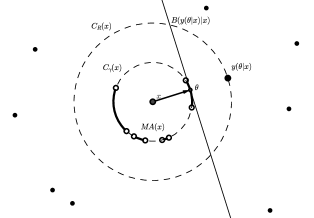
Figure 1: The black arcs represent the intervals of angles in $MA(x)$, whereas the open circles represent the open ends of these intervals.

To simplify the terms, let $W({\theta}|{x})=W({y({\theta}|{x})}|{x})$ and $B({\theta}|{x})=B({y({\theta}|{x})}|{x})$ in the remaining of this section. Also, let $F({\theta}|{x})$ be the line passing through $x$ and parallel to $B({\theta}|{x})$. The following lemma provides the basis for pruning.

Lemma 6

Let $x\in\mathbb{R}^{2}$ be an arbitrary point, and $\theta$ be an angle in $MA(x)$. For any point $x^{\prime}\notin H^{-}(F({\theta}|{x}),y({\theta}|{x}))$, $W^{*}(x^{\prime})\geq W^{*}(x)$.

Proof

Since $x^{\prime}\notin H^{-}(F({\theta}|{x}),y({\theta}|{x}))$ and $y({\theta}|{x})\in H^{-}(F({\theta}|{x}),y({\theta}|{x}))$, by the definition of bisectors, the distance between $F({\theta}|{x^{\prime}})$ and $B({\theta}|{x})$ is no less than $R/2$, which implies that $H^{-}(B({\theta}|{x}),y({\theta}|{x}))\subseteq H^{-}(B({\theta}|{x^{\prime}}),y({\theta}|{x^{\prime}}))$. Therefore, we can derive the following inequality

$$W^{*}(x^{\prime}) \geq W({\theta}|{x^{\prime}})$$

$$= W(H^{-}(B({\theta}|{x^{\prime}}),y({\theta}|{x^{\prime}}))$$

$$\geq W(H^{-}(B({\theta}|{x}),y({\theta}|{x}))$$

$$= W({\theta}|{x})$$

$$= W^{*}(x),$$

which completes the proof. ∎

This lemma tells us that, given a point $x$ and an angle $\theta\in MA(x)$, all points not in $H^{-}(F({\theta}|{x}),y({\theta}|{x}))$ can be ignored while finding $(1|1)_{R}$-centroids, as their weight losses are no less than that of $x$. By this lemma, we can also prove that the weight loss function is convex along any line on the plane, as shown below.

Lemma 7

Let $x_{1},x_{2}$ be two arbitrary distinct points on a given line $L$. For any point $x\in\overline{x_{1}x_{2}}\backslash\{x_{1},x_{2}\}$, $W^{*}(x)\leq\max\{W^{*}(x_{1}),W^{*}(x_{2})\}$.

Proof

Suppose by contradiction that $W^{*}(x)>W^{*}(x_{1})$ and $W^{*}(x)>W^{*}(x_{2})$ for some point $x\in\overline{x_{1}x_{2}}\backslash\{x_{1},x_{2}\}$. Since $W^{*}(x)>W^{*}(x_{1})$, by Lemma 6 there exists an angle $\theta\in MA(x)$ such that $x_{1}$ is included in $H^{-}(F({\theta}|{x}),y({\theta}|{x}))$. However, since $x\in\overline{x_{1}x_{2}}\backslash\{x_{1},x_{2}\}$, $x_{1}$ and $x_{2}$ locate on different sides of $F({\theta}|{x})$. It follows that $x_{2}$ is outside $H^{-}(F({\theta}|{x}),y({\theta}|{x}))$ and $W^{*}(x_{2})\geq W^{*}(x)$ by Lemma 6, which contradicts the assumption. Thus, the lemma holds. ∎

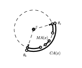
(a) $CA(x)$

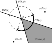
(b) $Wedge(x)$

Figure 2: $CA(x)$ and $Wedge(x)$.

We further investigate the distribution of angles in $MA(x)$. Let $CA(x)$ be the minimal angle interval covering all angles in $MA(x)$ (see Figure 2(a)), and $\delta(CA(x))$ be its angle span in radians. As mentioned before, $MA(x)$ consists of open angle interval(s) of non-zero length, which implies that $CA(x)$ is an open interval and $\delta(CA(x))>0$. Moreover, we can derive the following.

Lemma 8

If $\delta(CA(x))>\pi$, $x$ is a $(1|1)_{R}$-centroid.

Proof

We prove this lemma by showing that $W^{*}(x^{\prime})\geq W^{*}(x)\;\forall\;x^{\prime}\neq x$. Let $x^{\prime}\in\mathbb{R}^{2}$ be an arbitrary point other than $x$, and $\theta^{\prime}$ be its polar angle with respect to $x$. Obviously, any angle $\theta$ satisfying $x^{\prime}\in H^{-}(F({\theta}|{x}),y({\theta}|{x}))$ is in the open interval $(\theta^{\prime}-\pi/2,\theta^{\prime}+\pi/2)$, the angle span of which is equal to $\pi$. Since $\delta(CA(x))>\pi$, by its definition there exists an angle $\theta\in MA(x)$ such that $x^{\prime}\notin H^{-}(F({\theta}|{x}),y({\theta}|{x}))$. Thus, by Lemma 6, we have $W^{*}(x^{\prime})\geq W^{*}(x)$, thereby proves the lemma. ∎

We call a point $x$ satisfying Lemma 8 a strong $(1|1)_{R}$-centroid, since its discovery gives an immediate solution to the $(1|1)_{R}$-centroid problem. Note that there are problem instances in which no strong $(1|1)_{R}$-centroids exist.

Suppose that $\delta(CA(x))\leq\pi$ for some point $x\in\mathbb{R}^{2}$. Let $Wedge(x)$ denote the wedge of $x$, defined as the intersection of the two half-planes $H(F({\theta_{b}}|{x}),y({\theta_{b}}|{x}))$ and $H(F({\theta_{e}}|{x}),y({\theta_{e}}|{x}))$, where $\theta_{b}$ and $\theta_{e}$ are the beginning and ending angles of $CA(x)$, respectively. As illustrated in Figure 2(b), $Wedge(x)$ is the infinite region lying between two half-lines extending from $x$ (including $x$ and the two half-lines). The half-lines defined by $F({\theta_{e}}|{x})$ and $F({\theta_{b}}|{x})$ are called its boundaries, and the counterclockwise (CCW) angle between the two boundaries is denoted by $\delta(Wedge(x))$. Since $0<\delta(CA(x))\leq\pi$, we have that $Wedge(x)\neq\emptyset$ and $0\leq\delta(Wedge(x))<\pi$.

It should be emphasized that $Wedge(x)$ is a computational byproduct of $CA(x)$ when $x$ is not a strong $(1|1)_{R}$-centroid. In other words, not every point has its wedge. Therefore, we make the following assumption (or restriction) in order to avoid the misuse of $Wedge(x)$.

Assumption 1

Whenever $Wedge(x)$ is mentioned, the point $x$ has been found not to be a strong $(1|1)_{R}$-centroid, either by computation or by properties. Equivalently, $\delta(CA(x))\leq\pi$.

The following essential lemma makes $Wedge(x)$ our main tool for prune-and-search. (Note that its proof cannot be trivially derived from Lemma 6, since by definition $\theta_{b}$ and $\theta_{e}$ do not belong to the open intervals $CA(x)$ and $MA(x)$.)

Lemma 9

Let $x\in\mathbb{R}^{2}$ be an arbitrary point. For any point $x^{\prime}\notin Wedge(x)$, $W^{*}(x^{\prime})\geq W^{*}(x)$.

Proof

By symmetry, suppose that $x^{\prime}\notin H(F({\theta_{b}}|{x}),y({\theta_{b}}|{x}))$. We can further divide the position of $x^{\prime}$ into two cases, (1) $x^{\prime}\in H(F({\theta_{e}}|{x}),y({\theta_{e}}|{x}))$ and (2) $x^{\prime}\notin H(F({\theta_{e}}|{x}),y({\theta_{e}}|{x}))$.

Consider case (1). The two assumptions ensure that there exists an angle $\theta^{\prime}\in(\theta_{b},\theta_{e}]$, such that $F({\theta^{\prime}}|{x})$ passes through $x^{\prime}$. Obviously, any angle $\theta^{\prime\prime}\in(\theta_{b},\theta^{\prime})$ satisfies that $x^{\prime}\notin H(F({\theta^{\prime\prime}}|{x}),y({\theta^{\prime\prime}}|{x}))$. By the definition of $CA(x)$, there must exist an angle $\theta^{\prime}_{b}\in(\theta_{b},\theta^{\prime})$ infinitely close to $\theta_{b}$, such that $\theta^{\prime}_{b}$ belongs to $MA(x)$. Thus, by Lemma 6, we have that $W^{*}(x^{\prime})\geq W^{*}(x)$.

In case (2), for any angle $\theta^{\prime\prime}\in MA(x)$, we have that $x^{\prime}\notin H(F({\theta^{\prime\prime}}|{x}),y({\theta^{\prime\prime}}|{x}))$, since $\theta^{\prime\prime}$ is in $(\theta_{b},\theta_{e})$. Again, $W^{*}(x^{\prime})\geq W^{*}(x)$ by Lemma 6. ∎

Finally, we consider the computation of $Wedge(x)$.

Lemma 10

Given a point $x\in\mathbb{R}^{2}$, $MA(x)$, $CA(x)$, and $Wedge(x)$ can be computed in $O(n\log n)$ time.

Proof

By Theorem 2.1, we first compute $W^{*}(x)$ and those ordered tangent lines in $O(n\log n)$ time. Then, by performing angle sweeping around ${C_{\gamma}({x})}$, we can identify in $O(n)$ time those open intervals of angles $\theta$ with $W({\theta}|{x})=W^{*}(x)$, of which $MA(x)$ consists. Again by sweeping around ${C_{\gamma}({x})}$, $CA(x)$ can be obtained from $MA(x)$ in $O(n)$ time. Now, if we find $x$ to be a strong $(1|1)_{R}$-centroid by checking $\delta(CA(x))$, the $(1|1)_{R}$-centroid problem is solved and the algorithm can be terminated. Otherwise, $Wedge(x)$ can be constructed in $O(1)$ time. ∎

3.2 Searching on a Line

Although computing wedges can be used to prune candidate points, it does not serve as a stable prune-and-search tool, since wedges of different points have indefinite angle intervals and spans. However, Assumption 1 makes it work fine with lines. Here we show how to use the wedges to compute a local optimal point on a given line, i.e. a point $x$ with $W^{*}(x)\leq W^{*}(x^{\prime})$ for any point $x^{\prime}$ on the line.

Let $L$ be an arbitrary line, which is assumed to be non-horizontal for ease of discussion. For any point $x$ on $L$, we can compute $Wedge(x)$ and make use of it for pruning purposes by defining its direction with respect to $L$. Since $\delta(Wedge(x))<\pi$ by definition, there are only three categories of directions according to the intersection of $Wedge(x)$ and $L$:

Upward

– the intersection is the half-line of $L$ above and including $x$;

Downward

– the intersection is the half-line of $L$ below and including $x$;

Sideward

– the intersection is $x$ itself.

If $Wedge(x)$ is sideward, $x$ is a local optimal point on $L$, since by Lemma 9 $W^{*}(x)\leq W^{*}(x^{\prime})\;\forall\;x^{\prime}\in L$. Otherwise, either $Wedge(x)$ is upward or downward, the points on the opposite half of $L$ can be pruned by Lemma 9. It shows that computing wedges acts as a predictable tool for pruning on $L$.

Next, we list sets of breakpoints on $L$ in which a local optimal point locates. Recall that $\mathcal{T}$ is the set of outer tangent lines of all pairs of circles in $\mathcal{C}(V)$. We define the $\mathcal{T}$-breakpoints as the set $L\times\mathcal{T}$ of intersection points between $L$ and lines in $\mathcal{T}$, and the $\mathcal{C}$-breakpoints as the set $L\times\mathcal{C}(V)$ of intersection points between $L$ and circles in $\mathcal{C}(V)$. We have the following lemmas for breakpoints.

Lemma 11

Let $x_{1},x_{2}$ be two distinct points on $L$. If $W^{*}(x_{1})>W^{*}(x_{2})$, there exists at least a breakpoint on the segment $\overline{x_{1}x_{2}}\backslash\{x_{1}\}$.

Proof

Let $\theta$ be an arbitrary angle in $MA(x_{1})$ and $S$ be the subset of $V$ located in the half-plane $H^{-}(B({\theta}|{x_{1}}),y({\theta}|{x_{1}}))$. By definition, $x_{1}$ is outside the convex hull $CH(\mathcal{C}(S))$ and $W^{*}(x_{1})=W(S)$. On the other hand, since $W^{*}(x_{2})<W^{*}(x_{1})=W(S)$ by assumption, we have that $x_{2}$ is inside $CH(\mathcal{C}(S))$ by Lemma 2. Thus, the segment $\overline{x_{1}x_{2}}\backslash\{x_{1}\}$ intersects with the boundary of $CH(\mathcal{C}(S))$. Since the boundary of $CH(\mathcal{C}(S))$ consists of segments of lines in $\mathcal{T}$ and arcs of circles in $\mathcal{C}(V)$, the intersection point is either a $\mathcal{T}$-breakpoint or a $\mathcal{C}$-breakpoint, thereby proves the lemma. ∎

Lemma 12

There exists a local optimal point $x^{*}_{L}$ which is also a breakpoint.

Proof

Let $x^{*}_{L}$ be a local optimal point such that $W^{*}(x^{\prime})>W^{*}(x^{*}_{L})$ for some point $x^{\prime}$ adjacent to $x^{*}_{L}$ on $L$. Note that, if no such local optimal point exists, every point on $L$ must have the same weight loss and be local optimal, and the lemma holds trivially. If such $x^{*}_{L}$ and $x^{\prime}$ exist, by Lemma 11 there is a breakpoint on $\overline{x^{\prime}x^{*}_{L}}\backslash\{x^{\prime}\}$, which is $x^{*}_{L}$ itself. Thus, the lemma holds. ∎

We remark that outer tangent lines parallel to $L$ are exceptional cases while considering breakpoints. For any line $T\in\mathcal{T}$ that is parallel to $L$, either $T$ does not intersect with $L$ or they just coincide. In either case, $T$ is irrelevant to the finding of local optimal points, and should not be counted for defining $\mathcal{T}$-breakpoints.

Now, by Lemma 12, if we have all breakpoints on $L$ sorted in the decreasing order of their y-coordinates, a local optimal point can be found by performing binary search using wedges. Obviously, such sorted sequence can be obtained in $O(n^{2}\log n)$ time, since $|L\times\mathcal{T}|=O(n^{2})$ and $|L\times\mathcal{C}(V)|=O(n)$. However, in order to speed up the computations of local optimal points on multiple lines, alternatively we propose an $O(n^{2}\log n)$-time preprocessing, so that a local optimal point on any given line can be computed in $O(n\log^{2}n)$ time.

The preprocessing itself is very simple. For each point $v\in V$, we compute a sequence $P(v)$, consisting of points in $V\backslash\{v\}$ sorted in increasing order of their polar angles with respect to $v$. The computation for all $v\in V$ takes $O(n^{2}\log n)$ time in total. Besides, all outer tangent lines in $\mathcal{T}$ are computed in $O(n^{2})$ time. We will show that, for any given line $L$, $O(n)$ sorted sequences can be obtained from these pre-computed sequences in $O(n\log n)$ time, which can be used to replace a sorted sequence of all $\mathcal{T}$-breakpoints in the process of binary search.

For any two points $v\in V$ and $z\in\mathbb{R}^{2}$, let $T^{r}({z}|{v})$ be the outer tangent line of ${C_{\gamma}({v})}$ and ${C_{\gamma}({z})}$ to the right of the line from $v$ to $z$. Similarly, let $T^{l}({z}|{v})$ be the outer tangent line to the left. (See Figure 3.) Moreover, let $t^{r}_{L}({z}|{v})$ and $t^{l}_{L}({z}|{v})$ be the points at which $T^{r}({z}|{v})$ and $T^{l}({z}|{v})$ intersect with $L$, respectively. We partition $\mathcal{T}$ into $O(n)$ sets $\mathcal{T}^{r}(v)=\{T^{r}({v_{i}}|{v})|v_{i}\in V\backslash\{v\}\}$ and $\mathcal{T}^{l}(v)=\{T^{l}({v_{i}}|{v})|v_{i}\in V\backslash\{v\}\}$ for $v\in V$, and consider their corresponding $\mathcal{T}$-breakpoints independently. By symmetry, we only discuss the case about $L\times\mathcal{T}^{r}(v)$.

Figure 3: Outer tangent lines of $v$.

Lemma 13

For each $v\in V$, we can compute $O(1)$ sequences of $\mathcal{T}$-breakpoints on $L$, which satisfy the following conditions:

1. Each sequence is of length $O(n)$ and can be obtained in $O(\log n)$ time.

2. Breakpoints in each sequence are sorted in decreasing y-coordinates.

3. The union of breakpoints in all sequences form $L\times\mathcal{T}^{r}(v)$.

Proof

Without loss of generality, suppose that $v$ is either strictly to the right of $L$ or on $L$. Note that each point $v_{i}\in V\backslash\{v\}$ corresponds to exactly one outer tangent line $T^{r}({v_{i}}|{v})$, thereby exactly one breakpoint $t^{r}_{L}({v_{i}}|{v})$. Such one-to-one correspondence can be easily done in $O(1)$ time. Therefore, equivalently we are computing sequences of points in $V\backslash\{v\}$, instead of breakpoints.

In the following, we consider two cases about the relative position between $L$ and ${C_{\gamma}({v})}$, (1) $L$ intersects with ${C_{\gamma}({v})}$ at zero or one point, (2) $L$ intersects with ${C_{\gamma}({v})}$ at two points.

Case (1):

Let $\theta_{L}$ be the angle of the upward direction along $L$. See Figure 4(a). We classify the points in $V\backslash\{v\}$ by their polar angles with respect to $v$. Let $P_{1}(v)$ denote the sequence of those points with polar angles in the interval $(\theta_{L},\theta_{L}+\pi)$ and sorted in CCW order. Similarly, let $P_{2}(v)$ be the sequence of points with polar angles in $(\theta_{L}+\pi,\theta_{L})$ and sorted in CCW order. Obviously, $P_{1}(v)$ and $P_{2}(v)$ together satisfy condition (c). (Note that points with polar angles $\theta_{L}$ and $\theta_{L}+\pi$ are ignored, since they correspond to outer tangent lines parallel to $L$.)

By general position assumption, we can observe that, for any two distinct points $v_{i},v_{j}$ in $P_{1}(v)$, $t^{r}_{L}({v_{i}}|{v})$ is strictly above $t^{r}_{L}({v_{j}}|{v})$ if and only if $v_{i}$ precedes $v_{j}$ in $P_{1}(v)$. Thus, the ordering of points in $P_{1}(v)$ implicitly describes an ordering of their corresponding breakpoints in decreasing y-coordinates. Similarly, the ordering in $P_{2}(v)$ implies an ordering of corresponding breakpoints in decreasing y-coordinates. It follows that both $P_{1}(v)$ and $P_{2}(v)$ satisfy condition (b).

As for condition (a), both $P_{1}(v)$ and $P_{2}(v)$ are of length $O(n)$ by definition. Also, since we have pre-computed the sequence $P(v)$ as all points in $V\backslash\{v\}$ sorted in CCW order, $P_{1}(v)$ and $P_{2}(v)$ can be implicitly represented as concatenations of subsequences of $P(v)$. This can be done in $O(\log n)$ time by searching in $P(v)$ the foremost elements with polar angles larger than $\theta_{L}$ and $\theta_{L}+\pi$, respectively.

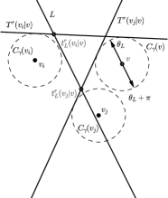
(a) no intersection

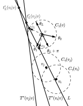
(b) two intersection points

Figure 4: Two subcases about how ${C_{\gamma}({v})}$ intersects $C$.

Case (2):

Suppose that the two intersection points between $L$ and ${C_{\gamma}({v})}$ are $c_{1}$ and $c_{2}$, where $c_{1}$ is above $c_{2}$. Let $\theta_{1}=\theta^{\prime}_{1}+\pi/2$ and $\theta_{2}=\theta^{\prime}_{2}+\pi/2$, in which $\theta^{\prime}_{1}$ and $\theta^{\prime}_{2}$ are respectively the polar angles of $c_{1}$ and $c_{2}$ with respect to $v$. See Figure 4(b). By assumption, we have that $\theta_{L}<\theta^{\prime}_{1}<\theta_{L}+\pi/2<\theta^{\prime}_{2}<\theta_{L}+\pi$, which implies that $\theta_{1}\in(\theta_{L},\theta_{L}+\pi)$ and $\theta_{2}\in(\theta_{L}+\pi,\theta_{L})$.

We divide the points in $V\backslash\{v\}$ into four sequences $P_{1}(v)$, $P_{2}(v)$, $P_{3}(v)$, and $P_{4}(v)$ by their polar angles with respect to $v$. $P_{1}(v)$ consists of points with polar angles in $(\theta_{L},\theta_{1})$, $P_{2}(v)$ in $[\theta_{1},\theta_{L}+\pi)$, $P_{3}(v)$ in $(\theta_{L}+\pi,\theta_{2}]$, and $P_{4}(v)$ in $(\theta_{2},\theta_{L})$, all sorted in CCW order. It follows that the four sequences satisfy conditions (c).

Condition (a) and (b) hold for $P_{1}(v)$ and $P_{4}(v)$ from similar discussion as above. However, for any two distinct points $v_{i},v_{j}$ in $P_{2}(v)$, we can observe that $t^{r}_{L}({v_{i}}|{v})$ is strictly below $t^{r}_{L}({v_{j}}|{v})$ if and only if $v_{i}$ precedes $v_{j}$ in $P_{2}(v)$. Similarly, the argument holds for $P_{3}(v)$. Thus, what satisfy condition (b) are actually the reverse sequences of $P_{2}(v)$ and $P_{3}(v)$, which can also be obtained in $O(\log n)$ time, satisfying condition (a). ∎

By Lemma 13.(c), searching in $L\times\mathcal{T}^{r}(v)$ is equivalent to searching in the $O(1)$ sequences of breakpoints, which can be computed more efficiently than the obvious way. Besides, we can also obtain a symmetrical lemma constructing sequences for $L\times\mathcal{T}^{l}(v)$. In the following, we show how to perform a binary search within these sequences.

Lemma 14

With an $O(n^{2}\log n)$-time preprocessing, given an arbitrary line $L$, a local optimal point $x^{*}_{L}$ can be computed in $O(n\log^{2}n)$ time.

Proof

By Lemma 12, the searching of $x^{*}_{L}$ can be done within $L\times\mathcal{T}$ and $L\times\mathcal{C}(V)$. $L\times\mathcal{T}$ can be further divided into $L\times\mathcal{T}^{r}(v)$ and $L\times\mathcal{T}^{l}(v)$ for each $v\in V$. By Lemma 13, these $2n$ sets can be replaced by $O(n)$ sorted sequences of breakpoints on $L$. Besides, $L\times\mathcal{C}(V)$ consists of no more than $2n$ breakpoints, which can be computed and arranged into a sorted sequence in decreasing y-coordinates. Therefore, we can construct $N_{0}=O(n)$ sequences $P_{1},P_{2},\cdots,P_{N_{0}}$ of breakpoints, each of length $O(n)$ and sorted in decreasing y-coordinates.

The searching in the $N_{0}$ sorted sequences is done by performing parametric search for parallel binary searches, introduced in [1]. The technique we used here is similar to the algorithm in [1], but uses a different weighting scheme. For each sorted sequence $P_{j}$, $1\leq j\leq N_{0}$, we first obtain its middle element $x_{j}$, and associate $x_{j}$ with a weight $m_{j}$ equal to the number of elements in $P_{j}$. Then, we compute the weighted median [18] of the $N_{0}$ middle elements, defined as the element $x$ such that $\sum\{m_{j}|x_{j}\text{ is above }x\}\geq\sum m_{j}/2$ and $\sum\{m_{j}|x_{j}\text{ is below }x\}\geq\sum m_{j}/2$. Finally, we apply Lemma 10 on the point $x$. If $x$ is a strong $(1|1)_{R}$-centroid, of course it is local optimal. If not, Assumption 1 holds and $Wedge(x)$ can be computed. If $Wedge(x)$ is sideward, a local optimal point $x^{*}_{L}=x$ is directly found. Otherwise, $Wedge(x)$ is either upward or downward, and thus all breakpoints on the opposite half can be pruned by Lemma 9. The pruning makes a portion of sequences, that possesses over half of total breakpoints by the definition of weighted median, lose at least a quarter of their elements. Hence, at least one-eighths of breakpoints are pruned. By repeating the above process, we can find $x^{*}_{L}$ in at most $O(\log n)$ iterations.

The time complexity for finding $x^{*}_{L}$ is analyzed as follows. By Lemma 13, constructing sorted sequences for $L\times\mathcal{T}^{r}(v)$ and $L\times\mathcal{T}^{l}(v)$ for all $v\in V$ takes $O(n\log n)$ time. Computing and sorting $L\times\mathcal{C}(V)$ also takes $O(n\log n)$ time. There are at most $O(\log n)$ iterations of the pruning process. At each iteration, the $N_{0}$ middle elements and their weighted median $x$ can be obtained in $O(N_{0})=O(n)$ time by the linear-time weighted selection algorithm [18]. Then, the computation of $Wedge(x)$ takes $O(n\log n)$ time by Lemma 10. Finally, the pruning of those sequences can be done in $O(n)$ time. In summary, the searching of $x^{*}_{L}$ requires $O(n\log n)+O(\log n)\times O(n\log n)=O(n\log^{2}n)$ time. ∎

We remark that, by Lemma 14, it is easy to obtain an intermediate result for the $(1|1)_{R}$-centroid problem on the plane. By Lemma 5, there exists a $(1|1)_{R}$-centroid in $\mathcal{T}\times\mathcal{T}$, $\mathcal{T}\times\mathcal{C}(V)$, and $\mathcal{C}(V)\times\mathcal{C}(V)$. By applying Lemma 14 to the $O(n^{2})$ lines in $\mathcal{T}$, the local optimum among the intersection points in $\mathcal{T}\times\mathcal{T}$ and $\mathcal{T}\times\mathcal{C}(V)$ can be obtained in $O(n^{3}\log^{2}n)$ time. By applying Theorem 2.1 on the $O(n^{2})$ intersection points in $\mathcal{C}(V)\times\mathcal{C}(V)$, the local optimum among them can be obtained in $O(n^{3}\log n)$ time. Thus, we can find a $(1|1)_{R}$-centroid in $O(n^{3}\log^{2}n)$ time, a nearly $O(n^{2})$ improvement over the $O(n^{5}\log n)$ bound in [5].

4 $(1|1)_{R}$-Centroid on the Plane

In this section, we study the $(1|1)_{R}$-centroid problem and propose an improved algorithm of time complexity $O(n^{2}\log n)$. This algorithm is as efficient as the best-so-far algorithm for the $(1|1)$-centroid problem, but based on a completely different approach.

In Subsection 4.1, we extend the algorithm of Lemma 14 to develop a procedure allowing us to prune candidate points with respect to a given vertical line. Then, in Subsection 4.2, we show how to compute a $(1|1)_{R}$-centroid in $O(n^{2}\log n)$ time based on this newly-developed pruning procedure.

4.1 Pruning with Respect to a Vertical Line

Let $L$ be an arbitrary vertical line on the plane. We call the half-plane strictly to the left of $L$ the left plane of $L$ and the one strictly to its right the right plane of $L$. A sideward wedge of some point on $L$ is said to be rightward (leftward) if it intersects the right (left) plane of $L$. We can observe that, if there is some point $x\in L$ such that $Wedge(x)$ is rightward, every point $x^{\prime}$ on the left plane of $L$ can be pruned, since $W^{*}(x^{\prime})\geq W^{*}(x)$ by Lemma 9. Similarly, if $Wedge(x)$ is leftward, points on the right plane of $L$ can be pruned. Although the power of wedges is not fully exerted in this way, pruning via vertical lines and sideward wedges is superior than directly via wedges due to predictable pruning regions.

Therefore, in this subsection we describe how to design a procedure that enables us to prune either the left or the right plane of a given vertical line $L$. As mentioned above, the key point is the searching of sideward wedges on $L$. It is achieved by carrying out three conditional phases. In the first phase, we try to find some proper breakpoints with sideward wedges. If failed, we pick some representative point in the second phase and check its wedge to determine whether or not sideward wedges exist. Finally, in case of their nonexistence, we show that their functional alternative can be computed, called the pseudo wedge, that still allows us to prune the left or right plane of $L$. In the following, we develop a series of lemmas to demonstrate the details of the three phases.

Property 1

Given a point $x\in L$, for each possible direction of $Wedge(x)$, the corresponding $CA(x)$ satisfies the following conditions:

Upward

– $CA(x)\subseteq(0,\pi)$,

Downward

– $CA(x)\subseteq(\pi,2\pi)$,

Rightward

– $0\in CA(x)$,

Leftward

– $\pi\in CA(x)$.

Proof

When $Wedge(x)$ is upward, by definition the beginning angle $\theta_{b}$ and the ending angle $\theta_{e}$ of $CA(x)$ must satisfy that both half-planes $H(F({\theta_{b}}|{x}),y({\theta_{b}}|{x}))$ and $H(F({\theta_{e}}|{x}),y({\theta_{e}}|{x}))$ include the half-line of $L$ above $x$. It follows that $0\leq\theta_{b},\theta_{e}\leq\pi$, and thus $CA(x)\subseteq(0,\pi)$. (Recall that $\theta_{b},\theta_{e}\notin CA(x)$.) The case that $Wedge(x)$ is downward can be proved in a symmetric way.

When $Wedge(x)$ is rightward, we can see that $H(F({\theta_{b}}|{x}),y({\theta_{b}}|{x}))$ must not contain the half-line of $L$ above $x$, and thus $\pi<\theta_{b}<2\pi$. By similar arguments, $0<\theta_{e}<\pi$. Therefore, counterclockwise covering angles from $\theta_{b}$ to $\theta_{e}$, $CA(x)$ must include the angle $0$. The case that $Wedge(x)$ is leftward can be symmetrically proved. ∎

Lemma 15

Let $x_{1},x_{2}$ be two points on $L$, where $x_{1}$ is strictly above $x_{2}$. For any angle $0\leq\theta\leq\pi$, $W({\theta}|{x_{1}})\leq W({\theta}|{x_{2}})$. Symmetrically, for $\pi\leq\theta\leq 2\pi$, $W({\theta}|{x_{2}})\leq W({\theta}|{x_{1}})$.

Proof

For any angle $0\leq\theta\leq\pi$, we can observe that $H^{-}(B({\theta}|{x_{1}}),y({\theta}|{x_{1}}))\subset H^{-}(B({\theta}|{x_{2}}),y({\theta}|{x_{2}}))$, since $x_{1}$ is strictly above $x_{2}$. It follows that $W({\theta}|{x_{1}})\leq W({\theta}|{x_{2}})$. The second claim also holds by symmetric arguments. ∎

Lemma 16

Let $x$ be an arbitrary point on $L$. If $Wedge(x)$ is either upward or downward, for any point $x^{\prime}\in L\backslash Wedge(x)$, $Wedge(x^{\prime})$ has the same direction as $Wedge(x)$.

Proof

By symmetry, we prove that, if $Wedge(x)$ is upward, $Wedge(x^{\prime})$ is also upward for every $x^{\prime}\in L$ strictly below $x$. By Property 1, the fact that $Wedge(x)$ is upward means that $CA(x)\subset(0,\pi)$ and thus $MA(x)\subset(0,\pi)$. Let $x^{\prime}$ be a point on $L$ strictly below $x$. By Lemma 15, we have that $W({\theta}|{x^{\prime}})\geq W({\theta}|{x})$ for $0<\theta<\pi$ and $W({\theta}|{x^{\prime}})\leq W({\theta}|{x})$ for $\pi\leq\theta\leq 2\pi$. It follows that $MA(x^{\prime})\subset(0,\pi)$ and $CA(x^{\prime})\subset(0,\pi)$, so $Wedge(x^{\prime})$ is upward as well. ∎

Following from this lemma, if there exist two arbitrary points $x_{1}$ and $x_{2}$ on $L$ with their wedges downward and upward, respectively, we can derive that $x_{1}$ must be strictly above $x_{2}$, and that points with sideward wedges or even strong $(1|1)_{R}$-centroids can locate only between $x_{1}$ and $x_{2}$. Thus, we can find sideward wedges between some specified downward and upward wedges. Let $x_{D}$ be the lowermost breakpoint on $L$ with its wedge downward, $x_{U}$ the uppermost breakpoint on $L$ with its wedge upward, and $G_{DU}$ the open segment $\overline{x_{D}x_{U}}\backslash\{x_{D},x_{U}\}$. (For ease of discussion, we assume that both $x_{D}$ and $x_{U}$ exist on $L$, and show how to resolve this assumption later by constructing a bounded box.) Again, $x_{D}$ is strictly above $x_{U}$. Also, we have the following corollary by their definitions.

Corollary 17

If there exist breakpoints in the segment $G_{DU}$, for any such breakpoint $x$, either $x$ is a strong $(1|1)_{R}$-centroid or $Wedge(x)$ is sideward.

Given $x_{D}$ and $x_{U}$, the first phase can thus be done by checking whether there exist breakpoints in $G_{DU}$ and picking any of them if exist. Supposing that the picked one is not a strong $(1|1)_{R}$-centroid, a sideward wedge is found by Corollary 17 and can be used for pruning. Notice that, when there are two or more such breakpoints, one may question whether their wedges are of the same direction, as different directions result in inconsistent pruning results. The following lemma answers the question in the positive.

Lemma 18

Let $x_{1}$, $x_{2}$ be two distinct points on $L$, where $x_{1}$ is strictly above $x_{2}$ and none of them is a strong $(1|1)_{R}$-centroid. If $Wedge(x_{1})$ and $Wedge(x_{2})$ are both sideward, they are either both rightward or both leftward.

Proof

We prove this lemma by contradiction. By symmetry, suppose the case that $Wedge(x_{1})$ is rightward and $Wedge(x_{2})$ is leftward. This case can be further divided into two subcases by whether or not $CA(x_{1})$ and $CA(x_{2})$ intersect.

Consider first that $CA(x_{1})$ does not intersect $CA(x_{2})$. Because $Wedge(x_{1})$ is rightward, $0\in CA(x_{1})$ by Property 1. Thus, there exists an angle $\theta$, $0<\theta<\pi$, such that $\theta\in MA(x_{1})$. Since $x_{1}$ is strictly above $x_{2}$, by Lemma 15 we have that $W^{*}(x_{1})=W({\theta}|{x_{1}})\leq W({\theta}|{x_{2}})\leq W^{*}(x_{2})$. Furthermore, since $Wedge(x_{2})$ is leftward, we can see that $x_{1}\notin Wedge(x_{2})$ and therefore $W^{*}(x_{1})\geq W^{*}(x_{2})$ by Lemma 9. It follows that $W({\theta}|{x_{2}})=W^{*}(x_{2})$ and thus $\theta\in MA(x_{2})$. By definition, $MA(x_{1})\subseteq CA(x_{1})$ and $MA(x_{2})\subseteq CA(x_{2})$, which implies that $CA(x_{1})$ and $CA(x_{2})$ intersect at $\theta$, contradicting the subcase assumption.

When $CA(x_{1})$ intersects $CA(x_{2})$, their intersection must be completely included in either $(0,\pi)$ or $(\pi,2\pi)$ due to Assumption 1. By symmetry, we assume the latter subcase. Using similar arguments as above, we can find an angle $\theta^{\prime}$, where $0<\theta^{\prime}<\pi$, such that $\theta^{\prime}\in MA(x_{1})$ and $\theta^{\prime}\in MA(x_{2})$. This is a contradiction, since $\theta^{\prime}\notin(\pi,2\pi)$.

Since both subcases do not hold, the lemma is proved. ∎

The second phase deals with the case that no breakpoint exists between $x_{D}$ and $x_{U}$ by determining the wedge direction of an arbitrary inner point in $G_{DU}$. We begin with several auxiliary lemmas.

Lemma 19

Let $x_{1},x_{2}$ be two distinct points on $L$ such that $W^{*}(x_{1})=W^{*}(x_{2})$ and $x_{1}$ is strictly above $x_{2}$. There exists at least one breakpoint in the segment

1. $\overline{x_{1}x_{2}}\backslash\{x_{2}\}$, if $MA(x_{2})$ intersects $(0,\pi)$ but $MA(x_{1})$ does not,

2. $\overline{x_{1}x_{2}}\backslash\{x_{1}\}$, if $MA(x_{1})$ intersects $(\pi,2\pi)$ but $MA(x_{2})$ does not.

Proof

By symmetry, we only show the correctness of condition (a). From its assumption, there exists an angle $\theta$, where $0<\theta<\pi$, such that $\theta\in MA(x_{2})$. Let $S=V\bigcap H^{-}(B({\theta}|{x_{2}}),y({\theta}|{x_{2}}))$. By definition, we have that $W(S)=W({\theta}|{x_{2}})=W^{*}(x_{2})=W^{*}(x_{1})$ and $CH(\mathcal{C}(S))\subset H^{-}(F({\theta}|{x_{2}}),y({\theta}|{x_{2}}))$, which implies that $CH(\mathcal{C}(S))$ is strictly above $F({\theta}|{x_{2}})$. (See Figure 5.)

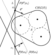
Figure 5: $CH(\mathcal{C}(S))$ intersects $L$ between $x_{1}$ and $x_{2}$.

We first claim that $CH(\mathcal{C}(S))$ intersects $L$. If not, there must exist an angle $\theta^{\prime}$, where $0<\theta^{\prime}<\pi$, such that $CH(\mathcal{C}(S))\subset H^{-}(F({\theta^{\prime}}|{x_{1}}),y({\theta^{\prime}}|{x_{1}}))$, that is, $S\subset H^{-}(B({\theta^{\prime}}|{x_{1}}),y({\theta^{\prime}}|{x_{1}}))$. By definition, $W^{*}(x_{1})\geq W({\theta^{\prime}}|{x_{1}})\geq W(S)$. Since $W^{*}(x_{1})=W(S)$, $W({\theta^{\prime}}|{x_{1}})=W^{*}(x_{1})$ and thus $\theta^{\prime}\in MA(x_{1})$, which contradicts the condition that $MA(x_{1})$ does not intersect $(0,\pi)$. Thus, the claim holds.

When $CH(\mathcal{C}(S))$ intersects $L$, $x_{1}$ locates either inside or outside $CH(\mathcal{C}(S))$. Since $x_{2}$ locates outside $CH(\mathcal{C}(S))$, in the former case the boundary of $CH(\mathcal{C}(S))$ intersects $\overline{x_{1}x_{2}}\backslash\{x_{2}\}$ and forms a breakpoint, thereby proves condition (a). On the other hand, if $x_{1}$ is outside $CH(\mathcal{C}(S))$, again there exists an angle $\theta^{\prime\prime}$ such that $CH(\mathcal{C}(S))\subset H^{-}(F({\theta^{\prime\prime}}|{x_{1}}),y({\theta^{\prime\prime}}|{x_{1}}))$. By similar arguments, we can show that $\theta^{\prime\prime}\in MA(x_{1})$. By assumption, $\theta^{\prime\prime}$ must belong to $(\pi,2\pi)$, which implies that $CH(\mathcal{C}(S))$ is strictly below $F({\theta^{\prime\prime}}|{x_{1}})$. Since $CH(\mathcal{C}(S))$ is strictly above $F({\theta}|{x_{2}})$ as mentioned, any intersection point between $CH(\mathcal{C}(S))$ and $L$ should be inner to $\overline{x_{1}x_{2}}$. Therefore, the lemma holds. ∎

Lemma 20

Let $G$ be a line segment connecting two consecutive breakpoints on $L$. For any two distinct points $x_{1},x_{2}$ inner to $G$, $W^{*}(x_{1})=W^{*}(x_{2})$.

Proof

Suppose to the contrary that $W^{*}(x_{1})\neq W^{*}(x_{2})$. By Lemma 11, there exists at least one breakpoint in $\overline{x_{1}x_{2}}$, which contradicts the definition of $G$. Thus, the lemma holds. ∎

Lemma 21

When there is no breakpoint between $x_{D}$ and $x_{U}$, any two distinct points $x_{1},x_{2}$ in $G_{DU}$ have the same wedge direction, if they are not strong $(1|1)_{R}$-centroids.

Proof

Suppose by contradiction that the directions of their wedges are different. By Lemmas 16 and 18, there are only two possible cases.

1. $Wedge(x_{1})$ is downward, and $Wedge(x_{2})$ is either sideward or upward.

2. $Wedge(x_{1})$ is sideward, and $Wedge(x_{2})$ is upward.

In the following, we show that both cases do not hold.

Case (1):

Because $Wedge(x_{1})$ is downward, we have that $CA(x_{1})\subseteq(\pi,2\pi)$ by Property 1 and thus $MA(x_{1})$ does not intersect $(0,\pi)$. On the other hand, whether $Wedge(x_{2})$ is sideward or upward, we can see that $CA(x_{2})$ and $MA(x_{2})$ intersect $(0,\pi)$ by again Property 1. Since $W^{*}(x_{1})=W^{*}(x_{2})$ by Lemma 20, the status of the two points satisfies the condition (a) of Lemma 19, so at least one breakpoint exists between $x_{1}$ and $x_{2}$. By definitions of $x_{1}$ and $x_{2}$, this breakpoint is inner to $G_{DU}$, thereby contradicts the assumption. Therefore, Case (1) does not hold.

Case (2):

The proof of Case (2) is symmetric to that of Case (1). The condition (b) of Lemma 19 can be applied similarly to show the existence of at least one breakpoint between $x_{1}$ and $x_{2}$, again a contradiction.

Combining the above discussions, we prove that the wedges of $x_{1}$ and $x_{2}$ are of the same direction, thereby completes the proof of this lemma. ∎

This lemma enables us to pick an arbitrary point in $G_{DU}$, e.g., the bisector point $x_{B}$ of $x_{D}$ and $x_{U}$, as the representative of all inner points in $G_{DU}$. If $x_{B}$ is not a strong $(1|1)_{R}$-centroid and $Wedge(x_{B})$ is sideward, the second phase finishes with a sideward wedge found. Otherwise, if $Wedge(x_{B})$ is downward or upward, we can derive the following and have to invoke the third phase.

Lemma 22

If there is no breakpoint between $x_{D}$ and $x_{U}$ and $Wedge(x_{B})$ is not sideward, there exist neither strong $(1|1)_{R}$-centroids nor points with sideward wedges on $L$.

Proof

By Lemma 16, this lemma holds for points not in $G_{DU}$. Without loss of generality, suppose that $Wedge(x_{B})$ is downward. For all points in $G_{DU}$ above $x_{B}$, the lemma holds by again Lemma 16.

Consider an arbitrary point $x\in\overline{x_{B}x_{U}}\backslash\{x_{B},x_{U}\}$. We first show that $x$ is not a strong $(1|1)_{R}$-centroid. Suppose to the contrary that $x$ really is. By definition, we have that $\delta(CA(x))>\pi$, and thus $CA(x)$ and $MA(x)$ intersect $(0,\pi)$. On the other hand, $CA(x_{B})$ and $MA(x_{B})$ do not intersect $(0,\pi)$ due to downward $Wedge(x_{B})$ and Property 1. Since $W^{*}(x_{B})=W^{*}(x)$ by Lemma 20, applying the condition (a) of Lemma 19 to $x_{B}$ and $x$ shows that at least one breakpoint exists between them, which contradicts the no-breakpoint assumption. Now that $x$ is not a strong $(1|1)_{R}$-centroid, it must have a downward wedge, as $x_{B}$ does by Lemma 21. Therefore, the lemma holds for all points on $L$. ∎

When $L$ satisfies Lemma 22, it consists of only points with downward or upward wedges, and is said to be non-leaning. Obviously, our pruning strategy via sideward wedges could not apply to such non-leaning lines. The third phase overcomes this obstacle by constructing a functional alternative of sideward wedges, called the pseudo wedge, on either $x_{D}$ or $x_{U}$, so that pruning with respect to $L$ is still achievable. Again, we start with auxiliary lemmas.

Lemma 23

If $L$ is non-leaning, the following statements hold:

1. $W^{*}(x_{D})\neq W^{*}(x_{U})$,

2. $W^{*}(x)=\max\{W^{*}(x_{D}),W^{*}(x_{U})\}$ for all points $x\in G_{DU}$.

Proof

We prove the correctness of statement (a) by contradiction, and suppose that $W^{*}(x_{D})=W^{*}(x_{U})$. Besides, the fact that $L$ is non-leaning implies that no breakpoint exists in $G_{DU}$. By Lemmas 22 and 21, the wedges of all points in $G_{DU}$ are of the same direction, either downward or upward. Suppose the downward case by symmetry, and pick an arbitrary point in $G_{DU}$, say, $x_{B}$. Since $Wedge(x_{B})$ is downward, we have that $MA(x_{B})$ does not intersect $(0,\pi)$. Oppositely, by definition $Wedge(x_{U})$ is upward, so $CA(x_{U})$ and $MA(x_{U})$ are included in $(0,\pi)$. Because $x_{B}$ is strictly above $x_{U}$ and $W^{*}(x_{D})=W^{*}(x_{U})$, according to the condition (a) of Lemma 19, there exists at least one breakpoint in $\overline{x_{B}x_{U}}\backslash\{x_{U}\}$, which is a contradiction. Therefore, statement (a) holds.

The proof of statement (b) is also done by contradiction. By symmetry, assume that $W^{*}(x_{D})>W^{*}(x_{U})$ in statement (a). Consider an arbitrary point $x\in G_{DU}$. By Lemma 7, we have that $W^{*}(x)\leq\max\{W^{*}(x_{D}),W^{*}(x_{U})\}=W^{*}(x_{D})$. Suppose that the equality does not hold. Then, by Lemma 11, at least one breakpoint exists in the segment $\overline{x_{D}x}\backslash\{x_{D}\}$, contradicting the no-breakpoint fact. Thus, $W^{*}(x)=W^{*}(x_{D})$ and statement (b) holds. ∎

Let $W_{1}=\max\{W^{*}(x_{D}),W^{*}(x_{U})\}$. We are going to define the pseudo wedge on either $x_{U}$ or $x_{D}$, depending on which one has the smaller weight loss. We consider first the case that $W^{*}(x_{D})>W^{*}(x_{U})$, and obtain the following.

Lemma 24

If $L$ is non-leaning and $W^{*}(x_{D})>W^{*}(x_{U})$, there exists one angle $\theta$ for $x_{U}$, where $\pi\leq\theta\leq 2\pi$, such that $W(H(B({\theta}|{x_{U}}),y({\theta}|{x_{U}})))\geq W_{1}$.

Proof

We first show that there exists at least a subset $S\subseteq V$ with $W(S)=W_{1}$, such that $x_{U}$ locates on the upper boundary of $CH(\mathcal{C}(S))$. Let $x$ be the point strictly above but arbitrarily close to $x_{U}$ on $L$. By Lemma 23, $W^{*}(x)=W_{1}$, hence $W^{*}(x)>W^{*}(x_{U})$ by case assumption. It follows that $x_{U}\in Wedge(x)$ by Lemma 9 and $Wedge(x)$ must be downward. By Property 1, we have that $CA(x)\subseteq(\pi,2\pi)$. Thus, there exists an angle $\theta^{\prime}\in MA(x)$, where $\pi<\theta^{\prime}<2\pi$, such that $W(H^{-}(B({\theta^{\prime}}|{x}),y({\theta^{\prime}}|{x})))=W({\theta^{\prime}}|{x})=W_{1}$.

Let $S=V\bigcap H^{-}(B({\theta^{\prime}}|{x}),y({\theta^{\prime}}|{x}))$. Since $W^{*}(x_{U})<W_{1}=W(S)$, $x_{U}$ is inside $CH(\mathcal{C}(S))$ by Lemma 2. Oppositely, by the definition of $S$, $x$ is outside the convex hull $CH(\mathcal{C}(S))$. It implies that $x_{U}$ is the topmost intersection point between $CH(\mathcal{C}(S))$ and $L$, hence on the upper boundary of $CH(\mathcal{C}(S))$. (It is possible that $x_{U}$ locates at the leftmost or the rightmost point of $CH(\mathcal{C}(S))$.)

The claimed angle $\theta$ is obtained as follows. Since $x_{U}$ is a boundary point of $CH(\mathcal{C}(S))$, there exists a line $F$ passing through $x_{U}$ and tangent to $CH(\mathcal{C}(S))$. Let $\theta$ be the angle satisfying that $F({\theta}|{x_{U}})=F$, $\pi\leq\theta\leq 2\pi$, and $CH(\mathcal{C}(S))\subset H(F({\theta}|{x_{U}}),y({\theta}|{x_{U}}))$. Obviously, we have that $S\subset H(B({\theta}|{x_{U}}),y({\theta}|{x_{U}}))$ and thus $W(H(B({\theta}|{x_{U}}),y({\theta}|{x_{U}})))\geq W^{*}(S)=W_{1}$. ∎

Let $\theta_{U}$ be an arbitrary angle satisfying the conditions of Lemma 24. We apply the line $F({\theta_{U}}|{x_{U}})$ for trimming the region of $Wedge(x_{U})$, so that a sideward wedge can be obtained. Let $PW(x_{U})$, called the pseudo wedge of $x_{U}$, denote the intersection of $Wedge(x_{U})$ and $H(F({\theta_{U}}|{x_{U}}),y({\theta_{U}}|{x_{U}}))$. Deriving from the three facts that $Wedge(x_{U})$ is upward, $\delta(Wedge(x_{U}))<\pi$, and $\pi\leq\theta_{U}\leq 2\pi$, we can observe that either $PW(x_{U})$ is $x_{U}$ itself, or it intersects only one of the right and left plane of $L$. In the two circumstances, $PW(x_{U})$ is said to be null or sideward, respectively. The pseudo wedge has similar functionality as wedges, as shown in the following corollary.

Corollary 25

For any point $x^{\prime}\notin PW(x_{U})$, $W^{*}(x^{\prime})\geq W^{*}(x_{U})$.

Proof

If $x^{\prime}\notin Wedge(x_{U})$, the lemma directly holds by Lemma 9. Otherwise, we have that $x^{\prime}\notin H(F({\theta}|{x_{U}}),y({\theta}|{x_{U}}))$ and thus $H(B({\theta}|{x^{\prime}}),y({\theta}|{x^{\prime}}))$ contains $H(B({\theta}|{x_{U}}),y({\theta}|{x_{U}}))$. Then, by Lemma 24, $W^{*}(x^{\prime})\geq W(H(B({\theta}|{x^{\prime}}),y({\theta}|{x^{\prime}})))\geq W(H(B({\theta}|{x_{U}}),y({\theta}|{x_{U}})))\geq W_{1}$, thereby completes the proof. ∎

By this lemma, if $PW(x_{U})$ is found to be sideward, points on the opposite half-plane with respect to $L$ can be pruned. If $PW(x_{U})$ is null, $x_{U}$ becomes another kind of strong $(1|1)_{R}$-centroids, in the meaning that it is also an immediate solution to the $(1|1)_{R}$-centroid problem. Without confusion, we call $x_{U}$ a conditional $(1|1)_{R}$-centroid in the latter case.

On the other hand, considering the reverse case that $W^{*}(x_{D})<W^{*}(x_{U})$, we can also obtain an angle $x_{D}$ and a pseudo wedge $PW(x_{D})$ for $x_{D}$ by symmetric arguments. Then, either $PW(x_{D})$ is sideward and the opposite side of $L$ can be pruned, or $PW(x_{D})$ itself is a conditional $(1|1)_{R}$-centroid. Thus, the third phase solves the problem of the nonexistence of sideward wedges.

Recall that the three phases of searching sideward wedges is based on the existence of $x_{D}$ and $x_{U}$ on $L$, which was not guaranteed before. Here we show that, by constructing appropriate border lines, we can guarantee the existence of $x_{D}$ and $x_{U}$ while searching between these border lines. The bounding box is defined as the smallest axis-aligned rectangle that encloses all circles in $\mathcal{C}(V)$. Obviously, any point $x$ outside the box satisfies that $W^{*}(x)=W(V)$ and must not be a $(1|1)_{R}$-centroid. Thus, given a vertical line not intersecting the box, the half-plane to be pruned is trivially decided. Moreover, let $T_{\text{top}}$ and $T_{\text{btm}}$ be two arbitrary horizontal lines strictly above and below the bounding box, respectively. We can obtain the following.

Lemma 26

Let $L$ be an arbitrary vertical line intersecting the bounding box, and $x^{\prime}_{D}$ and $x^{\prime}_{U}$ denote its intersection points with $T_{\text{top}}$ and $T_{\text{btm}}$, respectively. $Wedge(x^{\prime}_{D})$ is downward and $Wedge(x^{\prime}_{U})$ is upward.

Proof

Consider the case about $Wedge(x^{\prime}_{D})$. As described above, we know the fact that $W^{*}(x_{D})=W(V)$. Let $\theta$ be an arbitrary angle with $0\leq\theta\leq\pi$. We can observe that $H^{-}(F({\theta}|{x^{\prime}_{D}}),y({\theta}|{x^{\prime}_{D}}))$ cannot contain all circles in $\mathcal{C}(V)$, that is, $V\not\subset H^{-}(B({\theta}|{x^{\prime}_{D}}),y({\theta}|{x^{\prime}_{D}}))$. This implies that $W({\theta}|{x^{\prime}_{D}})<W^{*}(x^{\prime}_{D})$ and $\theta\notin MA(x^{\prime}_{D})$. Therefore, we have that $MA(x^{\prime}_{D})\subset(\pi,2\pi)$ and $Wedge(x^{\prime}_{D})$ is downward by Property 1. By similar arguments, we can show that $Wedge(x^{\prime}_{U})$ is upward. Thus, the lemma holds. ∎

According to this lemma, by inserting $T_{\text{top}}$ and $T_{\text{btm}}$ into $\mathcal{T}$, the existence of $x_{D}$ and $x_{U}$ is enforced for any vertical line intersecting the bounding box. Besides, it is obvious to see that the insertion does not affect the correctness of all lemmas developed so far.

Summarizing the above discussion, the whole picture of our desired pruning procedure can be described as follows. In the beginning, we perform a preprocessing to obtain the bounding box and then add $T_{\text{top}}$ and $T_{\text{btm}}$ into $\mathcal{T}$. Now, given a vertical line $L$, whether to prune its left or right plane can be determined by the following steps.

1. If $L$ does not intersect the bounding box, prune the half-plane not containing the box.

2. Compute $x_{D}$ and $x_{U}$ on $L$.

3. Find a sideward wedge or pseudo wedge via three forementioned phases. (Terminate whenever a strong or conditional $(1|1)_{R}$-centroid is found.)

   1. If breakpoints exist between $x_{D}$ and $x_{U}$, pick any of them and check it.

   2. If no such breakpoint, decide whether $L$ is non-leaning by checking $x_{B}$.

   3. If $L$ is non-leaning, compute $PW(x_{U})$ or $PW(x_{D})$ depending on which of $x_{U}$ and $x_{D}$ has smaller weight loss.

4. Prune the right or left plane of $L$ according to the direction of the sideward wedge or pseudo wedge.

The correctness of this procedure follows from the developed lemmas. Any vertical line not intersecting the bounding box is trivially dealt with in Step 1, due to the property of the box. When $L$ intersects the box, by Lemma 26, $x_{D}$ and $x_{U}$ can certainly be found in Step 2. The three sub-steps of Step 3 correspond to the three searching phases. When $L$ is not non-leaning, a sideward wedge is found, either at some breakpoint between $x_{D}$ and $x_{U}$ in Step 3(a) by Corollary 17, or at $x_{B}$ in Step 3(b) by Lemma 21. Otherwise, according to Lemma 24 or its symmetric version, a pseudo wedge can be built in Step 3(c) for $x_{U}$ or $x_{D}$, respectively. Finally in Step 4, whether to prune the left or right plane of $L$ can be determined via the just-found sideward wedge or pseudo wedge, by respectively Lemma 9 or Corollary 25.

The time complexity of this procedure is analyzed as follows. The preprocessing for computing the bounding box trivially takes $O(n)$ time. In Step 1, any vertical line not intersecting the box can be identified and dealt with in $O(1)$ time. Finding $x_{D}$ and $x_{U}$ in Step 2 requires the help of the binary-search algorithm developed in 3.2. Although the algorithm is designed to find a local optimal point, we can easily observe that slightly modifying its objective makes it applicable to this purpose without changing its time complexity. Thus, Step 2 can be done in $O(n\log^{2}n)$ time by Lemma 14.

In Step 3(a), all breakpoints between $x_{D}$ and $x_{U}$ can be found in $O(n\log n)$ time as follows. As done in Lemma 14, we first list all breakpoints on $L$ by $O(n)$ sorted sequences of length $O(n)$, which takes $O(n\log n)$ time. Then, by performing binary search with the y-coordinates of $x_{D}$ and $x_{U}$, we can find within each sequence the breakpoints between them in $O(\log n)$ time. In Step 3(a) or 3(b), checking a picked point $x$ is done by computing $CA(x)$, that requires $O(n\log n)$ time by Lemma 10. To compute the pseudo wedge in Step 3(c), the angle $\theta_{U}$ satisfying Lemma 24, or symmetrically $\theta_{D}$, can be computed in $O(n\log n)$ time by sweeping technique as in Lemma 10. Thus, $PW(x_{U})$ or $PW(x_{D})$ can be computed in $O(n\log n)$ time. Finally, the pruning decision in Step 4 takes $O(1)$ time. Summarizing the above, these steps require $O(n\log^{2}n)$ time in total. Since the invocation of Lemma 14 needs an additional $O(n^{2}\log n)$-time preprocessing, we have the following result.

Lemma 27

With an $O(n^{2}\log n)$-time preprocessing, whether to prune the right or left plane of a given vertical line $L$ can be determined in $O(n\log^{2}n)$ time.

4.2 Searching on the Euclidean Plane

In this subsection, we come back to the $(1|1)_{R}$-centroid problem. Recall that, by Lemma 5, at least one $(1|1)_{R}$-centroid can be found in the three sets of intersection points $\mathcal{T}\times\mathcal{T}$, $\mathcal{C}(V)\times\mathcal{T}$, and $\mathcal{C}(V)\times\mathcal{C}(V)$, which consist of total $O(n^{4})$ points. Let $\mathcal{L}$ denote the set of all vertical lines passing through these $O(n^{4})$ intersection points. By definition, there exists a vertical line $L^{*}\in\mathcal{L}$ such that its local optimal point is a $(1|1)_{R}$-centroid. Conceptually, with the help of Lemma 27, $L^{*}$ can be derived by applying prune-and-search approach to $\mathcal{L}$: pick the vertical line $L$ from $\mathcal{L}$ with median x-coordinates, determine by Lemma 27 whether the right or left plane of $L$ should be pruned, discard lines of $\mathcal{L}$ in the pruned half-plane, and repeat above until two vertical lines left. Obviously, it costs too much if this approach is carried out by explicitly generating and sorting the $O(n^{4})$ lines. However, by separately dealing with each of the three sets, we can implicitly maintain sorted sequences of these lines and apply the prune-and-search approach.

Let $\mathcal{L_{T}}$, $\mathcal{L_{M}}$, and $\mathcal{L_{C}}$ be the sets of all vertical lines passing through the intersection points in $\mathcal{T}\times\mathcal{T}$, $\mathcal{C}(V)\times\mathcal{T}$, and $\mathcal{C}(V)\times\mathcal{C}(V)$, respectively. A local optimal line of $\mathcal{L_{T}}$ is a vertical line $L_{t}^{*}$ such that its local optimal point has weight loss no larger than those of points in $\mathcal{T}\times\mathcal{T}$. The local optimal lines $L_{m}^{*}$ and $L_{c}^{*}$ can be similarly defined for $\mathcal{L_{M}}$ and $\mathcal{L_{C}}$, respectively. We will adopt different prune-and-search techniques to find the local optimal lines in the three sets, as shown in the following lemmas.

Lemma 28

A local optimal line $L_{t}^{*}$ of $\mathcal{L_{T}}$ can be found in $O(n^{2}\log n)$ time.

Proof

Let $N_{1}=|\mathcal{T}|$. By definition, there are $(N_{1})^{2}$ intersection points in $\mathcal{T}\times\mathcal{T}$ and $(N_{1})^{2}$ vertical lines in $\mathcal{L_{T}}$. For efficiently searching within these vertical lines, we apply the ingenious idea of parametric search via parallel sorting algorithms, proposed by Megiddo [15].

Consider two arbitrary lines $T_{g},T_{h}\in\mathcal{T}$. If they are not parallel, let $t_{gh}$ be their intersection point and $L_{gh}$ be the vertical line passing through $t_{gh}$. Suppose that $T_{g}$ is above $T_{h}$ in the left plane of $L_{gh}$. If applying Lemma 27 to $L_{gh}$ prunes its right plane, $T_{g}$ is above $T_{h}$ in the remained left plane. On the other hand, if the left plane of $L_{gh}$ is pruned, $T_{h}$ is above $T_{g}$ in the remained right plane. Therefore, $L_{gh}$ can be treated as a “comparison” between $T_{g}$ and $T_{h}$, in the sense that applying Lemma 27 to $L_{gh}$ determines their ordering in the remained half-plane. It also decides the ordering of their intersection points with the undetermined local optimal line $L_{t}^{*}$, since the pruning ensures that a local optimal line stays in the remained half-plane.

It follows that, by resolving comparisons, the process of pruning vertical lines in $\mathcal{L_{T}}$ to find $L_{t}^{*}$ can be reduced to the problem of determining the ordering of the intersection points of the $N_{1}$ lines with $L_{t}^{*}$, or say, the sorting of these intersection points on $L_{t}^{*}$. While resolving comparisons during the sorting process, we can simultaneously maintain the remained half-plane by two vertical lines as its boundaries. Thus, after resolving all comparisons in $\mathcal{L_{T}}$, one of the two boundaries must be a local optimal line. As we know, the most efficient way to obtain the ordering is to apply some optimal sorting algorithm $A_{S}$, which needs to resolve only $O(N_{1}\log N_{1})$ comparisons, instead of $(N_{1})^{2}$ comparisons. Since resolving each comparison takes $O(n\log^{2}n)$ time by Lemma 27, the sorting is done in $O(n\log^{2}n)\times O(N_{1}\log^{2}N_{1})=O(n^{3}\log^{3}n)$ time, so is the finding of $L_{t}^{*}$.

However, Megiddo [15] observed that, when multiple comparisons can be indirectly resolved in a batch, simulating parallel sorting algorithms in a sequential way naturally provides the scheme for batching comparisons, thereby outperform the case of applying $A_{S}$. Let $A_{P}$ be an arbitrary cost-optimal parallel sorting algorithm that runs in $O(\log n)$ steps on $O(n)$ processors, e.g., the parallel merge sort in [2]. Using $A_{P}$ to sort the $N_{1}$ lines in $\mathcal{L_{T}}$ on $L_{t}^{*}$ takes $O(\log N_{1})$ parallel steps. At each parallel step, there are $k=O(N_{1})$ comparisons $L_{1},L_{2},\cdots,L_{k}$ to be resolved. We select the one with median x-coordinate among them, which is supposed to be some $L_{i}$. If applying Lemma 27 to $L_{i}$ prunes its left plane, for each comparison $L_{j}$ to the left of $L_{i}$, the ordering of the corresponding lines of $L_{j}$ in the remained right plane of $L_{i}$ is directly known. Thus, the $O(k/2)$ comparisons to the left of $L_{i}$ are indirectly resolved in $O(k/2)$ time. If otherwise the right plane of $L_{i}$ is pruned, the $O(k/2)$ comparisons to its right are resolved in $O(k/2)$ time. By repeating this process of selecting medians and pruning on the remaining elements $O(\log k)$ times, all $k$ comparisons can be resolved, which takes $O(n\log^{2}n)\times O(\log k)+O(k+k/2+k/4+\cdots)=O(n\log^{3}n)+O(N_{1})=O(n^{2})$ time. Therefore, going through $O(\log N_{1})$ parallel steps of $A_{P}$ requires $O(n^{2}\log N_{1})=O(n^{2}\log n)$ time, which determines the ordering of lines in $\mathcal{L_{T}}$ on $L_{t}^{*}$ and also computes a local optimal line $L_{t}^{*}$. ∎

Lemma 29

A local optimal line $L_{m}^{*}$ of $\mathcal{L_{M}}$ can be found in $O(n^{2}\log n)$ time.

Proof

To deal with the set $\mathcal{L_{M}}$, we use the ideas similar to the proofs of Lemmas 13 and 14 in order to divide $\mathcal{C}(V)\times\mathcal{T}$ into sorted sequences of points. Given a fixed circle $C={C_{\gamma}({u_{0}})}$ for some point $u_{0}\in V$, we show that the intersection points in $C\times\mathcal{T}^{r}(v)$ and $C\times\mathcal{T}^{l}(v)$ for each $v\in V$ can be grouped into $O(1)$ sequences of length $O(n)$, which are sorted in increasing x-coordinates. Summarizing over all circles in $\mathcal{C}(V)$, there will be total $O(n^{2})$ sequences of length $O(n)$, each of which maps to a sequence of $O(n)$ vertical lines sorted in increasing x-coordinates. Then, finding a local optimal line $L_{m}^{*}$ can be done by performing prune-and-search to the $O(n^{2})$ sequences of vertical lines via parallel binary searches. The details of these steps are described as follows.

First we discuss about the way for grouping intersection points in $C\times\mathcal{T}^{r}(v)$ and $C\times\mathcal{T}^{l}(v)$ for a fixed point $v\in V$, so that each of them can be represented by $O(1)$ subsequences of $P(v)$. By symmetry, only $C\times\mathcal{T}^{r}(v)$ is considered. Similar to Lemma 13, we are actually computing sequences of points in $V\backslash\{v\}$ corresponding to these intersection points. For each $v_{i}\in V\backslash\{v\}$, the outer tangent line $T^{r}({v_{i}}|{v})$ may intersect $C$ at two, one, or zero point. Let $t^{r}_{C,1}({v_{i}}|{v})$ and $t^{r}_{C,2}({v_{i}}|{v})$ denote the first and second points, respectively, at which $T^{r}({v_{i}}|{v})$ intersects $C$ along the direction from $v$ to $v_{i}$. Note that, when $T^{r}({v_{i}}|{v})$ intersects $C$ at less than two points, $t^{r}_{C,2}({v_{i}}|{v})$ or both of them will be null.

In the following, we consider the sequence computation under two cases about the relationship between $u_{0}$ and $v$, (1) $u_{0}=v$, and (2) $u_{0}\neq v$.

Case (1):

Since $v$ coincides with $u_{0}$, $C\times\mathcal{T}^{r}(v)$ is just the set of tangent points $t^{r}_{C,1}({v_{i}}|{v})$ for all $v_{i}\in V\backslash\{v\}$. It is easy to see the the angular sorted sequence $P(v)$ directly corresponds to a sorted sequence of these $n-1$ tangent points in CCW order. $P(v)$ can be further partitioned into two sub-sequences $P_{1}(v)$ and $P_{2}(v)$, which consist of points in $V\backslash\{v\}$ with polar angles (with respect to $v$) in the intervals $[0,\pi)$ and $[\pi,2\pi)$, respectively. Since they are sorted in CCW order, we have that intersection points corresponding to $P_{2}(v)$ and to the reverse of $P_{1}(v)$ are sorted in increasing x-coordinates, as we required. Obviously, $P_{1}(v)$ and $P_{2}(v)$ are of length $O(n)$ and can be obtained in $O(\log n)$ time.

Case (2):

Suppose without loss of generality that $v$ locates on the lower left quadrant with respect to $u_{0}$, and let $\theta_{0}$ be the polar angle of $u_{0}$ with respect to $v$. This case can be further divided into two subcases by whether or not ${C_{\gamma}({v})}$ intersects $C$ at less than two points.

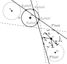
(a) no intersection

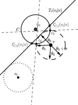
(b) two intersection points

Figure 6: Two subcases about how ${C_{\gamma}({v})}$ intersects $C$.

Consider first the subcase that they intersect at none or one point (see Figure 6(a).) Let $\theta_{3}$ and $\theta_{4}$ be the angles such that $T^{r}({y({\theta_{3}}|{v})}|{v})$ and $T^{r}({y({\theta_{4}}|{v})}|{v})$ are inner tangent to ${C_{\gamma}({v})}$ and $C$, where $\theta_{3}\leq\theta_{4}$ (Note that $\theta_{3}=\theta_{4}$ only when the two circles intersect at one point.) For each $v_{i}\in V\backslash\{v\}$, $T^{r}({v_{i}}|{v})$ does not intersect $C$, if the polar angle of $v_{i}$ with respect to $v$ is neither in $[\theta_{0},\theta_{3}]$ nor in $[\theta_{4},\theta_{0}+\pi]$. We can implicitly obtain from $P(v)$ two subsequences $P_{3}(v)$ and $P_{4}(v)$, consisting of points with polar angles in $[\theta_{0},\theta_{3}]$ and in $[\theta_{4},\theta_{0}+\pi]$, respectively. It can be observed that the sequence of points $v_{i}$ listed in $P_{3}(v)$ corresponds to a sequence of intersection points $t^{r}_{C,1}({v_{i}}|{v})$ listed in clockwise (CW) order on $C$ and, moreover, a sequence of $t^{r}_{C,2}({v_{i}}|{v})$ listed in CCW order on $C$. Symmetrically, the sequence of points $v_{j}$ in $P_{4}(v)$ corresponds to a sequence of $t^{r}_{C,1}({v_{j}}|{v})$ in CCW order and a sequence of $t^{r}_{C,2}({v_{j}}|{v})$ in CW order. The four implicit sequences of intersection points on $C$ can be further partitioned by a horizontal line $L_{h}$ passing through its center $u_{0}$, so that the resulted sequences are naturally sorted in either increasing or decreasing x-coordinates. Therefore, we can implicitly obtain at most eight sorted sequences of length $O(n)$ in replace of $C\times\mathcal{T}^{r}(v)$, by appropriately partitioning $P(v)$ in $O(\log n)$ time.

Consider that ${C_{\gamma}({v})}$ intersects ${C_{\gamma}({u_{0}})}$ at two points $c_{5}$ and $c_{6}$, where $c_{5}$ is to the upper right of $c_{6}$ (see Figure 6(b).) Let $\theta_{5}$ and $\theta_{6}$ be the angles such that $T^{r}({y({\theta_{5}}|{v})}|{v})$ and $T^{r}({y({\theta_{6}}|{v})}|{v})$ are tangent to ${C_{\gamma}({v})}$ at $c_{5}$ and $c_{6}$, respectively. Again, $P(v)$ can be implicitly partitioned into three subsequences $P_{5}(v)$, $P_{6}(v)$, and $P_{7}(v)$, which consists of points with polar angles in $[\theta_{0},\theta_{5})$, $[\theta_{5},\theta_{6})$, and $[\theta_{6},\theta_{0}+\pi]$, respectively. By similar observations, $P_{5}(v)$ corresponds to two sequences of intersection points listed in CW and CCW order, respectively, and $P_{7}(v)$ corresponds to two sequences listed in CCW and CW order, respectively. However, the sequence of points $v_{i}$ in $P_{6}(v)$ corresponds to the sequences of $t^{r}_{C,1}({v_{i}}|{v})$ and $t^{r}_{C,2}({v_{i}}|{v})$ listed in both CCW order. These sequences can also be partitioned by $L_{h}$ into sequences sorted in x-coordinates. It follows that we can implicitly obtain at most twelve sorted sequences of length $O(n)$ in replace of $C\times\mathcal{T}^{r}(v)$ in $O(\log n)$ time.

According to the above discussion, for any two points $u,v\in V$, ${C_{\gamma}({u})}\times\mathcal{T}^{r}(v)$ and ${C_{\gamma}({u})}\times\mathcal{T}^{l}(v)$ can be divided into $O(1)$ sequences in $O(\log n)$ time, each of which consists of $O(n)$ intersection points on ${C_{\gamma}({u})}$ sorted in increasing x-coordinates. Thus, $\mathcal{C}(V)\times\mathcal{T}$ can be re-organized as $O(n^{2})$ sorted sequences of length $O(n)$ in $O(n^{2}\log n)$ time, which correspond to $O(n^{2})$ sorted sequences of $O(n)$ vertical lines. Now, we can perform parametric search for parallel binary search to these sequences of vertical lines, by similar techniques used in Lemma 14. For each of the $O(n^{2})$ sequences, its middle element is first obtained and assigned with a weight equal to the sequence length in $O(1)$ time. Then, the weighted median $L$ of these $O(n^{2})$ elements are computed in $O(n^{2})$ time [18]. By applying Lemma 27 to $L$ in $O(n\log^{2}n)$ time, at least one-eighths of total elements can be pruned from these sequences, taking another $O(n^{2})$ time. Therefore, a single iteration of pruning requires $O(n^{2})$ time. After $O(\log n)$ such iterations, a local optimal line $L_{m}^{*}$ can be found in total $O(n^{2}\log n)$ time, thereby proves the lemma. ∎

Lemma 30

A local optimal line $L_{c}^{*}$ of $\mathcal{L_{C}}$ can be found in $O(n^{2}\log n)$ time.

Proof

There are at most $O(n^{2})$ points in $\mathcal{C}(V)\times\mathcal{C}(V)$. Thus, $\mathcal{L_{C}}$ can be obtained and sorted according to x-coordinates in $O(n^{2}\log n)$ time. Then, by simply performing binary search with Lemma 27, a local optimal line $L_{c}^{*}$ can be easily found in $O(\log n)$ iterations of pruning, which require total $O(n\log^{3}n)$ time. In summary, the computation takes $O(n^{2}\log n)$ time, and the lemma holds. ∎

By definition, $L^{*}$ can be found among $L_{t}^{*}$, $L_{m}^{*}$, and $L_{c}^{*}$, which can be computed in $O(n^{2}\log n)$ time by Lemmas 28, 29, and 30, respectively. Then, a $(1|1)_{R}$-centroid can be computed as the local optimal point of $L^{*}$ in $O(n\log^{2}n)$ time by Lemma 14. Combining with the $O(n^{2}\log n)$-time preprocessing for computing the angular sorted sequence $P(v)$s and the bounding box enclosing $\mathcal{C}(V)$, we have the following theorem.

Theorem 4.1

The $(1|1)_{R}$-centroid problem can be solved in $O(n^{2}\log n)$ time.

5 Concluding Remarks

In this paper, we revisited the $(1|1)$-centroid problem on the Euclidean plane under the consideration of minimal distance constraint between facilities, and proposed an $O(n^{2}\log n)$-time algorithm, which close the bound gap between this problem and its unconstrained version. Starting from a critical observation on the medianoid solutions, we developed a pruning tool with indefinite region remained after pruning, and made use of it via multi-level structured parametric search approach, which is quite different to the previous approach in [5, 11].

Considering distance constraint between facilities in various competitive facility location models is both of theoretical interest and of practical importance. However, similar constraints are rarely seen in the literature. It would be good starting points by introducing the constraint to the facilities between players in the $(r|X_{p})$-medianoid and $(r|p)$-centroid problems, maybe even to the facilities between the same player.

References

- [1] R. Cole, “Slowing down sorting networks to obtain faster sorting algorithms,” Journal of the ACM, vol. 34, no. 1, pp. 200–208, 1987.
- [2] R. Cole, “Parallel merge sort,” SIAM Journal on Computing, vol. 17, no. 4, pp. 770–785, 1988.
- [3] A. Dasci, “Conditional Location Problems on Networks and in the Plane,” In: H. A. Eiselt, V. Marianov (eds.), Foundations of Location Analysis, Springer, New York, pp. 179–206, 2011.
- [4] I. Davydov, Y. Kochetov, and A. Plyasunov, “On the complexity of the -centroid problem in the plane,” TOP, vol. 22, no. 2, pp. 614–623, 2013.
- [5] Z. Drezner, “Competitive location strategies for two facilities,” Regional Science and Urban Economics, vol 12, no. 4, pp. 485–493, 1982.
- [6] Z. Drezner, and Z. Eitan, “Competitive location in the plane,” Annals of Operations Research, vol. 40, no. 1, pp. 173–193, 1992.
- [7] H. A. Eiselt and G. Laporte, “Sequential location problems,” European Journal of Operational Research, vol. 96, pp. 217–231, 1997.
- [8] H. A. Eiselt, G. Laporte, and J.-F. Thisse, “Competitive location models: a framework and bibliography,” Transportation Science, vol. 27, pp. 44–54, 1993.
- [9] H. A. Eiselt, V. Marianov, Vladimir and T. Drezner, Tammy, “Competitive Location Models,” In: G. Laporte, S. Nickel, F. Saldanha da Gama (eds.), Location Science, Springer International Publishing, pp. 365–398, 2015.
- [10] S. L. Hakimi, “On locating new facilities in a competitive environment,” European Journal of Operational Research, vol. 12, no. 1, pp. 29–35, 1983.
- [11] S. L. Hakimi, “Locations with spatial interactions: competitive locations and games,” In: P.B. Mirchandani, R.L. Francis (eds), Discrete location theory, Wiley, New York, pp. 439–478, 1990.
- [12] P. Hansen, J.-F. Thisse, and R. W. Wendell, “Equilibrium analysis for voting and competitive location problems,” In: P. B. Mirchandani, R. L. Francis RL (eds), Discrete location theory, Wiley, New York, pp 479–501, 1990.
- [13] H. Hotelling, “Stability in competition,” Economic Journal, vol. 39, 41–57, 1929.
- [14] D. T. Lee, Y. F. Wu, “Geometric complexity of some location problems,” Algorithmica, vol. 1, no. 1, pp. 193–211, 1986.
- [15] N. Megiddo, “Applying parallel computation algorithms in the design of serial algorithms,” Journal of the ACM, vol. 30, no. 4, pp. 852–865, 1983.
- [16] N. Megiddo, “Linear-time algorithms for linear programming in and related problems,” SIAM Journal on Computing, vol. 12, no. 4, pp. 759–776, 1983.
- [17] F. Plastria, “Static competitive facility location: an overview of optimisation approaches.” European Journal of Operational Research, vol. 129, no. 3, pp. 461–470, 2001.
- [18] A. Reiser, “A linear selection algorithm for sets of elements with weights,” Information Processing Letters, vol. 7, no. 3, pp. 159–162, 1978.
- [19] D. R. Santos-Peñate, R. Suárez-Vega, and P. Dorta-González, “The leader–follower location model,” Networks and Spatial Economics, vol. 7, no. 1, pp. 45–61, 2007.