NEOSurvey 1: Initial results from the Warm Spitzer Exploration Science Survey of Near Earth Object Properties

Abstract

Near Earth Objects (NEOs) are small Solar System bodies whose orbits bring them close to the Earth’s orbit. We are carrying out a Warm Spitzer Cycle 11 Exploration Science program entitled NEOSurvey — a fast and efficient flux-limited survey of 597 known NEOs in which we derive diameter and albedo for each target. The vast majority of our targets are too faint to be observed by NEOWISE, though a small sample has been or will be observed by both observatories, which allows for a cross-check of our mutual results. Our primary goal is to create a large and uniform catalog of NEO properties. We present here the first results from this new program: fluxes and derived diameters and albedos for 80 NEOs, together with a description of the overall program and approach, including several updates to our thermal model. The largest source of error in our diameter and albedo solutions, which derive from our single band thermal emission measurements, is uncertainty in $\eta$, the beaming parameter used in our thermal modeling; for albedos, improvements in Solar System absolute magnitudes would also help significantly. All data and derived diameters and albedos from this entire program are being posted on a publicly accessible webpage at nearearthobjects.nau.edu .

1 Introduction

Near Earth Objects (NEOs) are small Solar System bodies whose orbits bring them close to the Earth’s orbit. NEOs lie at the intersection of science, space exploration, and civil defense. Because NEOs are constantly being replenished from sources elsewhere in the Solar System, they act as compositional and dynamical tracers and allow us to probe environmental conditions throughout the Solar System and the history of our planetary system. NEOs are the parent bodies of meteorites, one of our key sources of detailed knowledge about the Solar System’s development, and NEO studies provide the needed context for this work. The space exploration of NEOs is carried out both through robotic spacecraft such as NEAR (Veverka et al., 2001); Hayabusa (Fujiwara et al., 2006); Chang’e 2 (Ji et al., 2016); Hayabusa 2 (Abe et al., 2012); and OSIRIS-REx (Lauretta et al., 2015); as well as remote sensing observations using IRAS, Spitzer, WISE/NEOWISE, Akari, and other assets (as reviewed in Mainzer et al. 2015). Energetically, some NEOs are easier to reach with spacecraft than the Earth’s moon (Barbee et al., 2013), and NEOs offer a large number of targets with a range of physical properties and histories. NEOs present advanced astronautical challenges, and President Obama announced in 2010 that missions to asteroids would form the cornerstone of NASA’s exploration for the next decade or more; the new Asteroid Retrieval Mission (Abell et al., 2016) is part of those activities. Finally, NEOs are a civil defense matter: the impact threat from NEOs is real, as demonstrated again recently in Chelyabinsk, Russia, in February, 2013 (Popova et al., 2013; Brown et al., 2013). Understanding the number and properties of NEOs affects our planning strategies, international cooperation, and overall risk assessment.

The Spitzer Space Telescope is a powerful NEO characterization system. NEOs typically have daytime temperatures around 300 K. Hence, their thermal emission at 4.5 microns is almost always significantly larger than their reflected light at that wavelength. We can therefore employ a thermal model to derive NEO properties, with the primary result being derived diameters and albedos (Trilling et al., 2010). Measuring the size distribution and albedos and compositions for a large fraction of all known NEOs allows us to understand the scientific, exploration, and civil defense-related properties of the NEO population. Spitzer’s sensitivity at 4.5 microns is unparalleled, allowing us to observe many hundreds of NEOs over the course of the 20 month Cycle 11 period.

We present here a new Warm Spitzer Exploration Science program entitled NEOSurvey: An Exploration Science Survey of Near Earth Object Properties (PID11002; PI: Trilling). In this paper we present the design of our program and results for the first 80 NEOs observed in this program; results for the complete sample will appear in a forthcoming paper. We also introduce nearearthobjects.nau.edu, a publicly-accessible web page where all data and results from this program are posted, typically within a week of the data being released by the Spitzer Science Center.

In the 710 hours assigned to this program we use Spitzer to observe 597 NEOs; the vast majority of these are not accessible with any other facility. For each observed target, we use a thermal model to derive the diameter and albedo. This sample, when combined with existing data from our previous ExploreNEOs work (Spitzer Cycle 6+7 Exploration Science program), together with results from NEOWISE and Akari, includes nearly 20% of all NEOs known at the inception of this project. The majority of the infrared measurements of NEOs in this combined catalog with $H>21$ — bodies smaller than around 175 meters diameter — will come from this new program.

2 Project design

Our technical approach has been honed through observations of more than 600 NEOs with Spitzer in our Cycles 6+7 ExploreNEOs program (Trilling et al., 2010, 2016; Harris et al., 2011; Mueller et al., 2011; Thomas et al., 2011; Mommert et al., 2015), as well as through a number of Spitzer programs to study individual NEOs of interest (e.g., Mueller et al., 2007; Mommert et al., 2014b, c). The observation design has been proven to deliver high quality photometry. The sensitivity estimates we use here are empirically derived from our many measurements of NEOs, and are more appropriate for observations of moving targets than the estimates provided by Spitzer’s sensitivity estimating tool SENS-PET. All of the technical steps are described in detail in our various papers, including our seminal ExploreNEOs paper, Trilling et al. (2010).

2.1 Target selection and observation planning

We selected our sample targets based on Spitzer Cycle 11 observability from the 24-Oct-2014 version of the Minor Planet Center NEO list. Observability was checked using the NASA Horizons system for each day in Cycle 11 (February, 2015, through September, 2016); Horizons was accessed with the Callhorizons Python module, which retrieves ephemerides and orbital elements from the Horizons system based on user queries. An object was considered a potential target when its solar elongation with respect to Spitzer complied with the observatory constraints (82.5–120 degrees), its positional uncertainty was less than $150$ arcsec at 3$\sigma$ (so that the target would fall within the detector FOV), it had a proper motion of less than $1$ arcsec/s (though in practice no objects are excluded by this constraint), and its distance from the Galactic plane was larger than $15^{\circ}$. These requirements are based on experience from our successful ExploreNEOs program (Trilling et al., 2010). From this list of potential observations and targets, we removed all targets that had already been observed by Spitzer (ExploreNEOs: Trilling et al. 2016), WISE (Mainzer et al., 2011b, 2012, 2014), or Akari (Usui et al., 2011; Hasegawa et al., 2013).

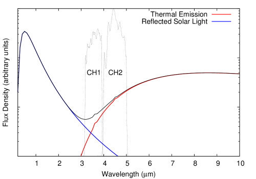
Figure 1: Spectral energy distribution of a typical arbitrary NEO with mean surface temperature of 300 K and subsolar temperature of 360 K, which are typical temperatures for objects in this program. The black line (total observed radiation) is the sum of reflected light (blue line) and thermal emission (red line). In IRAC CH1, reflected light and thermal emission can be comparable, depending on albedo and heliocentric distance, making interpretation difficult. In IRAC CH2, thermal emission dominates, and that measured flux can readily be used for thermal modeling. The IRAC bandpasses are also shown for reference.

Spitzer’s Infrared Array Camera (IRAC; Fazio et al. 2004) is the only instrument available in Spitzer’s Warm Mission, providing imaging at 3.6 and 4.5 microns (CH1 and CH2, respectively). The field of view is 5.2 arcmin. Fluxes from NEOs at CH2 are always dominated by thermal emission (Figure 1) but the ratio of reflected light to thermal emission in CH1 cannot be determined if the albedo at 3.6 microns is not known (Mainzer et al., 2011b). In our previous ExploreNEOs program (Trilling et al., 2016) we found that CH1 observations are generally not useful for thermal modeling. We therefore do not observe in CH1 in this program, saving more than 50% on our total time request.

For each potential target we predicted the thermal-infrared flux density in IRAC CH2 as a function of time. Our flux predictions were based on the absolute optical magnitude $H$, a measure of $D^{2}p_{V}$, as reported by Horizons ($D$ is diameter and $p_{V}$ is albedo). $H$ values for NEOs are of notoriously low quality and tend to be skewed to brighter magnitudes (Jurić et al., 2002; Romanishin & Tegler, 2005). To account for this, we assumed an $H$ offset ($\Delta H$) of [0.6, 0.3, 0.0] mag for [low, nominal, high] fluxes, respectively. Optical fluxes were calculated from $H+\Delta H$ together with the observing geometry. In our observation planning we assumed that asteroids are 1.4 times more reflective at 4.5 microns than in the $V$ band (Trilling et al., 2008; Harris et al., 2011; Mainzer et al., 2011b), although in our analysis pipeline we use an updated value that is derived from NEOWISE data, as described below. Thermal fluxes also depend on $p_{V}$ ($D$ is determined from $H$ and $p_{V}$) and $\eta$ (see Section 3). We assumed $p_{V}$ = [0.4, 0.2, 0.05] for [low, nominal, high] thermal fluxes. The nominal $\eta$ value was determined from the solar phase angle $\alpha$ using the linear relation given by Wolters et al. (2008), which is generally in agreement with the newer results of Mainzer et al. (2011b) and the approach used in this work (see §3.3, below); 0.3 was [added, subtracted] for [low, high] fluxes to capture the scatter in the empirical relationship derived in Wolters et al. (2008). From these parameters, we calculated the predicted thermal fluxes using the Near Earth Asteroid Thermal Model (Harris, 1998, discussed further in Section 3). We calculated [low, nominal, high] predicted fluxes in the 4.5 $\mu$m IRAC band for each day of Cycle 11. The resulting NEATM fluxes were convolved with the CH2 passband to yield “color-corrected” in-band fluxes.

After removing all dates where an NEO’s high predicted flux could saturate the detector (using saturation values from the IRAC Warm Mission Handbook), we identified a five day window centered on the peak brightness during Cycle 11. We used the minimum flux calculated for the low predicted values in this five day window to calculate our integration times and build our AORs. This five day window dictates the timing constraint that we place on the AOR. A window of this size allows good scheduling flexibility while allowing us to use the shortest possible integration times. Using the low prediction values here ensures that our SNR requirement will be met or exceeded. Our experience has shown that the ratio of observed to low predicted flux is in the range 1–10, so our conservative prediction technique is appropriate.

Our photometric requirement is SNR$\geq$15, at which point, our detailed thermal modeling shows, the flux density uncertainty becomes small compared to overall model uncertainties. We have empirically measured the Warm Spitzer CH2 sensitivity (5$\sigma$) for faint moving objects to be 2.2 $\mu$Jy in 5 hours and 1.8 $\mu$Jy in 10 hours, scaling roughly as the square root of integration time for shorter integrations (Mommert et al. 2014b). This is less sensitive than predicted by SENS-PET due to contamination from background sources that cannot be completely subtracted out in the moving frame.

Our threshold is set to integration times of $\leq$10,000 seconds (2.7 hours), which produces an AOR clock time including overheads of 3.2 hours. All sample targets have a 4.5 $\mu$m thermal-infrared flux density of 7.2 $\mu$Jy or greater. In 710.1 hours of total observation time, including all overheads, we will observe 597 NEOs. Our final sample is shown in Figures 2 and 3.

2.2 Observing strategy

We use a standard moving single target AOR, in which the telescope tracks at the appropriate moving object rates for the object, and a medium cycling dither, with only the 4.5 micron field integrating on the NEO (as we did recently for 2011 MD (Mommert et al., 2014c)). As described below, the 4.5 micron band provides the most information on the thermal emission from the NEO, whereas the 3.6 micron band can have a significant (and in general unknown) contribution from reflected light and does not significantly improve the derivation of an albedo and size. Not observing in CH1 yields significant time savings as well; since most NEOs are fainter in CH1 than in CH2 (Figure 1), observing in CH1 would more than double the needed time. Each target was assigned to one of six uniform observing templates with total frame times [120, 480, 1200, 2400, 6000, 10000] seconds. The individual frame times are 12 sec and 30 sec for the first two bins, respectively, and 100 sec for the remainder; this allows many dithers for each observation.

The frame times used for each object were chosen based on our estimate of the source flux in order to obtain the required sensitivity using the minimum total observation time. However, we have seen that occasionally the NEO is brighter than expected, possibly due to errors in the previously determined $H$ magnitude, or as in the case of Don Quixote, the result of cometary activity (Mommert et al., 2014a). We therefore use HDR mode for the 12 and 30 second frame times, which minimizes the chance of the object saturating. However, if saturation does occur, we can use a PSF-fitting technique to recover the NEO flux, as we did for Don Quixote. (Using HDR mode for the brightest targets increases the total overhead only a small amount.) For the 100 second frame times, where the objects are very likely much fainter than the saturation limit, we do not use HDR mode.

We have also checked for objects that move only slightly during the minimum observation time required to reach SNR$\geq$15. If an object moves only a small distance during the AOR, it is difficult to subtract the background field and perform accurate photometry, especially if it falls in close proximity to a bright source. We have therefore found all objects that would move less than $\sim$3 FWHMs during the observation, and added additional integrations for these sources so that the object moves sufficiently to be able to measure and subtract the background field. This has been done for approximately 50 sources, which are all relatively bright targets and have short duration AORs.

The objects in our target pool are distributed all over the sky and have an essentially uniform distribution of ecliptic longitudes (except at the Galactic plane crossings). No AOR is longer than 3.2 hours, including all overheads, and more than half the targets have AORs that are 30 minutes or less. As such, this program maximizes both total NEO yield and efficiency.

2.3 Data processing

The data processing is performed in a manner similar to our previous reductions for ExploreNEOs (Trilling et al., 2010) and our other observations of NEOs (Mommert et al., 2014b, c). The BCDs are downloaded from the Spitzer archive, and we use IRACproc/mopex in the moving object mode to mosaic the frames relative to the NEO position. For objects that are relatively bright compared to the background, and for low background fields, the outlier rejection process in the mosaicking software is sufficient to remove background objects. For fainter objects or regions of relatively high background, we often must subtract the background field before constructing the NEO mosaic. We first mosaic the data in the standard (non-moving object) mode to construct an image of the background field (the NEO is masked from the individual frames before making the background mosaic). Then we subtract the background image from each BCD, and mask any remaining strong residuals from bright background objects. We then construct the NEO mosaic from the background-subtracted BCDs. Once the NEO mosaic has been constructed, we perform aperture photometry to measure the NEO flux. We use an aperture correction derived from observations of standard stars during the Warm Mission to determine the flux.

Each mosaic is examined during the photometry process to ensure that there are no image artifacts present that will affect the photometry, and that the NEO is found in the field and not confused with background objects. The SSC produces a data delivery approximately every two weeks that will contain $\sim$14 new NEO observations from the campaign that ended two weeks prior. In most cases, we can extract fluxes and perform thermal modeling within a few days of data delivery.

3 Thermal modeling

In order to interpret the thermal-infrared flux densities measured by Spitzer, we utilize the Near-Earth Asteroid Thermal Model (NEATM, Harris, 1998). The NEATM determines the thermal-infrared flux density emitted from the surface of an asteroid by integrating the Planck function over the body’s surface temperature distribution. By combining thermal-infrared observations and optical brightness measurements ($H$), NEATM is used to fit the model flux density to the measurement in order to independently derive $D$ and $p_{V}$ of the target body. The NEATM incorporates a variable adjustment to the model surface temperature through the beaming parameter $\eta$, allowing for a correction for thermal effects of shape, spin state, thermal inertia, and surface roughness, and enabling the model and observed thermal continua to be accurately matched.

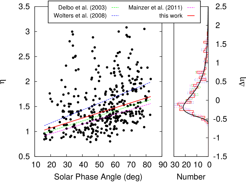
Figure 4: Left: Fitted $\eta$ values from Mainzer et al. (2011b) as a function of the average solar phase angle $\alpha$. Dashed lines represent $\eta$-$\alpha$ relations from the literature (Delbo’ et al., 2003; Wolters et al., 2008; Mainzer et al., 2011b), and the red line indicates the relation used in this work, $\eta(\alpha)=(0.01~{}{\rm deg}^{-1})\alpha+0.87$. Despite the fact that $\eta$ values scatter over the whole range from 0.6 to 3.1, a lack of high-$\alpha$ NEOs with low $\eta$, as well a general grouping of low-$\eta$ NEOs, suggest a trend between the two measures. Right: Histograms of $\eta$ residuals; $\Delta\eta$ is defined as the difference between the value of each object in the left plot and the value of the respective $\eta$ relation at the object’s $\alpha$. The histograms have been shifted in such a way that their median values coincide to improve readability. The black line is a log-normal distribution that has been fitted to the $\eta$-relation used in this work (see text).

NEATM has been applied in the successful ExploreNEOs (Trilling et al., 2010) and NEOWISE (Mainzer et al., 2011b) programs, as well as for other asteroid observations, to measure the physical properties of a large number of NEOs. In contrast, more detailed thermophysical modeling (Delbo’ et al., 2015) would require knowledge of shape and spin state, which is generally unavailable for our poorly studied targets. Even the hybrid NESTM (Wolters & Green, 2009) requires assumptions about or default values of thermal inertia and rotation period, neither of which is generally known for our targets. Additionally, Wolters & Green (2009) show that NEATM appears to overestimate diameters at phase angles larger than 45 degrees, but only by a significant amount (more than 15%) for phase angles larger than 80 degrees. Only a few percent of our targets are observed at phase angles this large. Furthemore, ultimately the Wolters & Green (2009) approach is irrelevant in our case because they considered only the cases of floating $\eta$ or fixed $\eta$. Our use of $\eta$ as a linear function of $\alpha$ will result in different behavior, and Harris et al. (2011) found no evidence in our approach for a significant phase-angle-dependent bias as a result of neglecting night-side thermal emission (their Figures 4 and 5). We therefore use NEATM, as it adequately explains our data and does not limit our analysis or interpretation.

In our (previous) ExploreNEOs program we fit the NEATM to $H$ and single-band infrared data (CH2 only, since CH1 data are heavily contaminated with reflected solar light; Mueller et al., 2011), deriving robust results: Harris et al. (2011) found that this technique leads to diameters and albedos that are accurate to within 20% and 50%, respectively, compared to previously published spacecraft, radar, and radiometric-based solutions. In this program, we apply the same modeling technique, which uses a value of $\eta$ that is not fit independently to the data but rather is based on a linear relation between $\eta$ and the solar phase angle $\alpha$, but with a more sophisticated statistical analysis of the uncertainties. In the following subsections, we provide a brief introduction to the thermal modeling pipeline and elaborate on concepts of the pipeline that differ from the ExploreNEOs approach (Trilling et al., 2010; Mueller et al., 2011).

3.1 Reflected Solar Light

The measured flux density includes both thermal emission from the asteroid’s surface and reflected solar light. The latter is generally small, but in some cases may be significant. We subtract this contribution from the measured flux densites using the method described by Mueller et al. (2011), but with an updated reflectance ratio between the optical and IR wavelengths of 1.6$\pm$0.3, which is based on measurements by WISE (Mainzer et al., 2011b), who assumed, as do we, that NEO albedos are equal at 3.6 and 4.5 microns. This albedo ratio can differ throughout the NEO population, and our error bar on this ratio captures this variance. We subtract the (estimated) reflected light contribution before calculating the color correction because reflected sunlight has a different spectral shape than asteroid thermal emission; the reflected light spectral shape is very close to the one used in the IRAC flux calibration, so the corresponding color corrections for the reflected sunlight is negligible.

In our previous program, ExploreNEOs, we corrected solar flux densities by converting from IRAC in-band flux densities to monochromatic flux densities by integrating over the model surface temperature distribution and the product of the model spectral energy distribution and the IRAC CH2 bandpass (Mueller et al., 2011), requiring an iterative approach. By contrast, in the current program, we use a different approach in which we color-correct locally emitted thermal flux density from monochromatic to IRAC CH2 in-band fluxes using the exact model temperature of that surface element at the time the Planck equation is integrated over the surface temperature distribution. In other words, we derive separate color corrections for each spot on the surface, similar to the approach used in Mainzer et al. (2011a). Using this approach, the color correction is properly iterated as part of the fitting process. The derived color corrections are in the range 5% – 20%; the only uncertainty associated comes from the ratio of reflectivity in the infrared compared to the optical (Mueller et al., 2011), and our error bars (described above) already capture our lack of knowledge of this reflectance ratio (Mueller et al., 2011). In the measured 4.5 micron flux, the reflected light fraction is between 0.01% and 29%, with a mean contribution of 1% and a median value of 0.7%. This new method produces color corrections that agree at the 1–2% level with our previous approach (Mueller et al., 2011).

3.2 $H$ magnitudes

We obtain our optical $H$ magnitudes from the ASTDyS database and improve them using statistical corrections provided by Pravec et al. (2012) over the given range of $H$ magnitudes; uncertainties are also adopted from that work. For the range of $H>20.0$, we apply a generic offset of 0.3 mag (we reduce the brightness relative to the catalog) and adopt an uncertainty of 0.3 mag, which is supported by Pravec et al. (2012), Jurić et al. (2002), and Hagen et al. (submitted). In the future we will replace ASTDyS optical data with more accurate $H$ magnitudes from ground-based surveys, where available.

3.3 Beaming Parameter Phase Relation

Because we model single-band IRAC data, we are unable to use $\eta$ as a free-floating fitting parameter. Instead, we have to make use of existing NEO thermal-infrared data to derive a robust estimate for $\eta$. As a result of asteroid surface roughness, thermal emission from the surface can be preferentially directed toward the Sun, which is referred to as infrared beaming. Energy conservation therefore requires that an observer at a high phase angle observes less thermal radiation than would be received from a smooth object, leading to a trend of increasing $\eta$ with solar phase angle $\alpha$. This trend has been quantified in the literature (Delbo’ et al., 2003; Wolters et al., 2008; Mainzer et al., 2011b) using linear relations between the parameters. In general, all of ExploreNEOs, NEOSurvey, and Warm NEOWISE must use such a derived (not fitted) $\eta$, though NEOWISE was able to fit $\eta$ directly for data obtained during their cryogenic mission, where some NEOs were detected at multiple thermal wavelengths, and both ExploreNEOs and Warm NEOWISE can fit both CH1 and CH2 thermal fluxes for very low albedo objects.

We also use a linear relation to derive the best-fit $\eta$ based on its phase angle $\alpha$, but here we take a more sophisticated approach to sample the structure and full range in the $\eta$ distribution of NEOs. Based on values of $\eta$ from NEOWISE (Mainzer et al., 2011b), which provides the largest published sample of fitted $\eta$ values, we derive a new relation. Phase angles of the observed objects are derived by querying the Minor Planet Center database for WISE observations and represent average values. Figure 4 (left) shows the $\eta$ data, the literature $\eta$-$\alpha$ relations, and our newly derived relation (see next paragraph). The NEOWISE fractional uncertainties in $\eta$ are uniformly distributed throughout this space. The high degree of scatter in $\eta$ across the whole range of phase angle is an indication of the heterogeneity in the thermal properties of NEOs and is a reminder that a simple linear relation is not sufficient to describe the variety in $\eta$. Instead, the whole range of $\eta$ values must be taken into account in a statistical approach to properly interpret thermal-infrared data. Here we derive a formalism that provides the most likely $\eta$ as a function of the phase angle, as well as an uncertainty distribution that samples the whole range of possible $\eta$ values.

From Figure 4 (left), we observe that there are no NEOs with $\eta<0.6$ or $\eta>3.1$ (0.6 is the smallest value that $\eta$ can ever take on (Mommert et al., 2012)). Furthermore, there is a clear grouping of low-$\eta$ NEOs but a lack of low-$\eta$ NEOs at high phase angles. A comparison of the $\eta$ distributions derived by Mainzer et al. (2011b) and Wolters et al. (2008) shows that the large population of NEOs with low $\eta$ is not a result of the thermal-infrared nature of the NEOWISE survey, as it is also present in the optically-selected sample by Wolters et al. (2008). For the $\eta$ relation used in this work, we adopt a slope of 0.01 deg^-1, which is in agreement with previous estimates and the slope of the lowest $\eta$ values (we show below that a slightly different slope will not affect the results). We choose the intercept of our linear relation in such a way that it divides the sample of $\eta$ values in Figure 4 (left) in two equally-sized subsamples; the probability to overestimate $\eta$ is the same as to underestimate it. Our new relation is $\eta(\alpha)=(0.01~{}{\rm deg}^{-1})\alpha+0.87$. We define the residual $\Delta\eta$ as the difference between the measured values of $\eta$ and a specific $\eta(\alpha)$. Figure 4 (right) shows that $\Delta\eta$ for the individual $\eta(\alpha)$ relations agree well with one another; despite the slightly different slopes, the shapes of the $\Delta\eta$ histograms align. We fit a log-normal distribution to the residuals using a least-squares method. The fitted distribution has parameters $\mu=0.655$ and $\sigma=0.628$, using the notation of Limpert et al. (2001). The median of the $\Delta\eta$ distribution is 0.675. The upper and lower 1$\sigma$ confidence interval of $\eta$ uncertainties spans the range from -0.3 to +0.55, relative to the nominal value of $\eta$ as derived by our $\eta(\alpha)$ relation (3$\sigma$ interval: -0.55 to +1.7). Overall, the $\eta$-$\alpha$ parameter space shown in Figure 4 is poorly sampled, and we assume that the averaged log-normal distribution shown in the right panel of Figure 4 applies across all phase angles. The data in hand do not warrant or allow any more detailed treatment of these uncertainties.

3.4 Uncertainties in derived diameter and albedo

Uncertainties in diameter and albedo are derived in a Monte Carlo approach very similar to the one described by Mueller et al. (2011). We perform 10,000 simulations with randomized parameters, including the measured flux densities that are varied based on the measured uncertainties; the absolute magnitude $H$, with Gaussian uncertainties from Pravec et al. (2012) or, for $H>20$, as a Gaussian with 1$\sigma$ uncertainties of 0.3; and the optical/IR reflectance ratio, also varied as a Gaussian. The beaming parameter $\eta$ is varied within the log-normal distribution described above. Note that occasionally values $\eta>3.1$ or $\eta<0.6$ are drawn from the distribution; these extreme values are rejected. Clipping the $\eta$ distribution affects the final results in a negligible way and is in agreement with the observations obtained by Mainzer et al. (2011b).

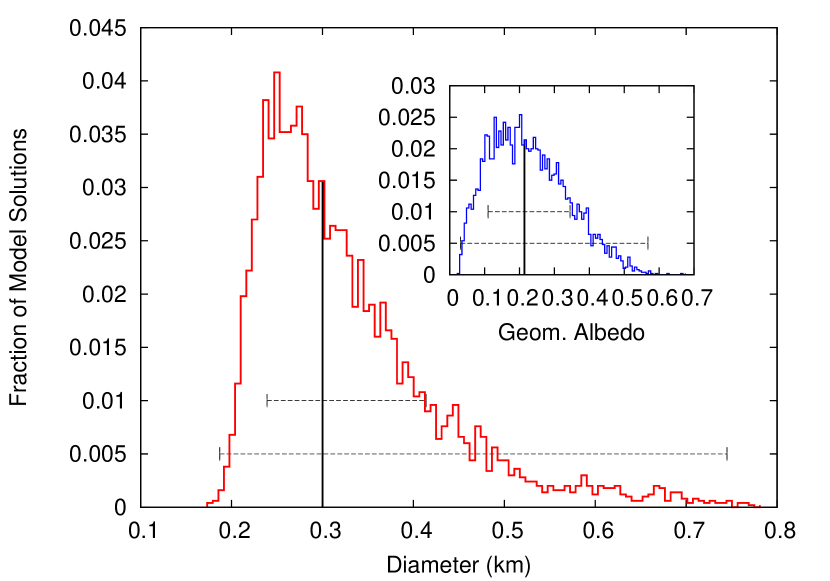
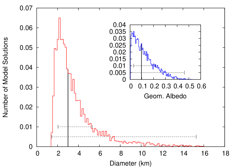
Figure 5: Probability distributions for diameter and albedo for the illustrative cases of 2012 AD3 (left) and (8567) 1996 HW1 (right). The vertical lines indicate our nominal solutions (median of the probability distributions), and 1$\sigma$ (encompassing 68.3% of the trials surrounding the median) and 3$\sigma$ (99.7% of the trials) ranges are shown with the horizontal error bars. Both diameter and albedo distributions are roughly log-normal. In this project we report both the 1$\sigma$ and 3$\sigma$ ranges for each parameter in order to capture the uncertainty distribution.

We adopt the median of the diameter and albedo distributions as our nominal solutions. We derive 1$\sigma$ and 3$\sigma$ confidence intervals as those ranges of values that bracket 68.3% and 99.7% of the values around the median, respectively. In Figure 5 we show representative cases of the diameter and albedo probability distributions that result from our thermal modeling.

The beaming parameter $\eta$ is not well constrained (Fig. 4), and drives the overall uncertainties in our model results. For the results presented here, more than 90% of the total uncertainty in diameter results from uncertainty in $\eta$. For albedo, 80%–90% of the total uncertainty is due to $\eta$ uncertainties, with uncertainties in $H$ responsible for most of the remaining uncertainty. Uncertainties in other aspects (such as emissivity) are about ten times smaller and are therefore negligible.

Finally, we make no attempt to correct for intrinsic NEO lightcurves for the targets in this program. The elapsed time of our observations spans the range 10 minutes to 3.2 hours. For the longest exposures, we might integrate over an entire asteroid rotation period, as periods of seconds to a few hours hours are common for small asteroids, in which case we derive the mean diameter from our observations. For short exposures, we could easily sample just one part of the lightcurve, in which case our solution may represent the effective spherical diameter that corresponds to a lightcurve minimum or maximum, thereby under- or overestimating the true mean diameter.

We estimate how many of our observations are affected by lightcurve effects with a Monte Carlo approach. Taking into account the measured lightcurve amplitude distribution of known NEOs (Warner et al., 2009), we randomly sample sine curves with different amplitudes to simulate the offset from the lightcurve-averaged thermal flux of the target in our observations and produce diameter and albedo solutions that correspond to this instantaneous sampling. We find that 3–6% of all trials have diameter discrepancies greater than our quoted diameter uncertainty of 40%. Hence, we expect the same fraction of our targets to have diameters affected by lightcurve-induced discrepancies greater than 1$\sigma$. For our albedo solutions, 5–9% of trials have solutions greater than our quoted albedo uncertainty of 70%. If we smooth the lightcurve over 20% of its period (which is a more realistic approximation of the situation), we find that fewer than 5% of our diameters and fewer than 9% of our albedos are affected by this lightcurve sampling.

Derived albedos that are (much) greater than around 0.5 are suspicious, as such values are rarely seen for asteroids for which albedos have been reliably measured (for radar or spacecraft measurements, for example, as opposed to radiometric approaches), and are at odds with expected surface compositions. The most likely explanations for such high albedos are $H$ magnitudes that are significantly incorrect and/or (optical or thermal) lightcurve amplitudes and periods that produce a high albedo solution. In both cases, additional ground-based photometry can allow us to correct our albedo solution. We have initiated such a program using a range of ground-based telescopes, and in a future paper we will report revised optical magnitudes and/or lightcurves for these high albedo objects, along with re-calculated albedos. (Note that poor $H$ values and/or lightcurves could also produce anomalously low albedos, which may be harder to identify. We will carry out ground-based observations of the objects for which we find the lowest albedos to determine if a correction is also needed for those objects.)

3.5 Validation of our approach

A small number of our targets will be observed by NEOWISE — it is impossible to calculate which targets will overlap in the future, since the NEOWISE SPICE kernel (orbit) is only published a few months ahead — and we will use those targets as cross-checks. Furthermore, there are more than 100 NEOs that have been observed by NEOWISE that were also observed in our ExploreNEOs program (Trilling et al., 2016). For these common objects, we use our updated thermal model pipeline and used only CH2 data (as if the ExploreNEOs data were obtained in this NEOSurvey program) to rederive the diameter and albedo from our ExploreNEOs measurements, and compare these to the published NEOWISE diameters and albedos (Mainzer et al., 2011b). The mean ratio of ExploreNEOs values to NEOWISE values for [diameter, albedo] is [0.9, 1.28]. The median value in this ratio of ExploreNEOs values to NEOWISE values for [diameter, albedo] is [0.9, 1.02]. This overall agreement, based on independent data measurements and modeling, is quite good, although we caution that for any individual object significantly different solutions may exist. For diameter, 70% of the newly modeled ExploreNEOs targets have 1$\sigma$ error bars that overlap with NEOWISE values; 98% of the targets agree at 3$\sigma$. For albedo, 66% of the newly modeled ExploreNEOs targets have 1$\sigma$ error bars that overlap with NEOWISE values; 98% of the targets agree at 3$\sigma$. This suggests that both the errors are largely random, and that our error bar estimations are appropriate. The largest deviation is in albedo, where uncertainties in $H$ magnitude typically introduce large errors, and where the two approaches frequently use somewhat different $H$ magnitudes for their modeling. In the future we will carry out a more comprehensive comparison, considering targets that overlap with both ExploreNEOs and NEOSurvey, and using common $H$ values for the thermal modeling of the different thermal measurements.

4 First results from NEOSurvey

We report here results for the first 80 NEOs observed in this program. These NEOs were observed in February and March, 2015. Table 1 gives the geometries, measured fluxes, and derived diameter and albedo results for these targets. As described above, the probability distributions for the results are asymmetric and non-Gaussian. We therefore provide 1$\sigma$ and 3$\sigma$ upper and lower diameter and albedo values for each target.

We introduce here nearearthobjects.nau.edu, a publicly accessible webpage where all information from this program is posted. Table 2 lists the properties for each observed object that are available in our online database, where we list complete observing circumstances and modeling results. The observing cadence for this program is roughly one target per day. Data is made available to us at a biweekly cadence. It takes us typically 1–2 days from receiving the data to producing model results. Therefore, our online database grows continuously, in roughly two week intervals, over the duration of this program. The latest version of our results will always be available on that webpage. Because of the Monte Carlo nature of our modeling solutions, the values in this online table can very slightly with time, but all such changes are insignificant compared to the size of the error bars. The database ultimately will also host all ExploreNEOs data, with results derived from the latest version of our pipeline. Relevant publications will also be posted at that webpage.

5 Future work

As our survey proceeds and our catalog grows, a number of science investigations will be enabled, including the following. (1) Our sample is optically selected, so any study of the properties of the entire NEO population requires rigorous debiasing, which is a signficant challenge. Using debiasing approaches that we have developed (Trilling et al., 2016; Mommert et al., 2015) and continue to enhance, we will measure the size distribution of NEOs down to 100 meters. We will observe nearly 200 NEOs smaller than 200 meters ($H>20$; Figure 3). This will allow us to calculate an independent measurement of the NEO size distribution, one that is derived from a sample size at 100 meters that is more than three times as large as all the previous thermal infrared surveys combined. (2) By applying those same debiasing approaches to the combination of NEOSurvey, ExploreNEOs, and NEOWISE data we will derive the distribution of albedos and compositions as a function of size. (3) We will search for “dead comets” — bodies that dynamically, and presumably compositionally, are of cometary origin, but typically exhibit no cometary activity. Our target sample includes 32 potential dead comets, based on their low, comet-like Tisserand parameters, $T_{J}\leq 3.0$. Our albedo measurements for all these objects may provide further evidence for their cometary nature (cometary albedos are extraordinarily low), as it did for the NEO Don Quixote (Mommert et al., 2014a). (4) There are 109 targets in our sample that obey the usual “mission accessible” definition of $\Delta v<7$ km/s (and six targets that have $\Delta v<5$ km/s). We will measure diameters and albedos for these NEOs and, together with historical temperature modeling as in Mueller et al. (2011), identify the most primitive objects — and therefore most interesting for mission planning — in our sample. (5) By determining the albedos of NEOs, we can measure the compositions of small bodies in the various source regions. These results can be compared to models from Bottke et al. (2002) and recent work by Granvik et al. (2014) to make connections among meteorite, NEOs, and parent asteroids or asteroid families in the main belt, thereby providing geologic, mineralogic, and Solar System context to the objects studied in our laboratories and by our space missions.

The preceding list is not meant to be exhaustive, as many other investigations will be possible, both by members of the survey team and other researchers. The ultimate result will be a catalog of some 2000 NEO properties, derived from the union of NEOWISE, ExploreNEOs, Akari, and NEOSurvey results. This will represent nearly 20% of all known NEOs in late 2016 when our NEOSurvey concludes.

Figure 2: Maximum low CH2 flux density predictions as a function of $H$ magnitude. The dots show all NEOs accessible with Spitzer in Cycle 11. Dashed lines indicate the $15\sigma$ sensitivities for the NEOWISE survey and this program. The sensitivity limit for NEOWISE W2 (890 $\mu$Jy) is derived from flux densities tabulated in Mainzer et al. (2014b) and the flux calibration information in Wright et al. (2010). We set our integration cutoff to be 10,000 seconds, and observe all targets whose peak brightnesses are greater than 7.2 $\mu$Jy, as indicated: all dots above the dotted line marked “this program.” There are many small NEOs in this sample, with some 200 targets smaller than 200 meters ($H>20$). The vast majority of our targets are too faint to be observed by NEOWISE. Objects above the NEOWISE flux limit as seen by Spitzer may not be bright enough to be detected by NEOWISE when in the NEOWISE field of view, and the reverse: some objects that are below the NEOWISE faint limit as seen by Spitzer may be brighter when they are observed by NEOWISE. Therefore, a small number of NEOs will be observed by both Spitzer and NEOWISE, which allows for a cross-check of our mutual results.

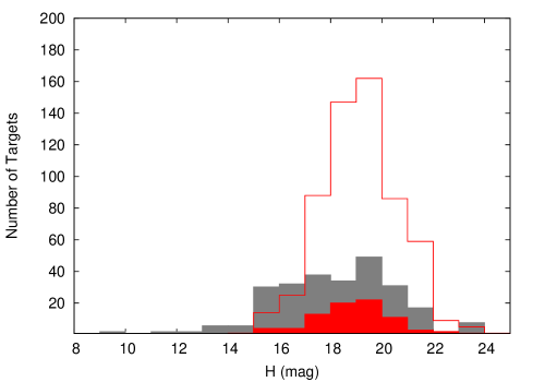
Figure 3: Distribution of $H$ magnitudes for targets to be observed in this sample (thin solid red line and unshaded histogram) and by NEOWISE during Spitzer’s Cycle 11 (shaded gray region). The 80 targets observed to date in this program are shown as the shaded red histogram. Because the NEOWISE SPICE kernel (orbit) is only published a few months ahead, it is impossible to calculate exactly which NEOs will be observed by NEOWISE during Spitzer’s Cycle 11, but we can closely estimate the $H$ distribution by scaling the NEOWISE yield since reactivation to the duration of Spitzer’s Cycle 11. A diameter of 100 meters corresponds roughly to $H$ of 22.5. At $H>20$, this project contains more than three times as many targets as NEOWISE and ExploreNEOs combined.

Table 1: Target information and results

Target	r	$\Delta$	phase	$H$	$\Delta H$	F4.5	$\eta$	$D$	$D~{}(3\sigma)$	$p_{V}$	$p_{V}~{}(3\sigma)$
	(AU)	(AU)	(deg)	(mag)	(mag)	($\mu$Jy)		(m)	(m)
8567 (1996 HW1)	2.07	1.90	29.3	15.76	0.22	91$\pm$9	1.14	2900 (-900/+2400)	1500—12100	0.10 (-0.07/+0.13)	0.00—0.42
35396 (1997 XF11)	1.36	0.59	43.7	17.11	0.22	519$\pm$22	1.29	940 (-220/+480)	380—1930	0.29 (-0.16/+0.21)	0.03—0.60
162117 (1998 SD15)	1.25	0.46	50.2	19.41	0.22	147$\pm$11	1.34	350 (-80/+160)	140—660	0.25 (-0.14/+0.18)	0.02—0.49
208023 (1999 AQ10)	1.08	0.14	59.3	20.60	0.30	365$\pm$18	1.44	148 (-26/+52)	52—201	0.46 (-0.22/+0.25)	0.06—0.69
(2004 TP1)	1.03	0.17	81.8	20.90	0.30	315$\pm$16	1.65	207 (-38/+74)	70—253	0.18 (-0.09/+0.11)	0.03—0.36
390929 (2005 GP21)	1.04	0.17	76.5	20.80	0.30	238$\pm$14	1.60	179 (-32/+62)	62—222	0.26 (-0.12/+0.15)	0.04—0.47
434734 (2006 FX)	1.05	0.36	75.4	20.30	0.30	66$\pm$8	1.59	198 (-35/+69)	72—242	0.34 (-0.16/+0.19)	0.06—0.55
(2008 SU1)	1.19	0.63	58.6	19.51	0.22	113$\pm$10	1.42	410 (-90/+190)	170—720	0.16 (-0.09/+0.11)	0.02—0.36
(2008 UF7)	1.41	0.62	40.7	19.41	0.22	54$\pm$7	1.25	330 (-80/+170)	140—740	0.28 (-0.17/+0.22)	0.02—0.65
(2010 XP51)	1.24	0.39	48.1	18.93	0.22	2119$\pm$42	1.32	970 (-240/+510)	430—2070	0.05 (-0.03/+0.04)	0.00—0.14
(2011 SM68)	1.09	0.50	68.3	19.89	0.22	57$\pm$7	1.51	241 (-44/+90)	86—338	0.33 (-0.16/+0.18)	0.05—0.51
(2011 WS2)	1.52	1.22	41.8	17.59	0.22	149$\pm$11	1.26	1240 (-340/+750)	590—3360	0.10 (-0.06/+0.10)	0.01—0.33
(2012 AD3)	1.12	0.47	64.7	19.89	0.22	96$\pm$9	1.48	290 (-60/+120)	110—450	0.24 (-0.12/+0.14)	0.03—0.43
14827 Hypnos (1986 JK)	1.32	0.93	50.2	18.65	0.22	65$\pm$7	1.35	520 (-120/+260)	220—1030	0.22 (-0.12/+0.17)	0.02—0.50
4487 Pocahontas (1987 UA)	1.22	0.66	56.4	17.68	0.22	789$\pm$26	1.41	1150 (-270/+570)	480—2110	0.11 (-0.06/+0.09)	0.01—0.29
5332 Davidaguilar (1990 DA)	1.64	1.32	38.2	15.09	0.22	634$\pm$24	1.22	3300 (-900/+2000)	1500—9200	0.15 (-0.10/+0.14)	0.01—0.44
8034 Akka (1992 LR)	1.41	0.78	44.8	18.16	0.22	78$\pm$8	1.29	540 (-120/+260)	220—1170	0.33 (-0.18/+0.23)	0.03—0.63
32906 (1994 RH)	1.33	0.66	48.2	16.15	0.22	2266$\pm$43	1.32	2080 (-510/+1100)	880—4510	0.14 (-0.08/+0.11)	0.01—0.36
(1998 WP7)	1.07	0.35	71.6	20.18	0.22	133$\pm$11	1.55	256 (-49/+93)	93—346	0.23 (-0.11/+0.13)	0.04—0.38
137078 (1998 XZ4)	1.40	0.82	46.1	16.63	0.22	274$\pm$16	1.30	1070 (-230/+510)	430—2140	0.34 (-0.19/+0.23)	0.03—0.61
53409 (1999 LU7)	1.19	0.54	58.5	19.03	0.22	232$\pm$14	1.42	510 (-110/+240)	200—870	0.17 (-0.09/+0.12)	0.02—0.35
102873 (1999 WK11)	1.58	1.00	38.6	17.78	0.22	32$\pm$5	1.23	570 (-130/+290)	240—1430	0.43 (-0.25/+0.31)	0.03—0.85
178601 (2000 CG59)	1.48	1.21	42.8	17.88	0.22	90$\pm$9	1.26	920 (-240/+530)	420—2340	0.15 (-0.09/+0.13)	0.01—0.41
159495 (2000 UV16)	1.37	0.67	44.9	17.40	0.22	329$\pm$17	1.29	870 (-200/+440)	350—1920	0.26 (-0.15/+0.19)	0.02—0.53
162723 (2000 VM2)	1.21	0.35	48.2	17.68	0.22	812$\pm$27	1.32	600 (-120/+250)	210—1040	0.42 (-0.21/+0.25)	0.04—0.65
162741 (2000 WG6)	1.27	0.44	46.1	17.78	0.22	17336$\pm$191	1.30	3100 (-800/+1700)	1500—7100	0.01 (-0.01/+0.01)	0.00—0.04
(2000 WP19)	1.04	0.06	68.1	22.70	0.30	2827$\pm$48	1.52	176 (-37/+73)	68—261	0.05 (-0.02/+0.04)	0.01—0.13
68346 (2001 KZ66)	1.35	0.95	48.9	17.11	0.22	219$\pm$14	1.32	1010 (-230/+520)	400—2120	0.25 (-0.14/+0.17)	0.03—0.51
283460 (2001 PD1)	1.21	0.75	56.5	18.55	0.22	230$\pm$14	1.40	700 (-160/+320)	290—1300	0.14 (-0.07/+0.10)	0.02—0.30
317685 (2003 NO4)	1.53	0.81	37.5	18.45	0.22	74$\pm$8	1.21	570 (-150/+320)	260—1550	0.22 (-0.13/+0.19)	0.01—0.57
143992 (2004 AF)	1.33	0.94	49.6	16.43	0.22	1064$\pm$30	1.33	2050 (-510/+1100)	880—4440	0.11 (-0.07/+0.09)	0.01—0.28
267940 (2004 EM20)	1.15	0.33	57.4	20.50	0.30	61$\pm$7	1.42	160 (-30/+62)	58—245	0.44 (-0.21/+0.25)	0.06—0.72
154715 (2004 LB6)	1.14	0.60	62.7	18.74	0.22	129$\pm$10	1.47	430 (-80/+170)	150—650	0.30 (-0.15/+0.18)	0.04—0.50
(2004 QD14)	1.04	0.12	73.9	20.90	0.30	352$\pm$17	1.57	143 (-24/+49)	47—174	0.37 (-0.18/+0.20)	0.05—0.58
318160 (2004 QZ2)	1.14	0.47	62.4	18.36	0.22	256$\pm$15	1.46	490 (-90/+190)	170—730	0.33 (-0.16/+0.19)	0.04—0.53
(2005 XY)	1.35	0.76	48.5	19.13	0.22	97$\pm$9	1.33	520 (-130/+270)	230—1140	0.15 (-0.08/+0.12)	0.02—0.38
(2006 VD13)	1.09	0.31	68.0	19.32	0.22	360$\pm$18	1.53	370 (-70/+140)	130—500	0.24 (-0.12/+0.14)	0.03—0.41
(2006 VD2)	1.10	0.41	67.6	19.51	0.22	314$\pm$16	1.51	430 (-90/+180)	170—640	0.15 (-0.08/+0.09)	0.02—0.28
375103 (2007 TD71)	1.30	0.70	50.7	18.74	0.22	91$\pm$9	1.34	460 (-100/+220)	190—910	0.26 (-0.15/+0.18)	0.02—0.53
(2008 SQ)	1.25	0.51	52.1	19.80	0.22	86$\pm$9	1.36	300 (-70/+140)	120—580	0.24 (-0.13/+0.17)	0.02—0.49
(2010 KU10)	1.15	0.40	60.5	19.80	0.22	236$\pm$14	1.44	360 (-80/+160)	140—620	0.16 (-0.08/+0.11)	0.02—0.34
(2010 TJ7)	1.17	0.41	58.4	19.99	0.22	185$\pm$13	1.42	330 (-70/+150)	130—570	0.17 (-0.09/+0.11)	0.02—0.34
(2010 VN65)	1.11	0.40	66.1	20.40	0.30	57$\pm$7	1.50	193 (-37/+72)	70—281	0.32 (-0.16/+0.20)	0.04—0.65
(2011 HR)	1.25	0.47	50.8	20.09	0.22	42$\pm$6	1.35	202 (-40/+88)	77—366	0.40 (-0.21/+0.24)	0.04—0.70
(2012 AS10)	1.56	1.20	40.5	17.59	0.22	44$\pm$6	1.25	750 (-180/+420)	330—1900	0.29 (-0.17/+0.23)	0.02—0.64
(2014 MQ18)	1.57	0.92	38.1	16.15	0.22	4023$\pm$60	1.22	4800 (-1400/+3200)	2400—14000	0.03 (-0.02/+0.03)	0.00—0.10
152560 (1991 BN)	1.33	0.55	43.6	19.32	0.22	62$\pm$7	1.29	290 (-60/+140)	120—570	0.38 (-0.21/+0.25)	0.04—0.71
337053 (1996 XW1)	1.10	0.44	67.1	19.22	0.22	105$\pm$9	1.51	296 (-52/+106)	100—393	0.41 (-0.20/+0.21)	0.06—0.59
312956 (1997 CZ3)	1.04	0.17	74.8	19.80	0.22	3386$\pm$54	1.59	580 (-120/+230)	220—780	0.06 (-0.03/+0.04)	0.01—0.13
53430 (1999 TY16)	1.53	1.02	41.0	17.01	0.22	348$\pm$17	1.25	1580 (-430/+950)	740—4220	0.11 (-0.07/+0.10)	0.01—0.33
331509 (1999 YA)	1.41	0.66	41.1	18.45	0.22	104$\pm$9	1.25	490 (-110/+260)	200—1170	0.31 (-0.18/+0.22)	0.03—0.64
68063 (2000 YJ66)	2.18	1.51	24.1	15.86	0.22	61$\pm$7	1.10	2100 (-700/+1700)	1100—9800	0.18 (-0.13/+0.22)	0.01—0.63
159533 (2001 HH31)	1.75	1.08	31.9	17.97	0.22	37$\pm$6	1.17	710 (-200/+460)	350—2390	0.22 (-0.14/+0.22)	0.01—0.64
286079 (2001 TW1)	1.32	0.52	44.5	19.41	0.22	64$\pm$7	1.28	280 (-60/+130)	110—580	0.39 (-0.21/+0.25)	0.04—0.70
(2002 VO85)	1.11	0.19	53.0	21.80	0.30	149$\pm$11	1.37	113 (-24/+50)	45—189	0.26 (-0.14/+0.19)	0.03—0.59
(2002 VV17)	1.08	0.15	60.4	20.18	0.22	803$\pm$26	1.44	229 (-43/+91)	80—332	0.28 (-0.14/+0.16)	0.04—0.49
280244 (2002 WP11)	1.58	0.82	34.4	18.45	0.22	59$\pm$7	1.19	540 (-140/+320)	240—1510	0.25 (-0.16/+0.22)	0.01—0.64
(2004 JR)	1.22	0.76	56.1	19.03	0.22	234$\pm$14	1.40	710 (-170/+340)	300—1360	0.09 (-0.05/+0.07)	0.01—0.22
351508 (2005 RN33)	1.37	0.55	40.4	19.89	0.22	47$\pm$6	1.25	250 (-60/+130)	110—580	0.30 (-0.17/+0.22)	0.02—0.63
(2005 VC2)	1.23	0.40	49.3	18.07	0.22	29171$\pm$204	1.33	3600 (-900/+1900)	1600—7400	0.01 (-0.00/+0.01)	0.00—0.03
(2005 XT77)	1.05	0.13	69.1	21.20	0.30	177$\pm$12	1.52	112 (-19/+38)	37—137	0.46 (-0.21/+0.23)	0.07—0.66
417949 (2007 TB23)	1.40	0.62	40.3	19.03	0.22	37$\pm$6	1.24	290 (-60/+130)	110—630	0.51 (-0.28/+0.31)	0.04—0.80
(2007 WB5)	1.14	0.49	62.8	19.41	0.22	93$\pm$9	1.46	300 (-60/+120)	110—460	0.33 (-0.16/+0.19)	0.05—0.53
(2009 FF19)	1.03	0.05	72.9	21.70	0.30	1938$\pm$41	1.56	136 (-26/+49)	47—176	0.20 (-0.10/+0.13)	0.03—0.38
(2009 KN4)	1.09	0.52	67.7	18.55	0.22	365$\pm$18	1.51	590 (-120/+240)	210—870	0.19 (-0.10/+0.12)	0.03—0.35
407338 (2010 RQ30)	1.18	0.29	49.1	18.55	0.22	1228$\pm$32	1.33	530 (-120/+250)	210—990	0.23 (-0.13/+0.16)	0.02—0.46
(2010 VF1)	1.14	0.28	57.0	20.70	0.30	241$\pm$14	1.40	229 (-49/+104)	90—388	0.17 (-0.09/+0.13)	0.01—0.42
436761 (2012 DN)	1.31	0.85	50.8	18.55	0.22	1015$\pm$29	1.35	1730 (-450/+950)	790—3730	0.02 (-0.01/+0.02)	0.00—0.07
(2012 RG3)	1.07	0.24	69.9	18.26	0.22	1332$\pm$33	1.54	550 (-100/+200)	180—720	0.29 (-0.14/+0.16)	0.05—0.46
(2012 UA34)	1.09	0.38	68.4	19.89	0.22	71$\pm$8	1.53	214 (-37/+74)	71—268	0.43 (-0.19/+0.21)	0.07—0.59
(2013 QK48)	1.22	0.52	55.2	18.65	0.22	242$\pm$14	1.38	510 (-110/+230)	200—910	0.24 (-0.12/+0.15)	0.03—0.44
(2014 NF64)	1.29	0.83	51.8	18.65	0.22	146$\pm$11	1.35	660 (-160/+340)	280—1330	0.14 (-0.08/+0.11)	0.01—0.34
(2014 OL339)	1.05	0.12	67.7	23.00	0.30	71$\pm$8	1.51	58 (-11/+22)	21—83	0.33 (-0.16/+0.19)	0.04—0.57
(2014 QW296)	1.55	0.81	36.0	19.13	0.22	63$\pm$7	1.20	520 (-150/+320)	250—1470	0.15 (-0.09/+0.14)	0.01—0.48
136618 (1994 CN2)	1.12	0.60	63.5	17.11	0.22	339$\pm$18	1.48	730 (-130/+270)	240—970	0.47 (-0.22/+0.23)	0.07—0.61
137427 (1999 TF211)	2.27	2.12	26.3	15.47	0.22	46$\pm$6	1.11	2900 (-1000/+2500)	1600—13500	0.14 (-0.10/+0.18)	0.01—0.54
54509 YORP (2000 PH5)	1.04	0.05	58.5	22.90	0.30	282$\pm$16	1.42	47 (-8/+15)	16—60	0.56 (-0.25/+0.27)	0.09—0.71
228368 (2000 WK10)	1.12	0.52	64.2	18.65	0.22	206$\pm$13	1.48	470 (-90/+180)	170—680	0.28 (-0.14/+0.16)	0.04—0.47
(2002 AQ2)	1.09	0.42	68.5	18.93	0.22	364$\pm$18	1.52	490 (-100/+190)	170—690	0.20 (-0.10/+0.12)	0.03—0.37
(2012 GG1)	1.18	0.71	58.6	18.93	0.22	219$\pm$14	1.43	620 (-140/+270)	250—1080	0.12 (-0.06/+0.09)	0.01—0.28

Note. — The columns are as follows: target name; heliocentric and Spitzer-centric distances; phase angle of observations (in Spitzer-centric reference frame); corrected $H$ magnitude and applied uncertainty (see Section 3.2); in-band measured fluxes at 4.5 microns, where the uncertainties do not include the 5% calibration uncertainty; nominal $\eta$ value applied in the modeling, as calculated from phase angle (see description in text); and derived albedos and diameters, where 1$\sigma$ uncertainties are given in parentheses and 3$\sigma$ ranges are listed. Note that the in-band fluxes listed here must be color-corrected as described in the text in order to carry out the thermal modeling and derive diameters and albedos. In some cases the albedo errors formally include zero, which should be interpreted as indicating that the minimum albedo is a small non-zero number. Further information about the observations and model results (including AORKey, which is a unique Spitzer identifier for each observation; date and time of the observations; details of the exposure times; and uncertainties in $\eta$) is available from our online database; see Table 2 for more details.

Table 2: Properties listed in our online table

Object number	Object name	Object designation
Semi-major axis	Eccentricity	Inclination
Long. asc. node $\Omega$	Arg. perihelion $\omega$	Orbital period
Observed RA	Observed Dec	3$\sigma$ RA Uncert.	3$\sigma$ Dec Uncert.
V magnitude	Heliocentric distance	Spitzer-centric distance
Phase angle	Solar elong. angle	Galactic latitude	Galactic longitude
Date of observation	JD of observation	AORKey
Frame time	Total integration time	Elapsed time	Notes about the observation or data quality
CH2 flux	CH2 error	CH2 SNR
$H$ magnitude	Uncertainty on $H$ magnitude	G (slope parameter)
$\eta$	$\eta$: $\pm$1$\sigma$	$\eta$: $\pm$3$\sigma$
Diameter	Diameter: $\pm$1$\sigma$	Diameter: $\pm$3$\sigma$
Albedo	Albedo: $\pm$1$\sigma$	Albedo: $\pm$3$\sigma$

Note. — These quantities and their units are fully defined at nearearthobjects.nau.edu .

References

- Abe et al. (2012) Abe, M., Yoshikawa, M., Sugita, S. et al. 2012, Proc. of Asteroids, Comets, Meteors, #6137
- Abell et al. (2016) Abell, P.A., Mazanek, D.D., Reeves, D.M. et al. 2016, LPSC 47, 2217
- Barbee et al. (2013) Barbee, B.W., Wie, B., Steiner, M., & Getzandanner, K. 2013, Planetary Defense Conference 2013, IAA-PDC13-04-07.
- Bottke et al. (2002) Bottke, W. F., Morbidelli, A., Jedicke, R., et al. 2002, Icarus, 156, 399
- Brown et al. (2013) Brown, P., Assink, J. D., Astiz, L., et al. 2013, Nature, 503, 238
- Delbo’ et al. (2003) Delbo’, M., Harris, A. W., Binzel, R. P., et al. 2003, Icarus, 166, 116
- Delbo’ et al. (2015) Delbo’, M., Mueller, M., Emery, J. P., et al. 2015, in Asteroids IV, eds. P. Michel et al. (Univ. of Arizona Press, Tucson), 107
- Dermawan et al. (2011) Dermawan, B., Nakamura, T., & Yoshida, F. 2011, PASJ, 63, 555
- Fazio et al. (2004) Fazio, G., Hora, J., Allen, L., et al. 2004, ApJS, 154, 10
- Fujiwara et al. (2006) Fujiwara, A., Kawaguchi, J., Yeomans, D.K. et al. 2006, Science, 312, 1330
- Granvik et al. (2014) Granvik, M., Morbidelli, A., Jedicke, R., et al. 2014, in Asteroids, Comets, Meteors 2014, eds. Muinonen et al. (http://www.helsinki.fi/acm2014/pdf-material/ACM2014.pdf)
- Hagen et al. (submitted) Hagen, A., Trilling, D. E., Penprese, B. E., et al., 2016, AJ, submitted
- Harris (1998) Harris, A. W. 1998, Icarus, 131, 291
- Harris & Lagerros (2002) Harris, A. & Lagerros, J. S. V. 2002, in Asteroids III, eds. Bottke et al. (Tucson: U. Arizona Press), 205
- Harris et al. (2011) Harris, A. W. Mommert, M., Hora, J. L., et al. 2011, AJ, 141, 75
- Hasegawa et al. (2013) Hasegawa, S., Müller, T. G., Kuroda, D., et al. 2013, PASJ, 65, 34
- Ji et al. (2016) Ji, J., Jiang, Y., Zhao, Y. et al. 2016, Proc. of the IAU, 318, 144
- Jurić et al. (2002) Jurić, M., Ivezić, Ž., Lupton, R. H., et al. 2002, AJ, 124, 1776
- Lauretta et al. (2015) Lauretta, D.S., Bartels, A.E., Barucci, M.A. et al. 2015, M&PS, 50, 834
- Limpert et al. (2001) Limpert, E., Stahel, A. E., Abbt, M. 2001, BioScience, 51, 5
- Mainzer et al. (2011a) Mainzer et al. 2011a, ApJ, 741, 90
- Mainzer et al. (2011b) Mainzer, A., Grav, T., Bauer, J., et al. 2011b, ApJ, 743, 156
- Mainzer et al. (2012) Mainzer, A., Grav, T., Masiero, J., et al. 2012, ApJ, 752, 110
- Mainzer et al. (2014) Mainzer, A., Bauer, J., Grav, T., et al. 2014a, ApJ, 784, 110
- Mainzer et al. (2015) Mainzer, A., Usui, F., & Trilling, D. 2015, in Asteroids IV, eds. P. Michel et al. (Univ. of Arizona Press, Tucson), 89
- Marengo et al. (2009) Marengo, M., Stapelfeldt, K. R., Werner, M. W., et al. 2009, ApJ, 700, 1647
- Masiero et al. (2009) Masiero, J., Jedicke, R., Ďurech, J., et al. 2009, Icarus, 204, 145
- Mommert et al. (2012) Mommert, M., Harris, A. W., Kiss, C., et al. 2012, A&A, 541, A93
- Mommert et al. (2014a) Mommert, M. Hora, J. L., Harris, A. W., et al. 2014a, ApJ, 781, 25
- Mommert et al. (2014b) Mommert, M., Hora, J. L., Farnocchia, D., et al. 2014b, ApJ, 786, 148
- Mommert et al. (2014c) Mommert, M., Farnocchia, D., Hora, J. L., et al. 2014c, ApJL, 789, 22
- Mommert et al. (2015) Mommert, M., Harris, A. W., Mueller, M., et al. 2015, AJ, submitted
- Mueller et al. (2007) Mueller, M., Harris, A. W., & Fitzsimmons, A. 2007, Icarus, 187, 611
- Mueller et al. (2011) Mueller, M., Delbo’, M., Hora, J. L., et al. 2011, AJ, 141, 109
- Nugent et al. (2015) Nugent, C.R., Mainzer, A., Masiero, J., et al. 2015, ApJ, 814, 117
- Popova et al. (2013) Popova, O.P., Jenniskens, P., Emel’yanenko, V. et al. 2013, Science, 342, 1069
- Pravec et al. (2012) Pravec, P., Harris, A.W., Kušnirák, P., et al. 2012, Icarus, 221, 365
- Rivkin et al. (2005) Rivkin, A.S., Binzel, R.P., & Bus, S.J. 2005, Icarus, 175, 175
- Romanishin & Tegler (2005) Romanishin, W. & Tegler, S. C. 2005, Icarus, 179, 523
- Thomas et al. (2011) Thomas, C. A., Trilling, D. E., Emery, J. P., et al. 2011, AJ, 142, 85
- Trilling & Bernstein (2006) Trilling, D. E. & Bernstein, G. M. 2006, AJ, 131, 1149
- Trilling et al. (2008) Trilling, D. E., Mueller, M., Hora, J. L., et al. 2008, ApJL, 683, 199
- Trilling et al. (2010) Trilling, D. E., Mueller, M., Hora, J. L., et al. 2010, AJ, 140, 770
- Trilling et al. (2016) Trilling, D. E., Mommert, M., Mueller, M., et al. 2016, AJ, submitted
- Usui et al. (2011) Usui, F., Kasuga, T., Hasegawa, S., et al. 2011, PASJ, 63, 1117
- Vernazza et al. (2008) Vernazza, P., Binzel, R. P., Thomas, C. A., et al. 2008, Nature, 454, 858
- Veverka et al. (2001) Veverka, J., Thomas, P.C., Robinson, M. et al. 2001, Science, 292, 484
- Warner et al. (2009) Warner, B. D., Harris, A. W., & Pravec, P. 2009, Icarus, 202, 134
- Wolters et al. (2008) Wolters, S. D., Green, S. F., McBride, N., & Davies, J. K. 2008, Icarus, 193, 535
- Wolters & Green (2009) Wolters, S. D. & Green, S. F. 2009, MNRAS, 400, 204
- Wright et al. (2010) Wright, E. L., Eisenhardt, P., Mainzer, A. K., et al. 2010, AJ, 140, 1868