Real algebraic knots and links of small degree

Abstract.

The paper gives a topological as well as rigid isotopy classification of smooth irreducible algebraic curves in the real projective 3-space for the case when the degree of the curve is at most six and its genus is at most one.

The subject of this paper is the problem of topological classification of smooth algebraic curves in ${\mathbb{R}}{\mathbb{P}}^{3}$ when their genus and degree are fixed. The ${\mathbb{R}}{\mathbb{P}}^{2}$ counterpart of this problem had originated in the celebrated work [4] of Harnack, was popularized by Hilbert in his famous list of problems [5] and consequently it was well-studied over the last century. In the same time the corresponding topological classification in ${\mathbb{R}}{\mathbb{P}}^{3}$ remains relatively unstudied. We note that such classification is straightforward in the case when the degree is $4$ or less as all relevant curves are contained either in a plane or in a quadric surface. The classification in the case of degree 5 and genus 0 was obtained by Johan Bjorklund [1]. Our paper continues this work by providing the classification in the case of degree 5 and genus 1 as well as for degree 6 and genus $\leq 1$.

1. Planar knots

Let $\mathbb{R}K\subset{\mathbb{R}}{\mathbb{P}}^{3}$ be a smooth irreducible real algebraic curve of degree $d$ and genus $g$ consisting of $l$ connected components. This means that $\mathbb{R}K\subset{\mathbb{R}}{\mathbb{P}}^{3}$ is given by a system of homogeneous real polynomial equations in four variables so that the locus $K\subset{\mathbb{P}}^{3}$ of complex solutions of the same system of equations is an irreducible complex curve of genus $g$ smoothly embedded to ${\mathbb{P}}^{3}$ and homologous to $d[{\mathbb{P}}^{1}]\in H_{2}({\mathbb{P}}^{3})=\mathbb{Z}$. Recall that by the Harnack inequality we have $l\leq g+1$. We assume that $\mathbb{R}K$ is non-empty, i.e. that $l\geq 1$.

Proposition 1.

We have $g\leq\frac{(d-1)(d-2)}{2}$. If $g=\frac{(d-1)(d-2)}{2}$ then there exists a hyperplane $\mathbb{R}H\subset{\mathbb{R}}{\mathbb{P}}^{3}$ such that $\mathbb{R}K\subset\mathbb{R}H$. If $2d-g+\iota(2d,g)<9$ then there exists a quadric surface $\mathbb{R}Q\subset{\mathbb{R}}{\mathbb{P}}^{3}$ such that $\mathbb{R}K\subset\mathbb{R}Q$.

Here $\iota(2d,g)$ is the maximal possible irregularity (the rank of the first cohomology group) of a line bundle of degree $2d$ over a surface of genus $g$. In particular, $0\leq\iota(2d,g)\leq\max\{0,2g-1-2d\}$.

Proof.

Note that if $\mathbb{R}K$ is contained in a plane then $g=\frac{(d-1)(d-2)}{2}$ by the adjunction formula. If $\mathbb{R}K$ is not contained in a plane in ${\mathbb{R}}{\mathbb{P}}^{3}$ then we may find a linear projection $\lambda:\mathbb{R}K\to{\mathbb{R}}{\mathbb{P}}^{2}$ such that $\lambda(K)\subset{\mathbb{R}}{\mathbb{P}}^{2}$ is a reduced singular planar curve of degree $d$. To get such $\lambda$ we may use a projection from a point contained in the line tangent to a generic point of $\mathbb{R}K\subset{\mathbb{R}}{\mathbb{P}}^{3}$. Thus $g<\frac{(d-1)(d-2)}{2}$.

The vector space of homogeneous quadratic forms in ${\mathbb{R}}{\mathbb{P}}^{3}$ is 10-dimensional. The restriction of such form to $\mathbb{R}K$ gives a section of the line bundle of degree $d$ over $\mathbb{R}K$ associated to the projective embedding taken twice. We get a linear map between two vector spaces. By the Riemann-Roch formula the dimension of the target vector space is not greater than $1+2d-g+\iota(2d,g)$ so the hypothesis of the lemma ensures that the kernel is nontrivial. The inequality $\iota(d,g)\leq\max\{0,2g-1-d\}$ follows from Serre’s duality as $2g-2-d$ is the degree of the inverse bundle twisted by the canonical class of the curve. ∎

Corollary 2.

If $d\leq 6$ and $g>2d-9$ then there exists a quadric surface $\mathbb{R}Q\subset{\mathbb{R}}{\mathbb{P}}^{3}$ such that $\mathbb{R}K\subset\mathbb{R}Q$.

Proof.

By Lemma 1 it suffices to check that $2d-g<9$ and $2d-g+2g-1-2d<9$. The first inequality follows from our hypothesis while the second one translates to $g<10$. Since $d\leq 6$ this inequality holds unless $\mathbb{R}K$ is a planar sextic (of genus 10), but then $\mathbb{R}K$ is contained in a reducible quadric surface. ∎

Definition 3.

We say that $\mathbb{R}K\subset{\mathbb{R}}{\mathbb{P}}^{3}$ is a planar link, if it is isotopic to a smooth (not necessarily algebraic) link $L\subset{\mathbb{R}}{\mathbb{P}}^{3}$ that is contained in a hyperplane $\mathbb{R}H\subset{\mathbb{R}}{\mathbb{P}}^{3}$.

Planar links are trivial from the topological viewpoint. Namely, we have the following straightforward statement.

Proposition 4.

Any two planar links with the same number $l$ of components and the same parity of degree $d$ are isotopic.

Suppose now that $\mathbb{R}K\subset\mathbb{R}Q$ for a quadric surface $\mathbb{R}Q\subset{\mathbb{R}}{\mathbb{P}}^{3}$. There are four topological types for a quadric $\mathbb{R}Q$.

• The case when $\mathbb{R}Q$ is reducible (or non-reduced) and thus contains a plane. Then $\mathbb{R}K$ is planar, so that $g=\frac{(d-1)(d-2)}{2}$.

• The case when $\mathbb{R}Q$ is ellipsoid. Then $d$ is necessarily even and $\mathbb{R}K$ is planar.

• The case when $\mathbb{R}Q$ is a singular quadric surface. If $\mathbb{R}K$ is disjoint from the singular point of $\mathbb{R}Q$ then $d$ is even and $\mathbb{R}K$ is planar while $g=(\frac{d}{2}-1)^{2}$. A component of $\mathbb{R}K$ containing the singular point of $\mathbb{R}Q$ must be isotopic to the line in ${\mathbb{R}}{\mathbb{P}}^{3}$. All other components must bound disks in the cone $\mathbb{R}Q$, so once again the link $\mathbb{R}K$ must be planar, but $d$ has to be odd.

  Recall that $\mathbb{R}Q$ can be obtained from the (toric) Hirzebruch surface $F_{2}$ by contracting the $(-2)$-sphere there. If $\mathbb{R}K\subset\mathbb{R}Q$ passes through the singular point of $\mathbb{R}Q$ then $d$ must be odd. Furthermore, the curve $\mathbb{R}K$ is the image of a smooth curve $\mathbb{R}\tilde{K}\subset\mathbb{R}F_{2}$ whose Newton polygon is the trapezoid with vertices $(0,0),(0,\frac{d-1}{2}),(1,\frac{d-1}{2}),(d,0)$. We have $g=(\frac{(d-1)(d-3)}{4})$ if $d$ is odd, just as in the case of a curve of bidegree $(\frac{d+1}{2},\frac{d-1}{2})$ on a hyperboloid.

• The case when $\mathbb{R}Q$ is a hyperboloid. This is the most interesting case. We consider it in more details in the following section.

2. Hyperboloidal links

Definition 5.

We say that $\mathbb{R}K\subset{\mathbb{R}}{\mathbb{P}}^{3}$ is a hyperboloidal link, if it is isotopic to a smooth (not necessarily algebraic) link $L\subset{\mathbb{R}}{\mathbb{P}}^{3}$ that is contained in the hyperboloid $\mathbb{R}Q=\{(x:y:z:u)\in{\mathbb{R}}{\mathbb{P}}^{3}\ |\ x^{2}+y^{2}=z^{2}+u^{2}\}\subset{\mathbb{R}}{\mathbb{P}}^{3}$.

Such $L$ consists of $k$ components that bound disks in $\mathbb{R}Q$ and $j$ homologically non-trivial components. Note that all non-trivial components must be homologous in $\mathbb{R}Q$ as otherwise they would intersect. Recall that the hyperboloid $\mathbb{R}Q$ has a distinguished basis (up to a sign and permutation) in its homology group $H_{1}(\mathbb{R}Q)=\mathbb{Z}\oplus\mathbb{Z}$ given by the ruling $\mathbb{R}Q={\mathbb{R}}{\mathbb{P}}^{1}\times{\mathbb{R}}{\mathbb{P}}^{1}$.

To any hyperboloidal link $L$ we prescribe three integer numbers: $jp,jq,k$. Here $(p,q)$ is the only non-trivial homology class of a component of $L$ in $H_{1}(\mathbb{R}Q)=H_{1}({\mathbb{R}}{\mathbb{P}}^{2}\times{\mathbb{R}}{\mathbb{P}}^{2})=\mathbb{Z}\oplus\mathbb{Z}$ (so that $p$ and $q$ are coprime, $j$ is the number of components in this class and $k$ is the number of homologically trivial components (ovals) of $L$ in $\mathbb{R}Q$. Choosing the orientation of the generating lines of $\mathbb{R}Q={\mathbb{R}}{\mathbb{P}}^{1}\times{\mathbb{R}}{\mathbb{P}}^{1}$ as well as their order in the basis we may assume that $p\geq q\geq 0$.

If $jp=jq$ then the non-trivial components of $L$ on $\mathbb{R}Q$ bound disjoint disks in ${\mathbb{R}}{\mathbb{P}}^{3}$. These disks can be obtained from planar sections of $\mathbb{R}Q$ and thus $L$ is planar in this case.

Consider the case $jp=jq+1$, so that $j=1$ and $p=q+1$. The only non-trivial component of $L$ intersects a curve $S\subset\mathbb{R}Q$ of homology class $(1,-1)$ in a single point. In its turn, $S$ can be cut on $\mathbb{R}Q$ by a plane in ${\mathbb{R}}{\mathbb{P}}^{3}$. We may contract $S$ to a point so that $\mathbb{R}Q$ becomes a quadratic cone and $L$ becomes a link on this cone passing through its apex. Thus $L$ is planar (of odd degree). We have proved the following statement.

Proposition 6.

If $L$ is a non-planar hyperboloidal link then $p>q$. Furthermore, if $p=q+1$ then $j>1$.

Definition 7.

We denote with $h_{a,b}\ \sqcup\langle k\rangle$, $a>b+1$, $k\geq 0$, the isotopy type of a hyperboloidal link $L$ with $j=GCD(a,b)$ non-trivial components on $\mathbb{R}Q$. Here $(\frac{a}{j},\frac{b}{j})\in H_{1}(\mathbb{R}Q)=H_{1}({\mathbb{R}}{\mathbb{P}}^{1}\times{\mathbb{R}}{\mathbb{P}}^{1})=\mathbb{Z}\oplus\mathbb{Z}$ is the homology class of a component of $L$ (with the appropriate orientations and order of the basis elements) and $k$ is the number of homologically trivial components (ovals). We use the abbreviated notation $h_{a,b}$ for $h_{a,b}\ \sqcup\langle k\rangle$ when $k=0$.

Proposition 8.

The hyperboloidal links of type $h_{a,b}\ \sqcup\langle k\rangle$, $a>b+1$, are non-isotopic for different values of $a,b,k$.

Proof.

Consider the universal covering $\pi:{\mathbb{S}}^{3}\to{\mathbb{R}}{\mathbb{P}}^{3}$. Let $\pi_{\mathbb{R}Q}:\mathbb{R}\tilde{Q}\to\mathbb{R}Q$ be the restriction of this double covering to $\mathbb{R}Q$. The covering $\pi_{\mathbb{R}Q}$ is given by the subgroup $\{(\alpha,\beta)\in H_{1}(\mathbb{R}Q)\ |\ \alpha+\beta\equiv 0\pmod{2}\}\subset H_{1}(\mathbb{R}Q)=\pi_{1}(\mathbb{R}Q)$, thus the total space $\mathbb{R}\tilde{Q}$ is a torus. Furthermore, this torus is a standard torus in ${\mathbb{S}}^{3}$ (the boundary of a tubular neighborhood of an unknot) and the classes $(1,1)$ and $(1,-1)$ in $H_{1}(\mathbb{R}Q)$ are the images of its standard generators (bounding disks in ${\mathbb{S}}^{3}\smallsetminus\mathbb{R}\tilde{Q}$).

Thus $\pi^{-1}(L)$ is the union of a $(a+b,a-b)$-torus link in ${\mathbb{S}}^{3}$ with $2k$ unknotted unlinked circles. Since by our hypothesis we have $a-b>1$, all such links are non-isotopic. ∎

Remark 9.

We may describe the relation between the hyperboloidal links and toric links as follows. Let $\mathbb{S}^{3}=\{|z|^{2}+|w|^{2}=1\}$ be the unit sphere in $\mathbb{C}^{2}$ and let $\mathbb{T}$ be the torus $\{|z|=|w|=1\}\subset\mathbb{S}^{3}$. As usually, for $p,q\in\mathbb{Z}$, we define the $(p,q)$-torus link as $T(p,q)=\{z^{p}=w^{q}\}\cap\mathbb{S}^{3}\subset\mathbb{T}$. It is clear that $T(p,q)\sim-T(-p,q)\sim T(q,p)$ and it is well known that $T(p,q)$ is determined by $(p,q)$ up to isotopy under the condition $p\geq|q|$. The number of components of $T(p,q)$ is equal to $\gcd(p,q)$.

In the case when $p\equiv q\mod 2$, the link $T(p,q)$ is invariant under the antipodal involution $-1:\mathbb{C}^{2}\to\mathbb{C}^{2}$, $(z,w)\mapsto-(z,w)$. So, in this case we define the projective $(p,q)$-torus link as the quotient $\bar{T}(p,q)=T(p,q)/(-1)$. It sits in $\mathbb{S}^{3}/(-1)$ which we naturally identify with $\mathbb{RP}^{3}$. It is clear that the isotopy type of $\bar{T}(p,q)$ is determined by $(p,q)$ up to the above relations. Indeed, if two links in $\mathbb{RP}^{3}$ are isotopic, then their double covers are isotopic as well.

As we have already seen, we have $h_{a,b}=\bar{T}(a+b,a-b)$.

To represent toric and projective toric links by diagrams, it is convenient to use the language of braids. We define the closure of a braid in $\mathbb{S}^{3}$ in the usual way and we define the closure in $\mathbb{RP}^{3}$ of a braid as follows. A braid can be naturally identified with a tangle in a (round) ball $B^{3}$ with all endpoints placed symmetrically on a great circle on $\partial B^{3}$. So, the closure of the braid in $\mathbb{RP}^{3}$ is the image of the tangle under the identification of antipodal points of $\partial B^{3}$. In particular, the diagram of the closure of a braid in $\mathbb{RP}^{3}$ just coincides with the diagram of the corresponding tangle.

Let $p$ and $q$ be positive of the same parity and $\varepsilon=\pm 1$. Then $T(p,\varepsilon q)$ is the closure in $\mathbb{S}^{3}$ of the $p$-braid $(\alpha\beta)^{q}$ where $\alpha=\sigma_{1}^{\varepsilon}\sigma_{3}^{\varepsilon}\dots$ and $\beta=\sigma_{2}^{\varepsilon}\sigma_{4}^{\varepsilon}\dots$. Similarly, $\bar{T}(p,\varepsilon q)$ is the closure in $\mathbb{RP}^{3}$ of the braid represented by the first half of the word $(\alpha\beta)^{q}$, i. e., the braid $(\alpha\beta)^{q/2}$ if $p$ and $q$ are even and $(\alpha\beta)^{(q-1)/2}\alpha$ if $p$ and $q$ are odd.

Many of the knots appearing in the classification results of this paper are hyperboloidal (as topological knots) even if the corresponding spatial algebraic curves are not necessarily contained in a quadric surface. E.g. we have $K_{3}=h_{4,1}=\bar{T}(3,5)$ in Figure 4, while we have $K_{5}=h_{3,1}=\bar{T}(2,4)$, $K_{8}=h_{5,3}=\bar{T}(2,8)$, $K_{11}=h_{7,5}=\bar{T}(2,12)$, $K_{14}=h_{5,1}=\bar{T}(4,6)$ in Figure 6. Note that among these knots, only $h_{4,1}$ and $h_{5,1}$ are realizable by rational algebraic curves of respective degree (5 and 6) sitting in a hyperboloid.

3. Viro’s invariant

As it was discovered in [7], to any real algebraic link $K\subset\mathbb{P}^{3}$ one can associate an integer invariant (called in [7] encomplexed writhe) which we denote with $w$. We briefly recall its definition.

The projection

$$\pi_{p}:K\to{\mathbb{P}}^{2}$$

from a point $p\in{\mathbb{R}}{\mathbb{P}}^{3}\smallsetminus\mathbb{R}K$ maps the complexification $K\subset{\mathbb{P}}^{3}$ (i.e. the set of complex points of $\mathbb{R}K$) into a planar complex curve $C\subset{\mathbb{P}}^{2}$. If $p$ is chosen generically then $C$ is nodal, i.e. all its singularities are nodes, i.e. transverse intersections of pairs of local branches of $\pi_{p}(K)$.

The nodal curve $C$ is defined over $\mathbb{R}$, but the set $\mathbb{R}C\subset{\mathbb{R}}{\mathbb{P}}^{2}$ of its real points may be different from $\pi(\mathbb{R}K)$ as $K$ is the normalization of $C$. Clearly we have $\pi_{p}(\mathbb{R}K)\subset\mathbb{R}C$. Each point $q\in\mathbb{R}C\smallsetminus\pi_{p}(\mathbb{R}K)$ must be singular and thus is a node. Thus $\pi_{p}^{-1}(q)$ consists of a pair of conjugate points of $K\smallsetminus\mathbb{R}K$. We refer to such a node $q\in\mathbb{R}C$ as elliptic, in contrast to the nodes of $\pi_{p}(\mathbb{R}K)$ which are called hyperbolic.

We denote that set of nodes of $\mathbb{R}C$ with $\Sigma\subset\mathbb{R}C$. As in the classical knot theory, the algebraic curve $\mathbb{R}C$ may be considered as a knot diagram of $\mathbb{R}K$. The hyperbolic nodes of $\mathbb{R}C$ correspond to conventional self-crossings of classical knot diagrams. But $\mathbb{R}C$ may also contain elliptic nodes, visible in ${\mathbb{R}}{\mathbb{P}}^{2}$ as solitary points disjoint from the rest of the real curve. We treat the elliptic nodes from $\Sigma$ as imaginary self-crossings points of the diagram $\mathbb{R}C$.

Suppose that a hyperbolic node $q\in\Sigma$ corresponds to an intersection of two branches from the same component of $\mathbb{R}K$. Then, in full consistency with the knot theory conventions, we define the sign $\sigma(q)=\pm 1$ according to Figure 1 by choosing an affine chart of $RP^{3}$ such that $p$ is at the infinity. One easily checks that the definition of the sign does not depend on a choice of the affine chart.

Figure 1. Signs of diagram self-crossing points.

The paper [7] has also introduced a similar sign for the elliptic nodes. Namely, for an elliptic node $q\in\Sigma$ we have $\pi^{-1}_{p}(q)\in K\smallsetminus\mathbb{R}K$. Note that $p$ and the two points of $\pi^{-1}_{p}(q)$ sit on the same line (defined over $\mathbb{R}$) which we denote with $l_{q}\subset\mathbb{P}^{3}$. Note also that $l_{q}\smallsetminus\mathbb{R}l_{q}$ is the disjoint union of two open hemispheres of the Riemann sphere $l_{q}={\mathbb{P}}^{1}$. As the two points of $\pi^{-1}_{p}(q)$ are conjugate, they belong to different hemispheres. Choose a component $S_{l}$ of $l_{q}\smallsetminus\mathbb{R}l_{q}$. The hemisphere $S_{l}$ is canonically oriented as an open set of a complex curve. Thus the choice of $S_{l}$ defines an orientation of $\mathbb{R}l_{q}$ (through $\mathbb{R}l_{q}=\partial S_{l}$), as well as the point $u\in\pi^{-1}_{p}(q)\cap S_{l}$. The orientation of $S_{l}$ induces a local orientation of ${\mathbb{R}}{\mathbb{P}}^{2}$ at $q$ with the help of $d\pi_{p}|_{u}:T_{u}S_{l}\to T_{q}{\mathbb{R}}{\mathbb{P}}^{2}$. Together with the orientation of $\mathbb{R}l_{q}$ it defines an orientation of ${\mathbb{R}}{\mathbb{P}}^{3}$. The sign $\sigma(q)=\pm 1$ is defined by comparison against the standard orientation of ${\mathbb{R}}{\mathbb{P}}^{3}$. As before, it does not depend on the auxiliary choice of orientation of $\mathbb{R}l_{q}$ as this choice enters the definition of $\sigma(q)$ twice.

For simplicity of notation we define $\sigma(q)=0$ if $q\in\Sigma$ is a hyperbolic node corresponding to intersections of different components.

Theorem 1 (Viro [7]).

The sign $\sigma$ at hyperbolic and elliptic nodes of $\mathbb{R}C$ is consistent in the following sense. For any 1-parametric family $\mathbb{R}K_{t}\subset{\mathbb{R}}{\mathbb{P}}^{2}$, $0\leq t\leq 1$ of embedded smooth algebraic curves of the same degree with $p\notin\mathbb{R}K_{t}$ the union of the corresponding sets $\Sigma_{t}$ of real nodes of $\pi_{p}(K_{t})$ enhanced with the signs $\sigma$ defines an integer homology 1-chain with the boundary $[\Sigma_{1}]-[\Sigma_{0}]$. In other words, when $t$ varies only pairs of nodes of opposite signs may annihilate while remaining nodes keep their sign invariant.

A 1-parametric family of smooth algebraic curves of the same degree is also called rigid isotopy.

Figure 2. Interchange between elliptic and hyperbolic nodes of the same sign.

Corollary 10 (Viro [7]).

The number

(1) $$w(K)=\sum\limits_{q\in\Sigma}\sigma(q)$$

is invariant under the rigid isotopy of the real algebraic curve $\mathbb{R}K$ as well as the choice of the point $p\in{\mathbb{R}}{\mathbb{P}}^{3}\smallsetminus\mathbb{R}K$ determining the diagram $\mathbb{R}C\subset\pi_{p}(K)$.

4. Projection from a double point and the resulting diagram

Consider the divisor $D\subset K$ obtained by intersecting $K$ with a generic plane in $\mathbb{P}^{3}$. All effective divisors linear equivalent to $D$ form a linear projective space $|D|\approx{\mathbb{P}}^{r}$. The Riemann-Roch theorem ensures that $r\geq d-g$.

Lemma 11.

If $r\geq 4$ then there exists a continuous deformation

$$f_{t}:K\subset\mathbb{P}^{3},\ 0\leq t\leq 1,$$

in the class of real algebraic curves of degree $d$ (keeping the source $K$ unchanged as an abstract real curve) with the following properties.

• For $0\leq t<1$ the map $f_{t}$ is an embedding, and $f_{t}(K)$ is a smooth real algebraic curve of degree $d$.

• $f_{0}=\operatorname{Id}$.

• The map $f_{1}:K\to\mathbb{P}^{3}$ is an immersion with a single self-crossing point $p$, with $D^{-}=f_{1}^{-1}(p)$ consisting of two points. We have $D^{-}=\operatorname{conj}D^{-}$. The two branches of $f_{1}$ at $p$ are not tangent to each other.

Vice versa, if $r\geq 4$ then any immersed algebraic curve with a single self-crossing point of two (real or imaginary) branches with distinct tangent directions can be perturbed to an embedded real algebraic knot obtained by perturbing the two branches in any of the two possible directions, i.e. so that each sign of the resulting crossing point on the diagram may appear (see Figure 3 for the case when the two branches are real).

Figure 3. Two resolutions (perturbations) of a self-crossing point of the curve.

In other words, $f_{t}$ is an isotopy of $K$ to a curve with a single self-crossing point. Conversely such a point can be resolved in any direction.

Proof.

The curve $K\subset\mathbb{P}^{3}$ is given by a choice of a 3-dimensional projective subspace in $|D|$. Consider $\tilde{K}\subset{\mathbb{R}}{\mathbb{P}}^{4}$ corresponding to enlarging this subspace to a 4-dimensional linear subspace in $|D|$, so that we have $K=\pi_{q}(\tilde{K})$ for the projection $\pi_{q}$ from $q\in{\mathbb{R}}{\mathbb{P}}^{4}\smallsetminus\mathbb{R}\tilde{K}$.

Consider the subspace $\Xi\subset{\mathbb{P}}^{4}$ formed by all projective chords of $\tilde{K}$, i.e. lines connecting two points of $\tilde{K}$ (or the tangent line in the case when the two points coincide). The subspace $\Xi$ is a real algebraic hypersurface. Note that projections of $\tilde{K}$ from generic points of $\mathbb{R}\Xi$ are immersed curves in $\mathbb{P}^{3}$ as the tangent lines to $\tilde{K}$ form a 2-dimensional stratum in $\Xi$.

Suppose that $\pi_{q}(\tilde{K})\subset\mathbb{P}^{3}$ has a self-crossing point $p\in\mathbb{P}^{3}$ with tangent branches. Then there exists a plane in ${\mathbb{P}}^{4}$ tangent to $\tilde{K}$ at $\pi_{q}^{-1}(p)$ . However, for each point of $\tilde{K}$ there might be only a finite number of other points of $\tilde{K}$ sharing a tangent plane.

Thus, an interval $q_{t}$, $0\leq t\leq 1$, in ${\mathbb{R}}{\mathbb{P}}^{4}$ connecting $q$ to a generic point of $\mathbb{R}\Xi$ (chosen in the boundary of the component of ${\mathbb{R}}{\mathbb{P}}^{4}\smallsetminus\mathbb{R}\Xi$ containing $q$) produces the requited deformation $f_{t}(K)=\pi_{q_{t}}(\tilde{K})$.

Conversely, moving a generic point of the hypersurface $\mathbb{R}\Xi$ to any of the two sides we get a perturbation of the map with a self-crossing into an embedding. ∎

Consider the curve $K^{\prime}=f_{1}(K)$ corresponding to a generic point $q\in\mathbb{R}\Xi$ from the proof of Lemma 11. This curve is singular and the map $f_{1}:K\to K^{\prime}$ can be viewed as the normalization. Consider the planar curve

$$C=\tilde{\pi}_{p}(K)\subset\mathbb{P}^{2},$$

where $\tilde{\pi}_{p}$is the lifting of the projection $\pi_{p}|_{K^{\prime}\smallsetminus\{p\}}$ to $K$.

Recall that a planar curve is called nodal if all of its singular points are simple nodes.

Proposition 12.

The curve $C\subset\mathbb{P}^{2}$ is a nodal curve of (geometric) genus $g$ and degree $d-2$ in $\mathbb{P}^{2}$. Furthermore, $\tilde{\pi}_{p}(D^{-})$ is disjoint from the nodes of $C$.

Proof.

The geometric genus of $C$ coincides with that of its normalization $K$. The degrees of $C$ in $\mathbb{P}^{2}$ and of $K^{\prime}$ in $\mathbb{P}^{3}$ differ by two since the inverse image of a line in ${\mathbb{P}}^{2}$ is a plane that intersect $K^{\prime}$ at $p$ with the local multiplicity 2.

The curve $C$ is obtained by a projection of $\tilde{K}\subset{\mathbb{R}}{\mathbb{P}}^{4}$ from a line $l\subset{\mathbb{R}}{\mathbb{P}}^{4}$ passing through two points of $\tilde{K}$. The condition that $C$ is an immersion is equivalent to the condition that no plane in ${\mathbb{R}}{\mathbb{P}}^{4}$ containing $l$ can be tangent to $\tilde{K}$.

The space of planes tangent to $\tilde{K}$ is parameterized by $\mathbb{R}\tilde{K}$ itself and thus 1-dimensional. Each such plane intersects $\tilde{K}$ in finitely many points. As the number of pairs of points in $\tilde{K}$ is 2-dimensional, $C$ is an immersion for a generic choice of $q\in\mathbb{R}\Xi$.

Moving the chord $l$ of $\tilde{K}$ produces a 2-parametric family of deformations of $C$. Away from a small neighborhood of $p$ it infinitesimally corresponds to moving the projection point $p\in{\mathbb{R}}{\mathbb{P}}^{3}$ in the 2-plane tangent to the branches of $\mathbb{R}K^{\prime}$ at $p$. ∎

From a real curve $C\subset\mathbb{P}^{2}$ normalized by $\nu:K\to C$ we may reconstruct a spatial curve $K^{\prime}\subset\mathbb{P}^{3}$ such that $C=\tilde{\pi}_{p}(K^{\prime})$, $p\in K^{\prime}$ with the help of a (not necessarily effective) divisor $D$ on $K$ in the equivalence class of a line section of $C$. Namely, we have the following straightforward statement. Let $D=D^{+}-D^{-}$ be a real (i.e. invariant with respect to $\operatorname{conj}$) divisor on $K$, where $D^{+}$ and $D^{-}$ are disjoint effective divisors.

Proposition 13.

There exists a curve $K^{\prime}\subset\mathbb{P}^{3}$ normalized by $K$ (here we denote the normalization $K\to K^{\prime}$ with $f_{1}$ to make notations consistent with Lemma 11), a point $p\in K^{\prime}$ such that $\tilde{\pi}_{p}(K)=C$, $f_{1}^{-1}(p)=D^{-}$, and a plane $H\subset\mathbb{P}^{3}$, $p\notin H$, such that $f_{1}^{-1}(H\cap K^{\prime})$, if and only if $D$ is linearly equivalent to the line section of $C$.

The curve $K^{\prime}\subset\mathbb{P}^{3}$ as well as the point $p$ and the plane $H$ are uniquely determined up to a projective linear transformation of $\mathbb{P}^{3}$.

It is convenient to introduce homogeneous coordinates $z_{0}:z_{1}:z_{2}:z_{3}$ to $\mathbb{P}^{3}$ so that $H$ is a horizontal plane $\{z_{3}=0\}$ and $p=(0:0:0:1)$.

Definition 14.

Let $C\subset\mathbb{P}^{2}$ be a nodal real algebraic curve of degree $d-2$, $\nu:K\to C$ is its normalization, and $D=D^{+}-D^{-}$ (with disjoint effective divisors $D^{\pm}$) be a real divisor on $K$ linearly equivalent to the pull-back of the hyperplane section of $C$. We say that the pair $(C;D)$ is a nodal diagram if $\deg D^{+}=d$, the divisor $D^{-}$ consists of two points of $K$ with distinct images under $\nu$, and the curve $K^{\prime}\subset\mathbb{P}^{3}$ provided by Proposition 13 has no singular points other than $p$.

Note that since the only singularities of $C=\tilde{\pi}_{p}(K)$ are its nodes, the only possible singularities of $K^{\prime}\smallsetminus\{p\}$ are nodes of $C$ lifted by $\tilde{\pi}_{p}$. But if $K^{\prime}\smallsetminus\{p\}$ is nonsingular then for each node $s\in C$ the two points of $\tilde{\pi}_{p}^{-1}$ are distinguished by the value of the coordinate $\frac{z_{3}}{z_{0}}$.

According to Proposition 13 The pair $(C,D)$ determines the curve $K^{\prime}\subset\mathbb{P}^{3}$. Given $D^{-}$ there might be several choices of $D^{+}$ producing topologically equivalent curves $K^{\prime}$. We may consider coarser data consisting only of $(C,D^{-})$ and topological data of lifting of $C$ to $\mathbb{P}^{3}$ as follows.

Consider the pair $(\mathbb{R}C,\mathbb{R}D^{-})$ consisting of a nodal algebraic curve $\mathbb{R}C\subset{\mathbb{R}}{\mathbb{P}}^{2}$ and the divisor $\mathbb{R}D^{-}=D^{-}\cap\mathbb{R}K\subset K$ consisting of two distinct points invariant under $\operatorname{conj}$ and such that $\nu(\mathbb{R}D^{-})$ is disjoint from the set of nodes $\Sigma$. Let $\tau:\mathbb{R}K\to{\mathbb{R}}{\mathbb{P}}^{3}$ be a smooth immersion such that $\tilde{\pi}_{p}\circ\tau=\nu$ and $\tau|_{\mathbb{R}K\smallsetminus\mathbb{R}D^{-}}$ is a proper embedding of $\mathbb{R}K\smallsetminus\mathbb{R}D^{-}$ to ${\mathbb{R}}{\mathbb{P}}^{3}\smallsetminus\{p\}$. Let $\sigma:\Sigma^{e}\to\{\pm 1\}$ be any function, where $\Sigma^{e}\subset\Sigma$ is the set of elliptic nodes.

Definition 15.

An equivalence class of quadruples $(\mathbb{R}C;\mathbb{R}D^{-},\tau,\sigma)$ with respect to isotopies of $D^{-}$ and $\tau$ so that $D^{-}$ remains disjoint from the nodes of $C$ and $\tau|_{\mathbb{R}K\smallsetminus\tau^{-1}(p)}$ remains an embedding (the curve $C$ as well as the function $\tau$ are fixed) is called a virtual nodal diagram of $\mathbb{R}K^{\prime}$.

We depict virtual nodal diagrams in the same style as coventional knot diagram. The points of $\mathbb{R}D^{-}$ are marked by bold points. If $I\subset\mathbb{R}C$ is a small open interval around a point from $\mathbb{R}D^{-}$ then a half of this interval goes very high up under $\tau$ (as the point itself goes to $p=(0:0:0:1)$) while the other half goes very low down. In our pictures we indicate the low half with a break (see e.g. Figure 7).

Definition 16.

We say that a plane $\mathbb{R}H\subset{\mathbb{R}}{\mathbb{P}}^{3}$ is separating for $K^{\prime}$ if for every line $l\subset{\mathbb{R}}{\mathbb{P}}^{3}$ passing through $p$ and two distinct points $u,v\in\mathbb{R}K^{\prime}\smallsetminus\{p\}$ the points $p$ and $\mathbb{R}H\cap l$ belong to different components of $l\smallsetminus\{u,v\}$.

This means that the vertical coordinate function $z_{3}/z_{0}$ have different signs at $u$ and $v$. Since any three points are coplanar we get the following straightforward statement.

Lemma 17.

If the number of double points of $\mathbb{R}C$ is at most 3 then we may choose $\mathbb{R}H\subset{\mathbb{R}}{\mathbb{P}}^{3}$ so that it is separating for $\mathbb{R}K^{\prime}\subset{\mathbb{R}}{\mathbb{P}}^{3}$.

While in general it might be difficult to reconstruct a virtual nodal diagram from a nodal diagram there is a special case when it is easy.

Definition 18.

We say that the divisor $D$ is 3D-explicit if the hyperplane $\mathbb{R}H$ corresponding to $D^{+}$ is separating. In such case we also call the nodal diagram $(C,D)$ 3D-explicit.

Since being 3D-explicit is determined by the sign of the vertical coordinate, there is the following straightforward criterion. Let $Z\subset\mathbb{R}C$ be a 1-cycle, i.e. the subspace of ${\mathbb{R}}{\mathbb{P}}^{2}$ homeomorphic to a circle. At a nodal point of $\mathbb{R}C$ the cycle $Z$ may stay on the same branch of $\mathbb{R}K$ or may change it. We refer to the latter case as the corner of $Z$. Let $n(Z)$ be the number of the corners of $Z$ in the case when $Z$ is null-homologous, and one plus the number of corners in the case when $Z$ is homologically non-trivial in ${\mathbb{R}}{\mathbb{P}}^{2}$.

Proposition 19.

Suppose that $\mathbb{R}C$ is connected. The divisor $D$ is 3D-explicit if and only if for each 1-cycle $Z\subset\mathbb{R}C$ the number of points from $Z\cap D$ (counted with multiplicity) is congruent modulo 2 to $n(Z)$.

Consider a deformation $D_{t}\subset C$, $0\leq t\leq 1$, of the divisor $D=D_{0}$ within real divisors in the same linear equivalence class (of the line section of $C\subset{\mathbb{P}}^{2}$). Assume that the degree of the positive part $D^{+}_{t}$ (and thus also of the negative part $D^{-}$) remains constant.

Proposition 20.

Let $(C,D)$ be a 3D-explicit nodal diagram, and $D_{t}$, $t\in[0,1]$, is a deformation of $D=D_{0}$ in the class of real divisors such that $(C,D_{t})$ is a 3D-explicit nodal diagram for $t\neq\frac{1}{2}$ while for every $q\in\Sigma$ the following condition holds: if $D_{\frac{1}{2}}^{\pm}\cap\nu^{-1}(q)=\emptyset$ then $D_{\frac{1}{2}}^{\mp}\cap\nu^{-1}(q)=\emptyset$.

Then the curves $K^{\prime}_{t}$ provide a rigid isotopy between $K^{\prime}_{1}$ and $K^{\prime}=K^{\prime}_{0}$.

Here by a rigid isotopy we mean a deformation in the class of curves with a node at $\{p\}$ such that $K^{\prime}_{t}\smallsetminus\{p\}$ remains embedded.

Proof.

If the support of $D_{t}$ is disjoint from $\nu^{-1}(\Sigma)$ then the plane $\mathbb{R}H$ remains separating. Otherwise the line $l_{q}$ in ${\mathbb{R}}{\mathbb{P}}^{3}$ connecting $p$ and a point in the image of $\nu^{-1}(q)$ on $K^{\prime}_{t}$, $q\in\Sigma$, becomes tangent to $\mathbb{R}K^{\prime}_{t}$ at $p$ while the intersection $(\mathbb{R}K^{\prime}_{t}\smallsetminus\{p\})\cap l_{q}$ is contained in $\mathbb{R}H$. In both cases $p$ is the only singular point of $K^{\prime}_{t}$, and it is a node. ∎

5. Viro invariant through diagrams

If $K\subset\mathbb{P}^{3}$ is a perturbation of the nodal curve $K^{\prime}\subset\mathbb{P}^{3}$ as in Lemma 11 then the Viro invariant $w(K)$ can be computed in terms of the virtual diagram $(\mathbb{R}C;\mathbb{R}D,\tau,\sigma)$. Define $c=0$ if the two branches at $p$ belong to different components of $\mathbb{R}\tilde{K}$. If both branches come from the same component of $\mathbb{R}\tilde{K}$ then we orient $\mathbb{R}\tilde{K}$ arbitrarily and define $c$ as the sign of the double point resulting from $p$ of the knot diagram of $\mathbb{R}K$ (when projected from a point far from $p$).

Let $u\in\mathbb{R}C$ be a smooth point. Choose a local orientation of ${\mathbb{R}}{\mathbb{P}}^{2}$ near $u$ and an orientation of a component $M\subset\mathbb{R}C$ containing $u$. Note that it amounts to a choice of generator in $H_{1}({\mathbb{R}}{\mathbb{P}}^{2}\smallsetminus\{u\})$.

Let $u_{+},u_{-}\notin\mathbb{R}C$ be points obtained by small deformations of $u$ to the positive and negative side of $M$ respectively. We define $\operatorname{ind}_{M}(u_{\pm})$ as the image of $M$ in $H_{1}({\mathbb{R}}{\mathbb{P}}^{2}\smallsetminus\{u_{\pm}\})=\mathbb{Z}$ and set $\operatorname{ind}_{M}(u)=\frac{\operatorname{ind}_{M}(u_{+})+\operatorname{ind}_{M}(u_{-})}{2}$. Clearly, the sign of this number changes if we change the local orientation of ${\mathbb{R}}{\mathbb{P}}^{2}$ or the orientation of $M$. However, in the case when $u\in D^{-}$ the orientation of $M$ defines the orientation of the tangent line to $p$ so that together with the local orientation of ${\mathbb{R}}{\mathbb{P}}^{2}$ we can compare the resulting orientation with the (standard) orientation of the ambient ${\mathbb{R}}{\mathbb{P}}^{3}\supset\mathbb{R}K^{\prime}$. We set $i_{M}(u)\in\frac{1}{2}\mathbb{Z}$ to be $\operatorname{ind}_{M}(u)$ in these orientations agree and $-\operatorname{ind}_{M}(u)$ otherwise.

In the case when $K$ is a curve of type I (see [6]) we can similarly define the index $\operatorname{ind}_{\mathbb{R}C}(u)\in\frac{1}{2}H_{1}({\mathbb{R}}{\mathbb{P}}^{2}\smallsetminus\{u\})$ of $u$ with respect to the entire curve $\mathbb{R}C$ as well as the corresponding half-integer number $i_{\mathbb{R}C}(u)\in\frac{1}{2}\mathbb{Z}$ using any of the two complex orientations of $\mathbb{R}C$. Also in this case we define the linking number

$$\lambda(\mathbb{R}K)=\sum\limits_{M,N}\operatorname{lk}(M,N),$$

where the sum is taken over all pairs of different connected components $M,N\subset\mathbb{R}K$ and the number $\operatorname{lk}(M,N)\in\frac{1}{2}\mathbb{Z}$ is the linking number in ${\mathbb{R}}{\mathbb{P}}^{3}$ of the components $M$ and $N$ enhanced with orientations induced from a complex orientation of $\mathbb{R}K$. As it was noted in [7] for type I curves $K$ it is also useful to consider the invariant

$$w_{\lambda}(K)=w(K)+\lambda(\mathbb{R}K).$$

In this case we define $c_{\lambda}=\pm 1$ according to the sign of resolution of $p\in\mathbb{R}K^{\prime}$ with respect to the complex orientations of $\mathbb{R}K$, so that we have $c_{\lambda}=\pm 1$ even if the two branches of $\mathbb{R}K^{\prime}$ at $p$ correspond to different components of $\mathbb{R}K$. Similarly, for a hyperbolic node $q\in\Sigma$ we define $\sigma_{\lambda}(q)$ to be the sign of the corresponding crossing point with respect to the complex orientation of $\mathbb{R}K$.

Proposition 21.

We have

$$w=\sum\limits_{q\in\Sigma}\sigma(q)+2\sum\limits_{u\in D^{-}}i_{M}(u)+c.$$

Similarly,

$$w_{\lambda}(\mathbb{R}K)=\sum\limits_{q\in\Sigma}\sigma_{\lambda}(q)+2\sum\limits_{u\in D^{-}}i_{\mathbb{R}C}(u)+c_{\lambda}$$

if $\mathbb{R}K$ is of type I.

Proof.

After scaling $\mathbb{R}^{3}={\mathbb{R}}{\mathbb{P}}^{3}\smallsetminus\mathbb{R}H$ by a very large number we may assume that $\mathbb{R}K$ is obtained by a deformation of the union of $\mathbb{R}C$ with the two lines connecting the two points of $D^{-}$ and $p$. The points of intersections of these lines with $\mathbb{R}C$ get smoothed. The remaining intersection points contribute $2\sum\limits_{u\in D^{-}}i_{M}(u)$ to $w$ and $2\sum\limits_{u\in D^{-}}i_{\mathbb{R}C}(u)$ to $w_{\lambda}(\mathbb{R}K)$. ∎

6. Knots and links of degree up to 5

6.1. Links of degree 4 and lower

Let us apply Lemma 1 and Corollary 2 for smooth irreducible algebraic curves $\mathbb{R}K\subset{\mathbb{R}}{\mathbb{P}}^{3}$ of small degree $d$. If $d=1,2$ then $g=0$ and $\mathbb{R}K$ is (algebraically) planar. If $d=3$ and $g=1$ then $\mathbb{R}K$ is also planar. If $d=3$ and $g=0$ then $\mathbb{R}K$ is hyperboloidal of bidegree $(2,1)$, and thus it is only topologically planar.

Consider the case of $d=4$. By Corollary 2 any such link sits on a quadric. If $g=3$ then it is a planar link. Otherwise $\mathbb{R}K$ corresponds to a bidegree $(a,b)$ curve with $a+b=4$ and $(a-1)(b-1)=g$. Therefore we never encounter $d=4$, $g=2$ curves. If $g=1$ then $(a,b)=(2,2)$ and thus $L$ must be topologically planar by Proposition 6. Finally, if $g=0$ we have $(a,b)=(3,1)$ and thus $\mathbb{R}K$ is of hyperboloidal type $h_{3,1}$.

6.2. Links of degree 5

By Corollary 2 if $d=5$ and $g>1$ then $\mathbb{R}K$ is hyperboloidal. If $g=6$ it is planar. The bidegree of a smooth irreducible curve $\mathbb{R}K\subset\mathbb{R}Q\subset{\mathbb{R}}{\mathbb{P}}^{3}$ is either $(3,2)$ or $(4,1)$. In the first case we have $g=2$ with a topologically planar link by Proposition 6. In the second case we have $g=0$. Therefore, the cases $d=5$ and $g=3,4$ never appear.

The following result was obtained by Bjorklund [1]. Recall that the topological isotopy type of $\mathbb{R}K$ is the equivalence class of the pair $({\mathbb{R}}{\mathbb{P}}^{3},\mathbb{R}K)$ up to homeomorphism. Note that an orientation-reversing homeomorphism takes $w(K)$ to $-w(K)$. Recall that we say that that two real algebraic curves embedded in $\mathbb{P}^{3}$ are rigidly isotopic if one can be deformed to another in the class of embedded smooth curves.

Theorem 2 (Bjorklund [1]).

There are three distinct topological isotopy types of $({\mathbb{R}}{\mathbb{P}}^{3},\mathbb{R}K)$ for $d=5$, $g=0$ shown at Figure 4.

• The trivial knot $K_{1}$. In this case $w=\pm 2$ or $w=0$.

• The long trefoil knot $K_{2}$ (a connected sum of a trefoil and a projective line). In this case $w=\pm 4$.

• The hyperboloidal knot $K_{3}$ of type $h_{4,1}=\bar{T}(6,4)$. In this case $w=\pm 6$.

Furthermore, any two smooth curves of degree 5 and genus 0 in ${\mathbb{R}}{\mathbb{P}}^{3}$ are rigidly isotopic if and only if they have the same invariant $w$.

Figure 4. Rational quintic knots

Let us pass to the case when $\mathbb{R}K\subset{\mathbb{R}}{\mathbb{P}}^{3}$ is a (non-empty) smooth degree $d=5$, genus $g=1$ curve. As the number of components of $\mathbb{R}K$ is not greater than $g+1$ by Harnack’s inequality [4] we have two possibilities: either $\mathbb{R}K$ is connected, or it contains two connected components. In the latter case the quotient $K/\operatorname{conj}$ of $K$ by the involution $\operatorname{conj}$ of complex conjugation is an annulus and thus $\mathbb{R}K$ must be of type I. Thus the invariant $w_{\lambda}$ is well-defined. In the former case the quotient $K/\operatorname{conj}$ is a Möbius band, so that $\mathbb{C}K\smallsetminus\mathbb{R}K$ is connected, i.e. $\mathbb{R}K$ is of type II, so we are restricted to consideration of $w$.

Theorem 3.

There are three distinct topological isotopy types of $({\mathbb{R}}{\mathbb{P}}^{3},\mathbb{R}K)$ for $d=5$, $g=1$, in the case when $\mathbb{R}K$ is a two-component link, see Figure 5.

• The trivial (planar) link $L_{1}$. In this case $w=\pm 1$, $w_{\lambda}=\pm 1$.

• The link $L_{2}$ consisting of a line ${\mathbb{R}}{\mathbb{P}}^{1}\subset{\mathbb{R}}{\mathbb{P}}^{3}$ and an unknotted circle around this line. In this case $w=\pm 1$, $w_{\lambda}=\pm 3$.
  (Figure 5 shows a complex orientation in the case $w=1$.)

• The link $L_{3}$ consisting of a hyperboloidal knot of type $h_{3,1}$ and a line ${\mathbb{R}}{\mathbb{P}}^{1}\subset{\mathbb{R}}{\mathbb{P}}^{3}$ disjoint from the hyperboloid containing the other components. In this case $w=\pm 3$, $w_{\lambda}=\pm 5$.

If $d=5$, $g=1$ and $\mathbb{R}K$ is connected then it is isotopic to ${\mathbb{R}}{\mathbb{P}}^{1}\subset{\mathbb{R}}{\mathbb{P}}^{3}$ (see $K_{1}$ from Figure 4). In this case we have $w=\pm 1$.

Furthermore, all two-component real algebraic links of degree 5 and genus 1 in ${\mathbb{R}}{\mathbb{P}}^{3}$ with the same value of $w_{\lambda}$ are rigidly isotopic. Also all connected real algebraic knots of degree 5 and genus 1 in ${\mathbb{R}}{\mathbb{P}}^{3}$ with the same value of $w$ are rigidly isotopic.

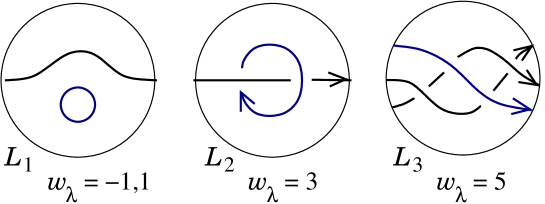
Figure 5. Elliptic quintic two-component links.

Proof.

The rank $r$ of the linear system defined by the plane section of $K\subset\mathbb{P}^{3}$ is at least $d-g=4$ by the Riemann-Roch theorem. By Lemma 11 we may assume that $K$ is obtained by deformation of a curve $\mathbb{R}K^{\prime}$ with a self crossing point $p$. By Proposition 12 the curve $C=\tilde{\pi}_{p}(K^{\prime})\subset{\mathbb{R}}{\mathbb{P}}^{2}$ in the corresponding nodal diagram is cubic of genus 1. Thus $C$ is smooth.

Suppose that $D^{-}\cap\mathbb{R}C=\emptyset$. Note that this determines the equivalence class of $D$ up to real deformations. In this case $\mathbb{R}K^{\prime}$ is topologically isotopic to the union of the planar cubic curve isotopic to $\mathbb{R}C$ and a solitary node at $p$. After a deformation the solitary node $p$ disappears. By Proposition 21 we have $w(K)=c=\pm 1$.

In other cases we have $D^{-}\subset\mathbb{R}C$. Then $\mathbb{R}K^{\prime}$ is obtained from $\mathbb{R}C\subset{\mathbb{R}}{\mathbb{P}}^{2}\subset{\mathbb{R}}{\mathbb{P}}^{3}$ by attaching the two lines connecting $p$ with the points of $D^{-}$ and then perturbing the result with the help of $D^{+}$. Note that up to equivalence $D^{+}$ is determined by the parity of the number of points in each connected component of $\mathbb{R}C\smallsetminus D^{-}$.

Suppose that $D^{-}$ is contained in the homologically non-trivial component $J$ of $\mathbb{R}C\subset{\mathbb{R}}{\mathbb{P}}^{2}$. Since $D$ is linearly equivalent to the hyperplane section of $\mathbb{R}C$ we must have even number of points in $\mathbb{R}C\smallsetminus J$ and different parities in the two arcs of $J\smallsetminus D^{-}$. Thus all such choices of $D$ are equivalent. Once again, $\mathbb{R}K\subset{\mathbb{R}}{\mathbb{P}}^{3}$ is topologically isotopic to a curve sitting in a plane and isotopic to $\mathbb{R}C$. We have $w(K)=c=\pm 1$.

If $\mathbb{R}K$ is of type II (i.e. $\mathbb{R}C$ is connected) then $J=\mathbb{R}C$ and there are no other possibilities for $D$. If $\mathbb{R}C$ is of type I (i.e. $\mathbb{R}K$ is a two-component link) then $w_{\lambda}(K)$ in both cases considered above coincides with $w(K)$.

If $\mathbb{R}K$ is a two-component link we also have additional cases. If $D^{-}$ has points in different components of $\mathbb{R}K$ this again determines the class of equivalence of $D$. Then $\mathbb{R}K$ is topologically isotopic either to $L_{1}$ or $L_{2}$ depending on the resolution at $p$. We have $w_{\lambda}(K)=\pm 2+c_{\lambda}$ in these cases by Proposition 21.

If $D^{-}\subset\mathbb{R}C\smallsetminus J$ then there are two equivalence classes of $D$. In one case we have odd number of points of $D^{+}$ in all three components of $\mathbb{R}C\smallsetminus D^{-}$. Then $w_{\lambda}(K)=\pm 4+c_{\lambda}$ and the topological type is $L_{2}$ or $L_{3}$ accordingly. In the other case both arcs of $\mathbb{R}C\smallsetminus(J\cup D^{-})$ have even number of points from $D^{+}$. Then $w_{\lambda}(K)=c_{\lambda}$ and the topological type is $L_{1}$.

To deduce the rigid isotopy classification it remains to prove that in our construction above the curves with the same $w_{\lambda}$ that are obtained from different cases considered above.

If $w_{\lambda}=3$ then there are two options for the distribution of $D^{-}$ between the components of $\mathbb{R}C$. If $D^{-}\subset\mathbb{R}C\smallsetminus J$ and $c=-1$ then $p$ corresponds to self-crossing of the topologically trivial (even) component of $\mathbb{R}K$. If $D^{-}\cap J\neq\emptyset$, $D^{-}\cap(\mathbb{R}C\smallsetminus J)=\emptyset$ and $c=+1$ then $p$ corresponds to the intersection point between different components of $\mathbb{R}K$.

If $w_{\lambda}=1$ then there are three options for the distribution of $D^{-}$ between the components of $\mathbb{R}C$. They correspond to self-intersection of an even component of $\mathbb{R}K$, the self-intersection of an odd component of $\mathbb{R}K$ and the intersection point of distinct components of $\mathbb{R}K$.

We claim that in the case $|w_{\lambda}|\leq 3$ there exists a real deformation of $K$ to an immersed curve $K^{\prime}$ with a single crossing point corresponding to distinct components of $K$. To see this we consider the projection of $K$ from a generic point $p$ on the even component of $\mathbb{R}K$. The image $B\subset\mathbb{P}^{2}$ of the projection is a quartic curve with two odd connected components of the normalization $\mathbb{R}K$. Being odd, these components must intersect at a point $r\in{\mathbb{R}}{\mathbb{P}}^{2}$. Since the curve $B$ is elliptic, there is a second nodal point of $\mathbb{R}B$ which must be either a self-intersection point $s\in{\mathbb{R}}{\mathbb{P}}^{2}$ of a component $P\subset\mathbb{R}K$ or an elliptic double point $s\in{\mathbb{R}}{\mathbb{P}}^{2}$ (the intersection of two complex conjugate branches of $B$).

If $s$ is elliptic then it corresponds to a pair $P_{s}\subset\mathbb{C}K\smallsetminus\mathbb{R}K$ of complex conjugate points in $\mathbb{R}K$ while $r$ corresponds to a pair $P_{r}\subset\mathbb{R}K$ of points from different components of $\mathbb{R}B$. Choose a plane $\mathbb{R}H$ passing through $P_{s}$ and a point $p^{1}_{r}\subset\ P_{r}$ from the odd component of $\mathbb{R}K$. The divisor $H\cap K$ on $K$ is equivalent to $D^{+}$ and consists of $P_{s}$, $p^{1}_{r}$ as well as another pair $P_{m}$ of points on $K$. If $P_{m}$ is contained in the odd component of $\mathbb{R}K$ then we can deform $P_{m}$ into $\mathbb{C}K\smallsetminus\mathbb{R}K$ not changing the linear equivalence class. If $P_{m}\cap\mathbb{R}K=\emptyset$ then we can further deform $P_{m}$ to the even component of $\mathbb{R}K$ within the same linear equivalence class.

If $P_{m}$ is contained in the even component of $\mathbb{R}K$ then we can deform $P_{m}$ (moving the image $p_{B}\in\mathbb{R}B$ of the projection point $p\in{\mathbb{R}}{\mathbb{P}}^{3}$ if needed) so that $D^{+}-\{p_{B}\}$ stays in the same linear equivalence class while the result of deformation of $D^{+}$ contains $P_{r}$. In this case the spatial curve corresponding to $(C,D)$ by Proposition 13 has a double point at $r$.

If $s$ is not elliptic then it corresponds to a self-intersection of one of the components of $\mathbb{R}K$. We choose a plane $\mathbb{R}H\subset{\mathbb{R}}{\mathbb{P}}^{3}$ passing through a point $p_{r}\in\mathbb{R}K$ and so that it separates the pair $P_{s}$ in the sense of Definition 16. Here we choose $p_{r}$ to be on the component $A\subset\mathbb{R}K$ containing the pair $P_{s}$.

Recall that we assume that $|w_{\lambda}|\leq 3$. By Proposition 21 this implies that if $A\cap D^{+}$ consists of more than 4 points then two of them bound an open interval $I\subset A$ disjoint from $D^{+}$ and $p_{B}$. Thus a pair of points of $D^{+}$ can be pushed to $\mathbb{C}K\smallsetminus\mathbb{R}K$ and then to the other component $A^{\prime}\subset\mathbb{R}K$. Note that $\tilde{\pi}_{p}|_{A^{\prime}}$ is an embedding since $P_{s}\subset A$. Thus we ensure that $D^{+}\cap A^{\prime}$ consists at least of two points. As in the case when $s$ is elliptic we deform these points (along with $p_{B}$ if needed) to ensure a crossing point between two different components of the spatial curve.

Thus any embedded curve with $d=5$, $g=1$ and $|w_{\lambda}|\leq 3$ is obtained by perturbing a nodal spatial curve with a node corresponding to crossing of different components. Therefore $w_{\lambda}$ determines the rigid isotopy type of type I $d=5$, $g=1$ real algebraic links. ∎

7. Rational knots of degree 6

Theorem 4.

There are 14 topological isotopy types (homeomorphism classes of pairs $({\mathbb{R}}{\mathbb{P}}^{3},\mathbb{R}K)$) of rational real algebraic curves $\mathbb{R}K$ of degree 6 embedded in the projective space ${\mathbb{R}}{\mathbb{P}}^{3}$. Figure 6 lists the knots.

Theorem 5.

There are 38 rigid isotopy types of rational real algebraic curves of degree 6 embedded in the projective space ${\mathbb{R}}{\mathbb{P}}^{3}$. Namely, each curve depicted on Figure 6 enhanced with a choice of the listed value for $w$ gives rise to one rigid isotopy class of $\mathbb{R}K$ in the depicted knot type. Furthermore, simultaneous reflection of $\mathbb{R}K$ in ${\mathbb{R}}{\mathbb{P}}^{3}$ and changing the sign of $w$ gives a new rigid isotopy type with the exception when the knot type of $\mathbb{R}K$ is amphichiral (the first two knots of Figure 6).

Figure 6. Real algebraic knots of degree 6 and genus 0.

7.1. Quartic nodal diagrams and odd arcs

Lemma 11 and Proposition 13 reduce Theorems 4 and 5 to classification of the nodal diagrams $(C,D)$ with respect to equivalences corresponding to topological and rigid isotopies of the resulting spatial curves.

Since $d=6$ the curve $C$ is a nodal quartic. Thus it has at most three real nodes. By Lemma 17 we may assume that $D$ is 3D-explicit. Thus we may apply Proposition 19.

Given a nodal diagram of $\mathbb{R}K^{\prime}$ we may consider parity of the number of elements of $A\cap D_{+}$ (counted with multiplicities) for any connected component $A\subset\mathbb{R}C\smallsetminus(\Sigma\cup D_{-})$. We refer to such components $A$ as diagram arc. A diagram arc $A$ is called odd if the parity of $A\cap D_{+}$ is odd, and even otherwise. Clearly, the parity of a diagram arc depends only on the underlying virtual knot diagram, so that we may speak of odd arcs of virtual nodal diagrams.

Proposition 22.

Suppose that $(C;D^{-},\tau,\sigma)$ is a virtual nodal diagram such that all nodes of a rational quartic curve $\mathbb{R}C$ are hyperbolic. The diagram $(C;D^{-},\tau,\sigma)$ is realizable by a $3D$-explicit nodal diagram $(C,D)$ if and only if the number of its odd arcs is at most 6.

Furthermore, in this case the virtual diagram $(C;D^{-},\tau,\sigma)$ and the sign $c$ of deformation of $K^{\prime}$ determine the embedded real algebraic curve $K\subset\mathbb{P}^{3}$ up to rigid isotopy.

Proof.

If the number of odd diagram arcs is greater than 6 then so must be the degree of the effective divisor $D^{+}$. Conversely, if this number is at most 6 then we may construct $D^{+}$ by selecting a point at each odd arc. If needed we add pairs of conjugate points on $C$ to ensure $\deg D^{+}=6$. The space of these choices is connected as any pair of points of $D^{+}$ on the same arc may be deformed off $\mathbb{R}C$ into $\mathbb{C}C\smallsetminus\mathbb{R}C$. ∎

7.2. Moves of the diagrams

Some nodal diagrams $(C,D)$ with distinct $C$ and $D$ correspond to the same rigid isotopy class of knots. We formulate the following straightforward proposition for nodal diagrams of rational curves of arbitrary degree $d$.

Proposition 23.

Suppose that nodal diagrams $(C_{1},D_{1})$ and $(C_{2},D_{2})$ of degree $d$ on rational curves $C_{j}$, $j=1,2$, of degree $d-2$ are 3D-explicit and related by means of one of the moves listed below.

Then the embedded real algebraic curves $K_{1},K_{2}\subset\mathbb{P}^{3}$ obtained from the corresponding curves $K^{\prime}_{1}$ and $K^{\prime}_{2}$ by resolving their double points in coherent directions are rigidly isotopic.

$\bullet$ (Moving a pole) Suppose that $C_{1}=C_{2}$. Let $u\in\Sigma$ be a hyperbolic node of $\mathbb{R}C=\mathbb{R}C_{1}=\mathbb{R}C_{2}$ and $u^{+},u^{-}\in\mathbb{R}K$ be two points corresponding to $u$ under the normalization $\nu:K\to C$. Let $u^{\pm}_{1}$ be the result of moving $u^{\pm}$ a little along $\mathbb{R}K$ in one (arbitrarily chosen) direction, and $u^{\pm}_{2}$ be the result of moving $u^{\pm}$ in the opposite direction. Let $D_{+}$ be an arbitrary real effective divisor on $K$ of degree $d-1$ disjoint from $\nu^{-1}(\Sigma)$, and $D^{-}$ be an arbitrary real effective divisor on $K$ disjoint from $\nu^{-1}(\Sigma)$ and $D^{+}$. Define $D^{\pm}_{j}=D^{\pm}\cup\{u^{\pm}_{j}\}$, $j=1,2$. (See Figure 7 for the change of the corresponding virtual nodal diagram.)

Figure 7. Moving a pole.

$\bullet$ (Annihilation of two poles) Suppose that $C_{1}=C_{2}$, and $D^{+}$ is an arbitrary real effective divisor of degree $d$ disjoint from $\Sigma$. Let $x\in\mathbb{R}K\smallsetminus(\nu^{-1}(\Sigma)\cup D^{+})$ be a point. Define $D^{-}_{1}$ to consist of two distinct points in $\mathbb{R}K$ close to $x$ and $D^{-}_{2}$ to be a pair of conjugate points in $\mathbb{C}K\smallsetminus\mathbb{R}K$ close to $x$.

The remaining three moves are algebro-geometric counterparts of the Reidemeister moves from knot theory. Here $C_{1}\neq C_{2}$, instead they are obtained as different real perturbations (within the class of real algebraic curves of degree $d$) of a certain curve $C_{0}\subset\mathbb{P}^{2}$. We denote the normalization of $C_{0}$ with $\nu_{0}:K_{0}\to C_{0}$ and consider a certain divisor $D_{0}=D^{+}_{0}-D^{-}_{0}$ on $K$ obtained as the difference of disjoint effective divisors $D^{\pm}_{0}$, $\deg D^{+}_{0}=d$, $\deg D^{-}_{0}=2$, with $D^{\pm}_{0}$ disjoint from the normalization of the nodes of $C_{0}$. In the following moves the divisor $D_{j}$, $j=1,2$, on the normalization $K_{j}\to C_{j}$ is obtained as an arbitrary small deformation of the divisor $D_{0}$ on $K_{0}$.

$\bullet$ (Reidemeister 1) Here $C_{0}$ is a curve with a single cusp $u$ and simple nodes as all other singularities, while $D_{0}$ is such that $D^{+}_{0}\ni u$. See Figure 2 for the corresponding virtual nodal diagrams.

$\bullet$ (Reidemeister 2) Here $C_{0}$ has a single tacnode $u$ and simple nodes as all other singularities, while the divisors $D^{\pm}_{0}$ are disjoint from $u$.

$\bullet$ (Reidemeister 3) Here $C_{0}$ is a curve with a single ordinary triple point $u$ and simple nodes as all other singularities, while $D^{+}_{0}$ contains a single point in the set $\nu_{0}^{-1}(u)$ (of cardinality 3).

Corollary 24.

Any embedded real rational curve of degree 6 is rigidly isotopic to a curve obtained from the curves whose virtual nodal diagrams are listed on Figure 8 by resolving them according to $c=\pm 1$ as in Lemma 11.

Each diagram $N^{c}_{\epsilon}$, where $N$ is the number of the diagram from Figure 8, $c=\pm$ is the sign of deformation of $K^{\prime}$ into $K$, and $\epsilon$ is the sum of the signs at all solitary nodes of $\mathbb{R}C$ (located in the region specified by the diagram) uniquely determines the rigid isotopy class of a real algebraic curve. Here the allowed values for $\epsilon$ are $\epsilon=\pm 1$ in the cases 20-22, 28 and 30; $\epsilon=0,-2$ in the case 26; $\epsilon=\pm 1,-3$ in the case 27; and $\epsilon=\pm 1,\pm 3$ in the case 29.

We omit $\epsilon$ from $N^{c}_{\epsilon}$ in the case when the diagram $N$ admits only one value for $\epsilon$ (e.g. if there are no solitary nodes at all).

Proof.

Once we ignore the sign of solitary nodes (i.e. the $\sigma$-data in virtual diagrams $(\mathbb{R}C;\mathbb{R}D^{-},\tau,\sigma)$, Figure 8 lists all triples $(\mathbb{R}C;\mathbb{R}D^{-},\tau)$ on a generically immersed quartics $C$ with not more than 6 odd arcs up to the equivalence generated by all moves from Proposition 23. We refer e.g. to [2] for classification of generic real quartics $C$.

Suppose that $C$ does not have elliptic nodes. In this case any 3D-explicit divisor defines a nodal diagram unless $C$ has a pair of conjugate nodes and $D$ is chosen so that the corresponding lift $K^{\prime}$ also have a pair of conjugate nodes. This means that the real meromorphic function corresponding to $D-H_{0}$, where $H_{0}$ is the divisor cut on $C\subset\mathbb{P}^{2}$ by the infinite axis of $\mathbb{P}^{2}$ has real values at a fixed pair of distinct and non-conjugate points of $\mathbb{C}C\smallsetminus\mathbb{R}C$. It is easy to see that the divisors with this property form a codimension 2 subspace in the connected real 8-dimensional space of all 3D-explicit divisors corresponding to the same virtual diagram.

Our next claim is that if $(C,D)$ is a 3D-explicit nodal diagram such that $C$ has a pair of conjugate nodes and a hyperbolic node then there exists a path $(C_{t},D_{t})$, $t\in[0,1]$, $(C_{0},D_{0})=(C,D)$ such that $(C_{t},D_{t})$ are 3D-explicit nodal diagrams,$C_{1}$ has three hyperbolic nodes, $C_{\frac{1}{2}}$ has a tacnode with two hyperbolic branches while the curve in $\mathbb{P}^{3}$ corresponding to $(C_{\frac{1}{2}},D_{\frac{1}{2}})$ by Proposition 13 is smooth outside of the projection point $p$. The family $(C_{t},D_{t})$ determines a rigid isotopy between the corresponding algebraic knots.

To prove the claim we note that there are two types of $(C,D)$ with such properties, and each can be obtained by perturbation of two ellipses in $\mathbb{P}^{2}$ intersecting transversally at two real points. It is sufficient to prove the claim for one representative curve in each type. The perturbations smooth one of the real transversal intersection points in two possible ways and keep the remaining one real and two imaginary points of the intersection of the ellipses. Both perturbations can be included in a one-parametric family of pairs of ellipses so that when $t$ increases the ellipses become tangent and then intersect transversely in 4 distinct real points producing a family $C_{t}$ of rational nodal quadrics. We define $D_{t}$ so that $(C_{t},D_{t})$ is 3D-explicit, and thus the corresponding curve $K^{\prime}_{t}\smallsetminus\{p\}\subset\mathbb{P}^{3}$ is smooth.

Lemma 25 allows us to reduce consideration of nodal diagrams with elliptic nodes to those without elliptic nodes and thus finishes the proof. In particular, cases 26 with $\epsilon=+2$ as well as 27 with $\epsilon=+3$ can not appear as the corresponding diagrams with hyperbolic nodes have more than 6 odd arcs. ∎

Lemma 25.

Any real smooth rational sextic $K\subset\mathbb{P}^{3}$ is rigidly isotopic to a curve obtained from a nodal diagram such that the underlying real quartic rational curve does not have elliptic nodes.

Proof.

Let $q\in\mathbb{R}C$ be an elliptic node in the nodal diagram $(C,D)$ of $K$. The image of $C$ under the quadratic transformation centered in the nodes of $C$ is a conic intersecting the coordinate line corresponding to $q$ in two imaginary points. A deformation of this conic to a conic intersecting this line in two real points give a deformation $C_{t}$, $t\in[0,1]$, of $C=C_{0}$ into a rational nodal quartic $C_{1}$ that changes $q$ into a hyperbolic node, and leaves the other nodes of $C$ unchanged. This deformation can be extended to a deformation $D_{t}$ of $D=D_{0}$ so that $D_{t}$ remains disjoint from the nodes of $C_{t}$ and neither $D^{+}_{t}$ nor $D^{-}_{t}$ has multiple points.

This gives a deformation $K^{\prime}_{t}\subset\mathbb{P}^{3}$ of sextic curves. If $K^{\prime}_{t}\smallsetminus\{p\}$ is nonsingular then the smooth curves obtained by coherent deformations of $K^{\prime}_{0}$ and $K^{\prime}_{1}$ are rigidly isotopic while the number of elliptic points of $C_{1}$ is less than that of $C_{0}$, so that we may proceed inductively. Suppose that $K^{\prime}_{t}\smallsetminus\{p\}$ is singular for $t=\epsilon$ and nonsingular for $t\in[0,\epsilon)$.

Note that the singularity of $K^{\prime}_{t}\smallsetminus\{p\}$ must sit over an elliptic node $s$ of $C_{t}$ since $D$ is 3D-explicit. Exchanging the roles of $s$ and $p$ if needed, we may assume that $p$ was elliptic, i.e. $D^{-}\cap\mathbb{R}K=\emptyset$. In such case $\mathbb{R}K\smallsetminus\nu^{-1}(\Sigma)$ consists of not more that 6 arcs, and $D^{+}$ maybe deformed in a family $D_{t}$ of divisors in the same curve $K$ so that $D^{-}_{t}=D^{-}$, $D^{+}_{t}\cap D^{-}_{t}=\emptyset$, $D^{+}_{t}\cap\nu^{-1}_{1}(\Sigma)=\emptyset$, $t=[0,1)$, while $D^{+}_{1}=\nu^{-1}(\Sigma)$, so that $K^{\prime}_{1}\subset\mathbb{P}^{3}$ is a quadrinodal sextic curve, i.e. a curve with 4 distinct nodes. Note that by our construction these 4 nodes are not coplanar and the curve $K^{\prime}_{t}$ is not contained in any plane of $\mathbb{P}^{2}$. If there are nodes forming a complex conjugate pair then we can proceed as in the proof of Corollary 24 deforming this pair to a pair of hyperbolic nodes.

If all nodes are real (elliptic or hyperbolic) then we choose the coordinates in $\mathbb{P}^{3}$ so that the intersections of the coordinate hyperplanes correspond to the nodes of $K^{\prime}_{1}$, the cubic transformation

(2) $$(x_{0}:x_{1}:x_{2}:x_{3})\mapsto(\frac{1}{x_{0}}:\frac{1}{x_{1}}:\frac{1}{x_{2}}:\frac{1}{x_{3}})$$

maps $K^{\prime}_{t}$ to a conic in $\mathbb{P}^{3}$. Thus all quadrinodal curves corresponding to the same planar nodal quartic $C$ are isotopic. But all elliptic nodes of $C$ can be simultaneously deformed to hyperbolic nodes as we can see through consideration of conics in $\mathbb{P}^{2}$ tangent to coordinate lines.

It remains to prove that we can deform $(C,D)=(C_{0},D_{0})$ to $(C_{1},D_{1})$ so that all $(C_{t},D_{t})$, $t\in[0,1)$ are nodal diagrams while $K^{\prime}_{1}\subset\mathbb{P}^{3}$ is quadrinodal. We start with a deformation of $D$ on the same curve $K$ as considered above. If there exists $\epsilon<1$ with singular $K^{\prime}_{\epsilon}\smallsetminus\{p\}$ then its singularity must be an elliptic node $e$. Consider a plane section $H$ of $K^{\prime}_{\epsilon}$ disjoint from $\{p\}$ and such it passes through $e$ and such that the corresponding divisor is 3D-explicit (we can do that since there are not more than 2 hyperbolic nodes of $C$). Deforming the plane section from $D^{+}_{\epsilon}$ to $H$ gives us a family of intermediate nodal diagrams $(C_{t},D_{t})$, $t\in[\epsilon,\epsilon_{H})$, $\epsilon<\epsilon_{H}<1$ while $D_{\epsilon_{H}}^{+}$ contains $\nu_{\epsilon_{H}}^{-1}(e)$. We continue the process by deformation of the effective divisor $D_{\epsilon_{H}}^{+}-\nu_{\epsilon_{H}}^{-1}(\Sigma_{\epsilon_{H}}\smallsetminus\{e\})$ until we arrive to $D_{1}=\nu^{-1}_{1}(\Sigma_{1})$. Finally we perturb the family $(C_{t},D_{t})$ slightly to ensure that it consists if nodal diagrams for $t<1$.

∎

Figure 8. Equivalence classes of the diagrams of $\mathbb{R}K^{\prime}$ with respect to the moves of Proposition 23.

7.3. Quadrinodal spatial rational sextics and isotopy

The quadrinodal curves we considered in the previous subsection are also useful for finding isotopies among the curves listed in Corollary 24. Let $J\subset\mathbb{P}^{3}$ be a quadrinodal rational sextic with the nodes in $(1:0:0:0)$, $(0:1:0:0)$, $(0:0:1:0)$ and $p=(0:0:0:1)$.

Proposition 26.

For every choice of signs for some nodes of a real rational quadrinodal sextic curve $J$ there exists a deformation of $\mathbb{R}J$ in the class or real rational sextics resolving those nodes according to the chosen signs and keeping all the other nodes unperturbed.

Proof.

The curve $J$ corresponds to a nodal rational planar curve $C$ and the divisor $D^{+}$ consisting of 6 points in the normalization $K$ of $C$ corresponding to 3 nodes of $C$ so that each node corresponds to a pair of points in $D^{+}$. Moving one of the points in the pair in an appropriate direction we get the deformation of $\mathbb{R}J$ with the chosen sign. (In the case when the pair consists of complex conjugate points we move the second point in a complex conjugate way.) If our choice of signs keeps some of the nodes unresolved then without loss of generality we may assume that we do not resolve $p$. If our choice resolve all the nodes then we apply Lemma 11 to resolve $p$. ∎

The normalization of $\mathbb{R}J$ is topologically a circle. Hyperbolic nodes of $J$ may be encoded on this circle by means of the so-called chord diagram: we draw a chord connecting each pair of points that gets identified to a node of $\mathbb{R}J$. Real solitary nodes of $J$ are ignored in the chord diagram $S$, their number is equal to 4 minus the number of chords. As the space of $n$ distinct pairs of complex conjugate points in $\mathbb{C}\mathbb{P}^{1}$ is connected we obtain the following statement.

Proposition 27.

The space of real quadrinodal rational sextic curves in $\mathbb{P}^{3}$ (considered up to projective linear transformations) corresponding to the same combinatorial diagram of real chords is connected.

Here we consider only quadrinodal curves with all nodes real, i.e. without complex conjugate pairs of nodes.

7.4. Completing the classification

Proof of Theorems 4 and 5.

By Corollary 24 to deduce the classification we need to identify the curves obtained from the diagrams of Figure 8 that are rigidly isotopic. For this we use eleven real rational quadrinodal curves given by the chord diagrams A through K depicted on Figure 10 as well as the 3-nodal curve L from Figure 9.

Figure 9. A trinodal rational sextic curve.

Figure 10. Eleven quadrinodal sextic curves.

The quadrinodal curves are depicted along with 4 projections from each of its nodes (numbered 1 through 4). For convenience we indicate the diagram of the one-nodal curve $\mathbb{R}K^{\prime}$ obtained by positive resolution of all nodes except for the projection point. To identify different projections of the same quadrinodal curve we indicate the same arc connecting two of the nodes.

Also we depict the lower and upper half arcs near the points of $D_{-}$ for the corresponding diagrams. Note that this choice is determined (up to simultaneous reversal) by the following rule. Let us connect the two points of $D_{-}$ by an arc in the curve $\mathbb{R}C\subset{\mathbb{R}}{\mathbb{P}}^{2}$ and compute the number of points of $D_{+}$ contained on this arc. If the arc crosses the infinite line of the projective plane of the diagram odd number of times then we add one to this number. If the result is odd then the arc connects a lower half-arc to an upper half arc. Otherwise it connects the half-arcs of the same kind.

The tri-nodal curve in Figure 10 (curve “L”) is parameterized by

$$t\mapsto(p_{1}p_{3}p_{5}p_{6}p_{7}p_{8}:p_{1}p_{2}p_{3}p_{4}p_{5}p_{7}:p_{2}p_{4}p_{6}^{3}p_{8}:p_{1}p_{2}p_{4}p_{5}p_{6}p_{8}),$$

where $p_{i}=t-t_{i}$ and $t_{1}<t_{2}<\dots<t_{8}$.

Figure 11. Graphs of rigid isotopy equivalence.

Figure 11 indicates which of the curves obtained from the diagrams of Figure 10 are rigidly isotopic. Namely, Figure 11 lists bipartite graphs with two type of vertices: numeric and alphabetic. The number of the numeric vertices refers to the diagram number from Figure 8 as well as the sign used for the perturbation of the node. Each such diagram encodes the equivalence class with respect to the moves of Proposition 23.

The letter of the alphabetic vertices refers to the multinodal curves from Figure 10. Each edge is labeled by the number of the node of the corresponding multinodal curve that becomes the projection point in the diagram for the adjacent numeric vertex. The signs of the resolution used in the graph are determined by the signs at the adjacent numerical vertices.

We see that each pair consisting of a curve from Figure 6 and the non-negative value of its Viro invariant $w$ corresponds to a connected subgraph and that each resolution of a curve from Figure 8 is contained in one of the subgraphs. Different knots from Figure 6 are topologically different as knots in ${\mathbb{R}}{\mathbb{P}}^{3}$, see [3]. Figure 12 provides topological identification of the boxed resolved diagram in Figure 11 and the corresponding knot type from Figure 6.

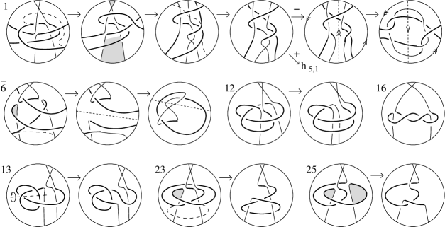
Figure 12. Identifications between the knots from Figure 6 and the boxed diagrams of Figure 11.

A reflection (an orientation-reversing automorphism) in ${\mathbb{R}}{\mathbb{P}}^{3}$ reverses the knot together with its Viro invariant. Thus each curve with positive $w$ corresponds to two distinct rigid isotopy types under reflection while a curves with $w=0$ may correspond to one or two types. We have four types of knots with $w=0$: $K_{1}$, $K_{2}$, $K_{5}$ and $K_{6}$. The knots $K_{5}$ and $K_{6}$ are chiral: they are not topologically isotopic to their reflection in ${\mathbb{R}}{\mathbb{P}}^{3}$ as the two components of their inverse images under the universal covering ${\mathbb{S}}^{3}\to{\mathbb{R}}{\mathbb{P}}^{3}$ have non-zero linking number. In the same type the knot types $K_{1}$ and $K_{2}$ are amphichiral. Furthermore, the corresponding real algebraic sextics are rigidly isotopic as their reflections appear in the same components of the graphs from Figure 11. Altogether we get 38 rigid isotopy types in Theorem 5. We get 14 topological types of Theorem 4 by taking out the Viro invariant information from the data. ∎

8. Elliptic knots and links of degree 6

Theorem 6.

There are 16 topological isotopy types (homeomorphism classes of pairs $({\mathbb{R}}{\mathbb{P}}^{3},\mathbb{R}L)$) of elliptic (genus 1) smooth real algebraic curves $K$ of degree 6 in the projective space ${\mathbb{R}}{\mathbb{P}}^{3}$ in the case when $\mathbb{R}K$ is a two-component link. Namely, Figure 13 lists the links.

There are 4 such types in the case when $\mathbb{R}L$ is connected. Namely, the types $K_{1},K_{3},K_{5},K_{6}$ from Figure 6 are realizable by smooth elliptic sextic curves in $\mathbb{P}^{3}$.

Theorem 7.

There are 40 rigid isotopy types of rational real algebraic curves of degree 6 embedded in the projective space ${\mathbb{R}}{\mathbb{P}}^{3}$ in the case when $\mathbb{R}K$ is a two-component link. Namely, each curve depicted on Figure 13 enhanced with a choice of the listed value for $w_{\lambda}$ gives rise to one rigid isotopy class of $\mathbb{R}K$ in the depicted link type. Furthermore, simultaneous reflection of $\mathbb{R}K$ in ${\mathbb{R}}{\mathbb{P}}^{3}$ and changing the sign of $w_{\lambda}$ gives a new rigid isotopy type with the exception of when $\mathbb{R}K$ is a topologically trivial link (the first case in Figure 13).

There are 12 such types in the case when $\mathbb{R}K$ is connected. Namely, we may have $w_{\lambda}=\pm 3,\pm 1$ for the types $K_{1}$; $w_{\lambda}=3$ for $K_{3}$; $w_{\lambda}=1,3$ for $K_{5}$; and $w_{\lambda}=1$ for $K_{6}$ (see Figure 6).

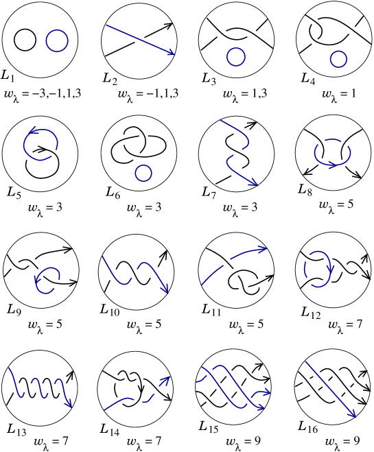
Figure 13. Two-component real algebraic links of degree 6 and genus 1.

8.1. Binodal planar elliptic quartics

To prove Theorems 6 and 7 we use a technique similar to that developed in the previous section with some modifications. Lemma 11 and Propositions 12 and 13 reduce the proof to studying of nodal diagrams $(C,D)$, where $C$ is a nodal elliptic curve of degree 4 while $D=D^{+}-D^{-}$ is linearly equivalent to a hyperplane section of $C$. Namely, the nodal diagram $(C,D)$ defines a spatial curve $K^{\prime}\subset\mathbb{P}^{3}$ with the node $p=(0:0:0:1)\in\mathbb{P}^{3}$ that can be resolved in two ways to a smooth spatial elliptic sextic. Once again, we can distinguish between positive and negative resolution of $p$. If $p$ is the self-intersection of the same component of $\mathbb{R}K$ then we may use any of its orientations to determine the sign. If $p$ is the intersection of different components then $K$ is necessarily of type I and we may use a complex orientation of $\mathbb{R}K$ to determine the sign.

The singular set $\Sigma\subset C$ consists of two nodes. Thus the four points of $\nu^{-1}(\Sigma)\subset K$ give a hyperplane section of $C$ through the normalization map $\nu:K\to C$.

Let $E$ be an abstract elliptic curve (not embedded to any projective space) enhanced with an antiholomorphic involution $\operatorname{conj}$ with non-empty fixed locus $\mathbb{R}E$. Let $\operatorname{ch}_{j}\subset E$, $j=1,2$, be two disjoint pairs of points with $\operatorname{conj}(\operatorname{ch}_{j})=\operatorname{ch}_{j}$.

Lemma 28.

If the divisors formed by $\operatorname{ch}_{1}$ and $\operatorname{ch}_{2}$ are not linearly equivalent in $E$ then there exists a planar nodal quartic curve $C\subset\mathbb{P}^{2}$ with two nodes $q_{j}\in C$, $j=1,2$, with $(K;\nu^{-1}(q_{1}),\nu^{-1}(q_{2}))$ is isomorphic to $(E;\operatorname{ch}_{1},\operatorname{ch}_{2})$.

Vice versa, for any nodal irreducible quartic curve $C$ with two nodes $q_{j}\in C$, $j=1,2$, the divisors $\nu^{-1}(q_{1})$ and $\nu^{-1}(q_{2})$ are not linearly equivalent.

Proof.

Consider the projective linear system $|\operatorname{ch}_{1}+\operatorname{ch}_{2}|$ and a point $r\in E\smallsetminus(\operatorname{ch}_{1}\cup\operatorname{ch}_{2})$. As $\dim|\operatorname{ch}_{1}+\operatorname{ch}_{2}|=3$ there exist a unique point $r_{j}$, $j=1,2$, such that $r_{j}+r+\operatorname{ch}_{j}$ is equivalent to $\operatorname{ch}_{1}+\operatorname{ch}_{2}$. Since $|\operatorname{ch}_{1}|\neq|\operatorname{ch}_{2}|$ we have $r_{1}\neq r_{2}$, and $\operatorname{ch}_{1}+\operatorname{ch}_{2},r_{1}+r+\operatorname{ch}_{1},r_{2}+r+\operatorname{ch}_{2}$ generate a 2-dimensional subsystem in $|\operatorname{ch}_{1}+\operatorname{ch}_{2}|$ and a map of $E$ to $\mathbb{P}^{2}$. Note that the image of $E$ has two nodes corresponding to $\operatorname{ch}_{j}$. Thus this subsystem contains $s_{j}+s+\operatorname{ch}_{j}$ for with some $s_{j}$ for every $s\in E\smallsetminus(\operatorname{ch}_{1}\cup\operatorname{ch}_{2})$. Therefore, the resulting linear system is independent of the choice of $r$.

For the converse it suffices to take a generic point in a nodal elliptic quartic curve $C\subset\mathbb{P}^{2}$ and connect it with the nodes $q_{j}$ of $C$ by lines. The lines will intersect $C$ at distinct fourth points. Distinct single points are not linear equivalent since our normalization $K$ is not rational. ∎

This allows us to work with planar nodal elliptic quartics almost as freely as with planar nodal rational quartics.

Corollary 29.

There are 10 distinct rigid isotopy classes of real elliptic quartic curves in $\mathbb{P}^{2}$ in the case when the normalization of the real locus consists of two components: 5 with both nodes hyperbolic, 2 with one hyperbolic and one elliptic node, 1 with two elliptic nodes and 2 with a pair of complex conjugate nodes. There are 5 distinct classes in the case when the normalization is connected: 2 with both nodes hyperbolic, 1 with with one hyperbolic and one elliptic node, 1 with two elliptic nodes and 1 with a pair of complex conjugate nodes.

Here by rigid isotopy we mean a deformation in the class of (irreducible) real elliptic binodal quartics in $\mathbb{P}^{2}$.

Proof.

It is convenient to think of $\operatorname{ch}_{j}$ as a chord connecting two points of the real locus $\mathbb{R}E$. We have three deformation classes if each chord connects two points from the same component of $\mathbb{R}E$, and a single class if one or both chords connect different components of $\mathbb{R}E$. Each class is unique to automorphism and deformation of $(E;\operatorname{ch}_{1},\operatorname{ch}_{2})$ in the class of triples with $|\operatorname{ch}_{1}|\neq|\operatorname{ch}_{2}|$. If $\mathbb{R}E$ is disconnected then complex conjugate nodes may correspond to intersections of the same or different components, this gives us two classes. ∎

8.2. Nodal diagrams in the elliptic case

Propositions 22 has the following counterpart for the case of genus 1.

Proposition 30.

Suppose that $(\mathbb{R}C;\mathbb{R}D^{-},\tau,\sigma)$ is a virtual nodal diagram such that all nodes of a nodal elliptic quartic curve $\mathbb{R}C$ are hyperbolic. The diagram $(\mathbb{R}C;\mathbb{R}D^{-},\tau,\sigma)$ is not realizable by a 3D-explicit nodal diagram $(C,D)$ if the six-point set $D^{-}\cup\nu^{-1}(\Sigma)$ is contained in a connected component of $\mathbb{R}K$. It is also not realizable if $D^{-}\cup\nu^{-1}(\Sigma)\subset\mathbb{R}K$ and $\mathbb{R}C$ has a node corresponding to intersection of distinct components of $\mathbb{R}K$.

In all other cases $(\mathbb{R}C;\mathbb{R}D^{-},\tau,\sigma)$ is realizable by a 3D-explicit nodal diagram $(C,D)$. Furthermore, the virtual diagram $(\mathbb{R}C;\mathbb{R}D^{-},\tau,\sigma)$ together with the sign $c$ of deformation of $K^{\prime}$ determine the embedded real algebraic curve $K\subset\mathbb{P}^{3}$ up to rigid isotopy.

Proof.

Suppose $(C,D)$ is a 3D-explicit nodal diagram. The number of arc-components of $\mathbb{R}K\smallsetminus(\nu^{-1}(\Sigma)\cup D^{-})$ is 6 if $D^{-}\subset\mathbb{R}K$, otherwise it is 4. Suppose that we have 6 odd arcs. Then all 6 points of $D^{+}$ are real, and each point sits on its own arc of $\mathbb{R}K\smallsetminus(\nu^{-1}(\Sigma)\cup D^{-})$. If all these 6 points belong to the same component of $\mathbb{R}K$ we have a contradiction to the Abel theorem as $|D^{+}|=|D^{-}+\nu^{-1}(\Sigma)|$, but a divisor cannot be principal if it can be presented as the boundary of a collection of disjoint coherently oriented intervals contained in the same component of $\mathbb{R}K$.

If the images of different components of $\mathbb{R}K$ under $\nu$ intersect then by Corollary 29 there are just two possibilities for $\mathbb{R}C$ up to rigid isotopy. In this case $K$ is of type I. Note that if $f:K\to\mathbb{P}^{1}$ is a real meromorphic function with $f^{-1}({\mathbb{R}}{\mathbb{P}}^{1})=\mathbb{R}K$ then $f$ has no real critical values, and a complex orientation of $\mathbb{R}K$ can be obtained as the pullback of an orientation of ${\mathbb{R}}{\mathbb{P}}^{1}$. Applying this remark to the function defined by $D^{+}-(D^{-}+\nu^{-1}(\Sigma))$ for these two possibilities we get a contradiction, see Figure 14. In the remaining cases existence and uniqueness of a nodal diagram $(C,D)$ up to deformation follows from Lemma 28, where the black points represent $f^{-1}(\infty)$ (i.e. the divisor $D^{-}+\nu^{-1}(\Sigma)$) and the white points represent $f^{-1}(\epsilon)$ with $\epsilon\gg 0$. ∎

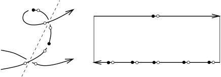
Figure 14. Six odd arcs and the Abel theorem.

Lemma 31.

Any real smooth rational sextic $K\subset\mathbb{P}^{3}$ is rigidly isotopic to a curve obtained from a nodal diagram such that the underlying real quartic rational curve does not have elliptic nodes.

Proof.

Suppose that $(C,D)$ is a 3D-explicit nodal diagram, and $C$ has an elliptic node. Use Lemma 28 to deform the corresponding chord to a tangent line, and then further to real chord. Then the elliptic node gets deformed to a cusp, and further to a hyperbolic node. Deform $D$ in its linear equivalence class to extend the deformation of $C$ to a 3D-explicit deformation $(C_{t},D_{t})$ of $(C,D)$. We can do that since we may assume that $\deg(D^{+}\cap\mathbb{R}K)\leq 4$ since $\mathbb{R}K\smallsetminus(\nu^{-1}(\Sigma)\cup D^{-})$ contains at most of four arcs.

If during the deformation the curve $K^{\prime}_{t}\smallsetminus\{p\}\subset\mathbb{P}^{3}$ has a singular point then it must be an elliptic node. Thus exchanging the roles of $p$ and this node we may assume that $p$ is elliptic, i.e. $D^{-}\cap\mathbb{R}K=\emptyset$. In this case we may assume that $\deg(D^{+}\cap\mathbb{R}K)\leq 2$ and keep two of the points of $D^{+}_{t}$ at the inverse image of the elliptic node of $C_{t}$ under $\nu$. If $C_{t}$ has two elliptic nodes then $D^{+}_{t}$ can be chosen without real points and we may keep four points of $D_{t}^{+}$ at $\nu^{-1}(\Sigma)$ thus ensuring (after a perturbation) that $K^{\prime}_{t}\smallsetminus\{p\}$ is smooth. ∎

Corollary 32.

Any real elliptic curve $K$ of degree 6 in $\mathbb{P}^{3}$ is rigidly isotopic to a curve obtained from one of the curves whose virtual nodal diagrams are listed on Figure 15 by resolving them according to $c=\pm 1$ as in Lemma 11 if $K$ is of type I.

Each diagram $N^{c}_{\epsilon}$, where $N$ is the number of the diagram from Figure 15, $c=\pm$ is the sign of deformation of $K^{\prime}$ into $K$, and $\epsilon$ is the sum of the signs at all solitary nodes of $\mathbb{R}C$ (located in the region specified by the diagram) uniquely determines the rigid isotopy class of a real algebraic curve. Here the allowed values for $\epsilon$ are $\epsilon=\pm 1$ in the cases 17 and 18; $\epsilon=0,-2$ in the cases 22 and 23; and $\epsilon=0,\pm 2$ in the cases 24 and 25.

If $K$ is of type II then it is rigidly isotopic to a curve obtained from is rigidly isotopic to a curve obtained from one of the curves whose virtual nodal diagrams are listed on Figure 8, cases 20, 21, 22 (without further elliptic nodes), 26 with $\epsilon=-1$, 27 with $\epsilon=0,-2$, or 29 with $\epsilon=\pm 2,0$, by resolving them according to $c=\pm 1$.

Figure 15. Equivalence classes of the diagrams of $\mathbb{R}K^{\prime}$ with respect to the moves of Proposition 23.

Proof.

The proof is similar to that of Corollary 24. Note that if the number of odd arcs is not more than 4 then we have the moves of Proposition 23 also for the genus 1 case. ∎

8.3. Trinodal spatial elliptic sextics and proof of Theorems 6 and 7

Additional isotopies among the curves corresponding to positive and negative resolution of nodal diagrams from Figure 15 are obtained with the help of bi- and trinodal spatial elliptic sextics. As in the case of quadrinodal rational sextics we may resolve the nodes of such curves independently according to our choice of signs.

Lemma 33.

Let $J\subset\mathbb{P}^{3}$ be a rational real quadrinodal sextic and $p\in J$ be one of its real nodes (can be elliptic or hyperbolic). We may choose to smooth $J$ at $p$ to a real elliptic sextic $I$ of a type I or to a type II keeping three other nodes of $J$.

Proof.

We have seen that $J$ is given by 4 chords on a conic $Q\subset\mathbb{P}^{2}$. We can view the chords as lines in $\mathbb{P}^{2}$. Perturbing the diagram if needed we may assume that no three chords intersect in a point. The plane $p^{2}$ can be linearly embedded to $\mathbb{P}^{3}$ so that the four chords are cut by the coordinate planes. Then $J$ is the image of $Q$ under (2).

Let the line $L_{p}\subset\mathbb{P}^{2}$ be the chord corresponding to $p$. Let $R\subset\mathbb{P}^{2}$ be the cubic curve obtained by perturbation of $J\cup L_{p}$ with the help of the three other chords (either to a type I or type II real curve). The image of $R$ under (2) is $I$. ∎

Proof of Theorems 6 and 7. Suppose that $K$ is of type II. We use the same quadrinodal curves as in Figure 10 and apply to them Lemma 33 to complete the classification in this case.

If $K$ is of type I we use trivalent curves from Figure 16 to relate the curves from Corollary 32 with graphs depicted at Figure 17. All the nodal curves in Figure 15 except for J can be obtained from rational nodal curves of Figures 9 and 10 with the help of Lemma 33 (see Table below). It is easy to construct J explicitly.

Rational multinodal curve	A	B	C	H	J	H	I	J	K	L	L
Perturbed node	1	2	2	2	3	1	4	1	1	3	1
Elliptic multinodal curve	A	B	C	D	E	F	G	H	I	K	L

Figure 16. Twelve trinodal and binodal elliptic curves

Figure 17. Graphs of rigid isotopy equivalence.

∎

References

- [1] Björklund, Johan, Real algebraic knots of low degree, J. Knot Theory Ramifications, 20:9 (2011), 1285–1309.
- [2] D’Mello, Shane, Rigid isotopy classification of real degree-4 planar rational curves with only real nodes (An elementary approach), arXiv:1307.7456.
- [3] Drobotukhina, J., Classification of links in with at most six crossings, Advances in Soviet Math., 18 (1994), 87–121.
- [4] Harnack, Axel, Über die Vieltheiligkeit der ebenen algebraischen Curven, Math. Ann., 10:2 (1876), 189–198.
- [5] Hilbert, David, Mathematical problems, Bull. Amer. Math. Soc. 8 (1902), 437–479.
- [6] Rokhlin, V. A., Complex topological characteristics of real algebraic curves, Uspehi Mat. Nauk, 33:5 (1978), 77-89.
- [7] Viro, Oleg, Encomplexing the writhe, Amer. Math. Soc. Transl. Ser. 2, 202 (2001), 241–256.