The Orbit and Mass of the Third Planet in the Kepler-56 System

Abstract

While the vast majority of multiple-planet systems have orbital angular momentum axes that align with the spin axis of their host star, Kepler-56 is an exception: its two transiting planets are coplanar yet misaligned by at least 40 degrees with respect to the rotation axis of their host star. Additional follow-up observations of Kepler-56 suggest the presence of a massive, non-transiting companion that may help explain this misalignment. We model the transit data along with Keck/HIRES and HARPS-N radial velocity data to update the masses of the two transiting planets and infer the physical properties of the third, non-transiting planet. We employ a Markov Chain Monte Carlo sampler to calculate the best-fitting orbital parameters and their uncertainties for each planet. We find the outer planet has a period of $1002\pm 5$ days and minimum mass of $5.61\pm 0.38$ M${}_{\textrm{Jup}}$. We also place a 95% upper limit of 0.80 m s^-1 yr^-1 on long-term trends caused by additional, more distant companions.

1. Introduction

Red giant Kepler-56 (KOI-1241, KIC 6448890) is an atypical star to host transiting planets. While the vast majority of known transiting planets orbit solar-type FGK stars (Batalha et al., 2013; Burke et al., 2014; Mullally et al., 2015; Rowe et al., 2015; Grunblatt et al., 2016; Van Eylen et al., 2016), Kepler-56 is one of only a few post-main sequence stars known to host them (Lillo-Box et al., 2014; Ciceri et al., 2015; Quinn et al., 2015; Pepper et al., 2016). Detecting transits of these stars is difficult because they are much larger than main sequence stars and have higher levels of correlated noise (Barclay et al., 2015). As such, when selecting targets for Kepler , mission scientists prioritized capturing main sequence FGK stars over other stellar types (Batalha et al., 2010).

Nevertheless, Kepler-56 was targeted in the original Kepler mission (Borucki et al., 2010), and two transiting planet candidates with periods of $10.50$ and $21.41$ days were identified in the first data release (Borucki et al., 2011). These candidates interacted dynamically, with observed, anticorrelated variations in their times of transit (Ford et al., 2011, 2012; Steffen et al., 2012). Steffen et al. (2013) analyzed the times of transit and the orbital stability of the system to confirm these two candidates as planets, making Kepler-56 the latest stage star known at the time to host multiple transiting planets.

As a red giant, Kepler-56 exhibits convection-driven oscillations that vary on timescales long enough to be observable with Kepler long-cadence photometry. Huber et al. (2013) analyzed its observed asteroseismic modes to infer a stellar mass of $1.32\pm 0.13$ M_⊙ and radius of $4.23\pm 0.15$ R_⊙. Through radial velocity (RV) and transit timing observations of the transiting planets, Huber et al. (2013) then determined their masses to be $22.1^{+3.9}_{-3.6}$ M_⊕ and $181^{+21}_{-19}$ M_⊕, respectively. Through a combination of asteroseismology and dynamical instability simulations, they also detected that the orbits of the planets, while coplanar with each other, are tilted with respect to the axis of stellar rotation by $\sim 45$ degrees.

Huber et al. (2013) also detected the presence of a long-term RV acceleration in the data consistent with at least one additional massive companion. While the acceleration by itself cannot provide a unique orbit for the outer companion, they proposed that both the planetary obliquity and long-term RV trend could be explained by a non-transiting companion with a period of $900$ days and mass $3.3$ M${}_{\textrm{Jup}}$.

However, the duration of their RV observations only covered a baseline of $\sim 100$ days. Equipped with four more years of RV data, we are now able to measure the orbital parameters of this purported planet, which has the third-longest orbital period of any confirmed planet orbiting a Kepler star (Kostov et al., 2015; Kipping et al., 2016). We are also able to place upper limits on the presence of additional planets from the lack of additional long-term trends in the RV curve.

In Section 2 we describe our data collection and reduction. In Section 3, we describe our RV model. In Section 4, we present our best estimates for this planet’s orbital parameters, as well as the likelihood of another companion. We discuss our results in Section 5 and summarize our findings in Section 6.

2. Data Collection and Analysis

Our analysis is based on 43 RV observations of Kepler-56 obtained from 2013 to 2016 with two different spectrographs: 24 with Keck/HIRES (Vogt et al., 1994) and 19 with HARPS-North (Cosentino et al., 2012).

2.1. Keck/HIRES Observations

Our Keck/HIRES observations were obtained largely following the standard procedures of the California Planet Survey (CPS) team (Howard et al., 2010), modified slightly for the faint stars of the Kepler field, following the approach of Huber et al. (2013). For all observations, we used the C2 decker (14$\farcs$0 $\times$ 0$\farcs$85), which is a factor of four taller than the B5 decker typically used for observations of bright stars. This setup allows for more background light to enter the spectrograph, allowing for better sky-subtraction while maintaining a resolving power of $R\approx$ 50,000.

Each observation was made with an iodine cell mounted along the light path before the entrance to the spectrograph. The iodine spectrum superposed on the stellar spectrum provides a precise, stable wavelength scale and information on the shape of the instrumental profile of each observation (Valenti et al., 1995; Butler et al., 1996).

The integration times range from 600 to 1800 seconds. The star-times-iodine spectrum was modeled using the Butler et al. (1996) method, with the instrumental profile removed through numerical deconvolution. The RV of the star at each observation is compared to a template spectrum of the star obtained without iodine, with the instrumental profile removed through numerical deconvolution. The observed RVs are listed in Table 1.

The data set used here includes the 10 observations used by Huber et al. (2013), reanalyzed after all observations were recorded. An improved stellar template spectrum causes the measured RV from these observations to be slightly different than those reported by Huber et al. (2013), although the differences are smaller than the formal uncertainties on each observation.

2.2. HARPS-North Observations

We also obtained 19 observations of Kepler-56 with HARPS-North, a high-precision echelle spectrograph at the 3.6 m Telescopio Nazionale Galileo (TNG) at the Roque de los Muchachos Observatory, La Palma, Spain. HARPS-N is a fiber-fed high-resolution ($R=115,000$) spectrograph optimized for measuring precise RVs.

The exposure times for all observations with HARPS-N were 1800 seconds, and the data were reduced with version 3.7 of the standard HARPS-N pipeline. RVs were derived with the standard weighted cross-correlation function method (Baranne et al., 1996; Pepe et al., 2002). These data are also listed in Table 1.

Note that the HARPS-N pipeline includes the systemic RV, while the Keck/HIRES pipeline does not, leading to a 54.25 km s^-1 apparent shift between the two sets.

Table 1RV Observations of Kepler-56

Time (BJD-2,400,000)	RV (m $s^{-1}$)	RV uncertainty	Spectrograph
56076.904	-38.30	2.51	HIRES
56099.841	-13.18	2.47	HIRES
56109.825	57.33	1.74	HIRES
56116.089	-4.45	1.56	HIRES
56134.000	46.27	1.73	HIRES
56144.079	17.81	2.02	HIRES
56153.087	88.74	3.29	HIRES
56163.981	37.40	1.91	HIRES
56166.962	44.33	1.83	HIRES
56176.856	88.23	2.29	HIRES
56192.844	108.96	1.86	HIRES
56450.040	19.85	1.78	HIRES
56469.099	3.95	1.86	HIRES
56472.114	16.87	1.99	HIRES
56476.995	1.60	2.03	HIRES
56478.884	-29.12	1.65	HIRES
56484.063	-72.43	2.00	HIRES
56484.883	-72.22	1.50	HIRES
56489.997	-13.62	1.62	HIRES
56506.878	-84.42	1.78	HIRES
56512.910	-14.65	1.77	HIRES
56521.883	-54.61	1.73	HIRES
56533.873	-38.28	2.05	HIRES
56613.758	-99.60	2.23	HIRES
56462.573	-54305.87	4.45	HARPS-N
56514.602	-54269.66	2.92	HARPS-N
56514.623	-54258.05	3.05	HARPS-N
56515.556	-54259.96	4.82	HARPS-N
56515.557	-54271.49	5.02	HARPS-N
56515.578	-54258.19	4.35	HARPS-N
56545.423	-54331.28	2.42	HARPS-N
56549.407	-54343.28	3.12	HARPS-N
56829.617	-54375.25	3.16	HARPS-N
56831.525	-54359.40	2.30	HARPS-N
56850.615	-54386.77	4.12	HARPS-N
56865.533	-54359.15	2.21	HARPS-N
57123.719	-54256.32	4.55	HARPS-N
57181.709	-54148.86	2.71	HARPS-N
57254.564	-54202.52	6.42	HARPS-N
57330.394	-54147.12	3.19	HARPS-N
57528.706	-54303.21	4.78	HARPS-N
57565.651	-54280.83	5.24	HARPS-N
57566.674	-54290.92	3.12	HARPS-N

3. Orbit Fitting

With the RV data in hand, we can determine the orbital parameters of the outer planet. We develop code that, for a given set of orbital parameters, returns the expected RV contribution from each planet at a list of user-specified times following Lehmann-Filhés (1894) and Eastman et al. (2013).

Our algorithm does not include variations caused by dynamically interacting planets. However, Kepler-56 b’s RV signal is small relative to our RV precision and the magnitude of Kepler-56 c’s perturbation is small relative to its orbital period, so we do not expect to see any perturbation signal in the data. The two spectrograph pipelines return different RV offsets, so we make an initial guess for the relative offset between the two in our fitting.

For each planet, we include the minimum mass ($m\sin{i}$), including the unknown inclination of the non-transiting planet, and two vectors which define the eccentricity and argument of periastron ($\sqrt{e}\cos{\omega}$ and $\sqrt{e}\sin{\omega}$), following Eastman et al. (2013).

For the outer planet alone, we include orbital period ($P$) and time of transit ($t_{\textrm{tr}}$, if it were so aligned); these values are fixed for the inner planets. Stellar mass ($M_{\star}$), separate instrumental offsets ($\gamma$), and RV jitter terms ($\sigma_{jitter}$) for HARPS and HIRES complete our list of parameters. Functionally, as the HARPS pipeline returns a measurement with the systemic RV included (ignoring features like the gravitational redshift and convective blueshift), the offset associated with that instrument approximates the true systemic velocity of the star while the offset for HIRES brings these two sets of observations onto the same scale.

We only consider models of three planets plus a long-term RV acceleration. While it is possible that two planets in circular orbits with orbital periods near a 2:1 period ratio can masquerade in RV observations as a single planet with a higher eccentricity (Anglada-Escudé et al., 2010), there is no evidence that such an effect is occurring in our data set. However, we lack the phase coverage to fully rule out this hypothesis. More observations where our coverage is sparse would be helpful to probe for a fourth planet in resonance with the third.

After solving Kepler’s equation to obtain the Keplerian orbital elements, the function produces radial velocities following:

$$\begin{split}\textrm{RV}&=\bigg{(}\frac{2\pi G}{P}\bigg{)}^{1/3}\frac{m\sin{i}}{(M_{\star}+m)^{2/3}}\frac{1}{\sqrt{1-e^{2}}}\\ &\times\bigg{[}\cos{(\theta(e,\omega,t_{\textrm{obs}},t_{\textrm{obs}})+\omega)}+e\cos\omega\bigg{]}.\end{split}$$ (1)

Here, $\theta$ represents the true anomaly, $t_{\textrm{obs}}$ is its specific value, and $\omega$ is the argument of periastron.

With our function’s ability to generate an RV curve for any specified period, we can test various combinations of the outer companion’s orbital parameters. We exploit this ability in performing successive fits to obtain an initial estimate of our planetary parameters.

3.1. Maximum Likelihood Estimation

First, we perform maximum likelihood estimation via Python’s scipy.optimize.minimize routine. For the possible companion, we take all values as unknown. Specifically, we fit for $\sqrt{e}\cos\omega$, $\sqrt{e}\sin\omega$, $m\sin i$, $P$, $M_{\star}$, $t_{\textrm{tr}}$, and $\dot{\gamma}$, the acceleration of the entire system over time. Since our measurements come from two instruments, we include independent offset terms for each, $\gamma_{HARPS}$ and $\gamma_{HIRES}$, where $\gamma$ is the systemic RV offset term introduced in Section 3. There are 17 free parameters in total – these, plus $\sqrt{e}\cos{\omega}$, $\sqrt{e}\cos{\omega}$, and $m\sin{i}$ for each planet (as mentioned in Section 3).

Maximum likelihood estimation is a process in which we calculate the logarithm of likelihood ($L$) by comparing our data ($D$) to the sum of our generated RV curves through the standard equation:

$$\ln{(L)}=-\frac{1}{2}\sum_{i}^{N-1}\bigg{(}\frac{D_{i}-\textrm{RV}_{i}}{\sigma_{jitter,i}}\bigg{)}^{2}+\frac{1}{2}N\ln{(2\pi\sigma_{jitter,i}^{2})}\\$$ (2)

$$\sigma_{jitter,i}^{2}=\sigma_{i}^{2}+j^{2}$$ (3)

We use $\sigma_{jitter}$ in order to incorporate jitter. Sources of jitter include uncertainties in measurements beyond photon noise that arise from sources like noise in the detector or stellar activity. For sub-giant stars, typical jitter values are 3-5 m s^-1 (Johnson, 2008). Given the longer exposures for this star relative to previous studies of planets around relatively bright subgiants, we might expect a lower level of jitter as the integrations will average over the higher-order modes.

We initialize the fit with values from Huber et al. (2013). However, we note a typo in Table 1 of the discovery paper: the listed times of transit in that paper are too large by 20 days. They should be 2454958.2556 and 2454958.6560 days for Kepler-56 b and c, respectively, rather than 2454978.2556 and 2454978.6560 days.

We reject trials with nonphysical results such as negative masses and periods. For steps that are not rejected, we apply normal priors with expected values and $1\sigma$ uncertainties based on measurements from Huber et al. (2013) for the asteroseismic mass of the host star and the inner planets’ photodynamical eccentricity vectors, based on the TTV analysis of the Kepler light curve. The sum of the logarithm of each prior term is saved for each set of parameters that is tested.

Then, we calculate the logarithm of the posterior probability for each model, which is the sum of the log-prior and log-likelihood terms (as maximizing the logarithm of a function is equivalent to maximizing the function itself). Equation 4 illustrates this process:

$$\ln{\big{[}p(\textrm{RV}|D)\big{]}}=\ln{\big{[}\prod_{N}(\bm{\theta})\big{]}}+\ln{\big{[}L(D|\textrm{RV})\big{]}}$$ (4)

Equation 4 calculates the logarithm of the posterior probability distribution function for any set of model parameters ($\bm{\theta}$) as compared to our RV data ($D$). The combination of parameters found by this process to make the data most probable then becomes the initial guess for our final fitting process.

3.2. Markov Chain Monte Carlo Analysis

We use the result of maximum-likelihood estimation from Section 3.1 as the initialization for emcee (Foreman-Mackey et al., 2013), a Markov Chain Monte Carlo (MCMC) implementation for Python of the affine-invariant ensemble sampler of Goodman & Weare (2010). Our 17 parameter simulation uses 150 walkers and 6000 steps, with an observed burn-in of 1500 steps.

4. Results

We detect a massive, non-transiting companion, designated Kepler-56 d, with final best-fit values and uncertainties listed in Table 2. The RV curve generated by our highest-confidence combination of parameters can be seen in tandem with its uncertainties and our original RV data in Figure 1. In the same figure, we also show the maximum likelihood orbits for each individual planet, as well as the data with the maximum likelihood signals from the other two planets removed. These data are only for visualization purposes; at all times we fit the contributions from all three planets simultaneously.

Table 2Orbital Parameters for the Kepler-56 System

Parameters	Maximum-likelihood best-fits	emcee median fits & $1\sigma$ uncertainties
Kepler-56 b
$\sqrt{e_{1}}\cos{\omega_{1}}$	0.20	0.19 $\pm$ 0.04
$\sqrt{e_{1}}\sin{\omega_{1}}$	-0.04	-0.04 $\pm$ 0.05
$e_{1}$	0.04	0.04 $\pm$ 0.01
$\omega_{1}$ (Radians)	-0.20	-0.19 $\pm$ 0.29
$M_{1}\sin{i_{1}}$ (M⊕)	29.4	30.0 $\pm$ 6.2
Kepler-56 c
$\sqrt{e_{2}}\cos{\omega_{2}}$	-0.00	-0.01 $\pm$ 0.09
$\sqrt{e_{2}}\sin{\omega_{2}}$	-0.12	-0.05 $\pm$ 0.04
$e_{2}$	0.01	0.00 $\pm$ 0.01
$\omega_{2}$ (Radians)	-1.61	-1.70 $\pm$ 1.46
$M_{2}\sin{i_{2}}$ (M⊕)	191	195 $\pm$ 14
Kepler-56 d
$\sqrt{e_{3}}\cos{\omega_{3}}$	0.44	0.44 $\pm$ 0.03
$\sqrt{e_{3}}\sin{\omega_{3}}$	-0.12	-0.12 $\pm$ 0.04
$e_{3}$	0.21	0.20 $\pm$ 0.01
$\omega_{3}$ (Radians)	-0.27	-0.26 $\pm$ 0.10
$M_{3}\sin{i_{3}}$ (M⊕)	1767	1784 $\pm$ 120
$M_{3}\sin{i_{3}}$ (M${}_{\textrm{Jup}}$)	5.55	5.61 $\pm$ 0.38
$P_{3}$ (days)	1002	1002 $\pm$ 5
$t_{\textrm{tr},3}$ (BJD-2,400,000)	56449	56450 $\pm$ 7
System Parameters
$\dot{\gamma}$ (m $s^{-1}$ $yr^{-1}$)	-0.26	-0.25 $\pm$ 0.33
$\gamma_{\textrm{HARPS}}$ (m s-1)	-54276.1	-54276.2 $\pm$ 2.0
$\gamma_{\textrm{HIRES}}$ (m s-1)	-27.7	-27.7 $\pm$ 2.0
$\sigma_{jitter,\textrm{HARPS}}$ (m s-1)	0.72	1.23 $\pm$ 0.466
$\sigma_{jitter,\textrm{HIRES}}$ (m s-1)	1.68	1.80 $\pm$ 0.179

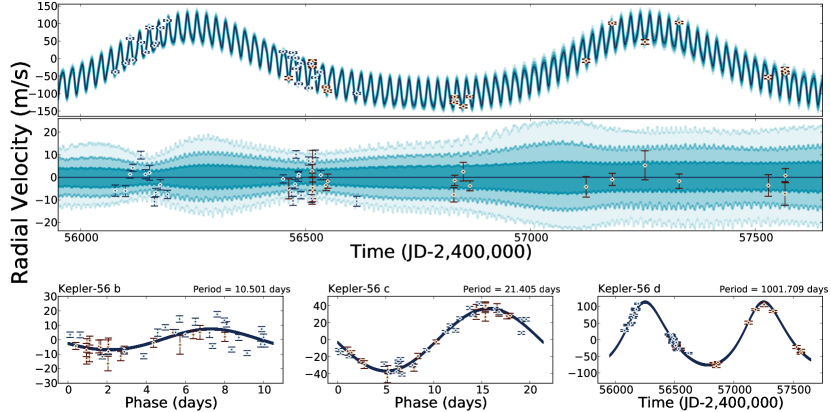
Figure 1.— A suite of results from our MCMC fit. (Top) Kepler-56  RV data – with HIRES points in red and those of HARPS in navy – together with a curve whose gradient represents the differing confidence levels of MCMC’s results, with the darkest navy representing the median fit and lighter shades corresponding to the 1, 2, and 3$\sigma$ uncertainties on the RV of the star as a function of time. (Middle) Identical to Panel 1, save that each data point and confidence curve has been subtracted by the median fit RV in order to show the data residuals and uncertainty as a function of time. (Lower left) Individual, phase folded RV contribution of Kepler-56 b to the system’s total RV. The contributions of the other two planets are subtracted from the HARPS and HIRES data displayed on the plot for visualization purposes. (Lower middle) The phase folded version of the lower left plot for Kepler-56 c with the signals from the other two planets removed for visualization purposes. (Lower right) Kepler-56 d’s individual, non-phase folded RV contribution, again with the other two planets removed.

For Kepler-56 d itself, we return a Doppler semiamplitude of 95.21 $\pm$ 1.84 m s^-1, corresponding to a minimum mass of $5.61\pm 0.38$ M${}_{\textrm{Jup}}$ ($1784\pm 120$ M_⊕). We also measure a period of $1002\pm 5$ days, an eccentricity of $0.20\pm 0.01$, and a semimajor axis of $2.16\pm 0.08$ AU.

4.1. Limits on a Fourth Planet

A fourth planet beyond the orbit of Kepler-56 d, if it exists, could be observable through the detection of a long-term trend in the data. Given our three-year baseline of observations, we can place limits on the presence of such an outer companion. From our emcee results, we find a long-term RV acceleration of $-0.25\pm 0.32$ m s^-1 yr^-1. The $95^{th}$ percentile value of the emcee posterior probability distribution for $\dot{\gamma}$ provides an upper limit on acceleration from a fourth planet of 0.80 m s^-1 yr^-1.

From Montet et al. (2014), we know the maximum trend caused by a planetary companion on a circular orbit is

$$\dot{\gamma}=(6.57\textrm{m s${}^{-1}$ yr${}^{-1}$})\bigg{(}\frac{m_{p}\sin i}{M_{J}}\bigg{)}\bigg{(}\frac{a}{5\textrm{AU}}\bigg{)}^{-2},$$ (5)

where $m_{p}$ is the mass of the planet, $M_{J}$ the mass of Jupiter, and $a$ the orbital semimajor axis. From this, we can place limits on the presence of outer companions with $m\sin i$ larger than $0.49M_{J}$ at 10 AU and $1.95M_{J}$ at 20 AU; such companions must be at particular points in their orbits or at low inclination in order to evade RV detection.

At $V\simeq 13$ mag, Kepler-56 falls just within Gaia’s bright-star limit (Perryman et al., 2014). A fourth planet’s acceleration on Kepler-56 in Gaia astrometry might be detectable at the level of 10-20 $\mu$as/yr² over the course of the mission. Averaging over flat priors for orbital angles and eccentricity, at the nominal distance of Kepler-56 ($d\sim 850$ pc), Gaia could in principle detect curvature due to orbital motion of a companion of $\gtrsim 20$ M_J at 10 AU or $\gtrsim 80$ M_J at 20 AU. These values in Equation 5 return, at the lowest, an acceleration of 32.85 m s^-1 yr^-1. This is much higher than the limits returned by our fit, suggesting that, save for face-on orbits, Gaia will be less helpful than continued RV observation in placing further limits on a fourth planet.

A fourth planet in a near-resonant orbit with Kepler-56 d could masquerade as a single eccentric planet, as described by Anglada-Escudé et al. (2010). However, we find the probability of this scenario to be low. Re-running our emcee fit with the outer planet’s eccentricity fixed at 0 leads to decreased likelihoods for the fit as a whole, and we do not detect any long-term structure in the residuals. However, our observations do not have the time resolution necessary to make a definitive assertion on this effect. Complete phase coverage of Kepler-56 d is needed to answer this question.

5. Discussion

5.1. Comparison to Previous Work

Our research supports that of Huber et al. (2013) in finding strong evidence for a massive, non-transiting exoplanet in the Kepler-56 system. Now that our observations span a full Kepler-56 d orbit, we can compare our results with the projections from Huber et al. (2013), who predicted that both the planetary obliquity and long-term RV trend could both be broadly explained by a non-transiting companion with a period of $900$ days and mass $3.3$ M${}_{\textrm{Jup}}$.

Both our minimum mass and period are similar to the representative values listed by Huber et al. (2013). Kepler-56 d’s minimum mass could be commensurate with that of a giant planet or a brown dwarf (for inclinations below 30 degrees). This could have implications for the near 2:1 resonance of the inner planets’ orbits, as well as for the misalignment of their orbital plane with that of Kepler-56 ’s rotation. Indeed, Li et al. (2014) simulated several scenarios and found a higher probability of the observed misalignment being of a dynamical origin (e.g. Fabrycky & Tremaine 2007) than from migration of the bodies in a tilted protoplanetary disk (e.g. Bate et al. 2010) or through angular momentum transport in the star itself that led to an apparent misalignment, even if the system was originally aligned (Rogers et al. 2012).

While Kepler-56 d is a possible source of dynamical perturbation, Gratia & Fabrycky (2016; submitted) simulate the scattering of two giant outer planets and find scattering between a system of three outer planets is required to excite the two inner planets of the system to inclinations similar to those observed in the data while preserving coplanarity. These additional planets, if real, must be scattered to large orbital separations or ejected entirely to evade detection by our RV observations.

5.2. The Effect of Kepler-56 d on Transits of the Inner Planets

Huber et al. (2013) inferred masses of the system’s inner planets by dynamically modeling their transits, ignoring possible perturbations from the third, outer planet. We verify that this is a reasonable assumption by checking two effects that may be significant: a tidal term corresponding to the change in the gravitational potential as Kepler-56 d completes its orbit, and a Roemer delay as the distance to the inner planets and host star vary over the orbit of the outer planet.

Following Equations 25-27 of Agol et al. (2005), the tidal effects would cause, over a long time baseline, the transits of an inner planet with mass $m_{1}$ and period $P_{1}$ to be perturbed with a standard deviation

$$\sigma=\frac{3\beta e_{2}}{\sqrt{2}(1-e_{2}^{2})^{3/2}}\bigg{[}1-\frac{3}{16}e_{2}^{2}-\frac{47}{1296}e_{2}^{4}-\frac{413}{27648}e^{6}_{2}\bigg{]}^{1/2},$$ (6)

where $e_{2}$ is the eccentricity of the outer planet and

$$\beta=\frac{m_{2}}{2\pi(m_{0}+m_{1})}\frac{P_{1}^{2}}{P_{2}}.$$ (7)

Here, $m_{2}$ is the mass of the outer planet with orbital period $P_{2}$, and $m_{0}$ the mass of the host star.

For the values in Table 2 for our system, we find perturbations in the time of transit on the order of four seconds for Kepler-56 b and sixteen seconds for Kepler-56 c. Given that the precision in the measurement of times of transit of these planets is typically tens of minutes, we do not expect these perturbations to affect, or be noticeable in, the measured times of transit.

The light travel time, or Roemer, delay is the result of changes in the physical distance between the observer and the host star due to the orbit of the outer body. Following Equations 6 and 7 of Rappaport et al. (2013), its magnitude is bounded such that

$$A_{R}\leq\frac{G^{1/3}}{c(2\pi)^{2/3}}P_{2}^{2/3}\bigg{[}\frac{m_{2}\sin i_{2}}{(m_{0}+m_{1}+m_{2})^{2/3}}\bigg{]},$$ (8)

where $G$ is Newton’s constant, $c$ the speed of light, and all other terms retain their meaning from the previous equation. Inserting values from Table 2 again, we find an expected light travel time signal not to exceed 5 seconds, significantly smaller than the observed uncertainties, so we do not expect Kepler-56 d to affect the orbits of the inner planets in any observable way.

5.3. Alternative Methods of Measuring Kepler-56 d

From our model, we measure a time of transit for Kepler-56 d of BJD-$2,400,000=56,450\pm 7$ days. Thus, if the planet transits the star, we would expect to detect a single transit in the Kepler dataset that is visible by eye, but do not observe one in this window. As we know the posterior distribution of allowed times of transit, we can determine the probability the planet transited during a data gap. In Quarters 6 and 7, there are four data gaps larger than 12 hours in which a transit could reside. Together, these gaps represent 1.7% of the mass of the posterior distribution of the time of central transit. The transit duration allows us to place even tighter constraints. If Kepler-56 d transited with an impact parameter $b=0$, the transit would have a duration of 3.1 days. As none of the gaps are longer than 20 hours in duration, we can additionally rule out any transits with $b<0.95$. By again integrating over the posterior distribution but accounting for the nonzero transit duration, assuming a flat distribution in impact parameter, we find that only 0.07% of allowed transits fall fully inside a data gap. If Kepler-56 d were to transit, there is a 99.93% proabability it would be observable in the Kepler data. Given this low probability and the a priori small transit probability for a companion on a $\sim 1000$ day period, it is likely this companion is non-transiting. We note that non-transiting does not necessarily imply non-coplanar with the inner planets, as the transit probability decreases with increasing semimajor axis (Borucki & Summers, 1984).

Having measured the minimum mass ($m\sin i$) and orbital semimajor axis ($a$) of Kepler-56 d, we can consider the possibility that the Gaia astrometric mission would be able to constrain its inclination. For lower (more face-on) inclinations, the planet will have a higher mass and the center of mass of the system will move closer to the planet. Additionally, the astrometric orbit will change shape on the sky, with more face-on inclinations appearing more circular throughout an orbit.

Given the distance to the system ($d\sim 850$ pc) and the inferred semimajor axis $2.13\pm 0.07$ AU, the orbit of Kepler-56 d has a projected semimajor axis on the sky of $\sim 2.5$ mas. From the mass ratio between the planet and star, we then expect an astrometric signal with a semiamplitude of $11\sin^{-1}\mu$as. Perryman et al. (2014) determined that Gaia will detect planets with astrometric signatures larger than $68\mu$as for stars as bright as Kepler-56, meaning this planet would evade detection at all except the lowest inclinations. However, given that the Gaia data can be combined with the prior information about the orbit of Kepler-56 d from RVs, it may be possible that the planet will be detected at slightly lower inclinations. Regardless, the prospects of a robust determination of the outer planet’s complete set of orbital parameters from Gaia appear unlikely.

Facilities: Keck:I (HIRES), TNG (HARPS-N)

6. Summary

Kepler-56, a red giant targeted in the telescope’s primary mission, has a massive, non-transiting companion detected through radial velocities. This star is one of only a few red giants known to have transiting planets, and these planets orbit with a nearly 2:1 period ratio on a plane misaligned relative to the spin of their host star. The presence of another body in the system was first detected by Huber et al. (2013) with observations from Keck/HIRES; we follow them up with subsequent observations from HIRES and HARPS-North at TNG. Incorporating these new data, we model the RV curve for a three-planet system. Our results confirm the existence of Kepler-56 d, with a period of $1002\pm 5$ days and a minimum mass of $5.61\pm 0.38$ M${}_{\textrm{Jup}}$. We also return an upper limit of acceleration from a possible fourth planet of 0.80 m s^-1 yr^-1 at 95% confidence, severely restricting the possibility of the existence of other giant planets within $\sim 20$ AU. We find that Kepler-56 d should not be detectable through its dynamical effect on the transits of the two inner planets, but for sufficiently face-on (more massive) orbits could be detectable through Gaia observations of its astrometric wobble.

References

- Agol et al. (2005) Agol, E., Steffen, J., Sari, R., & Clarkson, W. 2005, MNRAS, 359, 567
- Anglada-Escudé et al. (2010) Anglada-Escudé, G., López-Morales, M., & Chambers, J. E. 2010, ApJ, 709, 168
- Baranne et al. (1996) Baranne, A., Queloz, D., Mayor, M., et al. 1996, A&AS, 119, 373
- Barclay et al. (2015) Barclay, T., Quintana, E. V., Adams, F. C., et al. 2015, ApJ, 809, 7
- Batalha et al. (2010) Batalha, N. M., Borucki, W. J., Koch, D. G., et al. 2010, ApJ, 713, L109
- Batalha et al. (2013) Batalha, N. M., Rowe, J. F., Bryson, S. T., et al. 2013, ApJS, 204, 24
- Bate et al. (2010) Bate, M. R., Lodato, G., & Pringle, J. E. 2010, MNRAS, 401, 1505
- Borucki & Summers (1984) Borucki, W. J., & Summers, A. L. 1984, Icarus, 58, 121
- Borucki et al. (2010) Borucki, W. J., Koch, D., Basri, G., et al. 2010, Science, 327, 977
- Borucki et al. (2011) Borucki, W. J., Koch, D. G., Basri, G., et al. 2011, ApJ, 736, 19
- Burke et al. (2014) Burke, C. J., Bryson, S. T., Mullally, F., et al. 2014, ApJS, 210, 19
- Butler et al. (1996) Butler, R. P., Marcy, G. W., Williams, E., et al. 1996, PASP, 108, 500
- Ciceri et al. (2015) Ciceri, S., Lillo-Box, J., Southworth, J., et al. 2015, A&A, 573, L5
- Cosentino et al. (2012) Cosentino, R., Lovis, C., Pepe, F., et al. 2012, in Proc. SPIE, Vol. 8446, Ground-based and Airborne Instrumentation for Astronomy IV, 84461V
- Eastman et al. (2013) Eastman, J., Gaudi, B. S., & Agol, E. 2013, PASP, 125, 83
- Fabrycky & Tremaine (2007) Fabrycky, D., & Tremaine, S. 2007, ApJ, 669, 1298
- Ford et al. (2011) Ford, E. B., Rowe, J. F., Fabrycky, D. C., et al. 2011, ApJS, 197, 2
- Ford et al. (2012) Ford, E. B., Fabrycky, D. C., Steffen, J. H., et al. 2012, ApJ, 750, 113
- Foreman-Mackey et al. (2013) Foreman-Mackey, D., Hogg, D. W., Lang, D., & Goodman, J. 2013, PASP, 125, 306
- Goodman & Weare (2010) Goodman, J., & Weare, J. 2010, Communications in Applied Mathematics and Computational Science, 5, 65
- Grunblatt et al. (2016) Grunblatt, S. K., Huber, D., Gaidos, E. J., et al. 2016, ArXiv e-prints, arXiv:1606.05818
- Howard et al. (2010) Howard, A. W., Johnson, J. A., Marcy, G. W., et al. 2010, ApJ, 721, 1467
- Huber et al. (2013) Huber, D., Carter, J. A., Barbieri, M., et al. 2013, Science, 342, 331
- Johnson (2008) Johnson, J. A. 2008, in Astronomical Society of the Pacific Conference Series, Vol. 398, Extreme Solar Systems, ed. D. Fischer, F. A. Rasio, S. E. Thorsett, & A. Wolszczan, 59
- Kipping et al. (2016) Kipping, D. M., Torres, G., Henze, C., et al. 2016, ApJ, 820, 112
- Kostov et al. (2015) Kostov, V. B., Orosz, J. A., Welsh, W. F., et al. 2015, ArXiv e-prints, arXiv:1512.00189
- Lehmann-Filhés (1894) Lehmann-Filhés, R. 1894, Astronomische Nachrichten, 136, 17
- Li et al. (2014) Li, G., Naoz, S., Valsecchi, F., Johnson, J. A., & Rasio, F. A. 2014, ApJ, 794, 131
- Lillo-Box et al. (2014) Lillo-Box, J., Barrado, D., Moya, A., et al. 2014, A&A, 562, A109
- Montet et al. (2014) Montet, B. T., Crepp, J. R., Johnson, J. A., Howard, A. W., & Marcy, G. W. 2014, ApJ, 781, 28
- Mullally et al. (2015) Mullally, F., Coughlin, J. L., Thompson, S. E., et al. 2015, ApJS, 217, 31
- Pepe et al. (2002) Pepe, F., Mayor, M., Rupprecht, G., et al. 2002, The Messenger, 110, 9
- Pepper et al. (2016) Pepper, J., Rodriguez, J. E., Collins, K. A., et al. 2016, ArXiv e-prints, arXiv:1607.01755
- Perryman et al. (2014) Perryman, M., Hartman, J., Bakos, G. Á., & Lindegren, L. 2014, ApJ, 797, 14
- Quinn et al. (2015) Quinn, S. N., White, T. R., Latham, D. W., et al. 2015, ApJ, 803, 49
- Rappaport et al. (2013) Rappaport, S., Deck, K., Levine, A., et al. 2013, ApJ, 768, 33
- Rogers et al. (2012) Rogers, T. M., Lin, D. N. C., & Lau, H. H. B. 2012, ApJ, 758, L6
- Rowe et al. (2015) Rowe, J. F., Coughlin, J. L., Antoci, V., et al. 2015, ApJS, 217, 16
- Steffen et al. (2012) Steffen, J. H., Ford, E. B., Rowe, J. F., et al. 2012, ApJ, 756, 186
- Steffen et al. (2013) Steffen, J. H., Fabrycky, D. C., Agol, E., et al. 2013, MNRAS, 428, 1077
- Valenti et al. (1995) Valenti, J. A., Butler, R. P., & Marcy, G. W. 1995, PASP, 107, 966
- Van Eylen et al. (2016) Van Eylen, V., Albrecht, S., Gandolfi, D., et al. 2016, ArXiv e-prints, arXiv:1605.09180
- Vogt et al. (1994) Vogt, S. S., Allen, S. L., Bigelow, B. C., et al. 1994, in Society of Photo-Optical Instrumentation Engineers (SPIE) Conference Series, Vol. 2198, Society of Photo-Optical Instrumentation Engineers (SPIE) Conference Series, ed. D. L. Crawford & E. R. Craine, 362