Fast Backprojection Techniques for High Resolution Tomography

Abstract

Fast image reconstruction techniques are becoming important with the increasing number of scientific cases in high resolution micro and nano tomography. The processing of the large scale three-dimensional data demands new mathematical tools for the tomographic reconstruction task because of the big computational complexity of most current algorithms as the sizes of tomographic data grow with the development of more powerful acquisition hardware and more refined scientific needs. In the present paper we propose a new fast back-projection operator for the processing of tomographic data and compare it against other fast reconstruction techniques.

1 Introduction

Tomographic imaging is a very powerful instrument of non-destructive research and control of the internal structure of non-opaque objects. An important branch of tomographic techniques is transmission tomography, which can be used at nano, micro and macro resolution levels. For further consideration we describe in general the basic principles of transmission tomography from parallel rays, and define some notations.

Physically, all types of transmission tomography are based on registering the energy loss or/and intensity loss of the incoming electromagnetic wave (x-rays for instance), after passing through the object under investigation also referred to here as sample). In our case, we consider that x-rays generated from a synchrotron light source hit the object under investigation determining a projection image (also referred as frame) at a ccd (charge coupled device) camera. A typical dataset is shown in Figure 1.A, where a high-resolution frame $P$ gathered using the x-rays source is shown, with dimensions $2048\times 2048$. After half-rotation of the sample on the rotation axis, we obtain a cubic dataset as shown in Figure 1.B. Each slice of this dataset give us an image, which is called sinogram, and that will be used as input to an appropriate inversion algorithm in order to reconstruct the slice of the sample.

Figure 1: (A) Projection (or frame) for a cylindrical sample obtained with a ccd camera (B) Three-dimensional representation of the measured data: $P$ is the measured frame and $G$ is the sinogram image at a given row of the area detector.

We introduce the cartesian coordinate system in the plane of a given slice of the object. Let the function $f({\bm{x}})\in U$ be the feature function, i.e., a function which depends on the internal structure of the object in the plane of the slice and which defines the linear absorption coefficient of the sample. Set $U$, referred to here as the feature space, is a Schwartz space $\mathcal{S}(\mathbb{R}^{2})$.

A given frame (see Figure 1.A) represents the integral of $f({\bm{x}})$ over straight lines passing through the sample and perpendicular to the detector’s plane. One row of each of these frame images contains the integrals relevant to a slice of the object, and orthogonal to the rotation axis. Let us introduce an axis $t$ over the detector’s row. It is clear that for each angle $\theta$ (see Figure 2), such a row is mathematically determined by

$$g(\theta,t)\equiv g_{\theta}(t)=\int\limits_{L(\theta,t)}f({\bm{x}})\mathrm{d}s=\int\limits_{\mathbb{R}^{2}}f({\bm{x}})\delta({\bm{x}}\cdot{\bm{\xi}}_{\theta}-t)\mathrm{d}\bm{x},$$ (1.1)

where $L(\theta,t)$ is a straight line defining the x-ray path,

$$L{(\theta,t)}=\big{\{}{\bm{x}}\in\mathbb{R}^{2}:{\bm{x}}\cdot{\bm{\xi}}_{\theta}=t\big{\}},\ \ \ {\bm{\xi}}_{\theta}=(\cos\theta,\sin\theta)^{T}.$$ (1.2)

From (1.1) we have a linear operator acting on the feature function $f$, i.e., $\mathscr{R}\colon f\in U\mapsto g\in V$, which is called the Radon transform. Space $V$ is the Schwartz space $\mathcal{S}(\mathbb{R}_{+}\times[0,\pi])$. The operator $\mathscr{B}\colon V\to U$ defined as

$$b({\bm{x}})=\mathscr{B}g({\bm{x}})=\int_{[0,\pi]}g({\bm{x}}\cdot{\bm{\xi}}_{\theta},\theta)\mathrm{d}\theta,$$ (1.3)

is defined as the backprojection operator, and is the adjoint of $\mathscr{R}$ in the following sense

$$\int\limits_{\mathbb{R}_{+}\times[0,\pi]}\mathscr{R}f(t,\theta)g(t,\theta)\mathrm{d}t\mathrm{d}\theta=\int\limits_{\mathbb{R}^{2}}f({\bm{x}})\mathscr{B}g({\bm{x}})\mathrm{d}{\bm{x}},$$ (1.4)

More about the theory of the integral operators $\{\mathscr{R},\mathscr{B}\}$ can be found on [1, 2, 3, 4].

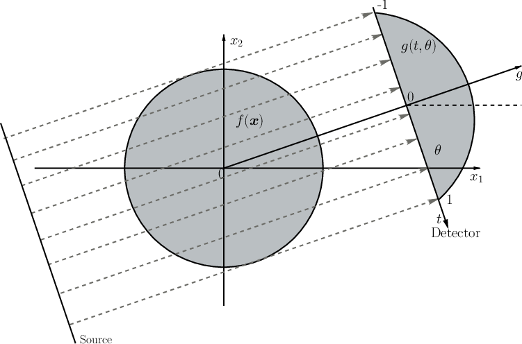
Figure 2: Geometry of incoming x-rays for parallel tomography.

At this point, it is convenient to introduce some notations. We first introduce the notations for the representation of feature function $f:\mathbb{R}^{2}\to\mathbb{R}$ in different coordinate systems, and their respective jacobians:

(a)

Prüfer coordinates (see [5]): ${\bm{x}}=p(\mu){\bm{\xi}}_{\theta}$, $\mathrm{d}{\bm{x}}=|p^{\prime}(\mu)p(\mu)|\mathrm{d}\mu\mathrm{d}\theta$. The representation is denoted by $[f]_{\mathsf{Pr}}(\mu,\theta)$. Function $p$ will always be well defined within the context by special notation as follows;

(b)

Log-polar coordinates: particular case of Prüfer coordinates when $p(\mu)=e^{\mu}$. Here, $\mathrm{d}{\bm{x}}=e^{2\mu}\mathrm{d}\mu\mathrm{d}\theta$. The representation is denoted by $[f]_{\mathsf{L}}(\mu,\theta)$;

(c)

Semi-polar coordinates: particular case of Prüfer coordinates when $p(\mu)=\mu$. Here, $\mathrm{d}{\bm{x}}=\mu\mathrm{d}\mu\mathrm{d}\theta$. The representation is denoted by $[f]_{\mathsf{P}}(\mu,\theta)$.

(d)

Sinogram coordinates are similar to the semi-polar coordinates and, in fact, can be obtained by flipping the angles $\theta\in[\pi,2\pi)$ to the negative part of the $t$-axis , so that $t\in[-1,1]$.

Using the above notation, function $g$ in (1.1) can be written as $[g]_{\sf P}(t,\theta)$ in order to indicate semi-polar coordinates. An example, using the well-known Shepp-Logan phantom [6] is presented on Figure 3. The sinogram of the Shepp-logan feature function $f$ is presented in the sinogram coordinate system mentioned above.

(a)	(b)
(c)	(d)

Figure 3: (a) Shepp-Logan feature function $f(x)$ and his associated sinograms, in different coordinate systems: (b) Semi-polar coordinates $[g]_{\sf s}$, (c) Polar coordinates $[g]_{\sf P}$ and (d) Log-polar coordinates $[g]_{\sf L}$.

Our goal in the present paper is to present a fast method for the computation of the backprojection image $b\in U$ for a given sinogram $g\in V$. The computation of the tomographic image from sinogram data depends on the backprojection operator $\mathscr{B}$, which bears the major computational cost of reconstruction methods: $O(N^{3})$ for images with $N^{2}$ pixels and $N$ projections.

For a high-resolution tomographic synchrotron experiment, the amount of data at a micro-tomography setup is considerably large for today’s computational standards, mainly because of this asymptotic floating point operations (flops) count. Indeed, at the Brazilian National Synchrotron Light Source (lnls) one wishes to obtain $2048$ reconstructions images with $2048\times 2048$ pixels from datasets having $3200\times 2048$ points, or possibly more. Therefore, implementation of $\mathscr{B}$ represent the main bottleneck of the reconstruction process. If certain useful mathematical properties of $\mathscr{B}$ are exploited, the computational effort can be significantly reduced to $O(N^{2}\log N)$ flops [7, 8].

Several techniques were developed aiming at a reduction to $O(N^{2}\log N)$ flops for computing $\mathscr{B}$. One approach was established in [9], where the computation of $\mathscr{B}g$ is performed after a change from cartesian to log-polar coordinates in the data. This approach leads to a convolution, which is computable through Fast Fourier Transform (fft) algorithms. Although elegant, the methods suffer from the ill-conditioning of the Log-polar transform at the “fovea”. Nevertheless, it is possible to translate the fovea to different regions of the cartesian plane, in order to enclose the reconstruction region. This leads to the concept of partial-backprojection which can be easily implemented in a parallel form. Other methods for fast computation of $\mathscr{B}$ were presented in [10, 11, 12, 13], using a divide and conquer strategy based on hierarchical decompositions of the full backprojection which are simpler than the full backprojection. Hierarchical decompositions can be created both in the image [12] or in the data [10, 11]. Yet another approach is based on Non-uniform Fast Fourier Transform (nfft) algorithms (see [12, 14, 15]) and the so-called Fourier Slice Theorem ([2, 16]. In this paper, we propose another fast method for the computation of $\mathscr{B}g$, also based on Fourier transforms. We claim that the backprojection of $g\in V$ can be easily done by filtering the lines of the $\tilde{g}$ one by one, where $\tilde{g}$ is the polar representation of $g$ in $S_{+}=\mathbb{R}\times[0,2\pi]$.

This manuscript is organized as follows: Section 2 presents a discussion of low-complexity algorithms for the computation of $\mathscr{B}$. Our low-complexity formula is presented in Section 3 and a discussion of the implementation is presented in Section 5. Further comparison of all algorithms is presented in Section 7 and a discussion of the results is shown in Section 8.

Remark: In this manuscript we use the the integral operator, sometimes with $\mathrm{d}x$ placed before the integrand, as it is more convenient to make explicit the variables being considered. Whenever the integrand is short, we adopt the classic notation $\int f(x)\mathrm{d}x$.

2 Class of Algorithms for the Backprojection

Let $g\in V$ be a given sinogram. A naïve implementation of the typical backprojection formula (1.4) has to be done using nested loops. Indeed, for each pixel $x$ lying on a predefined meshgrid within the square $\|x\|_{\infty}\leq 1$, the approximation of $b(x)=\mathscr{B}g(x)$ is given by

$$b(x)\approx\Delta\theta\sum_{k=1}^{N_{\theta}}g(x\cdot\xi_{\theta_{k}},\theta_{k}).$$ (2.1)

It is easy to realize that the above approximation has a computational cost of $O(N_{\theta})$ for each pixel $x$, where $N_{\theta}$ is the total number of sampled angles. For a high resolution frame (see Figure 1.A), a linear interpolation for $x\cdot\xi_{\theta}$ on the grid of $-1\leq t\leq 1$ is usually precise enough. Assuming that $b$ is represented by a square image of order $N\times N$, the total cost for computing the final backprojected image $b$ is $O(N^{2}N_{\theta})$. In practice, $N_{\theta}$ has almost the same magnitude of $N$, and thus we can state that the asymptotic cost to obtain $b$ is $O(N^{3})$. Such an algorithm is impractical for high-resolution images.

There are at least three other types of backprojection algorithms which can dramatically reduce the computing time of the backprojected image $b$, for large datasets:

(i)

A fast slant-stack based approach [17] was proposed by Averbuch et al. Although this is an elegant and fast approach, it will not be covered in this manuscript;

(ii)

Hierarchical decomposition [10, 12, 11]: Two different approaches that apply the divide-and conquer paradigm to the backprojection computation, splitting it recursively into smaller and simpler subproblems;

(iii)

NFFT [18]: The Fourier Slice Theorem sets the Fourier Transform as bridge between the Radon Transform $\mathcal{R}f(\theta,t)$ and the original image $f$. However, tomographic data does not provide an evenly distributed sampling of the Fourier space, as required by traditional fft techniques (see [19]). Use of this Fourier approach was enabled by research on nfft algorithms (see [12, 14, 15]);

(iv)

Anderson’s formula [9]: Such a formula is obtained with an appropriate change of variables on the classical equation of the backprojection formula (1.4). The main idea is to convolve the sinogram in log-polar coordinates with an ideal kernel using fft algorithms.

In this paper, we focus mainly on the description of our algorithm and algorithm (iii).

2.1 Log-polar backprojection

A fast method for obtaining the backprojection was derived by Andersson [9]. His approach is based on a representation of the Backprojection/Radon transform as a convolution, by casting the computation in a log-polar coordinate system. In this section we propose a different proof for his formula.

Let $g=\mathscr{R}f$ be a given sinogram, i.e., the Radon transform of a compactly supported function $f$. Using the coordinate system notation of the previous section, where $[\cdot]_{\sf L}$ denotes the log-polar representation of some function, the main formula of the log-polar backprojection is written as

$$[\mathscr{B}g]_{\mathsf{L}}(\rho,\theta)=[g]_{\mathsf{L}}*[K]_{\mathsf{L}}\ (\rho,\theta),$$ (2.2)

where $*$ stands for the two-dimensional convolution, and $K$ is the convolution Kernel

$$[K]_{\mathsf{L}}(\rho,\theta)=\delta(1-e^{\rho}\cos\theta).$$ (2.3)

Using above formula and the convolution theorem, we obtain

$$[\mathscr{B}g]_{\mathsf{L}}=\mathcal{F}^{-1}\big{(}\mathcal{F}[g]_{\mathsf{L}}\cdot\mathcal{F}[K]_{\mathsf{L}}\big{)}.$$ (2.4)

Let us give a simple proof of the above equation, assuming that $f$ lies in a Schwartz space $\mathcal{S}(\mathbb{R}^{2})$, and $g\in\mathcal{S}(\mathbb{R}_{+}\times[-\pi,\pi])$.

Proof: We start with the integral representation of the backprojection operator, given in (A.7) (See Appendix A). Now, formula (2.2) is derived in four steps:

(a)

Changing the integral (A.7) from cartesian coordinates $\bm{y}\in\mathbb{R}^{2}$ to Prüfer coordinates, i.e., $\bm{y}\equiv\bm{y}_{\mu,\theta}=p(\mu)\bm{\xi}_{\phi}$ we get $\mathrm{d}\bm{y}=|p^{\prime}(\mu)p(\mu)|\mathrm{d}\mu\mathrm{d}\theta$ and

$$\mathscr{B}g(\bm{x}_{\rho,\theta})=\int_{S_{+}}g(\bm{y}_{\mu,\phi})\delta\left(\kappa_{\bm{x}_{\rho,\theta}}(\bm{y}_{\mu,\phi})\right)|p^{\prime}(\mu)p(\mu)|\mathrm{d}\mu\mathrm{d}\phi$$ (2.5)

(b)

The support of the Delta distribution in (2.5) is

$$\kappa_{\bm{x}_{\rho,\theta}}(\bm{y}_{\mu,\phi})=p(\mu)^{2}\left[1-\frac{p(\rho)}{p(\mu)}\bm{\xi}_{\phi}\cdot\bm{\xi}_{\theta}\right]=p(\mu)^{2}\left[1-\frac{p(\rho)}{p(\mu)}\cos(\phi-\theta)\right]$$ (2.6)

(c)

Let $[\cdot]_{\mathsf{Pr}}$ be the representation in Prüfer coordinates. From (2.6) and (2.5) we arrive at

$$[\mathscr{B}g]_{\mathsf{Pr}}(\rho,\theta)\\ {}=\displaystyle\int_{S_{+}}[g]_{\mathsf{G}}(\mu,\phi)\delta\left(p(\mu)^{2}\left[1-\frac{p(\rho)}{p(\mu)}\cos(\phi-\theta)\right]\right)|p^{\prime}(\mu)p(\mu)|\mathrm{d}\mu\mathrm{d}\phi\\ {}=\displaystyle\int_{S_{+}}[g]_{\mathsf{G}}(\mu,\phi)\delta\left(1-\frac{p(\rho)}{p(\mu)}\cos(\phi-\theta)\right)\frac{|p^{\prime}(\mu)p(\mu)|}{p(\mu)^{2}}\mathrm{d}\mu\mathrm{d}\phi$$ (2.7)

where $S_{+}=\mathbb{R}_{+}\times[-\pi,\pi]$

(d)

A convolution is obtained in (2.7) only if $p$ is such that $p(\rho)=p(\mu)p(\rho-\mu)$, which in turn implies that $p$ is an exponential function. Hence, Prüfer coordinates reduce to log-polar coordinates, which we denote by $[\cdot]_{\mathsf{L}}$. Finally, we obtain

$$[\mathscr{B}g]_{\mathsf{L}}(\rho,\theta)=\int_{S_{+}}[g]_{\mathsf{L}}(\mu,\phi)\delta\left(1-e^{\rho-\mu}\cos(\phi-\theta)\right)\mathrm{d}\mu\mathrm{d}\phi$$ (2.8)

which is the final convolution formula. ∎

3 Back-projection Slice Theorem

Although Anderson’s approach is asymptotically fast, it has a few drawbacks. Firstly, the gain of speed using Fourier transforms to compute the convolution is reduced with forward/backward log-polar transformations. Also, these interpolations can produce errors, especially near the origin, due to a strong non-uniformity of the log-polar mesh in that region. To avoid these factors, another approach for the calculation of the backprojection operator can be used. This approach is based on the following theorem:

Theorem (Backprojection Slice Theorem (BST)).

Let $g=g(t,\theta)\in V$ a given sinogram and $\widehat{\cdot}$ denotes the Fourier transform operation. It follows that the backprojection $\mathscr{B}$ satisfies

$$\widehat{\mathscr{B}g}(\sigma\xi_{\theta})=\frac{\hat{g}(\sigma,\theta)}{\sigma}$$ (3.1)

with $\sigma>0\in\mathbb{R}$ and $\theta\in[0,2\pi]$.

Proof.

Using the sifting property of the $\delta$-distribution, the backprojection (1.3) can be presented in the following form

$$\mathscr{B}g(x)=\int_{0}^{\pi}g(x\cdot\xi_{\theta},\theta)\mathrm{d}\theta=\int_{0}^{\pi}\int_{\mathbb{R}}g(t,\theta)\delta(t-x\cdot\xi_{\theta})\mathrm{d}t\mathrm{d}\theta$$

Considering the two-dimensional Fourier transform of $\mathscr{B}g$, i.e., $\mathcal{F}\colon\mathscr{B}g\mapsto\widehat{\mathscr{B}g}$ and using representation (A.7) (see Appendix),

$$\widehat{\mathscr{B}g}(\omega)=\int_{\mathbb{R}^{2}}\mathscr{B}g(x)e^{-i\omega\cdot x}\mathrm{d}x=\int_{\mathbb{R}^{2}}\!\!\!\mathrm{d}x\int_{\mathbb{R}^{2}}\!\!\!\mathrm{d}y\ [g]_{\mathsf{c}}(y)\delta\left(y\cdot(y-x)\right)e^{-i\omega\cdot x}$$

$$=\int_{\mathbb{R}^{2}}\!\!\!\mathrm{d}y\ [g]_{\mathsf{c}}(y)\int_{\mathbb{R}^{2}}\!\!\!\mathrm{d}x\ \delta\left(y\cdot(y-x)\right)e^{-i\omega\cdot x}\equiv\int_{\mathbb{R}^{2}}\!\!\!\mathrm{d}y\ [g]_{\mathsf{c}}(y)\mathcal{T}(y,\omega)$$

where $y,\omega\in\mathbb{R}^{2}$ and

$$\mathcal{T}(y,\omega)=\int_{\mathbb{R}^{2}}\!\!\!\mathrm{d}x\ \delta\left(h_{y}(x)\right)e^{-i\omega\cdot x},\ \ \ \ h_{y}(x)=y\cdot(y-x)$$ (3.2)

Since the distribution (3.2) is supported in the set $h^{-1}_{y}(0)=\{x\in\mathbb{R}^{2}\colon h_{y}(x)=0\}$, it follows from (A.1) (See Appendix A) and $\nabla h_{y}=-y$ that

$$\mathcal{T}(y,\omega)=\frac{1}{\|{y}\|}\int_{h^{-1}_{{y}}(0)}e^{-i{\omega}\cdot{x}}\mathrm{d}s(x)=\int_{h^{-1}_{{y}}(0)}e^{-i{\omega}\cdot{x}(q)}\mathrm{d}q$$ (3.3)

The set $h^{-1}_{{y}}(0)$ determines a straight line passing through ${y}$ and with normal vector ${y}$. Thus, $h^{-1}_{{y}}(0)={y}+\mbox{span}\{S{y}\}$, being $S{y}\perp{y}$ and $S$ a $\frac{\pi}{2}$-rotation matrix. Therefore, ${x}(q)\in h^{-1}_{{x}}(0)$ is on the form ${x}(q)={y}+qS{y}$ and the integral in (3.3) can be written as:

$$\mathcal{T}({y},{\omega})=\int_{\mathbb{R}}e^{-i{\omega}\cdot[{y}+qS{y}]}\mathrm{d}q=e^{-i{\omega}\cdot{y}}\int_{\mathbb{R}}e^{-iq{\omega}\cdot(S{y})}\mathrm{d}q=e^{-i{\omega}\cdot{y}}\delta\left({\omega}\cdot S{y}\right)$$ (3.4)

Hence, the Fourier transform of $\mathscr{B}g$ becomes

$$\widehat{\mathscr{B}g}({\omega})=\int_{\mathbb{R}^{2}}[g]_{\mathsf{c}}({y})\delta\left({\omega}\cdot S{y}\right)e^{-i{\omega}\cdot{y}}\ \mathrm{d}{y}$$ (3.5)

For ${\omega}$ fixed, $\{{y}\in\mathbb{R}^{2}\colon{\omega}\cdot(S{y})=0\}=\mbox{span}\{{\omega}\}$, with $S$ aπ $\frac{\pi}{2}$-rotation matrix. Indeed, since $S{y}\perp{w}$ and $S{y}\perp{y}$, it follows ${\omega}\parallel{y}$. Once again, using the representation (A.1) (see Appendix A) for (3.5) we arrive at

$$\widehat{\mathscr{B}g}({\omega})=\int_{\mathbb{R}}\frac{[g]_{\mathsf{c}}(q{\omega})}{\|S{\omega}\|}e^{-i{\omega}\cdot(q{\omega})}\ \mathrm{d}s(\omega)$$ (3.6)

Since $\|S{\omega}\|=\|{\omega}\|$ and $\mathrm{d}s(\omega)=\|\omega\|dq$, we finally obtain

$$\widehat{\mathscr{B}g}({\omega})=\int_{\mathbb{R}}[g]_{\mathsf{c}}(q{\omega})e^{-iq\|{\omega}\|^{2}}\ \mathrm{d}q$$ (3.7)

From the above equation, the backprojection is a polar convolution. Indeed, switching the frequency domain to polar coordinates, i.e., ${\omega}=\sigma{\xi}_{\theta}$ (with $\sigma\in\mathbb{R}_{+}$ and $\theta\in[0,2\pi]$) we get

$$\widehat{\mathscr{B}g}(\sigma{\xi}_{\theta})=\int_{\mathbb{R}}[g]_{\mathsf{c}}(q\sigma{\xi}_{\theta})e^{-iq\|\sigma{\xi}_{\theta}\|^{2}}\mathrm{d}q=\int_{\mathbb{R}}\frac{[g]_{\mathsf{c}}(u{\xi}_{\theta})}{\sigma}e^{-iu\sigma}\mathrm{d}u.$$ (3.8)

Now, letting $[\cdot]_{\mathsf{s}}$ be the representation in semi-polar coordinates, it is true that $[g]_{\mathsf{c}}(u{\xi}_{\theta})=g(u,\theta)$ is the input sinogram $g(u,\theta)$. From (3.7) and (3.8), using polar coordinates

$$[\widehat{\mathcal{\mathscr{B}}g}]_{\sf p}(\sigma,\theta)=\widehat{\mathcal{\mathscr{B}}g}(\sigma{\xi}_{\theta})=\frac{1}{\sigma}\int_{\mathbb{R}}g(u,\theta)e^{-iu\sigma}\mathrm{d}u$$ (3.9)

Identity (3.9) is our backprojection-slice Theorem (3.1) for computing the operator $\mathscr{B}$. ∎

Indeed, at each radial line $\theta$ in the frequency domain, the two-dimensional Fourier transform of $\mathscr{B}$ equals the one-dimensional radial Fourier transform of the projection $g(t,\theta)$ multiplied by the kernel $1/\sigma$ for $\sigma>0$.

Remark 1: The mathematical proof outlined above provides a direct formula for the computation of a backprojected image, i.e., given a sinogram $g$, the explicit steps to compute the backprojection in the frequency polar coordinates results in formula (3.1). In practice, there are several iterative methods that depends explicitly on the computation of the backprojection of any sinogram. In the other hand, analytical formulas usually handle with the backprojection of a filtered sinogram, from where standard formulas like the filtered backprojection or the filter of the backprojection are established. To validate our backprojection result we remark the following items:

(i) It is a well known fact [1, 4, 2] that, for a given feature function $f\in U$, the following property holds

$$\mathscr{B}\mathscr{R}f(x)=(f*h)(x),\ \ \ \ h(x)=\frac{1}{\|x\|}$$ (3.10)

which, in the frequency domain, is written as (cartesian and polar representation, respectively)

$$\widehat{\mathscr{B}\mathscr{R}f}(w)=\hat{f}(w)\frac{1}{\|w\|}\ \ \ \Leftrightarrow\ \ \ \widehat{\mathscr{B}\mathscr{R}f}(\sigma\xi_{\theta})=\hat{f}(\sigma\xi_{\theta})\frac{1}{\sigma}$$ (3.11)

due to the fact that $\mathcal{F}\colon\frac{1}{\|x\|}\mapsto\frac{1}{\|w\|}$. Now, replacing the backprojection slice theorem (3.1) into (3.11), we obtain

$$\widehat{\mathscr{R}f}(\sigma\xi_{\theta})\frac{1}{\sigma}=\hat{f}(\sigma\xi_{\theta})\frac{1}{\sigma}\ \ \ \Rightarrow\ \ \ \widehat{\mathscr{R}f}(\sigma\xi_{\theta})=\hat{f}(\sigma\xi_{\theta})$$ (3.12)

which is the celebrated Fourier Slice-Theorem [3].

(ii) From the classical inversion of the Radon transform, i.e., the filtered-backprojection algorithm, it is true that

$$\mathscr{B}Fg(x)=f(x),\ \ \ g=\mathscr{R}f$$ (3.13)

where $F$ is a low-pass filtering operator, that is $\widehat{Fg}(\nu,\theta)=\hat{g}(\nu,\theta)|\nu|$, for $\nu\in\mathbb{R}$. In the polar frequency domain, (3.13) reads $\widehat{\mathscr{B}Fg}(\sigma\xi_{\theta})=\hat{f}(\sigma\xi_{\theta})$. From the backprojection slice Theorem (3.1), such equation becomes

$$\frac{1}{\sigma}\widehat{Fg}(\sigma\xi_{\theta})=\hat{f}(\sigma\xi_{\theta})\ \ \ \Rightarrow\ \ \ \frac{1}{\sigma}\hat{g}(\sigma\xi_{\theta})\sigma=\hat{f}(\sigma\xi_{\theta}),\ \ \ \ \sigma\in\mathbb{R}_{+}$$ (3.14)

Once again, the above equation yields the Fourier Slice-Theorem.

Remark 2: The dc-component of the Backprojection of some function $g$ lying in the sinogram space is defined by

$$\widehat{\mathscr{B}g}() = \int_{\mathbb{R}^{2}}\mathscr{B}g(x)\mathrm{d}x$$ (3.15)

$$= \int_{\mathbb{R}^{2}}\mathrm{d}x\int_{0}^{\pi}\mathrm{d}\theta\ g(x\cdot\xi_{\theta},\theta)$$ (3.16)

$$= \int_{0}^{\pi}\mathrm{d}\theta\int_{\mathbb{R}}\mathrm{d}t\int_{\mathbb{R}}\mathrm{d}s\ g(t,\theta)\equiv M$$ (3.17)

where we have used $\mathrm{d}x=\mathrm{d}t\mathrm{d}s$ to make explicit the change of variables from $x$ to $(t,s)$, being $s$ the variable along the direction $\xi_{\theta}^{\perp}$. The dc of an arbitrary $g\in V$ provide $M=\infty$. In this sense, $\widehat{\mathscr{B}g}$ behaves like a tempered distribution since $\mathscr{B}g$ lies in a Schwartz space, where the Fourier transform is an automorphism. Also, it is easy to note that

$$\frac{\hat{g}(\sigma,\theta)}{\sigma}=i\hat{h}(\sigma,\theta),\ \ h(t)=\int_{\infty}^{t}g(t,\theta)\mathrm{d}t$$ (3.18)

i.e., $h$ is a primitive of $g$. Hence, using (3.18) as $\sigma\to 0$, the limit of the ratio $\hat{g}(\sigma,\theta)/\sigma$ diverge in $\sigma=0$. Finally, bst formula can be easily applied for some $g\in V$ with a nonzero dc-component. In fact, setting $p(t,\theta)=g(t,\theta)-\hat{g}(0,\theta)$, it is true that $\hat{p}(0,\theta)=0$ and the backprojection of $g$ follows with $\mathscr{B}g(\bm{x})=\mathscr{B}p(\bm{x})+\hat{g}(0,\theta)$.

4 Analytical Examples

In this section, we provide two examples where the analytical computation of the backprojection operator is possible. This is important to validate further numerical simulations. The first example given is for a point source function, both in log-polar and cartesian coordinates. The second one, for a symmetrical circular function. In what follows, we consider that $g=g(t,\theta)$ is the Radon transform of $f=f(\bm{x})$, while $b=b(\bm{x})$ is the final backprojected image.

Example I: Following Andersson’s formula , the backprojection of any sinogram $g$ is written as a convolution in Log-polar coordinates

$$b(e^{\rho}\bm{\xi}_{\theta})=\mathscr{B}g(e^{\rho}\bm{\xi}_{\theta})=\int\mathrm{d}u\int\mathrm{d}\beta\ \ g(e^{u},\beta)\delta(1-e^{\rho-u}\cos(\theta-\beta))$$ (4.1)

It is a well known fact that the Radon transform of a single point source, located at $\bm{x}=\bm{a}$ is

$$f(\bm{x})=\delta(\bm{x}-\bm{a})\ \ \ \Rightarrow\ \ \ g(t,\theta)=\delta(t-\bm{a}\cdot\bm{\xi}_{\theta})$$ (4.2)

Taking $\bm{a}=e^{A}\bm{\xi}_{\phi}$ as the log-polar representation of the source point $\bm{a}$, we use (4.2) and (4.1) to obtain $b$ as

$$b(e^{\rho}\bm{\xi}_{\theta}) = \int\mathrm{d}\beta\int\mathrm{d}u\ \delta(\bm{a}\cdot\bm{\xi}_{\beta}-e^{u})\delta(1-e^{\rho-u}\cos(\theta-\beta))$$ (4.3)

$$= \frac{1}{\sqrt{(\cos(\theta-\phi)e^{\rho})^{2}+(e^{A}-\sin(\theta-\phi)e^{\rho})^{2}}}$$ (4.4)

where $A=\ln\|a\|$. The details of the log-polar representation (4.4) are presented in the Appendix B. To obtain a cartesian representation we use $\bm{x}=e^{\rho}\bm{\xi}_{\theta}$ and

$$\cos(\theta-\phi)=\bm{\xi}_{\theta}\cdot\bm{\xi}_{\phi},\ \ \ \ \ \sin(\theta-\phi)=\bm{\xi}_{\theta}\cdot\bm{\xi}_{\phi}^{\perp}$$ (4.5)

Now, (4.4) becomes

$$b(\bm{x}) = \frac{1}{\sqrt{[(\bm{\xi}_{\theta}\cdot\bm{\xi}_{\phi})e^{\rho}]^{2}+[e^{A}-(\bm{\xi}_{\theta}\cdot\bm{\xi}_{\phi}^{\perp})e^{\rho}]^{2}}}$$ (4.6)

$$= \frac{1}{\sqrt{[(e^{\rho}\bm{\xi}_{\theta})\cdot(e^{A}\bm{\xi}_{\phi})e^{-A}]^{2}+[e^{A}-(e^{\rho}\bm{\xi}_{\theta})\cdot(e^{A}\bm{\xi}_{\phi}^{\perp})e^{-A}]^{2}}}$$ (4.7)

$$= \frac{1}{\sqrt{[(\bm{x}\cdot\bm{a})e^{-A}]^{2}+[e^{A}-(\bm{x}\cdot\hat{\bm{a}})e^{-A}]^{2}}}$$ (4.8)

where $\hat{\bm{a}}=e^{A}\bm{\xi}_{\phi}^{\perp}$ is a counterclockwise rotation by $\frac{\pi}{2}$ of the point source $\bm{a}$. Finally, since $e^{A}=\|\bm{a}\|$ we obtain

$$b(\bm{x})=\frac{\|\bm{a}\|}{\sqrt{[\bm{x}\cdot\bm{a}]^{2}+[\|\bm{a}\|^{2}-\bm{x}\cdot\hat{\bm{a}}]^{2}}}$$ (4.9)

which is the cartesian representation of the backprojection of the sinogram $g$ given in (4.2).

Example II: Considering $f(\bm{x})=\mbox{circ}(\|\bm{x}\|)$, i.e.,

$$f(\bm{x})=\left\{\begin{array}[]{ll}1,&\|\bm{x}\|\leq 1\\ 0,&\|\bm{x}\|>1\\ \frac{1}{2},&\|\bm{x}\|=1\end{array}\right.$$ (4.10)

it is known [20] that

$$\hat{f}(\bm{\omega})=\frac{J_{1}(\|\bm{\omega}\|)}{\|\bm{\omega}\|}$$ (4.11)

with $J_{1}$ the order 1 Bessel function of the first kind. From the Fourier-Slice-Theorem $\hat{f}(\sigma\bm{\xi}_{\theta})=\hat{g}(\sigma,\theta)$ and (4.11) it is easy to obtain $g$ satisfying

$$\hat{g}(\sigma,\theta)=\frac{J_{1}(\|\sigma\bm{\xi}_{\theta}\|)}{\|\sigma\bm{\xi}_{\theta}\|}=\frac{J_{1}(\sigma)}{\sigma}$$

Now, using the bst formula (3.1), the Fourier representation for $b$ becomes

$$\hat{b}(\sigma\bm{\xi}_{\theta})=\frac{\hat{g}(\sigma,\theta)}{\sigma}=\frac{J_{1}(\sigma)}{\sigma^{2}}\ \iff\ \hat{b}(\bm{\omega})=\frac{J_{1}(\bm{\omega})}{\|\bm{\omega}\|^{2}}$$ (4.12)

The above equation provides a testing algorithm (in the Fourier domain) for our numerical strategies. In fact, either bst or Andersson’s algorithm presents difficulties as $\bm{\omega}\to\bm{0}$, as discussed in the next section.

5 Implementation issues

All the notation needed for the implementation of the bst formula is presented in Table 1. In this section we assume to have the sinogram presented at the nodes of the uniform sinogram grid $G_{\sf s}$. Quantification of the sinogram function $g(\theta,t)$ over $G_{\sf s}$ will be denoted by $g_{ij}$.

Mesh sequence	Description of coordinates	Mesh Size	Step size
$\{t_{k}\}=\{-1.0,\ldots,1.0\}$	sinogram	$|t_{k}|=N_{t}$	$\Delta t=2/N_{t}$
$\{s_{k}\}=\{0,\ldots,1.0\}$	polar	$|s_{k}|=N_{s}=N_{t}/2$	$\Delta s=2/N_{t}$
$\{\rho_{k}\}=\{\rho_{0},\ldots,\ln 1\}$	log-polar	$|\rho_{k}|=N_{\rho}$	$\Delta\rho=(-\rho_{0}+\ln 1)/N_{\rho}$
$\{\theta_{k}\}=\{0,\ldots,\pi\}$	angles within $[0,\pi]$	$|\theta_{k}|=N_{\theta}$	$\Delta\theta=\pi/N_{\theta}$
$\{\phi_{k}\}=\{0,\ldots,2\pi\}$	angles within $[0,2\pi]$	$|\phi_{k}|=2N_{\theta}$	$\Delta\phi=\pi/N_{\theta}$
$G_{\sf s}=\{\theta_{k}\}\times\{t_{i}\}$	2D sinogram mesh	$|G_{\sf s}|=(N_{t},N_{\theta})$	-
$G_{\sf P}=\{\phi_{k}\}\times\{s_{i}\}$	2D polar mesh	$|G_{\sf P}|=(N_{t}/2,2N_{\theta})$	-
$G_{\sf L}=\{\phi_{k}\}\times\{\rho_{i}\}$	2D log-polar mesh	$|G_{\sf L}|=(N_{\rho},N_{\theta})$	-

Table 1: Glossary of symbols used for implementation details.

5.1 Algorithm for Log-polar backprojection

In the implementation of the simplest algorithm, based on the Andersson’s approach, we don’t take into account the irregularity in the origin. The algorithm can be summarized as follows:

Step 1.

Interpolate the sinogram to log-polar coordinates, $[g]_{\mathsf{s}}\to[g]_{\mathsf{L}}$: The domain of the experimentally obtained sinogram is $S_{+}=[0,\pi]\times[-1,1]$. To translate it to Log-Polar coordinates it is more convenient to first translate sinogram coordinates to standard semi-polar coordinates (see Fig. 3). In this case, now we have the sinogram in semi-polar coordinates, sampled in the nodes of the polar grid $G_{\sf P}$ (see Table 1). The change from semi-polar to log-polar coordinates can be easily done using the linear interpolation along the ray for every $\theta=Const$. Let us denote the number of points along every ray as $N_{\rho}$. Since $\ln(\epsilon)\to-\infty$ as $\epsilon\to 0$ (we will discuss about this disadvantage later), we have to select a number $\rho_{0}<0$ to define the lowest point of the mesh, closest to the origin. Thus, we have to interpolate sinogram from the mesh $G_{\sf s}$ to the log-polar grid $G_{\sf L}$ (see Table 1). In fact, for all change of coordinates computed in this work, we use simple linear interpolation. The problem of selection of the first node $\rho_{0}$ of log-polar mesh considered below, in Sec. 5.2.

One of the specific features of Log-Polar mesh is its non-uniformity. To obtain clear interpolation without losing information, we need to make the biggest step of log-polar mesh equal to radial step $\Delta s$ of the original sinogram. It can be easily done by finding the mesh size $N_{\rho}$ from the equation:

$$\exp(0)-\exp(-\Delta\rho)=\Delta s$$ (5.1)

The above equation comes from the definition of the mesh $G_{\sf L}$ since $\{\rho_{k},\rho_{k-1}\}$ is in fact $\{0,-\Delta\rho\}$ with $k=N_{\rho}-1$. Since $\Delta\rho=\rho_{0}/N_{\rho}$ we finally obtain the number of points in the log-polar system

$$N_{\rho}=-\frac{\rho_{0}}{\ln(1-\Delta s)}.$$ (5.2)

In the next Section we consider a different choice for the parameter $\rho_{0}$.

Step 2.

Calculate the kernel $K$ by formula (2.3): The kernel represented with the formula (2.3): $[K]_{\sf L}(\rho,\theta)=\delta(1-e^{\rho}\cos\theta)$ and can be approximated on the mesh $G_{\sf L}$ using the condition:

$$k_{ji}=\begin{cases}1/\Delta\rho,&\quad\text{if}\quad|e^{\rho_{i}}\cos\theta_{j}-1|\leq\Delta\rho,\\ 0,&\quad\text{otherwise}.\end{cases}$$ (5.3)

Here $\Delta\rho=-\frac{\rho_{0}}{N_{\rho}}$ is the step on the mesh for variable $\rho$. The kernel in log-polar coordinates and the absolute value of its Fourier transform are shown on Figure 4. The approximation (5.3) could be numerically improved using appropriate strategies for the evaluation of a Delta distribution concentrated on the zero level set of a function, see [21].

(a)	(b)

Figure 4: Kernel in log-polar representation (a) and its Fourier image (b)

Step 3.

Calculate the convolution $[K]_{\mathsf{L}}\star[g]_{\mathsf{L}}$: Using the uniform grids, the convolution is calculated using the Fast Fourier Transform pair through fftw3 software library.

Step 4.

Interpolate the result from previous step back to Cartesian coordinate system. We are using bilinear interpolation, which already has been described in Step 1.

5.2 Problem near the Origin

Due to the log-polar representation, $s\to 0$ causes $\rho\to-\infty$. Of course, in real calculations it is not possible to get a proper interpolation to this grid. This practical problem can be solved in two ways. The first approach is clearly mathematical, and was proposed by Andersson in his work [9], called partial backprojection method. This method is based on moving the origin outside the region of interest, which allows us to make a clear interpolation of all points of the sinogram with non-zero values. The second approach is to select a proper $\rho_{0}$, which adapts properly to the resulting cartesian grid. As we will show, this way also gives good results.

Adaptive selection of $\rho_{0}$.

For clear interpolation we have to use $\rho_{0}$ as a very big negative number, from which we start the approximation to the log-polar mesh. But, in fact, this number is connected to the mesh which is chosen for cartesian representation of the result. Assume the cartesian mesh with the direction steps $(\Delta x,\Delta y)$. In this case, to avoid the loss of information near the origin, we have to set $\rho_{0}<\ln(\min(\Delta x,\Delta y))$. The result of using the Anderson’s with the rightly chosen $\rho$ is presented Fig.6.(a) in the “Numerical results” section. In fact, it is important to note that the performance of Log-polar backprojection depends on the desired resolution of the resulting image. The oversampling of log-polar mesh grows up fast as the number of pixel increases in the cartesian grid, as it shown below in this section.

Now let $g(t,\theta)$ be some sinogram and $[g]_{\sf L}(\rho,\theta)$ his log-polar representation for $\rho\in(-\infty,0)$. Consider the approximation of $[g]_{\sf L}$ with the following compactly supported function:

$$g_{\sf L}^{-}(\rho,\theta)=\begin{cases}[g]_{\sf L}(\rho,\theta),&\rho\in[\rho_{0},0],\\ 0,&\rho<\rho_{0}\end{cases}$$ (5.4)

where $\rho_{0}\ll 0$ is a given fixed parameter. We want to measure the norm of discrepancy between $\mathscr{B}g$ and $\mathscr{B}g^{-}$, i.e.,

$$\begin{array}[]{lll}\|[\mathscr{B}g]_{\sf L}-[\mathscr{B}g^{-}]_{\sf L}\|_{L_{2}}^{2}=\int\limits_{0}^{2\pi}\int\limits_{-\infty}^{0}\big{(}[\mathscr{B}g]_{\sf L}(\rho,\theta)-[\mathscr{B}g^{-}]_{\sf L}(\rho,\theta)\big{)}^{2}e^{2\rho}\mathrm{d}\rho\mathrm{d}\theta\\ \ \ \ =\displaystyle\int\limits_{0}^{2\pi}\int\limits_{\rho_{0}}^{0}+\int\limits_{0}^{2\pi}\int\limits_{-\infty}^{\rho_{0}}\ \big{(}[\mathscr{B}g]_{\sf L}(\rho,\theta)-[\mathscr{B}g^{-}]_{\sf L}(\rho,\theta)\big{)}^{2}e^{2\rho}\mathrm{d}\rho\mathrm{d}\theta\end{array}$$ (5.5)

From (5.4) it follows that

$$\|[\mathscr{B}g]_{\sf L}-[\mathscr{B}g^{-}]_{\sf L}\|_{L_{2}}^{2}=\int\limits_{0}^{2\pi}\int\limits_{-\infty}^{\rho_{0}}[\mathscr{B}g]_{\sf L}(\rho,\theta)^{2}e^{2\rho}\mathrm{d}\rho\mathrm{d}\theta\leq 2\pi{\sf c}^{2}e^{2\rho_{0}},$$ (5.6)

where $\sf c=\displaystyle\max_{\rho\leq\rho_{0}}[\mathscr{B}g]_{\sf L}$ is a constant, which, in practice, refers to the value of Backprojection in the origin. This value can be easily estimated. Equation (5.6) give us a bound for the error, when we remove the origin in the computation of the backprojected image.

To obtain a good reconstruction, it is easy to obtain the number $N_{\rho}$ from using the following formula

$$N_{\rho}\approx\frac{\ln(\min(1/N_{x},1/N_{y})}{\ln(1-\Delta s)}.$$ (5.7)

For example, assuming that $N_{s}=1024$ and $N_{x}=N_{y}=1024$, then $N_{\rho}=3546$. Therefore, an oversampling of the input data is usually needed (about $\approx 4$ times, which can be easily estimated from formula 5.7). This fact, of course, decreases the calculation speed of convolution. In our implementation, we have obtained higher speed for partial backprojections (described below) due to few interpolation steps. The processing speed of these backprojection formulas are considered in Section 7.

Partial Backprojections.

The Partial Backprojections method is based on the shifting property of the Radon transform, defined as

$$u(\bm{x})=f(\bm{x}-\Delta\bm{x})\ \ \Rightarrow\ \ \mathscr{R}u(t,\theta)=g(t-\bm{\xi}_{\theta}\cdot\Delta\bm{x},\theta),\ \ \ g=\mathscr{R}f$$ (5.8)

Using this formula we can transform the original sinogram, presented in semi-polar coordinates and take the part, which is located far away from zero. We choose some angle $\beta$ and consider the sector of the original sinogram $\theta\in[\theta_{0},\theta_{1}]$, where $\theta_{1}=\theta_{0}+2\beta$. Rescaling the original sinogram to the size $a_{r}$, as it shown on Fig.5.(a) and rotating it in the way that sector under investigation will be located in $\theta\in[-\beta,\beta]$. Now, it is easy to obtain the values of the distances between old and new origins $(1-a_{r})$ and between the sector under investigation and new origin $1-2a_{r}$, which defines the minimal $s$ and $\rho_{0}$ for the interpolation from semi-polar to log-polar coordinates. This method is described in details in [9].

(a)	(b)

Figure 5: (a) The scheme of the reconstruction with sectoral method; (b) transformed sinogram and sector outside of zero (inside red lines)

Using partial backprojection is convenient because it is possible to highlight any sector of interest of the sinogram without any information loss. Also, it is not necessary to process all the sinogram at once - we can process only the parts that we are interested in. The first disadvantage of this method is that the Fourier image of the kernel is singular at the origin (see Fig.4.(b)), which causes artifacts on the result of sector backprojection. We note that, mathematically, this problem also exists in the previous method (adaptive choosing the $\rho_{0}$), but, since we exclude the origin from the calculations, we just ”skip” this singularity. The second disadvantage of the partial method is that further mathematical operations are needed, e.g., translation of the origin in different coordinate systems (log-polar and Cartesian) and an extension of angles of the sectors under reconstructions to avoid lost of information at the boundaries of each sector. Also, application of partial backprojections for whole object can increase the calculation time. However, partial backprojection algorithms does not need a large oversampling to obtain good resolution at a small region of interest and far from the origin.

5.3 Backprojection Slice Theorem

The second algorithm we consider in this paper is based on the Backprojection Slice Theorem. Due to the fact that the log-polar coordinates interpolation is not needed for this reconstruction, the algorithm is simpler than the above one. Also we note that straight usage of the Fourier transform may produce rather big artifacts near the origin (boundary effect), caused by the fact that the values on sinogram on the line $s=0$ are not equal to $0$. This problem can be solved with usage of short-time Fourier transform:

$$\hat{f}(t,\sigma)=\int\limits_{-\infty}^{+\infty}f(x)w(x-t)e^{i\sigma x}dx$$ (5.9)

with $t=0$. In this work as a function $w$ we are using the Kaiser-Bessel window [22], which can be defined on the mesh $G_{\sf s}$ - see (1) - using the following formula:

$$w(\beta)=\frac{\Big{|}I_{0}\Big{(}\beta\sqrt{1-\big{(}\frac{2i-N_{s}+1}{N_{s}-1}\big{)}^{2}}\Big{)}\Big{|}}{|I_{0}(\beta)|},$$ (5.10)

where $I_{0}(\cdot)$ is a modified Bessel function of the zeroth order.

In this case, the sequence of steps to retrieve the backprojected image follows:

Step 1.

Transform the source image from sinogram coordinates to semi-polar: $[g]_{\sf s}\to[g]_{\sf P}$.

Step 2.

For each constant $\theta$:

2.1. Multiply the $s-$axis (polar domain, $s\geq 0)$ of a sinogram with the window function $w(s)$, defined by (5.10): $[\widetilde{g}]_{\sf P}(s,\theta)=[g]_{\sf P}(s,\theta)\cdot w(s)$

2.2. Derive 1d-fft for the obtained $s-$axis;

2.3. Multiply the obtained sinogram with the kernel $K^{\sigma}=\frac{1}{\sigma}$ in the frequency domain or its approximation (to avoid division by zero).

Step 3.

Interpolate the resulting image to cartesian coordinates, in the frequency domain.

Step 4.

Apply two-dimensional inverse Fourier transform to obtain the final backprojected image.

Considering the bst formula, we can notice that the method also has an irregularity at the origin. This irregularity, caused by the division on zero in the frequency domain, can be a problem in calculations. The simplest way to avoid this problem is to exclude the origin from the calculations. The other way is to approximate this division, changing $\sigma=0$ with some $\alpha$, where $\alpha>0$ is a small parameter. In this work we use

$$K^{\sigma}=\begin{cases}\frac{1}{\sigma},&\quad\text{if}\quad\sigma\neq 0,\\ \frac{1}{\Delta\sigma},&\quad\text{otherwise},\end{cases}$$ (5.11)

where $\Delta\sigma$ is the step of the mesh on $\sigma$.

6 Regularized FBP: An Application

The bst formula (3.1) can be used to obtain an analytical solution of the standard Tikhonov regularization problem in the feature space $U$

$$\begin{array}[]{lll}\displaystyle\operatornamewithlimits{minimize}_{f\in U}\|\mathscr{R}f-g\|^{2}_{L_{2}}+\lambda\|f\|^{2}_{L_{2}}\\ \end{array}$$ (6.1)

In fact, the Euler-Lagrange equations provide the optimality condition for the above optimization problem, i.e., $f$ minimizes (6.1) if and only if [23]

$$(\mathscr{R}^{*}\mathscr{R}+\lambda\mathcal{I})f(\bm{x})=\mathscr{R}^{*}g(\bm{x})$$ (6.2)

with $\mathscr{R}^{*}$ standing for the adjoint operator of the Radon transform and $\mathcal{I}$ the identity operator in $U$. In fact, (6.2) are the so-called normal equations in the Hilbert spaces $U$ and $V$. Since $\mathscr{R}^{*}=\mathscr{B}$ in the usual inner-product for $L_{2}$, the above equation becomes

$$(\mathscr{B}\mathscr{R}+\lambda\mathcal{I})f(\bm{x})=\mathscr{B}g(\bm{x})$$ (6.3)

Applying the Fourier transformation on (6.3) and using property (3.10), we obtain the following standard result

$$\hat{f}(\bm{\omega})\frac{1}{\|\bm{\omega}\|_{2}}+\lambda\hat{f}(\bm{\omega})=\widehat{\mathscr{B}g}(\bm{\omega})\ \ \iff\ \ \hat{f}(\bm{\omega})\left(\frac{1+\lambda\|\bm{\omega}\|_{2}}{\|\bm{\omega}\|_{2}}\right)=\widehat{\mathscr{B}g}(\bm{\omega})$$ (6.4)

From (6.4) is easy to obtain $f$ as a convolution of $\mathscr{B}g$ with an specific two-dimensional filter. If $\lambda=0$ the analytical formula obtained is exactly the ‘rho-filter layergram’ proposed in [24] consisting in a post-processing of the backprojection (also mentioned earlier in this manuscript as  filter of the backprojection).

The novelty here is that, if we change (6.4) to polar coordinates, we can immediately apply the bst formula (3.1). Indeed, since $\bm{\omega}=\sigma\bm{\xi}_{\theta}$, the pointwise product becomes

$$\hat{f}(\sigma\bm{\xi}_{\theta})\left(\frac{1+\lambda\sigma}{\sigma}\right)=\widehat{\mathscr{B}g}(\sigma\bm{\xi}_{\theta})$$ (6.5)

which is essentially the same as

$$\hat{f}(\sigma\bm{\xi}_{\theta})=\left(\frac{1}{1+\lambda\sigma}\right)\hat{g}(\sigma,\theta)$$ (6.6)

The above equation is a regularized version of the Fourier-Slice-Theorem and can be used to obtain $f$ explicitly through any gridding strategy [8].

Applying (6.6) in the change of variables of the Fourier representation of $f(\bm{x})$ we finally obtain a new representation for the reconstructed image $f$,

$$f(\bm{x}) = \int_{\mathbb{R}^{2}}\hat{f}(\bm{\omega})e^{i\bm{\omega}\cdot\bm{x}}\mathrm{d}\bm{\omega}$$ (6.7)

$$= \int_{\mathbb{R}}\mathrm{d}\sigma\int_{0}^{\pi}\mathrm{d}\theta f(\sigma\bm{\xi}_{\theta})|\sigma|e^{i\sigma\bm{x}\cdot\bm{\xi}_{\theta}}$$ (6.8)

$$= \int_{\mathbb{R}}\mathrm{d}\sigma\int_{0}^{\pi}\mathrm{d}\theta\left(\frac{1}{1+\lambda|\sigma|}\right)\hat{g}(\sigma,\theta)|\sigma|e^{i\sigma\bm{x}\cdot\bm{\xi}_{\theta}}$$ (6.9)

Equation (6.9) provides exactly the same reconstruction pattern as a typical filtered backprojection reconstruction algorithm, but with a different filter. In fact, we can generalize our regularized strategy in the following representation

$$f_{\lambda}(\bm{x})=\mathscr{B}F_{\lambda}g(\bm{x})$$ (6.10)

Now, $\{f_{\lambda}\}$ is a family of solutions of the optimization problem (6.1), depending on the regularization parameter $\lambda$. The filter function $F_{\lambda}$, in the frequency domain reads

$$\widehat{F_{\lambda}}(\sigma)=\frac{|\sigma|}{1+\lambda|\sigma|}$$ (6.11)

Our regularized solution (6.10) depends explicitly on the computation of the Backprojection operator $\mathscr{B}$, and either the bst or Andersson’s formula can be used.

7 Numerical Results

All the algorithms were implemented using the fast Fourier framework fftw3 [7]. We validate our approach using five datasets: two real sinograms and three simulated. The experimental sinograms (a slice from a wood-fiber and a porous rock) were obtained at the imaging beamline of the Brazilian Synchrotron light source and are high-resolution images with $2048\times 1000$ (rays $\times$ angles). Therefore, the feature images (either backprojected or filtered-backprojected) were restored with $2048\times 2048$ pixels in order to test the efficiency of the algorithms. The simulated data are: i) the classical shepp-logan phantom depicted in Figure 3, ii) the circular function of Section 4 which has an analytical representation and iii) the following linear combination

$$f(\bm{x})=\sum_{j=1}^{1000}\delta(\bm{x}-\bm{a}_{j})$$ (7.1)

where $\{\bm{a}_{j}\}$ are points randomly spanned over the domain $[-0.3,0.3]\times[-0.3,0.3]$,

In section 5.2 we described two methods of solving the irregularity near the origin for log-polar backprojection. On Fig.6 we present the comparison of our calculations using two described methods: on Fig.6 - the backprojection of the Shepp-Logan test function using the adaptive selection of $\rho_{0}$; on Fig.6 - log polar reconstruction with usage of Partial Backprojections. Also we note that on practice the first (adaptive) algoritm works 1.5-2 times faster.

(a)	(b)

 

(a)

 

(b)

 

(c)

 

(d)

Figure 6: The results of the log-polar reconstuction using two approaches to cope with origin irregularity: (a),(b) - adaptive $\rho_{0}$ selection; (c),(d) - partial Backprojections.

In futher tests we compare the results of bst with Log-Polar reconstruction with an adaptive $\rho_{0}$ selection, and the nfft approach [18] for the Fourier-Slice-Theorem.

(a)	(b)	(c)

Figure 7: Comparison between backprojected images. Column (a) shows the results obtained with bst, (b) with Andersson’s algorithm and (c) using nfft. See text for details.

(a)	(b)	(c)

Figure 8: Comparison between filtered-backprojected images. Column (a) shows the results obtained with bst, (b) with Andersson’s algorithm and (c) using nfft.

The regularized filtered-backprojection algorithm described in Section 6 was applied to the noisy data gathered for the wood-fiber and the rock sample. The results are shown in Figure 9 for the wood-fiber and the rock sample using only three values for the regularization parameter $\lambda$. In fact, an algorithm for the selection of the optimal parameter is beyond the scope of this manuscript. Regulared filtered-backprojected images were obtained using $\lambda\in\{0.002,0.02,0.2\}$. As it is known from Tikhonov regularization schemes, the bigger is $\lambda$, the smoother the resulting image will be. This is clearly visible in Figure 9, what indicates that such an approach could be used to increase the constrast in the final reconstructed image.

(a)	(b)	(c)

Figure 9: Reconstruction with real data and the regularized filtered-backprojection described in Section 6 for different $\lambda^{\prime}s$ and using bst. (a) $\lambda=0.002$, (b) $\lambda=0.02$ and (c) $\lambda=0.2$.

All algorithms are fast due to usage of convolutions and Fast Fourier techniques. Computational complexity - that we denote by $\Omega$ - of Andersson’s approach is similar to the complexity of the two dimensional convolution, i.e.

$$\Omega_{Andersson}=N_{\theta}N_{\rho}(\log_{2}N_{\rho}+\log_{2}N_{\theta})+\Omega_{\sf L},$$ (7.2)

where $\Omega_{\sf L}$ is the summarized complexity of all log-polar interpolations (sinogram to log-polar and log-polar to cartesian). Here we assume that the Fourier transform of the kernel was pre-calculated (numerically, or analytically, like in [9]) and is not taking it into account for $\Omega_{Andersson}$. In case of adaptive $\rho_{0}$ selection, $N_{\rho}$ is being calculated using (5.7), which leads to some oversampling. For most common sizes of the sinogram (i.e. $512<N_{s},N_{x},N_{y}<16000$ ) this oversampling is not very big ($N_{\rho}\approx 4N_{s}$), and the complexity of log-polar reconstruction can be estimated as $8N^{2}(\log_{2}N+1)$.

The complexity of reconstruction, based on bst formula also depends on the size of the final image. Much of computational complexity falls on the one-dimensional Fourier transforms, whose size is equal to the number of rays in the sinogram, and to final 2D Fourier transform in cartesian coordinates. Hence, the complexity is

$$\Omega_{{\sf BST}}=N_{\theta}N_{s}\log_{2}(N_{s})+N_{x}N_{y}(\log_{2}N_{x}+\log_{2}N_{y})+\Omega_{\sf P},$$ (7.3)

where $\Omega_{\sf P}$ denotes the total amount of complexity for polar interpolations (polar to cartesian), usually $\Omega_{\sf P}=O(N_{s}^{2})$. Note that for clear reconstruction we also need some oversampling on $s$, but not so big as in the previous case (not more than two times). The comparison between time for reconstruction, depending on the size of the sinogram (for model task of Shepp-Logan phantom reconstruction) is presented on Figure 10.(a). On Figure 10.(b) we present the dependence of the reconstruction time versus the zero-padding factor, say $z$, for the log-polar (adaptive) and bst. In our simulations, the zero-padding $z$ increase the support of the sinogram from $[0,1]$ to $[0,z]$ in polar coordinates.

Figure 10: (a) Comparison of reconstruction time $\tau$ versus size of the image $N=256\times 2^{k}$ with a constant zero-padding. (b) Reconstruction time versus zero-padding coefficient $z$, transforming the domain $s\in[0,1]$ to $s\in[0,z]$ in polar coordinates.

The backprojection (or reconstruction) for a slice with size $1024\times 2048$ (polar coordinates, rays $\times$ angles) can be obtained in about $690$ milliseconds on a modest computer using cpu Intel(R) Core(TM) i7-3770 CPU @ 3.40GHz with only $8$ threads. Of course, the programs developed by authors can be sufficiently optimized and powered for gpu, which can make the backprojection considerably faster using either Andersson’s formula or bst.

Figure 11: (a) Mean square error (MSE) of the result, obtained using different algorithms, in dependence on MSE of enter data (sinogram).

Figure 11 presents some benchmarks of accuracy for the developed algorithms with other known backprojection techniques. More precisely, we present the resulting mean squared error (MSE) versus the error in the input data (i.e., the sinogram). Calculation were done for the Shepp-Logan phantom with addition of Poisson noise to the analytical sinogram. From Figure 11 one can note that for weak noises BST shows the best accuracies, while Log-Polar reconstruction is very stable to strong noise.

On Figure 12 we present the slice of the reconstruction of our analytical example (see Section 4, Example 2). Since we obtain backprojection of the circle function analytically, we can compare the result of numerical backprojection with BST and analytical solution.

Figure 12: Analytical and numerical (BST) backprojections for Example 2, a circular function presented in Section 4

.

8 Conclusion

In this manuscript we have proposed a new backprojection technique (bst) and compared it against two other already established algorithms, the log-polar (lp) approach from Andersson [9] and with the use of Non-Uniform Fast Fourier Transforms (nfft) from [18]. With the increasing size of input data, measured at imaging beamlines from synchrotron facilities, the need for fast post-processing of the data becomes an immediate demand. Either conventional reconstruction techniques like filtered backprojection or more robust iterative methods can benefit from a fast backprojection algorithm. Finally, in order to demonstrate this possibility in practice, we have provided an application where the Tikhonov image is computed by means of the new bst formula in a short amount of time, thereby enabling the practical application of interesting regularization schemes to very large datasets.

Appendix A Integral representations

We use the following standard representation for path integrals, the proof can be found in [4]: for a continuously differentiable $m\colon\mathbb{R}^{m}\to\mathbb{R}$ such that $\|\nabla m\|\not=\bm{0}$ it is true that:

$$\int_{\mathbb{R}^{m}}h(\bm{y})\delta(m(\bm{y}))\mathrm{d}\bm{y}=\int_{C^{-1}(0)}\frac{h(\bm{y}(s))}{\|\nabla m(\bm{y}(s))\|}\mathrm{d}s(\bm{x}).$$ (A.1)

where $\mathrm{d}s(\bm{x})$ is the arclength measure along curve $C^{-1}(0)$. Assuming that $g\in V$ is a given sinogram and $\bm{x}$ a pixel in the reconstruction region. The backprojection (1.4) of $g$ is defined as the contribution of all possible straight lines, parameterized by the angle $\theta$, and passing through $\bm{x}$. Using the sifting property of the Delta distribution, we have

$$\mathscr{B}g(\bm{x})=\int_{0}^{\pi}g(\bm{x}\cdot\bm{\xi}_{\theta},\theta)\mathrm{d}\theta=\int_{0}^{\pi}\int_{\mathbb{R}}g(t,\theta)\delta(t-\bm{x}\cdot\bm{\xi}_{\theta})\mathrm{d}t\mathrm{d}\theta$$ (A.2)

Switching the above integral from $(t,\theta)$ coordinates to cartesian coordinates $\bm{y}\in\mathbb{R}^{2}$ we have $|t|\mathrm{d}t\mathrm{d}\theta=\mathrm{d}\bm{y}$; where $\mathscr{B}g$ now becomes

$$\mathscr{B}g(\bm{x})=\int_{\mathbb{R}^{2}}[g]_{\mathsf{c}}(\bm{y})\delta(m(\bm{y}))\frac{1}{\|\bm{y}\|}\mathrm{d}\bm{y}$$ (A.3)

with $[g]_{\mathsf{c}}(\bm{y})=g(t(\bm{y}),\theta(\bm{y}))$ refering to the sinogram $g$ in cartesian coordinates. In fact, $|t|=\|\bm{y}\|$ is the unsigned distance to the origin and $\theta=\arctan(\frac{\bm{y}_{2}}{\bm{y}_{1}})\in[0,\pi]$ is the angle with respect to the $\bm{y}_{1}$-axis. Function $m$ reads

$$m(\bm{y}) = t-\bm{x}\cdot\bm{\xi}_{\theta}=\|\bm{y}\|-\bm{x}_{1}\cos\theta(\bm{y})-\bm{x}_{2}\sin\theta(\bm{y})$$ (A.4)

$$= \|\bm{y}\|-\bm{x}_{1}\frac{\bm{y}_{1}}{\|\bm{y}\|}-\bm{x}_{2}\frac{\bm{y}_{2}}{\|\bm{y}\|}=\|\bm{y}\|-\frac{(\bm{x}_{1}\bm{y}_{1}+\bm{x}_{2}\bm{y}_{2})}{\|\bm{y}\|}$$ (A.5)

$$= \frac{\bm{y}\cdot(\bm{y}-\bm{x})}{\|\bm{y}\|}$$ (A.6)

From (A.6), (A.3) and the property $\delta(au)=\frac{1}{|a|}\delta(u)$ for all $u\in\mathbb{R}$, the backprojection now follows:

$$\mathscr{B}g(\bm{x})=\int_{\mathbb{R}^{2}}[g]_{\mathsf{c}}(\bm{y})\delta(\kappa_{\bm{x}}(\bm{y}))\mathrm{d}\bm{y},\ \ \ \ \kappa_{\bm{x}}(\bm{y})=\bm{y}\cdot(\bm{y}-\bm{x})$$ (A.7)

It should be noted that, for a fixed $\bm{x}\in\mathbb{R}^{2}$, the set $\kappa^{-1}_{\bm{x}}(0)=\{\bm{y}\in\mathbb{R}^{2}:\kappa_{\bm{x}}(\bm{y})=0\}$ is defined as a circle in the plane. Indeed, since $\bm{y}\cdot(\bm{y}-\bm{x})=\bm{y}\cdot\bm{y}-2\bm{y}\cdot\left(\frac{\bm{x}}{2}\right)=\left\|\bm{y}-\frac{\bm{x}}{2}\right\|^{2}-\left\|\frac{\bm{x}}{2}\right\|^{2}$, it follows that $\kappa^{-1}_{\bm{x}}(0)$ is a circle passing through the origin $\bm{y}=\bm{0}$, centered at $\frac{1}{2}\bm{x}$ and with radius $\frac{1}{2}\|\bm{x}\|$. Since $\kappa_{\bm{x}}^{-1}(0)=\{\frac{1}{2}\bm{x}+r\bm{\xi}_{\theta}:\theta\in[0,2\pi],\ r=\frac{1}{2}\|\bm{x}\|\}$ is a parametric representation of the circle, the backprojection operator also reads, in an alternative form: $\mathscr{B}$ is a stacking operator through circles $\kappa_{\bm{x}}^{-1}(0)$:

$$\mathscr{B}g(\bm{x})=\int_{\kappa^{-1}_{\bm{x}}(0)}\frac{[g]_{\mathsf{c}}(\bm{y})}{\|2\bm{y}-\bm{x}\|}\mathrm{d}s=\frac{1}{2}\int_{0}^{2\pi}[g]_{\mathsf{c}}\left(\frac{1}{2}\bm{x}+\frac{1}{2}\|\bm{x}\|\bm{\xi}_{\theta}\right)\mathrm{d}\theta$$ (A.8)

The above representation follows from $ds=\frac{1}{2}\|x\|d\theta$, (A.7) and (A.1) with $\nabla\kappa_{\bm{x}}(\bm{y})=2\bm{y}-\bm{x}$. Last equality comes from $\bm{y}=\frac{1}{2}\bm{x}+\frac{1}{2}\|\bm{x}\|\xi_{\theta}\in\kappa^{-1}_{\bm{x}}(0)$ for some $\theta$. Therefore, in cartesian coordinates, the backprojection contribution for a ball $\{\bm{z}\in\mathbb{R}^{2}:\|\bm{z}-\bm{x}\|\leq\epsilon\}$ comes from a family of circles passing through the ball and the origin, this fact seems to be related to the comet-tail region mentioned by [25].

Appendix B Point Source in Log-Polar Coordinates

In this section we present the details for the following log-polar representation of the backprojected image

$$b(e^{\rho}\bm{\xi}_{\theta}) = \int\mathrm{d}\beta\int\mathrm{d}u\ \underbrace{\delta(\bm{a}\cdot\bm{\xi}_{\beta}-e^{u}}_{m(u)})\delta(\underbrace{1-e^{\rho-u}\cos(\theta-\beta)}_{\ell(u)})$$ (B.1)

$$= \frac{1}{\sqrt{(\cos(\theta-\phi)e^{\rho})^{2}+(e^{A}-\sin(\theta-\phi)e^{\rho})^{2}}}$$ (B.2)

Proof.

Using the property of the Delta distribution [20],

$$\delta(\ell(u))=\sum_{k}\frac{\delta(u-u_{k})}{|\ell^{\prime}(u_{k})|}$$ (B.3)

where ${u_{k}}$ are roots of $\ell(u)$. In our case, since $\ell$ has only one zero

$$u_{0}=\rho+\ln\cos(\theta-\beta)$$ (B.4)

and $\ell^{\prime}(u_{0})=1$, function $b$ reads

$$b(e^{\rho}\bm{\xi}_{\theta})=\int\mathrm{d}\beta\ m(u)\delta(u-u_{0})$$ (B.5)

Due to the sifting property of the Delta, we obtain

$$b(e^{\rho}\bm{\xi}_{\theta}) = \int\mathrm{d}\beta\ m(\rho+\ln\cos(\theta-\beta))$$ (B.6)

$$= \int\mathrm{d}\beta\ \delta(\bm{a}\cdot\bm{\xi}_{\beta}-e^{\rho+\ln\cos(\theta-\beta)})$$ (B.7)

$$= \int\mathrm{d}\beta\ \delta(\bm{a}\cdot\bm{\xi}_{\beta}-e^{\rho}\cos(\theta-\beta))$$ (B.8)

Using $\bm{a}=e^{A}\bm{\xi}_{\phi}$ we obtain

$$b(e^{\rho}\bm{\xi}_{\theta}) = \int\mathrm{d}\beta\ \delta(e^{A}\bm{\xi}_{\phi}\cdot\bm{\xi}_{\beta}-e^{\rho}\cos(\theta-\beta))$$ (B.10)

$$= \int\mathrm{d}\beta\ \delta(\underbrace{e^{A}\cos(\phi-\beta)-e^{\rho}\cos(\theta-\beta)}_{L(\beta)})$$ (B.11)

Since $\cos(\theta-\beta)=\cos((\phi-\beta)+(\theta-\phi))$, function $L$ can be rewritten as

$$L(\beta) = e^{A}\cos(\underbrace{\phi-\beta}_{\alpha})-e^{\rho}\left[\cos(\phi-\beta)\underbrace{\sin(\theta-\phi)}_{S}-\sin(\phi-\beta)\underbrace{\cos(\theta-\beta)}_{C}\right]$$

$$= e^{A}\cos\alpha-e^{\rho}S\cos\alpha+e^{\rho}C\sin\alpha$$

$$= \underbrace{(e^{A}-Se^{\rho})}_{z}\cos\alpha+\underbrace{e^{\rho}C}_{y}\sin\alpha$$

Hence, the root $\beta_{0}$ of $L$ must satisfy $L(\beta_{0})=0$, i.e., $\tan\alpha=-\frac{z}{y}\equiv k$ and $\sin\alpha=\frac{k^{2}}{1+k^{2}}$, $\cos\alpha=\frac{1}{1+k^{2}}$. Therefore,

$$L^{\prime}(\beta_{0}) = z\frac{k}{\sqrt{1+k^{2}}}-y\frac{1}{\sqrt{1+k^{2}}}=-\frac{z^{2}}{\sqrt{y^{2}+z^{2}}}-\frac{k^{2}}{\sqrt{y^{2}+z^{2}}}$$ (B.12)

$$= -\sqrt{y^{2}+z^{2}}=-\sqrt{(Ce^{\rho})^{2}+(e^{A}-Se^{\rho})^{2}}$$ (B.13)

Finally,

$$b(e^{\rho}\bm{\xi}_{\theta}) = \int\mathrm{d}\beta\frac{\delta(\beta-\beta_{0}))}{|L^{\prime}(\beta_{0})|}=\frac{1}{|L^{\prime}(\beta_{0})|}$$ (B.14)

$$= \frac{1}{\sqrt{(Ce^{\rho})^{2}+(e^{A}-Se^{\rho})^{2}}}$$ (B.15)

$$= \frac{1}{\sqrt{(\cos(\theta-\phi)e^{\rho})^{2}+(e^{A}-\sin(\theta-\phi)e^{\rho})^{2}}}$$ (B.16)

which is the final representation of the backprojected image in log-polar coordinates. ∎

References

- [1] Stanley R Deans. The Radon transform and some of its applications. Courier Corporation, 2007.
- [2] Avinash C Kak and Malcolm Slaney. Principles of computerized tomographic imaging. IEEE press, 1988.
- [3] F Wubbeling and F Natterer. Mathematical methods in image reconstruction. SIAM, Philadelphia, 8:16, 2001.
- [4] Sigurdur Helgason. The Radon Transform on R n. Springer, 2011.
- [5] Heinz Prüfer. Neue herleitung der sturm-liouvilleschen reihenentwicklung stetiger funktionen. Mathematische Annalen, 95(1):499–518, 1926.
- [6] Lawrence A Shepp and Benjamin F Logan. The fourier reconstruction of a head section. Nuclear Science, IEEE Transactions on, 21(3):21–43, 1974.
- [7] Johan Waldén. Analysis of the direct fourier method for computer tomography. Medical Imaging, IEEE Transactions on, 19(3):211–222, 2000.
- [8] F Marone and M Stampanoni. Regridding reconstruction algorithm for real-time tomographic imaging. Journal of synchrotron radiation, 19(6):1029–1037, 2012.
- [9] Fredrik Andersson. Fast inversion of the radon transform using log-polar coordinates and partial back-projections. SIAM Journal on Applied Mathematics, 65(3):818–837, 2005.
- [10] Achi Brandt, Jordan Mann, Matvei Brodski, and Meirav Galun. A fast and accurate multilevel inversion of the radon transform. SIAM Journal on Applied Mathematics, 60(2):437–462, 2000.
- [11] Ashvin George and Yoram Bresler. Fast tomographic reconstruction via rotation-based hierarchical backprojection. SIAM Journal on Applied Mathematics, 68(2):574–597, 2007.
- [12] Samit Basu and Yoram Bresler. O (n 2 log 2 n) filtered backprojection reconstruction algorithm for tomography. Image Processing, IEEE Transactions on, 9(10):1760–1773, 2000.
- [13] Eduardo Miqueles and Elias S Helou. Fast backprojection operator for synchrotron tomographic data. In European Conference on Mathematics for Industry. Springer, 2014.
- [14] Daniel Potts and Gabriele Steidl. New fourier reconstruction algorithms for computerized tomography. In International Symposium on Optical Science and Technology, pages 13–23. International Society for Optics and Photonics, 2000.
- [15] Karsten Fourmont. Non-equispaced fast fourier transforms with applications to tomography. Journal of Fourier Analysis and Applications, 9(5):431–450, 2003.
- [16] Frank Natterer. The mathematics of computerized tomography, volume 32. Siam, 1986.
- [17] A Averbuch, RR Coifman, DL Donoho, M Israeli, and J Walden. Fast Slant Stack: A notion of Radon transform for data in a cartesian grid which is rapidly computible, algebraically exact, geometrically faithful and invertible. Department of Statistics, Stanford University, 2001.
- [18] Stefan Kunis and Daniel Potts. Time and memory requirements of the nonequispaced FFT. Technische Universität Chemnitz. Fakultät für Mathematik, 2006.
- [19] James W Cooley and John W Tukey. An algorithm for the machine calculation of complex fourier series. Mathematics of computation, 19(90):297–301, 1965.
- [20] Ron Bracewell. The fourier transform and its applications. New York, 5, 1965.
- [21] John D Towers. Two methods for discretizing a delta function supported on a level set. Journal of Computational Physics, 220(2):915–931, 2007.
- [22] J Kaiser and R Schafer. On the use of the i 0-sinh window for spectrum analysis. IEEE Transactions on Acoustics, Speech, and Signal Processing, 28(1):105–107, 1980.
- [23] David G Luenberger. Optimization by vector space methods. John Wiley & Sons, 1997.
- [24] Gabor T Herman. Image reconstruction from projections. Image Reconstruction from Projections: Implementation and Applications, 1, 1979.
- [25] Ryan Hass and Adel Faridani. Regions of backprojection and comet tail artifacts for -line reconstruction formulas in tomography. SIAM Journal on Imaging Sciences, 5(4):1159–1184, 2012.