Nonlinear quantitative photoacoustic tomography with two-photon absorption
Abstract
Two-photon photoacoustic tomography (TP-PAT) is a non-invasive optical molecular imaging modality that aims at inferring two-photon absorption property of heterogeneous media from photoacoustic measurements. In this work, we analyze an inverse problem in quantitative TP-PAT where we intend to reconstruct optical coefficients in a semilinear elliptic PDE, the mathematical model for the propagation of near infra-red photons in tissue-like optical media with two-photon absorption, from the internal absorbed energy data. We derive uniqueness and stability results on the reconstructions of single and multiple optical coefficients, and present some numerical reconstruction results based on synthetic data to complement the theoretical analysis.
Key words. Photoacoustic tomography (PAT), two-photon PAT (TP-PAT), two-photon absorption, hybrid inverse problems, semilinear diffusion equation, numerical reconstruction.
AMS subject classifications 2010. 35R30, 49N45, 65M32, 74J25.
1 Introduction
Two-photon photoacoustic tomography (TP-PAT) [35, 36, 50, 52, 55, 56, 57, 58, 59] is an imaging modality that aims at reconstructing optical properties of heterogeneous media using the photoacoustic effect resulted from two-photon absorption. Here by two-photon absorption we mean the phenomenon that an electron transfers to an excited state after simultaneously absorbing two photons whose total energy exceed the electronic energy band gap. The main motivation for developing two-photon PAT is that two-photon optical absorption can often be tuned to be associated with specific molecular signatures, such as in stimulated Raman photoacoustic microscopy, to achieve label-free molecular imaging. Therefore, TP-PAT can be used to visualize particular cellular functions and molecular processes inside biological tissues.
The principle of TP-PAT is the same as that of the regular PAT [12, 18, 38, 53], except that the photoacoustic signals in TP-PAT are induced via two-photon absorption in addition to the usual single-photon absorption. In TP-PAT, we send near infra-red (NIR) photons into an optically absorbing and scattering medium, for instance a piece of biological tissue, (), where they diffuse. The density of the photons, denoted by , solves the following semilinear diffusion equation:
| (1) |
where the function models the incoming NIR photon source, the function is the diffusion coefficient of the medium, is the usual single-photon absorption coefficient of the medium, and is the intrinsic two-photon absorption coefficient. The total two-photon absorption coefficient is given by the product where the absolute value operation is taken to ensure that the total two-photon absorption coefficient is non-negative, a property that needs to be preserved for the diffusion model (1) to correctly reflect the physics.
The medium absorbs a portion of the incoming photons and heats up due to the absorbed energy. The heating then results in thermal expansion of the medium. The medium cools down after the photons exit. This cooling process results in contraction of the medium. The expansion-contraction of the medium generates ultrasound waves. The process is called the photoacoustic effect. The initial pressure field generated by the photoacoustic effect can be written as [25]
| (2) |
where is the Grüneisen coefficient that describes the efficiency of the photoacoustic effect. This initial pressure field generated by single-photon and two-photon absorption processes evolves, in the form of ultrasound, according to the classical acoustic wave equation [11, 25].
The data we measure in TP-PAT are the ultrasound signals on the surface of the medium. From these measured data, we are interested in reconstructing information on the optical properties of the medium. The reconstruction is usually done in two steps. In the first step, we reconstruct the initial pressure field in (2) from measured data. This step is the same as that in a regular PAT, and has been studied extensively in the past decade; see, for instance, [4, 14, 16, 24, 28, 31, 32, 33, 40, 48] and references therein. In the second step of TP-PAT, we attempt to reconstruct information on the optical coefficients, for instance, the two-photon absorption coefficient , from the result of the first step inversion, i.e. the internal datum in (2). This is called the quantitative step in the regular PAT [3, 9, 11, 17, 26, 37, 39, 42, 44, 45, 46, 60].
Due to the fact that the intrinsic two-photon absorption coefficient is very small, it is generally believed that events of two-photon absorption in biological tissues can only happen when the local photon density is sufficiently high (so that the total absorption is large enough). In fact, the main difficulty in the development of TP-PAT is to be able to measure the ultrasound signal accurate enough such that the photoacoustic signal due to two-photon absorption is not completely buried by noise in the data. In recent years, many experimental research have been conducted where it is shown that the effect of two-photon absorption can be measured accurately; see, for instance, the study on the feasibility of TP-PAT on various liquid samples in [56, 57, 58] (solutions), [35, 58] (suspensions) and [36] (soft matter).
Despite various experimental study of TP-PAT, a thorough mathematical and numerical analysis of the inverse problems in the second step of TP-PAT is largely missing, not to mention efficient reconstruction algorithms. The objective of this study is therefore to pursue in these directions. In the rest of the paper, we first recall in Section 2 some fundamental mathematical results on the properties of solutions to the semilinear diffusion equation (1). We then develop in Section 3 the theory of reconstructing the absorption coefficients. In Section 4 we analyze the linearized problem of simultaneously reconstructing the absorption coefficients and the diffusion coefficient. Numerical simulations are provided in Section 5 to validate the mathematical analysis and demonstrate the quality of the reconstructions. Concluding remarks are offered in Section 6.
2 The semilinear diffusion model
To prepare for the study of the inverse coefficient problems, we recall in this section some general results on the semilinear diffusion model (1). Thanks to the absolute value operator in the quadratic term in the equation, we can follow the standard theory of calculus of variation, as well as the theory of generalized solutions to elliptic equations in divergence form, to derive desired properties of the solution to the diffusion equation that we will need in the following sections. The results we collected here are mostly minor modifications/simplifications of classical results in [2, 5, 23, 27]. We refer interested readers to these references, and the references therein, for more technical details on these results.
We assume, in the rest of the paper, that the domain is smooth and satisfies the usual exterior cone condition [27]. We assume that all the coefficients involved are bounded in the sense that there exist positive constants and such that
| (3) |
Unless stated otherwise, we assume also that
| (4) |
where denotes the usual Hilbert space of functions whose first weak derivative is also in . Note that we used instead of to avoid confusion with the we used to denote the internal data in (2).
Technically speaking, in some of the results we obtained below, we can relax part of the above assumptions. However, we will not address this issue at the moment. For convenience, we define the function and the linear operator ,
| (5) |
With our assumptions above, it is clear that is uniformly elliptic, and is continuously differentiable with respect to on . Moreover, , .
We start by recalling the definition of weak solutions to the semilinear diffusion equation (1). We say that is a weak solution to (1) if
We first summarize the results on existence, uniqueness and regularity of the solution to (1) in the following lemma.
Lemma 2.1.
Proof.
This result is scattered in a few places in [2, 5] (for instance [5, Theorem 1.6.6]). We provide a sketch of proof here. For any function , we define the following functional associated with the diffusion equation (1):
It is straightforward to verify that is strictly convex (thanks again to the absolute value in the third term) and differentiable on with
We also verify that the function satisfies the following growth conditions:
for all , and . It then follows from standard results in calculus of variations [2, 5, 23] that there exists a unique satisfies
and is the unique weak solution of (1). By Sobolev embedding, when , there exists , such that . This then implies that with the assumption (3). Let us rewrite the diffusion equation (1) as
| (6) |
Following standard results in [23, 27], we conclude that implies for some , where . Moreover, when , . If we assume further that and satisfy (4), then thanks to the fact that . Equation (6) then implies that [23, 27]. ∎
We now recall the following comparison principle for the solutions to the semilinear diffusion equation (1).
Proposition 2.2.
(i) Let be functions such that and in , and on . Then in . (ii) If, in addition, satisfies the exterior cone condition or , then either or .
Proof.
For , let and define . It is then straightforward to check that (since ). With the assumption that and , we conclude that is bounded from above when . Therefore, for some . We also verify that . Let , we have, from the assumptions in the proposition, that
Since is uniformly elliptic, by the weak maximum principle for weak solutions [27, Theorem 8.1], in . This then implies that in .
If we assume in addition that , we can use the strong maximum principle to conclude that if for some . Therefore, either , in which case , or , in which case . If and satisfies the exterior cone condition, we can use [27, Theorem 8.19] to draw the same conclusion. ∎
The above comparison principle leads to the following assertion on the solution to the semilinear diffusion equation (1).
Proposition 2.3.
Proof.
In the study of the inverse problems in the next sections, we sometimes need the solution to the semilinear diffusion equation to be bounded away from . We now prove the following result.
Theorem 2.4.
Let be the solution to (1) generated with source for some . Then there exists such that .
Proof.
We follow the arguments in [1]. We again rewrite the PDE as
Then by classical gradient estimates, see for instance [29, Proposition 2.20], we know that there exists , depending on , and , such that
Using the fact that , we conclude from this inequality that there exists a such that
where . Therefore, .
Let . Due to the fact that is nonnegative and bounded from above, we have that . We then have that solves
By the Harnack inequality (see [27, Corollary 8.21]), we have that there exists a constant , depending on , , , , and , such that
Therefore, . The claim then follows from . ∎
We conclude this section by the following result on the differentiability of the datum with respect to the coefficients in the diffusion equation. This result justifies the linearization that we perform in Section 4.
Proposition 2.5.
Proof.
We show here only that is Fréchet differentiable with respect to , and . The rest of the result follows from the chain rule.
Let be such that satisfies the bounds in (3). Let be the solution to (1) with coefficients , and define . We then verify that solves the following linear diffusion equation
where we have used the fact that and following Proposition 2.3 (since on ). Note also that both and are bounded from above by Proposition 2.3. Therefore, is bounded from above. Therefore, we have the following standard estimate [27]
| (10) |
Let with , and solutions to (9). Then we verify that satisfies the equation
Therefore, we have the following standard estimate
| (11) |
We observe from the above proof that differentiability of with respect to and can be proven when viewed as a map , following the maximum principles for solutions and . The same thing can not be done with respect to since we can not control the term with without much more restrictive assumptions on .
3 Reconstructing absorption coefficients
We now study inverse problems related to the semilinear diffusion model (1). We first consider the case of reconstructing the absorption coefficients, assuming that the Grüneisen coefficient and the diffusion coefficient are both known.
3.1 One coefficient with single datum
We now show that with one datum set, we can uniquely recover one of the two absorption coefficients.
Proposition 3.1.
Let and be given. Assume that for some . Let and be the data sets corresponding to the coefficients and respectively. Then implies provided that all coefficients satisfy (3). Moreover, we have
| (12) |
for some constant .
Proof.
The proof is straightforward. Let . We check that solves
| (13) |
Therefore implies which is simply . This in turn implies that , that is . Note that the condition implies that for some following Theorem 2.4. This makes it safe to take the ratios and , and to omit the absolute values on and .
To derive the stability estimate, we first observe that
Using the fact that and are both bounded away from zero, and the triangle inequality, we have, for some constants and ,
| (14) |
On the other hand, classical theory of elliptic equations allows us to derive, from (13), the following bound, for some constant ,
| (15) |
The bound in (12) then follows by combining (14) and (15). ∎
The above proof provides an explicit algorithm to reconstruct one of and from one datum. Here is the procedure. We first solve
| (16) |
for since and are known. We then reconstruct as
| (17) |
if is known, or reconstruct as
| (18) |
if is known.
The stability estimate (12) can be made more explicit when one of the coefficients involved is known. For instance, if is known, then we have
This leads to, using the triangle inequality again,
Combining this bound with (15), we have
| (19) |
for some constant . In the same manner, we can derive
| (20) |
for the reconstruction of if is known in advance.
3.2 Two coefficients with two data sets
We see from the previous result that we can reconstruct when we have one datum. If we have data generated from two different sources and , then we can reconstruct and where and are the solutions to the diffusion equation (1) corresponding to and respectively. If we can choose and such that almost everywhere, we can uniquely reconstruct the pair . This is the idea we have in the following result.
Proposition 3.2.
Let and be given. Let and be the data sets corresponding to the coefficients and respectively that are generated with the pair of sources . Assume that , , and for some and . Then implies provided that all coefficients involved satisfy (3). Moreover, we have
| (21) |
for some constant .
Proof.
Let , . Then solves
| (22) |
Therefore implies and
Collecting the results for both data sets, we have
| (23) |
When and satisfy the requirements stated in the proposition, we have for some . Therefore, the matrix is invertible. We can then remove this matrix in (23) to show that .
4 Reconstructing absorption and diffusion coefficients
We now study inverse problems where we intend to reconstruct more than the absorption coefficients. We start with a non-uniqueness result on the simultaneous reconstructions of all four coefficients , , , and .
4.1 Non-uniqueness in reconstructing
Let us assume for the moment that . We introduce the following Liouville transform
| (26) |
We then verify that the semilinear diffusion equation (1) is transformed into the following equation under the Liouville transform:
| (27) |
and the datum is transformed into
| (28) |
Let us now define the following functionals:
| (29) |
The following result says that once or is known, introducing new data would not bring in new information.
Theorem 4.1.
Let be given and assume that . Assume that either or is known, and is among the data used to determine them. Then for any given new illumination , the corresponding datum is uniquely determined by .
Proof.
Let us first rewrite the datum as . When and are known, we know the solution of (27) for any given . If is also known, we know also . We therefore can form the ratio
We then find as . If is not known but is known, we can form the ratio
This gives . The proof is complete. ∎
The above theorem says that we can at most reconstruct the triplet or the triplet . Neither triplet would allow the unique determination of the four coefficients . Once one of the triplets is determined, adding more data is not helpful in terms of uniqueness of reconstructions.
Similar non-uniqueness results were proved in the case of the regular PAT [8, 9]. In that case, it was also shown that if the Grüneisen coefficient is known, for instance from multi-spectral measurements [10, 39], one can uniquely reconstruct the absorption coefficient and the diffusion coefficient simultaneously. In the rest of this section, we consider this case, that is, is known, for our TP-PAT model.
4.2 Linearized reconstruction of
We study the problem of reconstructing , assuming is known, in linearized setting following the general theory of overdetermined elliptic systems developed in [21, 47]. For the sake of the readability of the presentation below, we collect some necessary terminologies in the theory of overdetermined elliptic systems in Appendix A. We refer interested readers to [7, 34, 54] for overviews of the theory in the context of hybrid inverse problems and references therein for more technical details on the theory. Our presentation below follows mainly [7].
We linearize the nonlinear inverse problem around background coefficients , assuming that we have access to data collected from different illumination sources . We denote by the perturbations to the coefficients. Let be the solution to (1) with source and the background coefficients. We then denote by the perturbation to solution . Following the calculations in Proposition 2.5, we have, for ,
| (30) | |||||
| (31) |
To simplify our analysis, we rewrite the above system into, ,
| (32) | |||||
| (33) |
This is a system of differential equations for unknowns . The system is formally overdeterminted when .
To supplement the above system with appropriate boundary conditions, we first observe that the boundary conditions for the solutions are given already. They are homogeneous Dirichlet conditions since does not change when the coefficients change. The boundary conditions for are what need to be determined. In the case of single-photon PAT, it has been shown that one needs to have known to have uniqueness in the reconstruction [8, 44]. This is also expected in our case. We therefore take for some known . The boundary conditions for and are given by the data. In fact, on the boundary, . Therefore, we have, from (33) which holds on , that
If we have two perturbed data sets with and sufficiently different, we can then uniquely reconstruct :
Therefore, we have the following Dirichlet boundary condition for the unknowns
| (34) |
Let us introduce , , and . We can then write the linearized system of equations (32)-(33) and the corresponding boundary conditions into the form of
| (35) |
where is a matrix differential operator of size , and , while is the identity operator. The symbol of is given as
| (36) |
with and ( being the unit sphere in ).
It is straightforward to check that if we take the associated Douglis-Nirenberg numbers as
| (37) |
the principal part of is simply itself with the and () terms removed.
In three-dimensional case, we can establish the following result.
Theorem 4.2.
Proof.
Let us first rewrite the principal symbol as
It is then straightforward to check that is of full-rank as long as the following sub-matrix is of full-rank:
To simplify the calculation, we introduce , . We also eliminate the non-zero common factor from the first column and from each row. Without loss of generality, we check the determinant of first (since ) rows of the simplified version of the submatrix . This determinant is given as
With the assumptions on the background coefficients, we can take to be the complex geometric optics solution constructed following Theorem 6.6 (in Appendix B) for with boundary condition . Then we have
This gives us,
| (38) |
Let us define with . Then we have . Let an orthonormal basis for . Then with . We take
where , . It is straightforward to verify that , for all . We now deduce from (38) that where
Take , , . Then unless . [ This is because if , we have , , and . That is
This contradicts the construction of ]. Let us now take
Then the submatrix formed by , and will have full rank when . Therefore the submatrix formed by , , and is of full rank for any .
To show that satisfies the Lopatinskii criterion given in Definition 6.4 for a set of well chosen , we first observe that since , we have, from the definition in (55),
| (39) |
with the selection of the Douglis-Nirenberg numbers and in (37), and the principal part of has components and otherwise. Therefore, the system of differential equations in (56) and (57) takes the following form
| (40) | |||||
| (41) | |||||
| (42) |
where , , , and (, are all evaluated at . We first deduce from (41) that, for ,
Plugging this into (40), we obtain that, for ,
Without loss of generality, we consider the system formed by . Let , and . We look for eigenvalues of the system as the root of
We observe first that the above equation admits two repeated roots . Besides that, we have another root
Moreover, the eigenvectors corresponding to are of the form
with and arbitrary. Therefore, . Using the boundary condition and the decay condition as , we conclude that . This in turn implies, from (41), that and . The proof is complete. ∎
For the set of Douglis-Nirenberg numbers and in (37), as well as the parameters given in (39), we defined the function space, parameterized by ,
We have the following uniqueness and stability result.
Theorem 4.3.
Under the same conditions of Theorem 4.2, let and be the data sets generated with and respectively. Assume that the data are such that and . Then there exists a set of boundary illuminations, , such that (resp. ) implies (resp. ) if . Moreover, the following stability estimate holds:
| (43) |
for all .
Proof.
We start with the uniqueness result. Let , , we then have that
We can eliminate the variables and to have, with ,
| (44) |
Let be the Green function corresponding to the operator with the homogeneous Dirichlet boundary condition. We can then write (44) as, using as well as ,
Take to be the complex geometric optics solution we constructed in Theorem 6.6 with complex vector , using the fact that (and decays as ) and , we can rewrite the above equation as, for sufficiently large,
Even though it is not necessary here, we can select such that and is sufficiently large to simplify the above equation further to
| (45) |
with the vector given by
| (46) |
We now need the following lemma.
Lemma 4.4.
Let be such that: (i) there exists such that for a.e. ; and (ii) at least. Then (45) implies that .
Proof.
It is straightforward to check that we can select such that the vector field defined in (46) satisfies the requirement in Lemma 4.4. We then conclude that .
The conditions assumed on the background coefficients ensure the ellipticity of the system as proven in Theorem 4.2. The stability result then follows from (58); see more discussions in [7] and references therein. Note that the simplification inthe last term in (43) is due to the fact that when . Note also that the following simplification can be made in (43):
The proof is complete. ∎
5 Numerical simulations
We present in this section some preliminary numerical reconstruction results using synthetic internal data. We restrict ourselves to two-dimensional settings only to simplify the computation. The spatial domain of the reconstruction is the square . All the equations in are discretized with a first-order finite element method on triangular meshes. In all the simulations in this section, reconstructions are performed on a finite element mesh with about triangular elements. The nonlinear system resulted from the discretization of the diffusion equation (1) is solved using a quasi-Newton method as implemented in [43].
To generate synthetic data for inversion, we solve (1) using the true coefficients. We performed reconstructions using both noiseless and noisy synthetic data. For the noisy data, we added random noise to the data by simply multiplying each datum by with random a uniformly distributed random variable taking values in , being the noise level (i.e. the size of the variance in percentage).
We will focus on the reconstruction of the absorption coefficients and . We present reconstruction results from two different numerical methods.
Direct Algorithm.
The first method we use is motivated from the method of proofs of Propositions 3.1 and 3.2. When we have data sets from illuminations , we first reconstruct, for each , as the solutions to
We then reconstruct . Collecting this quantity from all data, we have, for each point ,
We then reconstruct by solving this small linear system, in least square sense, at each point . Therefore, the main computational cost of this algorithm lies in the numerical solution of the linear equations for .
Least-Square Algorithm.
The second reconstruction method that we will use is based on numerical optimization. This method searches for the unknown coefficient by minimizing the objective functional
| (49) |
where we use the functional together with the parameter to add regularization mechanism in the reconstructions. We use the BFGS quasi-Newton method that we developed in [43] to solve this minimization problem. It is straightforward to check, following Proposition 2.5, that the gradient of the functional with respect to and are given respectively by
| (50) | ||||
| (51) |
where and solves
| (52) |
Therefore, in each iteration of the optimization algorithm, we need to solve semilinear diffusion equations for and then adjoint linear elliptic equations for to evaluate the gradients of the objective function with respect to the unknowns.
Experiment I.
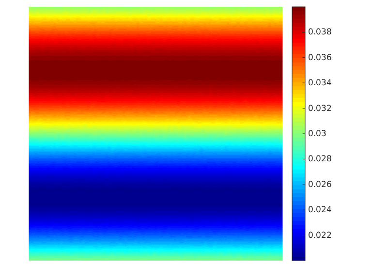
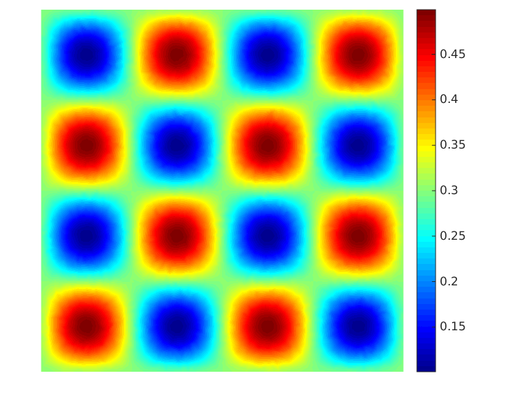
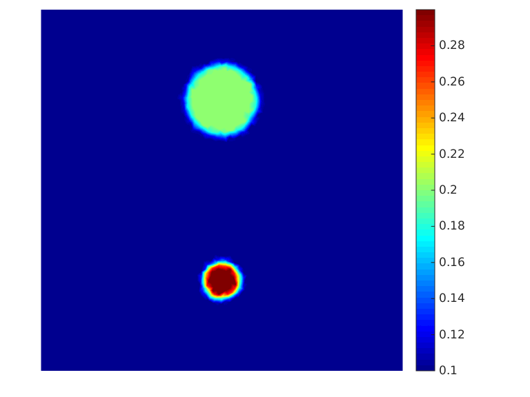
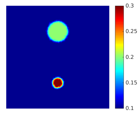
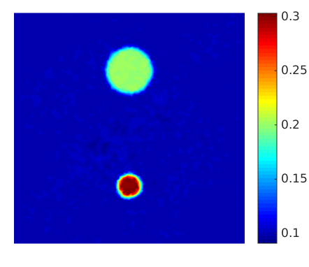
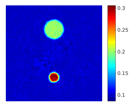
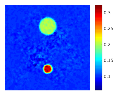
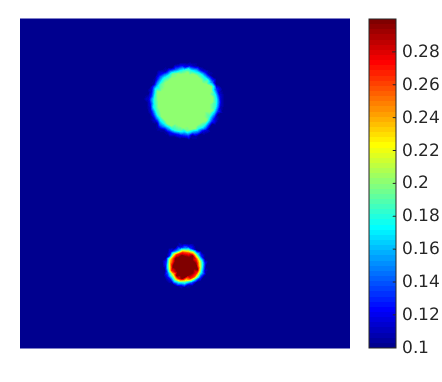
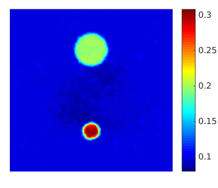
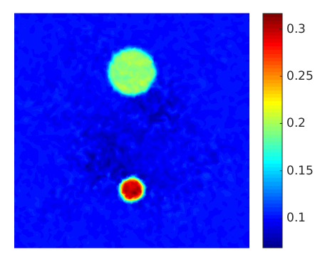
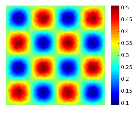
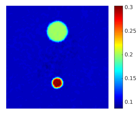
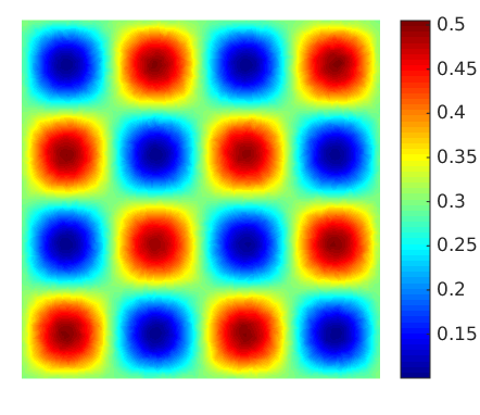
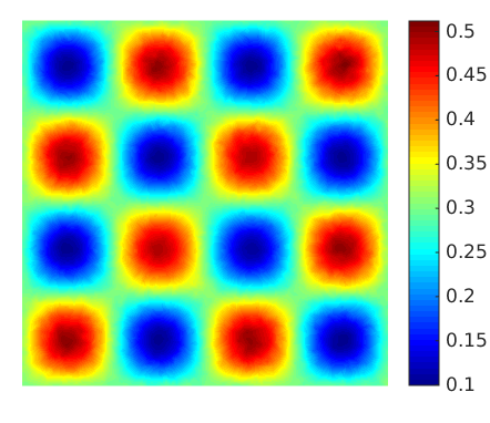
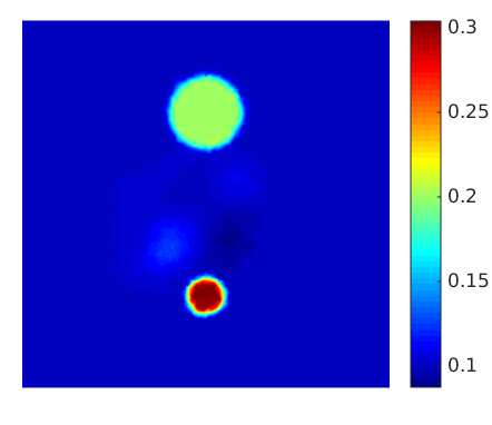
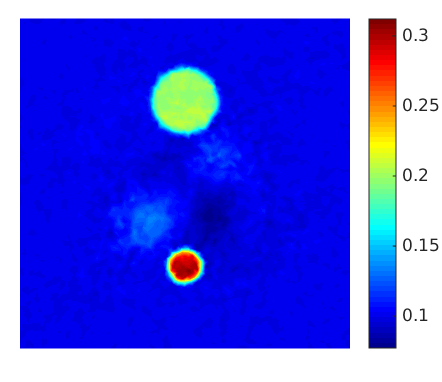
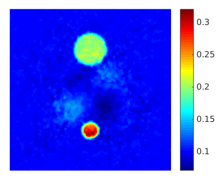
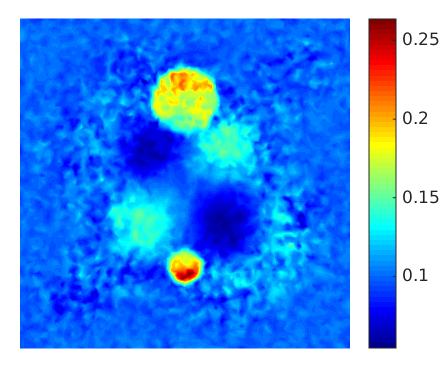
We start with a set of numerical experiments on the reconstruction of the two-photon absorption coefficient assuming that the single-photon absorption coefficient is known. We use data collected from four different sources , . We perform reconstructions using the Direct Algorithm. In Fig. 2 we show the reconstruction results from noisy synthetic data with noise levels , , , and . The true coefficients used to generate the data are shown in Fig. 1.
To measure the quality of the reconstruction, we use the relative error. This error is defined as the ratio between (i) the norm of the difference between the reconstructed coefficient and the true coefficient and (ii) the norm of the true coefficient, expressed in percentage. The relative errors in the reconstructions of in Fig 2 are , ,, and for , , and respectively.

Experiment II.
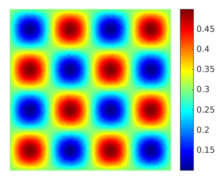
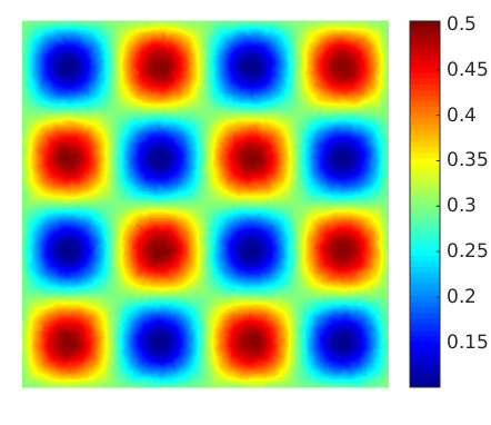
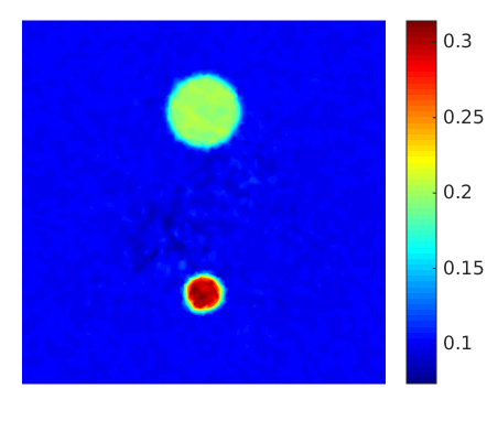
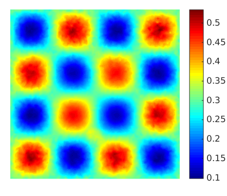
One of the main limitations on the Direct Algorithm is that it requires the use of illumination sources that are positive everywhere on the boundary. This is difficult to implement in practical applications. The Least-Square Algorithm, however, does not have such requirement on the optical sources (but it is computationally more expensive). Here we repeat the simulations in Experiment I with the Least-Square Algorithm. The reconstruction results are shown in Fig 3. We observe that, with the same (not exactly the same since the realizations of the noise are different) data sets, the reconstructions from the two different algorithms are of very similar quality. The relative errors for the reconstructions in Fig 3 are , ,, and respectively for the four cases.


Experiment III.
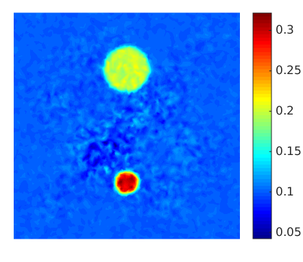
In the third set of numerical experiments, we study the simultaneous reconstructions of the single-photon and two-photon absorption coefficients, and . We again use data collected from four different sources. In Fig. 4, we show the reconstructions from data containing different noise levels using the Direct Algorithm. The relative error in the reconstructions of are , ,, and respectively for data with noise levels , , and .

Experiment IV.
We now repeat the simulations in Experiment III with the Least-Square Algorithm. The results are shown in Fig. 5. The relative errors in the reconstructions are now , ,, respectively for data with noise levels , , , and . The quality of the reconstructions is slightly lower than, but still comparable to, that in the reconstructions in Experiment III.
We observe from the above simulation results that, in general, the quality of the reconstructions is very high. When we have the illumination sources that satisfy the positivity requirement on the whole boundary of the domain, the Direct Algorithm provides an efficient and robust reconstruction method. The Least-Square Algorithm is less efficient but is as robust in terms of the quality of the reconstructions. The reconstructions with the Least-Square Algorithm are done for a fixed regularization parameter that we selected by a couple of trial-error test. It is by no means the optimal regularization parameter that can be selected through more sophisticated algorithms [22]. However, this is an issue that we think is not important at the current stage of this project. Therefore, we did not pursue further in this direction.
We also observe that the performances of the reconstructions of and are different in both the direct and the least-square methods: the reconstructions of is visually better than those of in general. This phenomenon is not manifested in our current stability results. Further analysis, for instance to refine the stability results in Section 3, are needed to fully understand this difference in numerical stability.
6 Conclusion and further remarks
We studied in this paper inverse problems in quantitative photoacoustic tomography with two-photon absorption. We derived uniqueness and stability results in the reconstruction of single-photon and two-photon absorption coefficients, and proposed explicit reconstruction methods in this case with well-selected illumination sources. We also studied the inverse problem of reconstructing the diffusion coefficient in addition to the absorption coefficients and obtained partial results on the uniqueness and stability of the reconstructions for the linearized problem. We presented some numerical studies based on the explicit reconstruction procedures as well as numerical optimization techniques to demonstrate the type of quality that can be achieved in reasonably controlled environments (where noise strength in the data is moderate).
Our focus in this paper is to study the mathematical properties of the inverse problems. There are many issues that have to be address in the future. Mathematically, it would be nice to generalize the uniqueness and stability results in Section 4, on multiple coefficient reconstructions in linearized settings, to the fully nonlinear problem. Computationally, detailed numerical analysis, in three-dimensional setting, need to be performed to quantify the errors in the reconstructions in practically relevant scenarios. It is especially important to perform reconstructions starting from acoustic data directly, following for instance the one-step reconstruction strategy developed in [19], to see how sensitive the reconstruction of the two-photon absorption coefficient is with respect to noise in the acoustic data. On the modeling side, it is very interesting to see if the current study can be generalized to radiative transport type models for photon propagation.
Acknowledgments
We would like to the anonymous referees for their useful comments that help us improve the quality of the paper. This work is partially supported by the National Science Foundation through grants DMS-1321018 and DMS-1620473.
Appendix A: Terminologies in overdetermined elliptic systems
We recall here, very briefly, some terminologies and notations related to overdetermined linear elliptic systems, following the presentation in [7, 54]. Let be three positive integers such that . we consider the following system of differential equations for variables with boundary conditions:
| (53) | |||||
| (54) |
Here is a matrix differential operator whose element, denoted by (, ), is a polynomial in for any . is a matrix differential operator whose element, denoted by (, ), is a polynomial in for any .
We associate an integer () to row of and an integer to column () of .
Definition 6.1.
We call the integers and the Douglis-Nirenberg numbers associated to if: (a) , ; (b) when , the order of is not greater than ; and (c) when , .
Definition 6.2.
The principal part of , denoted by , is defined as the part of such that the degree of is exactly .
We say that is elliptic, in the sense of Douglis-Nirenberg, if the matrix is of rank for all ( being the unit sphere in ) and all .
Let be the order of and define
| (55) |
Definition 6.3.
The principal part of , denoted by , is defined as the part of such that the order of is exactly .
Let be the principal part of . Fix , and let be the inward unit normal vector at . Let be a vector such that and . We consider on the half line the system of ordinary equations
| (56) | |||||
| (57) |
Definition 6.4.
It is well-established that [7, 47, 54] when satisfies the Lopatinskii criterion, the system (53)-(54) can be solved up to possibly a finite dimensional subspace. Moreover, a general a priori stability estimate can be established for the system. Define the function space
for some . Then it can be shown that, if ,
| (58) |
provided that all the quantities involved are regular enough. The last term in the estimate can be dropped when uniqueness of the solution can be proven. More details of this theory can be found in [7] and references therein.
Appendix B: CGO solutions to equation (1)
This appendix is devoted to the construction of complex geometric optics (CGO) solutions [49, 51] to our model equation (1). We restrict the construction to the three-dimensional setting (). We start by revisiting CGO solutions to the classical diffusion problem that was first developed in [49]:
| (59) |
with the assumption that and . Let be a solution to this equation, then the Liouville transform defined in (26) shows that solves
| (60) |
The following result is well-known.
Theorem 6.5 ([6, 49, 51]).
Let and . For any such that and sufficiently large, there is a function such that the solution to (60), with the boundary condition , takes the form
| (61) |
with satisfying the estimate
| (62) |
The function is called a complex geometric optics solution to (60) and
| (63) |
is a complex geometric optics solution to (59). With the regularity assumption on and (62), it is easy to verify that
| (64) |
We now show, using the Newton-Kantorovich method [41], that we can construct a CGO solution to our semilinear diffusion model that is very close, in , to for some .
Theorem 6.6.
Let , and . Let be such that and sufficiently large. Assume further that and satisfy
| (65) |
for some . Then, there exists a function such that the solution to (1) takes the form
| (66) |
with such that
| (67) |
for some constant and some .
Proof.
We first observe that the assumption in (65) allows us to bound the CGO solution and its gradient as
| (68) |
| (69) |
Let be the differential operator defined in (1). We verify that, with the assumptions on the coefficients involved, , the linearization of at , , admits a bounded inverse as a linear map from to .
We observe from the construction that is away from . Therefore, there exists a constant such that the ball (in the metric) contains functions that are away from . Let , and be given, we check that
| (70) |
This leads to
| (71) |
We can also bound as follows. We first verify that
| (72) |
We then perform the expansion, using the fact that (),
This gives us the bound
| (73) |
We can then combine (72) with (73) and use Sobolev embedding, for instance [27, Corollary 7.11], to conclude that
| (74) |
Let us remark that the assumption (65) on and is feasible. Let be a basis of . Since is bounded, we can place in a box in the first octant of the system. Let us take for some . We check that we can have for some constant and . If we further take to be proportional to , we can have (65); see Section 4 for the choices of different in our analysis.
References
- [1] G. Alessandrini, M. Di Cristo, E. Francini, and S. Vessella, Stability for quantitative photo acoustic tomography with well-chosen illuminations, Annali di Matematica, 196 (2017), pp. 395–406.
- [2] A. Ambrosetti and A. Malchiodi, Nonlinear Analysis and Semilinear Elliptic Problems, Cambridge University Press, Cambridge, 2007.
- [3] H. Ammari, E. Bossy, V. Jugnon, and H. Kang, Mathematical modelling in photo-acoustic imaging of small absorbers, SIAM Rev., 52 (2010), pp. 677–695.
- [4] H. Ammari, E. Bretin, V. Jugnon, and A. Wahab, Photo-acoustic imaging for attenuating acoustic media, in Mathematical Modeling in Biomedical Imaging II, H. Ammari, ed., vol. 2035 of Lecture Notes in Mathematics, Springer-Verlag, 2012, pp. 53–80.
- [5] M. Badiale and E. Serra, Semilinear Elliptic Equations for Beginners, Springer, London, 2011.
- [6] G. Bal, Introduction to Inverse Problems. Department of Applied Physics and Applied Mathematics, Columbia University, 2012.
- [7] , Hybrid inverse problems and redundant systems of partial differential equations, in Inverse Problems and Applications, P. Stefanov, A. Vasy, and M. Zworski, eds., vol. 615 of Contemporary Mathematics, American Mathematical Society, 2013, pp. 15–48.
- [8] G. Bal and K. Ren, Multi-source quantitative PAT in diffusive regime, Inverse Problems, 27 (2011). 075003.
- [9] , Non-uniqueness result for a hybrid inverse problem, in Tomography and Inverse Transport Theory, G. Bal, D. Finch, P. Kuchment, J. Schotland, P. Stefanov, and G. Uhlmann, eds., vol. 559 of Contemporary Mathematics, Amer. Math. Soc., Providence, RI, 2011, pp. 29–38.
- [10] , On multi-spectral quantitative photoacoustic tomography in diffusive regime, Inverse Problems, 28 (2012). 025010.
- [11] G. Bal and G. Uhlmann, Inverse diffusion theory of photoacoustics, Inverse Problems, 26 (2010). 085010.
- [12] P. Beard, Biomedical photoacoustic imaging, Interface Focus, 1 (2011), pp. 602–631.
- [13] F. Bouchut and G. Crippa, Uniqueness, renormalization and smooth approximations for linear transport equations, SIAM J. Math. Anal., 38 (2006), pp. 1316–1328.
- [14] P. Burgholzer, G. J. Matt, M. Haltmeier, and G. Paltauf, Exact and approximative imaging methods for photoacoustic tomography using an arbitrary detection surface, Phys. Rev. E, 75 (2007). 046706.
- [15] F. Colombini, G. Crippa, and J. Rauch, A note on two-dimensional transport with bounded divergence, Comm. Partial Differential Equations, 31 (2006), pp. 1109–1115.
- [16] B. T. Cox, S. R. Arridge, and P. C. Beard, Photoacoustic tomography with a limited-aperture planar sensor and a reverberant cavity, Inverse Problems, 23 (2007), pp. S95–S112.
- [17] B. T. Cox, S. R. Arridge, K. P. Köstli, and P. C. Beard, Two-dimensional quantitative photoacoustic image reconstruction of absorption distributions in scattering media by use of a simple iterative method, Applied Optics, 45 (2006), pp. 1866–1875.
- [18] B. T. Cox, J. G. Laufer, and P. C. Beard, The challenges for quantitative photoacoustic imaging, Proc. of SPIE, 7177 (2009). 717713.
- [19] T. Ding, K. Ren, and S. Vallelian, A one-step reconstruction algorithm for quantitative photoacoustic imaging, Inverse Problems, 31 (2015), p. 095005.
- [20] R. J. DiPerna and P.-L. Lions, On the Cauchy problem for Boltzmann equations: global existence and weak stability, Ann. Math., 130 (1989), pp. 321–366.
- [21] A. Douglis and L. Nirenberg, Interior estimates for elliptic system of partial differential equations, Comm. Pure Appl. Math., 8 (1955), pp. 503–508.
- [22] H. W. Engl, M. Hanke, and A. Neubauer, Regularization of Inverse Problems, Kluwer Academic Publishers, Dordrecht, The Netherlands, 1996.
- [23] L. C. Evans, Partial Differential Equations, American Mathematical Society, Providence, RI, 2010.
- [24] D. Finch, M. Haltmeier, and Rakesh, Inversion of spherical means and the wave equation in even dimensions, SIAM J. Appl. Math., 68 (2007), pp. 392–412.
- [25] A. R. Fisher, A. J. Schissler, and J. C. Schotland, Photoacoustic effect for multiply scattered light, Phys. Rev. E, 76 (2007). 036604.
- [26] H. Gao, S. Osher, and H. Zhao, Quantitative photoacoustic tomography, in Mathematical Modeling in Biomedical Imaging II: Optical, Ultrasound, and Opto-Acoustic Tomographies, H. Ammari, ed., vol. 2035 of Lecture Notes in Mathematics, Springer, 2012, pp. 131–158.
- [27] D. Gilbarg and N. S. Trudinger, Elliptic Partial Differential Equations of Second Order, Springer-Verlag, Berlin, 2000.
- [28] M. Haltmeier, T. Schuster, and O. Scherzer, Filtered backprojection for thermoacoustic computed tomography in spherical geometry, Math. Methods Appl. Sci., 28 (2005), pp. 1919–1937.
- [29] Q. Han and F. Lin, Elliptic Partial Differential Equations, American Mathematical Society, Providence, 1997.
- [30] M. Hauray, On two-dimensional Hamiltonian transport equations with coefficients, Ann. IHP. Anal. Non Lin., 20 (2003), pp. 625–644.
- [31] Y. Hristova, Time reversal in thermoacoustic tomography - an error estimate, Inverse Problems, 25 (2009). 055008.
- [32] A. Kirsch and O. Scherzer, Simultaneous reconstructions of absorption density and wave speed with photoacoustic measurements, SIAM J. Appl. Math., 72 (2013), pp. 1508–1523.
- [33] P. Kuchment and L. Kunyansky, Mathematics of thermoacoustic tomography, Euro. J. Appl. Math., 19 (2008), pp. 191–224.
- [34] P. Kuchment and D. Steinhauer, Stabilizing inverse problems by internal data, Inverse Problems, 28 (2012).
- [35] Y.-H. Lai, S.-Y. Lee, C.-F. Chang, Y.-H. Cheng, and C.-K. Sun, Nonlinear photoacoustic microscopy via a loss modulation technique: from detection to imaging, Optics Express, 22 (2014), pp. 525–536.
- [36] G. Langer, K.-D. Bouchal, H. Grün, P. Burgholzer, and T. Berer, Two-photon absorption-induced photoacoustic imaging of Rhodamine B dyed polyethylene spheres using a femtosecond laser, Optics Express, 21 (2013), pp. 22410–22422.
- [37] J. Laufer, B. T. Cox, E. Zhang, and P. Beard, Quantitative determination of chromophore concentrations from 2d photoacoustic images using a nonlinear model-based inversion scheme, Applied Optics, 49 (2010), pp. 1219–1233.
- [38] C. Li and L. Wang, Photoacoustic tomography and sensing in biomedicine, Phys. Med. Biol., 54 (2009), pp. R59–R97.
- [39] A. V. Mamonov and K. Ren, Quantitative photoacoustic imaging in radiative transport regime, Comm. Math. Sci., 12 (2014), pp. 201–234.
- [40] L. V. Nguyen, A family of inversion formulas in thermoacoustic tomography, Inverse Probl. Imaging, 3 (2009), pp. 649–675.
- [41] J. M. Ortega, The Newton-Kantorovich theorem, Amer. Math. Monthly, 75 (1968), pp. 658–666.
- [42] A. Pulkkinen, B. T. Cox, S. R. Arridge, J. P. Kaipio, and T. Tarvainen, A Bayesian approach to spectral quantitative photoacoustic tomography, Inverse Problems, 30 (2014). 065012.
- [43] K. Ren, G. Bal, and A. H. Hielscher, Frequency domain optical tomography based on the equation of radiative transfer, SIAM J. Sci. Comput., 28 (2006), pp. 1463–1489.
- [44] K. Ren, H. Gao, and H. Zhao, A hybrid reconstruction method for quantitative photoacoustic imaging, SIAM J. Imag. Sci., 6 (2013), pp. 32–55.
- [45] K. Ren, R. Zhang, and Y. Zhong, Inverse transport problems in quantitative PAT for molecular imaging, Inverse Problems, 31 (2015). 125012.
- [46] T. Saratoon, T. Tarvainen, B. T. Cox, and S. R. Arridge, A gradient-based method for quantitative photoacoustic tomography using the radiative transfer equation, Inverse Problems, 29 (2013). 075006.
- [47] V. A. Solonnikov, Overdetermined elliptic boundary-value problems, J. Sov. Math., 1 (1973), pp. 477–512.
- [48] P. Stefanov and G. Uhlmann, Thermoacoustic tomography with variable sound speed, Inverse Problems, 25 (2009). 075011.
- [49] J. Sylvester and G. Uhlmann, Global uniqueness theorem for an inverse boundary value problem, Ann. Math., 125 (1987), pp. 153–169.
- [50] G. J. Tserevelakis, D. Soliman, M. Omar, and V. Ntziachristos, Hybrid multiphoton and optoacoustic microscope, Opt. Lett., 39 (2014), pp. 1819–1822.
- [51] G. Uhlmann, Electrical impedance tomography and Calderon’s problem, Inverse Problems, 25 (2009). 123011.
- [52] B. E. Urban, J. Yi, V. Yakovlev, and H. F. Zhang, Investigating femtosecond-laser-induced two-photon photoacoustic generation, J. Biomed. Opt., 19 (2014). 085001.
- [53] L. V. Wang, Tutorial on photoacoustic microscopy and computed tomography, IEEE J. Sel. Topics Quantum Electron., 14 (2008), pp. 171–179.
- [54] T. Widlak and O. Scherzer, Stability in the linearized problem of quantitative elastography, Inverse Problems, 31 (2015). 035005.
- [55] P. W. Winter, A. G. York, D. D. Nogare, M. Ingaramo, R. Christensen, A. Chitnis, G. H. Patterson, and H. Shroff, Two-photon instant structured illumination microscopy improves the depth penetration of super-resolution imaging in thick scattering samples, Optica, 1 (2014), pp. 181–191.
- [56] Y. Yamaoka, M. Nambu, and T. Takamatsu, Frequency-selective multiphoton-excitation-induced photoacoustic microscopy (MEPAM) to visualize the cross sections of dense objects, in Photons Plus Ultrasound: Imaging and Sensing, A. A. Oraevsky and L. V. Wang, eds., SPIE, 2010. 75642O.
- [57] , Fine depth resolution of two-photon absorption-induced photoacoustic microscopy using low-frequency bandpass filtering, Optics Express, 19 (2011), pp. 13365–13377.
- [58] Y. Yamaoka and T. Takamatsu, Enhancement of multiphoton excitation-induced photoacoustic signals by using gold nanoparticles surrounded by fluorescent dyes, in Photons Plus Ultrasound: Imaging and Sensing, A. A. Oraevsky and L. V. Wang, eds., SPIE, 2009. 71772A.
- [59] C. S. Yelleswarapu and S. R. Kothapalli, Nonlinear photoacoustics for measuring the nonlinear optical absorption coefficient, Optics Express, 18 (2010), pp. 9020–9025.
- [60] R. J. Zemp, Quantitative photoacoustic tomography with multiple optical sources, Applied Optics, 49 (2010), pp. 3566–3572.