Powheg–Pythia matching scheme effects in
NLO simulation of dijet events

Abstract

One of the most important developments in Monte Carlo simulation of collider events for the LHC has been the arrival of schemes and codes for matching of parton showers to matrix elements calculated at next-to-leading order in the QCD coupling. The Powheg scheme, and particularly its implementation in the Powheg-Box code, has attracted most attention due to ease of use and effective portability between parton shower algorithms.

But formal accuracy to NLO does not guarantee predictivity, and the beyond-fixed-order corrections associated with the shower may be large. Further, there are open questions over which is the “best” variant of the Powheg matching procedure to use, and how to evaluate systematic uncertainties due to the degrees of freedom in the scheme.

In this paper we empirically explore the scheme variations allowed in Pythia 8 matching to Powheg-Box dijet events, demonstrating the effects of both discrete and continuous freedoms in emission vetoing details for both tuning to data and for estimation of systematic uncertainties from the matching and parton shower aspects of the Powheg-Box +Pythia 8 generator combination.

MCnet-16-34

Introduction

One of the most important recent developments in Monte Carlo simulation of collider events has been the arrival of schemes and codes for consistent parton-shower dressing of partonic hard process matrix elements calculated at next-to-leading order in the QCD coupling.

It is now possible to simulate fully exclusive event generation in which the parton shower (PS) is smoothly matched to matrix element (ME) calculations significantly improved over the leading-order Born level, and the modelling further improved by non-perturbative modelling aspects such as hadronization and multiple partonic interactions (MPI). Tools providing these improvements include both “multi-leg LO”, exemplified by the Alpgen [1], MadGraph [2], and Sherpa 1 [3] codes; the “single-emission NLO” codes such as Powheg-Box [4] and (a)MC@NLO [5, 6]; and the latest generation in which both modes are combined into shower-matched multi-leg NLO: Sherpa 2 and MadGraph5-aMC@NLO [7].

While the technical and bookkeeping details in these algorithms for combination of different-multiplicity matrix elements and parton showers are formidable, and their availability has revolutionised the approaches taken to physics analysis during the LHC era, there remain constant questions about how to evaluate the uncertainties in the methods. Which generator configuration choices are absolute and unambiguous, and which have degrees of freedom which can be exploited either for more accurate data-description (of primary interest to new physics search analyses) or to construct a theory systematic uncertainty in comparisons of QCD theory to data (the “Standard Model analysis” attitude). Despite the confidence-inspiring “NLO” label on many modern showering generators, there are in practice many freedoms in matching matrix elements to shower generators.

The Powheg scheme, in particular its implementation in the Powheg-Box code [4], has attracted most attention due to its ease of use and formal lack of dependence on the details of the parton shower used. But formal accuracy to NLO does not guarantee predictivity, and the beyond-fixed-order corrections induced by the shower procedure may be large. Further, questions remain over which is the “best” variant of the Powheg matching procedure to use, and how to evaluate systematic uncertainties due to the degrees of freedom in the scheme. Since the extra parton production in Powheg real-emission events suppresses the phase space for parton shower emission, use of such ME–PS matching can lead to underestimation of total systematic uncertainties unless the matching itself is considered as a potential source of uncertainty in addition to the Powheg matrix element scales and the (suppressed) Pythia parton showers.

In this paper we empirically explore the scheme variations allowed in Pythia 8 [8] matching to Powheg-Box dijet [9] events, demonstrating the potentially disastrous effects of “reasonable” matching choices and the remaining tuning freedom for optimal data description.

1 Powheg matching variations in Pythia 8

The original and simplest approach to showering Powheg events is to start parton shower evolution at the characteristic scale declared by the input event. Since the Powheg formalism works via a shower-like Sudakov form factor, and both Powheg-Box and the Pythia parton showers produce emissions ordered in relative transverse momentum, this approach seems intuitively correct. But in fact the definition of “relative transverse momentum” is not quite the same between the two codes and hence this approach may double-count some phase-space regions, and fail to cover others entirely.

Pythia’s answer to this is to provide machinery for “shower vetoing”, i.e. to propose parton shower emissions over all permitted phase space (including above the input event scale, up to the beam energy threshold) according to Pythia’s emission-hardness definition, but to veto any proposal whose Powheg definition of “hardness” is above the threshold declared by or calculated from the input event. This machinery is most easily accessed via the main31 Pythia 8 example program.

But there are still ambiguities, since the Powheg method itself does not prescribe exactly what form of vetoing variable should be used. Pythia 8 makes three discrete choices available for calculation of the Powheg-hardness scales to be used in the shower-emission vetoing. These are controlled via the configuration flags pTdef, pTemt, and pThard, which respectively determine the variable(s) to be used to define “hardness” in the Powheg shower-veto procedure, the partons to be used in computing their values, and the cut value(s) to be used in applying that hardness veto to the calculated hardness variables.

The available variations of these scale calculations range from comparison of the matched emission against only a limited subset of event particles at one extreme, to comparison with all available particles at the other. This typically produces a spectrum of scale values to characterise a shower emission, from maximal scales at one end to minimal scales at the other, with a spectrum of in-between values from hybrid approaches. The effect on shower emission vetoing depends on the combination of the scale calculated for each proposed shower emission and the scale threshold determined from the input event.

Testing all options of all three scales simultaneously would produce 50 or so predictions to be compared and disambiguated: not a pleasant task for either us or the reader! So we instead take a divide-and-conquer approach, first focusing on the pTemt scale alone since it has been observed to produce large effects in many observables. We then proceed via a reduced set of preferred pTemt schemes, on which to study further variations.

In all the following comparisons and discussion the combination of scale calculation schemes are represented by an integer tuple $HED=(\text{{pThard}},\text{{pTemt}},\text{{pTdef}})$. The default Pythia 8 Powheg matching configuration is $HED=201$ in this notation.

1.1 Methodology

All the plots shown in this study were computed using ATLAS and CMS jet analyses encoded in the Rivet 2.4 [10] analysis system. All such available analyses at the time of the study used $pp$ events with $\sqrt{s}=7~{}\text{T$\text{e}\mspace{-0.8mu}\text{V}$}$. 10 million input events for the analyses were generated in LHE format [11] by Powheg-Box v2 r3144 and processed in parallel through Pythia  8.212 using the main31 example program, default tune & PDF, and HepMC event record output [12].

The full set of Rivet analyses used is listed in Table 1, giving a comprehensive view of the effects of matching scheme variations across the public LHC measurements of hadronic jet production. For obvious reasons of space and exposition, in this paper we only show a small representative subset of these plots, but all 920 (!) have been considered in the discussion of observed effects.

Rivet analysis name	Description & citation
ATLAS analyses
ATLAS_2014_I1326641	3-jet cross-section [13]
ATLAS_2014_I1325553	Inclusive jet cross-section [14]
ATLAS_2014_I1307243	Jet vetoes and azimuthal decorrelations in dijet events [15]
ATLAS_2014_I1268975	High-mass dijet cross-section [16]
ATLAS_2012_I1183818	Pseudorapidity dependence of total transverse energy [17]
ATLAS_2012_I1119557	Jet shapes and jet masses [18]
ATLAS_2012_I1082936	Inclusive jet and dijet cross-sections [19]
ATLAS_2011_S9128077	Multi-jet cross-sections [20]
ATLAS_2011_S9126244	Dijet production with central jet veto [21]
ATLAS_2011_S8971293	Dijet azimuthal decorrelations [22]
ATLAS_2011_S8924791	Jet shapes [23]
ATLAS_2010_S8817804	Inclusive jet cross-section + dijet mass and $\chi$ spectra [24]
CMS analyses
CMS_2014_I1298810	Ratios of jet $p_{\mathrm{T}}$ spectra [25]
CMS_2013_I1224539_DIJET	Jet mass measurement in dijet events [26]
CMS_2013_I1208923	Jet $p_{\mathrm{T}}$ and dijet mass [27]
CMS_2012_I1184941	Inclusive dijet production as a function of $\xi$ [28]
CMS_2012_I1090423	Dijet angular distributions [29]
CMS_2012_I1087342	Forward and forward + central jets [30]
CMS_2011_S9215166	Forward energy flow in dijet events [31]
CMS_2011_S9088458	Ratio of 3-jet over 2-jet cross-sections [32]
CMS_2011_S9086218	Inclusive jet cross-section [33]
CMS_2011_S8968497	Dijet angular distributions [34]
CMS_2011_S8950903	Dijet azimuthal decorrelations [35]

Table 1: List of Rivet analyses used for the jet observables studied in this paper. All analyses were performed on $pp$ data at $\sqrt{s}=7~{}\text{T$\text{e}\mspace{-0.8mu}\text{V}$}$.

1.2 Variation of pTemt

In Figure 1 we show the effects of varying the pTemt scale calculation; for clarity only the combinations with the main31 default $\text{{pTdef}}=2$ and $\text{{pThard}}=1$ settings are shown, since the pTemt effects by far dwarf those from the two remaining degrees of freedom.

(a)

(b)

Figure 1: Observables showing the effect of pTemt variation. The 3-digit tuple used in the plot legends represents the Pythia 8 $HED$ flag combination as described in the text.

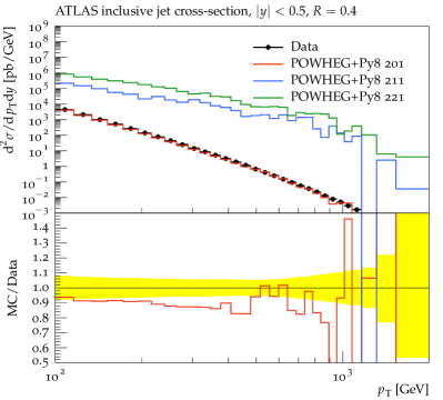
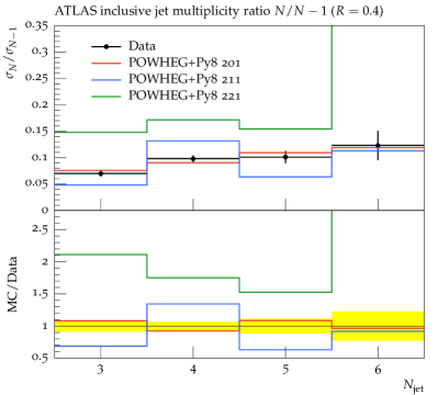
The values 0–2 of pTemt have the following meanings, relating to the “hardness” of a proposed shower emission, to be compared to the vetoing hardness cut specified by the Powheg method and the hard-process event kinematics:

0:

hardness calculated for the emitted parton only, with respect to the radiating parton only, and recoil effects are neglected;

1:

hardness calculated for the emitted parton, computed with respect to all partons (initial and final), and the minimum such value is used;

2:

hardness calculated for all final-state partons, computed with respect to all other partons, and the minimum value used.

Scheme 0 is the hardness definition used by the Powheg-Box itself, in the hard process events supplied to Pythia, and is hence a priori expected to give the best matching. Since the other schemes consider hardness relative to partons other than the emitter and take the smallest, they will in general produce lower hardness scales for proposed shower emissions and hence fewer such emissions will be vetoed.

The left-hand plot shows the $p_{\mathrm{T}}$ distribution of inclusive jets in the most central rapidity bin as measured by ATLAS in 7 TeV $pp$ collisions [14], where the effect of using a non-default pTemt scheme is a cross-section overestimation by factors of 50–300. The Powheg matching details can hence be exceedingly important, potentially more-so than standard systematic variations on matrix element scales and PDFs. The right-hand plot shows the effect of pTemt on jet multiplicity ratios: a much smaller effect, but still a source of significant mismodelling.

It is clear that these are huge effects, utterly incompatible with the data. The only viable combinations of $HED$ parameters have $\text{{pTemt}}=0$, i.e. the largest of the possible values for the Powheg hardness scales since $\text{{pTemt}}=1$ or 2 can only be less than or equal to the $\text{{pTemt}}=0$ value. The lower hardness values computed for Pythia shower emissions would result in less emission-vetoing and hence harder distribution tails.

In fact, details like jet vetos, jet shapes, and $E_{\mathrm{T}}$ flow can be moderately well described by the configurations which produce such large jet mass and $p_{\mathrm{T}}$ tails. This makes sense for single-jet quantities which are at first-order independent of overall event activity, but is less obvious for the global event variables. It is clear, though, that from the available options the $\text{{pTemt}}=0$ configuration is the only viable choice for dijet simulation – while noting that it still displays a systematic data/MC discrepancy of up to 20%.

The extent to which these different scale calculation details can affect observables, independent of the choice of pTdef and pThard schemes, is potentially disturbing. The default $\text{{pTemt}}=0$ mode gives by far the closest agreement with data and is the definition most closely related to the NLO subtraction used in Powheg, but since there is no unambiguously correct calculation scheme there must be residual uncertainty over how large the effects of much more subtle variations in scale calculation could be. Given the obvious sensitivity of observables to this matching scheme detail, it will be interesting to explore whether minor refinements to the Pythia scale calculation can produce more reasonable variations, particularly one which might correct for the systematic undershooting of multi-jet mass measurements.

1.3 Variation of pThard and pTdef

(a)

(b)

(c)

(d)

Figure 2: Observables showing the effects of pThard and pTdef variations, with $\text{{pTemt}}=0$. The 3-digit tuple used in the plot legends represents the Pythia 8 $HED$ flag combination as described in the text.

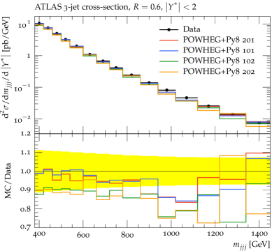
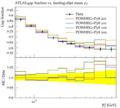
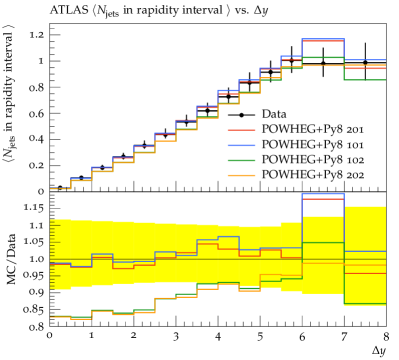
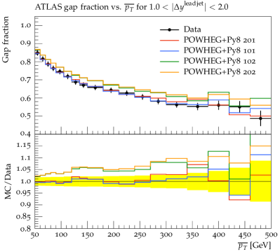
Having established that only the $\text{{pTemt}}=0$ configuration is viable, we now fix its value and explore four combinations of the other two matching flags, $\text{{pThard}}\in\{1,2\}$ and $\text{{pTdef}}\in\{1,2\}$; explicitly, the $HED$ tuples 201 (the Pythia 8 main31 example program setting), 101, 202, and 102. The pThard flag distinguishes between two methods for recalculation of the Powheg veto scale (as opposed to using the SCALUP value specified in the LHE file): a value of 1 considers the $p_{\mathrm{T}}$ of the Powheg emitted parton relative to all other partons, while a value of 2 uses the minimal $p_{\mathrm{T}}$ of all final state partons relative to all other partons. The pTdef flag switches between using the Powheg-Box or Pythia 8 definitions of “$p_{\mathrm{T}}$” in the veto scale calculation.

These variations are shown in Figures 2 to 4. The most distinctive feature of these histograms shown in these figures is that there are two consistent groups of MC curves in all cases: the 201 & 101 combinations together, and the 102 & 202 combinations together. It is hence clear that the pTdef mode (the 3rd component of the $HED$ tuple) has a stronger effect than pThard on these observables – the question is whether there is a clear preference for either grouping, and then whether there is distinguishing power between the finer pThard splitting within the preferred group.

All the (ATLAS) plots in Figure 2 favour the $\text{{pTdef}}=1$ grouping (the Powheg-Box $p_{\mathrm{T}}$ definition), in particular in the dijet rapidity gap analysis where description of small rapidity gaps and gaps between high mean-$p_{\mathrm{T}}$ dijet systems is significantly better than the $\text{{pTdef}}=2$ option. The distinction is less significant – within the experimental error band – for modelling of the 3-jet mass spectrum and for larger rapidity gaps & less energetic dijet systems.

(a)

(b)

(c)

(d)

Figure 3: Observables showing the effect of pThard and pTdef variations. The 3-digit tuple used in the plot legends represents the Pythia 8 $HED$ flag combination as described in the text.

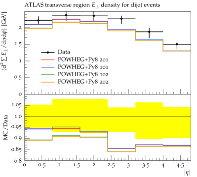
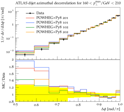
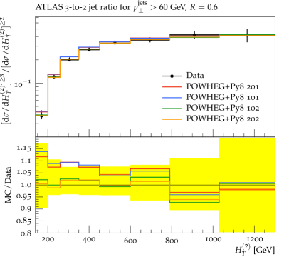
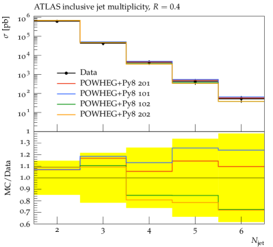
In Figure 3, again the picture is less clear: neither group of matching configurations describes transverse energy well as a function of $|\eta|$, and both models converge to the same (poor) description at high rapidity; the $\text{{pTdef}}=1$ configuration comes closer to the data at central rapidities, falling just within the experimental error band, but $\text{{pTdef}}=2$ more closely matches the flatter shape of the data. Interestingly, dijet azimuthal decorrelation data prefers the $\text{{pTdef}}=2$ “Pythia $p_{\mathrm{T}}$” treatment at the high-decorrelation (left-hand) end of the spectrum but this region of the observable is expected to be affected by multiple extra emissions and hence the performance of the single-emission Powheg scheme is not clearly relevant. The 3-to-2 jet ratio also somewhat prefers the Pythia $p_{\mathrm{T}}$ scheme, but both schemes lie within the experimental error bars, as they do for inclusive jet multiplicity modelling.

(a)

(b)

(c)

(d)

Figure 4: Observables showing the effect of pThard and pTdef variations. The 3-digit tuple used in the plot legends represents the Pythia 8 $HED$ flag combination as described in the text.

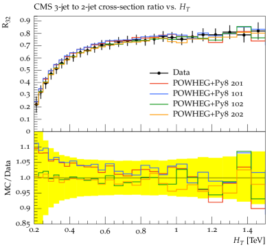
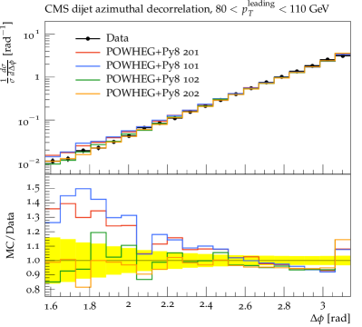
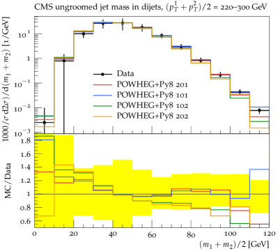
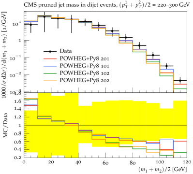
Finally, in Figure 4 we again see mixed results: CMS’ characterisations of the 3-to-2 jet ratio and dijet decorrelations also prefer $\text{{pTdef}}=2$, but the distribution of groomed jet masses exhibits a slight preference for the $\text{{pTdef}}=1$ Powheg-Box $p_{\mathrm{T}}$ scheme.

The consistent trend throughout these observables is that the Powheg-Box $p_{\mathrm{T}}$ definition produces more radiation, and hence larger $n$-jet masses, lower rapidity gap fractions, more jet decorrelation, and more 3-jet events. Some of these effects increase compatibility with data, while others prefer less radiation, as produced by using the Pythia $p_{\mathrm{T}}$ definition.

There is no clear “best” choice of pTdef scheme from the available observables, nor a consistent preference for either pThard scheme within the pTdef groupings. Pythia’s default $HED=201$ configuration is certainly viable based on this comparison, but a pTdef flip to the 202 configuration may be a preferable choice if jet multiplicities are more important than their relative kinematics (e.g. the multi-jet masses) for the application at hand.

We note that since the majority of these predictions fall within the experimental uncertainties and are hence viable competing models, but there are significant differences between them inside the experimental bands, pTdef variations may be a useful handle through which to estimate systematics uncertainties in Powheg +Pythia matched simulations.

2 $\alpha_{\mathrm{S}}$ dependence of matched observables

We conclude this short exploration of formal freedoms in Powheg +Pythia NLO matching by studying the effect of different forms of the running strong coupling $\alpha_{\mathrm{S}}(Q)$ in the parton shower. The Powheg matrix element necessarily uses an NLO $\alpha_{\mathrm{S}}$ running with fixed value $\alpha_{\mathrm{S}}(M_{Z})\sim 0.12$, for consistency with the NLO PDF used in the calculation. It hence seems natural that a parton shower matched to emissions using such an $\alpha_{\mathrm{S}}$ should itself use such a coupling.

But a counter-argument is that the parton shower, as an iterated approximation to the true QCD matrix elements for many-emission evolution, requires a large $\alpha_{\mathrm{S}}$ value to compensate for missing physics. This argument is formally expressed in the proposal for “CMW scaling” [36] of a “natural” $\alpha_{\mathrm{S}}$, in which its divergence scale $\Lambda_{\text{QCD}}$ is scaled up by an $N_{F}$-dependent factor between 1.5 and 1.7. Such a scaling increases the effective $\alpha_{\mathrm{S}}(M_{Z})$ of a “bare” NLO strong coupling. And empirically a fairly large $\alpha_{\mathrm{S}}$ is found to be preferred in MC tuning [37, 38, 39], in particular for description of final-state effects like jet shapes and masses. These large couplings can become as dramatic as $\alpha_{\mathrm{S}}(M_{Z})\sim 0.14$ without any ill effect on such observables. Whether one- or two-loop $\alpha_{\mathrm{S}}$ running is more appropriate in Powheg matching is also an open question with arguments possible in both directions.

Since several arguments can be made for using $\alpha_{\mathrm{S}}(M_{Z})$ values between 0.12 and 0.14 (respectively, consistency, CMW, and naked pragmatism), rather than explicitly perform CMW or similar scalings, we have explored 6 configurations with $\alpha_{\mathrm{S}}(M_{Z})\in\{0.12,0.13,0.14\}$ (”NLO-like”, ”LO-like” and ”enhanced LO”, respectively), and 1-loop and 2-loop running in each. Observables demonstrating these variations, each using 10M events with identical $\alpha_{\mathrm{S}}$ configurations in ISR and FSR showers, can be found in Figures 5 and 6.

(a)

(b)

(c)

(d)

Figure 5: Observables showing the effect of $\alpha_{\mathrm{S}}$ variation, in tandem for Pythia’s ISR and FSR parton showers. The legend indicates the values of $\alpha_{\mathrm{S}}(M_{Z})$ used to fix the running coupling, and whether a 1-loop or 2-loop $\beta$-function is being used.

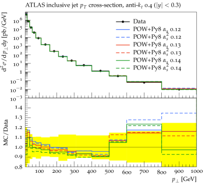
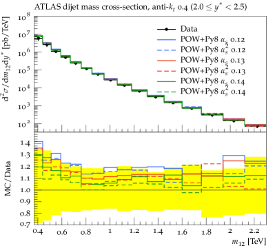
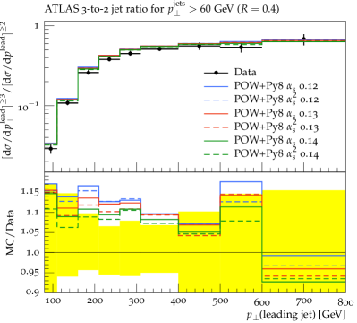
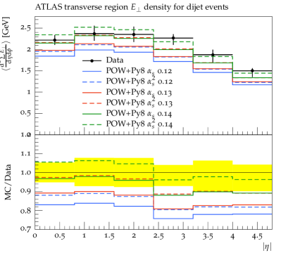
In Figure 5 all variations are grouped tightly within the experimental uncertainty band, but a clear trend of higher $\alpha_{\mathrm{S}}$ producing lower cross-sections is visible. A similar effect is visible in the dijet cross-section as a function of dijet mass, with all bins favouring a strong $\alpha_{\mathrm{S}}(M_{Z})=0.14$ with 2-loop running. Similar effects were seen for the equivalent CMS jet $p_{\mathrm{T}}$ spectra. The same strong $\alpha_{\mathrm{S}}$ settings are slightly but consistently preferred by the 3/2 jet ratio data, and the transverse energy flow also favours a large coupling, although not quite so extreme: either 1-loop $\alpha_{\mathrm{S}}(M_{Z})=0.14$ or 2-loop $\alpha_{\mathrm{S}}(M_{Z})=0.13$ work best. In all these observables, the steps of 0.1 in $\alpha_{\mathrm{S}}(M_{Z})$ have a similar magnitude of effect to the switches between 1-loop (“LO”) and 2-loop (“NLO”) running.

(a)

(b)

(c)

(d)

(e)

(f)

Figure 6: Observables showing the effect of $\alpha_{\mathrm{S}}$ variation. The legend indicates the values of $\alpha_{\mathrm{S}}(M_{Z})$ used to fix the running coupling, and whether a 1-loop or 2-loop $\beta$-function is being used. The left-hand column is for variation of the ISR shower $\alpha_{\mathrm{S}}$ only, and the right-hand column for variation of the FSR $\alpha_{\mathrm{S}}$ only. Due to Powheg matching, the ISR shower has essentially no effect, even on “ISR observables”.

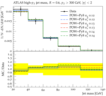
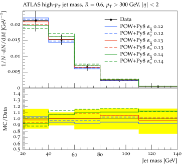
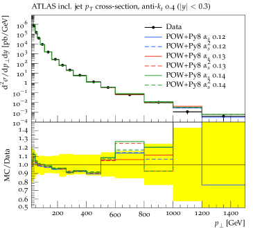
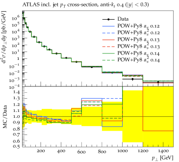
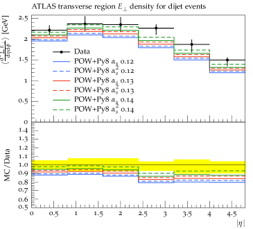
This is interesting: there is a fairly strong preference across much “ISR-influenced” data for a large shower coupling with $\alpha_{\mathrm{S}}(M_{Z})\sim 0.14$, even in Powheg-matched simulation. More generally, $\alpha_{\mathrm{S}}$ variations on this scale again provide useful coverage of experimental error bands and are hence a useful systematic handle on Powheg simulation.

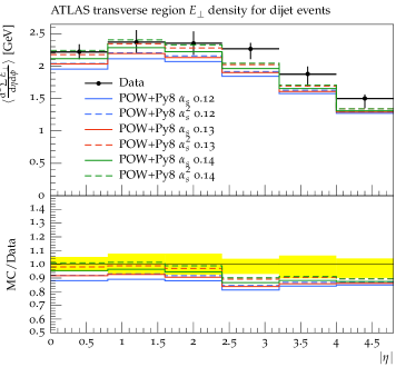
But FSR-dominated jet shapes and masses usually have a strong preference (if only due to the narrowness of jet shape experimental uncertainty bands) for a slightly smaller $\alpha_{\mathrm{S}}(M_{Z})\sim 0.13$. While matching might imply a need for consistency between ISR and FSR shower configurations, we are already operating in a regime beyond the formal accuracy of the method, and it is intriguing to see whether a hybrid setup with $\alpha_{\mathrm{S}}(M_{Z})\sim 0.14$ in the initial-state shower and $\alpha_{\mathrm{S}}(M_{Z})\sim 0.13$ in the final-state shower would give the best of both worlds across “ISR” and “FSR” observables. We do this by separately setting one shower $\alpha_{\mathrm{S}}(M_{Z})$ to the default 0.13 and varying the other, and vice versa, with results shown in Figure 6.

The results are illuminating: while as usual changes in the ISR shower have little effect on jet masses, they also have no effect on jet $p_{\mathrm{T}}$– a classic “ISR” observable. This pattern was repeated for all “ISR observables”, with virtually zero effect of the ISR shower coupling in all cases. The only variable to exhibit ISR shower sensitivity is the soft-QCD-dominated transverse energy flow, which is equally determined by ISR and FSR showering. While naïvely counter-intuitive, this makes perfect sense: the Powheg hard process is providing almost all the ISR effects, and leaving little phase space for the initial-state shower to produce effects on hard jet observables. These plots hence illustrate that the FSR shower configuration can have significant effects upon Powheg matching, and that there is a tension between the higher FSR $\alpha_{\mathrm{S}}$ desired to describe 3/2 jet ratios and multi-jet mass spectra, and the slightly lower values to describe intra-jet effects such as single-jet masses.

3 Summary

In this note we have explored several freedoms in Pythia 8’s machinery for matching parton showers to hard process partonic events generated by the Powheg-Box MC generator. These have included discrete options for defining and calculating the Powheg emission vetoing scale, and the continuous freedom to vary the strong coupling in Pythia’s parton showers.

All these freedoms are permitted within the fixed-order accuracy of the Powheg method, but it is clear that some will be better choices than others. We have hence considered the full set of 7 TeV $pp$ data analyses available from the ATLAS and CMS collaborations, via the Rivet analysis system, to determine both whether there is an unambiguously preferred interpretation of the Powheg matching scheme, and whether “reasonable” variations on the nominal scheme can be used to estimate systematic uncertainties from the matching, to be combined with fixed-order scale uncertainties.

We conclude that the default Pythia 8 “main31” matching configuration is a viable matching scheme but it is not unique in this. The calculation of the “hardness” of a proposed parton shower emission must necessarily be chosen to match that used in the Powheg hard process, on pain of huge data/MC discrepancies – but there is much less clarity about the choice of $p_{\mathrm{T}}$ definition to be used in the scale calculation and (less importantly) the approach taken to recalculate the Powheg ME event’s veto scale. The data suggests that in observables concerned more with jet multiplicity than kinematics, an alternative $p_{\mathrm{T}}$ definition may perform better, and that in general variations of $p_{\mathrm{T}}$ definition may be a useful handle on Powheg–Pythia matching uncertainty.

Variations of the strong coupling in the Pythia 8 parton showers between “NLO-like” and “LO- or LL-like” $\alpha_{\mathrm{S}}(M_{Z})$ values also gave good coverage of the experimental data uncertainties, and provide an alternative route for systematics evaluation. Interestingly, the Powheg matching has been seen to almost completely eliminate sensitivity to the Pythia initial-state parton shower in inter-jet observables like jet $p_{\mathrm{T}}$ and multi-jet masses – the final-state shower, often caricatured as only affecting intra-jet observables like jet shapes and masses, is responsible for almost all shower effects on observables, even those dominated by ISR. Obviously this simply reflects the fact that Powheg vetoing constrains the emission phase space of the initial-state shower far more than the final-state one, but it may have implications for NLO-matched shower generator tuning, e.g. using the FSR coupling to optimise “ISR observables” and the ISR shower freedom to purely improve the description of soft effects like underlying event and transverse energy flow.

Acknowledgements

This work was supported by the European Union Marie Curie Research Training Network MCnetITN, under contract PITN-GA-2012-315877. Our thanks to Stefan Prestel for several useful discussions, insights into the Pythia matching options, and admirable tenacity in awaiting the overdue completion of this paper!

References

- [1] M. L. Mangano, M. Moretti, F. Piccinini, R. Pittau, and A. D. Polosa, Alpgen, a generator for hard multiparton processes in hadronic collisions, JHEP 07 (2003) 001, arXiv:hep-ph/0206293 [hep-ph].
- [2] J. Alwall, M. Herquet, F. Maltoni, O. Mattelaer, and T. Stelzer, MadGraph 5 : Going Beyond, JHEP 06 (2011) 128, arXiv:1106.0522 [hep-ph].
- [3] T. Gleisberg, S. Hoeche, F. Krauss, M. Schonherr, S. Schumann, F. Siegert, and J. Winter, Event generation with SHERPA 1.1, JHEP 02 (2009) 007, arXiv:0811.4622 [hep-ph].
- [4] S. Frixione, P. Nason, and C. Oleari, Matching NLO QCD computations with parton shower simulations: the Powheg method, JHEP 11 (2007) 070, arXiv:0709.2092 [hep-ph].
- [5] S. Frixione and B. R. Webber, The MC@NLO event generator, arXiv:hep-ph/0207182 [hep-ph].
- [6] J. Alwall, R. Frederix, S. Frixione, V. Hirschi, F. Maltoni, O. Mattelaer, H. S. Shao, T. Stelzer, P. Torrielli, and M. Zaro, The automated computation of tree-level and next-to-leading order differential cross sections, and their matching to parton shower simulations, JHEP 07 (2014) 079, arXiv:1405.0301 [hep-ph].
- [7] R. Frederix and S. Frixione, Merging meets matching in MC@NLO, JHEP 12 (2012) 061, arXiv:1209.6215 [hep-ph].
- [8] T. Sjostrand, S. Ask, J. R. Christiansen, R. Corke, N. Desai, P. Ilten, S. Mrenna, S. Prestel, C. O. Rasmussen, and P. Z. Skands, An Introduction to PYTHIA 8.2, Comput. Phys. Commun. 191 (2015) 159–177, arXiv:1410.3012 [hep-ph].
- [9] S. Alioli, K. Hamilton, P. Nason, C. Oleari, and E. Re, Jet pair production in Powheg, JHEP 04 (2011) 081, arXiv:1012.3380 [hep-ph].
- [10] A. Buckley, J. Butterworth, L. Lonnblad, D. Grellscheid, H. Hoeth, J. Monk, H. Schulz, and F. Siegert, Rivet user manual, Comput. Phys. Commun. 184 (2013) 2803–2819, arXiv:1003.0694 [hep-ph].
- [11] J. Alwall et al., A standard format for Les Houches event files, Comput. Phys. Commun. 176 (2007) 300–304, arXiv:hep-ph/0609017 [hep-ph].
- [12] M. Dobbs and J. B. Hansen, The HepMC C++ Monte Carlo event record for High Energy Physics, Comput. Phys. Commun. 134 (2001) 41–46.
- [13] ATLAS Collaboration, G. Aad et al., Measurement of three-jet production cross-sections in collisions at 7 TeV centre-of-mass energy using the ATLAS detector, Eur.Phys.J. C75 (2015) no. 5, 228, arXiv:1411.1855 [hep-ex].
- [14] ATLAS Collaboration, G. Aad et al., Measurement of the inclusive jet cross-section in proton-proton collisions at TeV using 4.5 fb-1 of data with the ATLAS detector, arXiv:1410.8857 [hep-ex].
- [15] ATLAS Collaboration, G. Aad et al., Measurements of jet vetoes and azimuthal decorrelations in dijet events produced in collisions at = 7 TeV using the ATLAS detector, Eur.Phys.J. C74 (2014) no. 11, 3117, arXiv:1407.5756 [hep-ex].
- [16] ATLAS Collaboration, G. Aad et al., Measurement of dijet cross sections in collisions at 7 TeV centre-of-mass energy using the ATLAS detector, JHEP 1405 (2014) 059, arXiv:1312.3524 [hep-ex].
- [17] ATLAS Collaboration, G. Aad et al., Measurements of the pseudorapidity dependence of the total transverse energy in proton-proton collisions at TeV with ATLAS, arXiv:1208.6256 [hep-ex].
- [18] ATLAS Collaboration, G. Aad et al., ATLAS measurements of the properties of jets for boosted particle searches, Phys.Rev. D86 (2012) 072006, arXiv:1206.5369 [hep-ex].
- [19] ATLAS Collaboration, G. Aad et al., Measurement of inclusive jet and dijet production in collisions at TeV using the ATLAS detector, arXiv:1112.6297 [hep-ex].
- [20] ATLAS Collaboration, G. Aad et al., Measurement of multi-jet cross sections in proton-proton collisions at a 7 TeV center-of-mass energy, arXiv:1107.2092 [hep-ex].
- [21] ATLAS Collaboration, G. Aad et al., Measurement of dijet production with a veto on additional central jet activity in collisions at TeV using the ATLAS detector, arXiv:1107.1641 [hep-ex].
- [22] ATLAS Collaboration, G. Aad et al., Measurement of dijet azimuthal decorrelations in Collisions at TeV, arXiv:1102.2696 [hep-ex].
- [23] ATLAS Collaboration, G. Aad et al., Study of jet shapes in inclusive jet production in collisions at TeV using the ATLAS detector, Phys. Rev. D83 (2011) 052003, arXiv:1101.0070 [hep-ex].
- [24] ATLAS Collaboration, G. Aad et al., Measurement of inclusive jet and dijet cross sections in proton-proton collisions at 7 TeV centre-of-mass energy with the ATLAS detector, arXiv:1009.5908 [hep-ex].
- [25] CMS Collaboration, S. Chatrchyan et al., Measurement of the ratio of inclusive jet cross sections using the anti- algorithm with radius parameters and in collisions at = 7 TeV, arXiv:1406.0324 [hep-ex].
- [26] CMS Collaboration, S. Chatrchyan et al., Studies of jet mass in dijet and /+jet events, arXiv:1303.4811 [hep-ex].
- [27] CMS Collaboration, S. Chatrchyan et al., Measurements of differential jet cross sections in proton-proton collisions at TeV with the CMS detector, Phys.Rev. D87 (2013) no. 11, 112002, arXiv:1212.6660 [hep-ex].
- [28] CMS Collaboration, S. Chatrchyan et al., Observation of a diffractive contribution to dijet production in proton-proton collisions at TeV, Phys. Rev. D87 (2013) no. 1, 012006, arXiv:1209.1805 [hep-ex].
- [29] CMS Collaboration, S. Chatrchyan et al., Search for quark compositeness in dijet angular distributions from collisions at TeV, JHEP 1205 (2012) 055, arXiv:1202.5535 [hep-ex].
- [30] CMS Collaboration, S. Chatrchyan et al., Measurement of the inclusive production cross sections for forward jets and for dijet events with one forward and one central jet in collisions at TeV, JHEP 1206 (2012) 036, arXiv:1202.0704 [hep-ex].
- [31] CMS Collaboration, S. Chatrchyan et al., Measurement of energy flow at large pseudorapidities in collisions at = 0.9 and 7 TeV, JHEP 11 (2011) 148, arXiv:1110.0211 [hep-ex].
- [32] CMS Collaboration, S. Chatrchyan et al., Measurement of the ratio of the 3-jet to 2-jet cross sections in collisions at TeV, Phys.Lett. B702 (2011) 336–354, arXiv:1106.0647 [hep-ex].
- [33] CMS Collaboration, S. Chatrchyan et al., Measurement of the inclusive jet cross section in collisions at TeV, Phys. Rev. Lett. 107 (2011) 132001, arXiv:1106.0208 [hep-ex]. Long author list - awaiting processing.
- [34] CMS Collaboration, V. Khachatryan et al., Measurement of dijet angular distributions and search for quark compositeness in collisions at 7 TeV, Phys. Rev. Lett. 106 (2011) 201804, arXiv:1102.2020 [hep-ex].
- [35] CMS Collaboration, V. Khachatryan et al., Dijet azimuthal decorrelations in collisions at TeV, Phys.Rev.Lett. 106 (2011) 122003, arXiv:1101.5029 [hep-ex].
- [36] S. Catani, B. Webber, and G. Marchesini, QCD coherent branching and semi-inclusive processes at large , Nucl.Phys. B349 (1991) 635–654.
- [37] A. Buckley, H. Hoeth, H. Lacker, H. Schulz, and J. E. von Seggern, Systematic event generator tuning for the LHC, Eur. Phys. J. C65 (2010) 331–357, arXiv:0907.2973 [hep-ph].
- [38] ATLAS Collaboration, ATLAS Run 1 Pythia 8 tunes, Tech. Rep. ATL-PHYS-PUB-2014-021, CERN, Geneva, Nov, 2014. https://cds.cern.ch/record/1966419.
- [39] P. Skands, S. Carrazza, and J. Rojo, Tuning PYTHIA 8.1: the Monash 2013 Tune, Eur. Phys. J. C74 (2014) no. 8, 3024, arXiv:1404.5630 [hep-ph].