Study of weak corrections to Drell-Yan, top-quark pair and dijet Production at high energies with MCFM

Abstract

Electroweak (EW) corrections can be enhanced at high energies due to the soft or collinear radiation of virtual and real $W$ and $Z$ bosons that result in Sudakov-like corrections of the form $\alpha_{W}^{l}\log^{n}(Q^{2}/M_{W,Z}^{2})$, where $\alpha_{W}=\alpha/(4\pi\sin^{2}\theta_{W})$ and $n\leq 2l-1$. The inclusion of EW corrections in predictions for hadron colliders is therefore especially important when searching for signals of possible new physics in distributions probing the kinematic regime $Q^{2}\gg M_{V}^{2}$. Next-to-leading order (NLO) EW corrections should also be taken into account when their size ($\mathcal{O}(\alpha)$) is comparable to that of QCD corrections at next-to-next-to-leading order (NNLO) ($\mathcal{O}(\alpha_{s}^{2})$). To this end we have implemented the NLO weak corrections to the Neutral-Current Drell-Yan process, top-quark pair production and di-jet production in the parton-level Monte-Carlo program MCFM. This enables a combined study with the corresponding QCD corrections at NLO and NNLO. We provide both the full NLO weak corrections and their Sudakov approximation since the latter is often used for a fast evaluation of weak effects at high energies and can be extended to higher orders. With both the exact and approximate results at hand, the validity of the Sudakov approximation can be readily quantified.

I Introduction

As the CERN Large Hadron Collider (LHC) is operating at an unprecedented high energy and is reaching unrivalled precision, the inclusion of electroweak (EW) corrections becomes increasingly important. This is equally true in tests of the Standard Model (SM) and in searches for signals of new physics, in particular in the high-energy and high-momentum regimes of kinematic distributions (see, for example, Ref. Chiesa et al. (2013) for a review). Electroweak corrections at high energies may also play a significant role in the extraction of parton distribution functions (PDFs), for instance in constraining the gluon PDF at high momentum fraction in di-jet production (see, for example, Refs. Rojo (2015); Rojo et al. (2015)). The importance of weak corrections at high energies is due to the occurrence of soft and collinear radiation of virtual and real $W$ and $Z$ bosons. These give rise to Sudakov-like corrections that take the form Ciafaloni and Comelli (1999),

$$\alpha_{W}^{l}\log^{n}(Q^{2}/M_{W,Z}^{2})\qquad\mbox{where}~{}\;\alpha_{W}=\frac{\alpha}{4\pi\sin^{2}\theta_{W}}\quad\mbox{and}~{}\;n\leq 2l-1\;,$$ (1)

and $Q^{2}$ denotes a typical energy scale of the hard process. Electroweak ${\cal O}(\alpha)$ corrections have been calculated for a number of processes relevant to LHC physics, and are now becoming more widely available, also in combination with QCD corrections, thanks to automated tools such as RECOLA Actis et al. (2016), SHERPA/MUNICH+OPENLOOPS Kallweit et al. (2015); Cascioli et al. (2012), GOSAM Chiesa et al. (2016), and MADGRAPH5_aMC@NLO Alwall et al. (2014); Frixione et al. (2015). Recent progress in this area is reviewed in Ref. Andersen et al. (2016). However, dedicated and efficient computations for specific processes, including also QCD corrections in the same way, is still highly desirable for LHC studies.

In this paper we present such calculations in the framework of the widely used, publicly available parton-level Monte Carlo (MC) program MCFM Campbell and Ellis (1999); Campbell et al. (2011, 2015); Boughezal et al. (2016). We will concentrate on the implementation of the weak one-loop corrections to three key SM processes at the LHC: the Neutral-Current (NC) Drell-Yan (DY) process, $pp\to\gamma,Z\to e^{+}e^{-},\mu^{+}\mu^{-}$, and strong top-anti-top-quark pair ($t\bar{t}$) and di-jet production. At leading order (LO) these processes are of ${\cal O}(\alpha^{2})$ (NC DY) and ${\cal O}(\alpha_{s}^{2})$ (${\mathrm{t\bar{t}}}$ and di-jet production), and we provide the cross sections due to the full set of $W$ and $Z$ exchange diagrams at ${\cal O}(\alpha^{3})$ (NC DY) and ${\cal O}(\alpha_{s}^{2}\alpha)$ (${\mathrm{t\bar{t}}}$ and di-jet production). These contributions represent a gauge-invariant subset of the next-to-leading-order (NLO) EW corrections and thus can be studied separately. They provide the dominant EW effects in the Sudakov kinematic regime, i. e. when all Mandelstam invariants $\hat{s}_{ij}$ are of the same size and are much larger than the weak scale, $|\hat{s}_{ij}|~{}\sim~{}\hat{s}\gg M_{W}^{2}$. Since here we are interested in providing improved predictions with MCFM in the Sudakov regime, we leave the inclusion of the photonic ${\cal O}(\alpha)$ corrections to future work. It is important to note, however, that for precision studies in the non-Sudakov regime, e. g., around the $Z$ resonance of the NC DY process (see, e. g., a recent status report in Ref. Alioli et al. (2016) and references therein) and in the forward-backward asymmetry in ${\mathrm{t\bar{t}}}$ production Hollik and Pagani (2011), the consideration of the full EW ${\cal}(\alpha)$ corrections is of the utmost importance. Given the high relevance of these key SM processes at the LHC, they have already been computed including exact NLO EW effects (NC DY Baur et al. (2002); Carloni Calame et al. (2007); Arbuzov et al. (2008); Dittmaier and Huber (2010); Li and Petriello (2012), ${\mathrm{t\bar{t}}}$ Beenakker et al. (1994); Kühn et al. (2006); Bernreuther et al. (2006a); Kühn et al. (2007); Bernreuther et al. (2006b); Moretti et al. (2006a); Hollik and Kollar (2008); Bernreuther et al. (2008a, b); Kühn et al. (2010); Bernreuther and Si (2010); Kühn and Rodrigo (2012); Hollik and Pagani (2011); Bernreuther and Si (2012); Kühn et al. (2015); Pagani et al. (2016); Denner and Pellen (2016) and di-jet Moretti et al. (2006b); Scharf (2009); Dittmaier et al. (2012)) or at next-to-next-to-leading-order (NNLO) QCD (NC DY Anastasiou et al. (2004); Melnikov and Petriello (2006); Catani et al. (2009); Gavin et al. (2011); Boughezal et al. (2016), ${\mathrm{t\bar{t}}}$ Czakon et al. (2013, 2015, 2016a); Abelof et al. (2015); Czakon et al. (2016b) and di-jet Gehrmann-De Ridder et al. (2013); Currie et al. (2014a, b)). State-of-the-art fixed higher-order corrections have also been implemented in, and matched to, parton-shower (PS) programs (NC DY at NNLO QCD+PS Karlberg et al. (2014); Höche et al. (2015) and NLO EW+PS Barze et al. (2013), ${\mathrm{t\bar{t}}}$ at NLO QCD+PS Frixione et al. (2003, 2007) and di-jet at NLO QCD+PS Alioli et al. (2011)) and improved by the analytic resummation of logarithmically-enhanced corrections (NC DY at NNLO+NNLL Catani et al. (2015) and ${\mathrm{t\bar{t}}}$ at NNLO+NNLL Czakon and Mitov (2014); Kidonakis (2014, 2015a, 2015b)). For the MCFM implementation of the weak one-loop corrections to the NC DY process we make use of the results provided in Refs. Hollik (1990); Beenakker et al. (1991), while in the case of ${\mathrm{t\bar{t}}}$ production we implement the results of Ref. Kühn et al. (2006, 2007) for the virtual corrections. For di-jet production we use results from the case of ${\mathrm{t\bar{t}}}$ production in the limit $m_{t}\to 0$ and from $b$-jet production Kühn et al. (2010), where applicable, and re-calculate the remaining contributions. The ${\cal O}(\alpha_{s}^{2}\alpha)$ cross sections to ${\mathrm{t\bar{t}}}$ and di-jet production also include real QCD radiation, whose effects have been re-calculated and implemented using the MCFM formulation of the Catani-Seymour dipole subtraction method Catani and Seymour (1997); Catani et al. (2002). It is interesting to note that this implementation of weak one-loop corrections to ${\mathrm{t\bar{t}}}$ and di-jet production in MCFM provides, for the first time, these results in a readily available, fully flexible, public MC code . We validate the results of our implementation by comparing MCFM results for relative weak one-loop corrections to the total cross sections and kinematic distributions with published results in Ref. Dittmaier et al. (2012) (di-jet production) and Ref. Kühn et al. (2015) ($t\bar{t}$ production), and by using the publicly available MC program ZGRAD2 Baur et al. (2002). We also compare the relative impact of weak one-loop and higher-order QCD corrections and discuss two different approaches to combining these corrections (additive and multiplicative). In the case of the NC DY process, NNLO QCD predictions are also obtained with MCFM Boughezal et al. (2016), while the NLO QCD predictions for di-jet production are obtained with the MC program MEKS (version 1.0) Gao et al. (2013), and the (N)NLO predictions for ${\mathrm{t\bar{t}}}$ production are taken from Refs. Czakon et al. (2016a, b).

The important interplay of photon-induced processes and EW corrections is illustrated in the case of the NC DY process. At LO this already receives a contribution from the tree-level photon-induced process, $\gamma\gamma\to l^{+}l^{-}$. We compare our MCFM results with the ones of Ref. Dittmaier and Huber (2010) and discuss the impact of this process on a number of interesting NC DY observables. This is particularly interesting given the large uncertainty in the photon PDF that is obtained in global PDF sets such as MRST2004QED Martin et al. (2005), NNPDF3.0QED Ball et al. (2013, 2015), and CT14QED Schmidt et al. (2016). A recent study of the combined impact of NLO EW effects and photon-induced processes in $t\bar{t}$ production can be found in Ref. Pagani et al. (2016).

EW logarithmic corrections that take the form of Eq. (1) have been studied at one-loop and beyond by several groups, e. g., see Refs. Ciafaloni and Comelli (1999); Kühn et al. (2000); Beccaria et al. (2000); Fadin et al. (2000); Ciafaloni and Comelli (2000); Melles (2001a); Denner and Pozzorini (2001a); Hori et al. (2000); Melles (2000); Beenakker and Werthenbach (2000); Melles (2001b); Kühn et al. (2001); Denner and Pozzorini (2001b); Beccaria et al. (2001); Melles (2003); Beenakker and Werthenbach (2002); Denner et al. (2003); Feucht et al. (2004); Pozzorini (2004); Jantzen et al. (2005a, b); Denner et al. (2007); Jantzen and Smirnov (2006); Chiu et al. (2008a); Denner et al. (2008); Chiu et al. (2008b); Bell et al. (2010); Manohar and Trott (2012); Becher and Garcia i Tormo (2013); Manohar et al. (2015); Bauer and Ferland (2016), and references therein. As a first step to improving the predictions of multi-purpose MC programs for the LHC at high energies, one could for instance implement the Sudakov approximation of EW corrections. Examples of such improvements are the implementation of weak Sudakov corrections to $Z+\leq 3$ jets in ALPGEN Chiesa et al. (2013) and in SHERPA Thompson (2016). Moreover, in cases where these EW Sudakov corrections are indeed dominant and represent a good approximation of the complete EW corrections, the known higher-order EW Sudakov logarithms, i. e. beyond one-loop order, could be used to further improve predictions in the Sudakov regime.

The implementation of weak one-loop corrections in MCFM includes both the exact weak corrections as described above and their Sudakov approximation based on the general algorithm of Denner-Pozzorini Denner and Pozzorini (2001a, b). We compare these predictions for observables in the NC DY process and for ${\mathrm{t\bar{t}}}$ and di-jet production at high invariant masses of the leading pair of final-state particles to provide insight into how well the approximation works. Examples of similar studies can be found, for instance, in Refs. Zykunov (2007); Moretti et al. (2006a); Kühn et al. (2015); Andersen et al. (2016).

In this paper we concentrate on the inclusion of virtual weak corrections. This is because the masses of the weak gauge bosons provide a physical Infra-Red (IR) cutoff so that in general there is no need for the inclusion of real emission of weak gauge bosons. Moreover, the real emission of a $W$ or $Z$ boson and their subsequent decays usually yields an experimental signature that can easily be separated from the no-emission case. Even in situations where the inclusive experimental treatment of an observable requires the inclusion of both real and virtual $W$ and $Z$ boson radiation, such EW Sudakov corrections can still have a significant numerical impact due to an incomplete cancellation of mass-singular EW logarithms between these two contributions Ciafaloni et al. (2000a, 2001); Ciafaloni and Comelli (2006); Baur (2007); Bell et al. (2010); Stirling and Vryonidou (2013); Manohar et al. (2015). This is a consequence of not averaging over the initial-state isospin degrees of freedom so that, unlike in QED and QCD, the Bloch-Nordsieck theorem is violated Ciafaloni et al. (2000a, b). For example, a study in Ref. Baur (2007) found that the inclusion of real $W$ and $Z$ boson radiation in NC DY production, $pp\to e^{+}e^{-}V,\,V=W,Z$ with $V\to jj$ and $Z\to\bar{\nu}\nu$, in predictions for the invariant-mass distribution of the final-state $e^{+}e^{-}$ pair ($M(e^{+}e^{-})$) at the 14 TeV LHC can reduce the impact of EW 1-loop corrections from about $-21\%$ to $-16\%$ of the LO cross section at $M(e^{+}e^{-})=4$ TeV. However, the necessity of including real emission diagrams in a prediction as part of the EW corrections, and the degree of their partial cancellation, strongly depends on the details of the experimental analysis. This therefore requires careful consideration, ideally in consultation with the experimentalists conducting the analysis. Therefore, we do not include real $W/Z$ emission contributions in the predictions presented in this paper, but rather concentrate on the implementation of virtual weak corrections in MCFM. We note that a combined study of real and virtual $W/Z$ emission to NC DY, ${\mathrm{t\bar{t}}}$ and di-jet production can be conducted with MCFM with realistic analysis cuts, where the former is based on the tree-level processes $W/Zjj$, $l^{+}l^{-}W/Z$ and ${\mathrm{t\bar{t}}}W/Z$. A recent discussion of the resummation of EW Sudakov logarithms originating from real $W,Z$ radiation in the DY process can be found in Ref. Bauer and Ferland (2016) (and references therein).

The paper is organized as follows. In Section II we provide the details for both the implementation of the exact (Section II.1) and the Sudakov approximation (Section II.2) of weak one-loop corrections to the NC DY process, ${\mathrm{t\bar{t}}}$ and di-jet production. We validate our implementation by comparing with existing calculations and published results in Section III and provide a comparison of the exact calculation with the Sudakov approximation at high invariant masses in Section IV. Section III.1 also includes a discussion of the impact of the photon-induced tree-level process, $\gamma\gamma\to l^{+}l^{-}$. Before we conclude in Section VI, we discuss the size of the weak one-loop corrections relative to QCD corrections, and their combination, in Section V. The details of the MCFM implementation of real QCD radiation diagrams, which also contribute at ${\cal O}(\alpha_{s}^{2}\alpha)$ in ${\mathrm{t\bar{t}}}$ and di-jet production, are provided in the appendix.

II Implementation of Weak Corrections in MCFM

The hadronic differential cross section $d\sigma$ for proton-proton collisions at the LHC can be written as a convolution of a partonic cross section $d\hat{\sigma}$ and PDFs $f_{i},f_{j}$ for partons $i,j$ carrying a fraction $x_{1,2}$ of the protons’ momenta $P_{1,2}$:

$$d\sigma\left(P_{1},P_{2}\right)=\frac{1}{1+\delta_{ij}}\sum_{i,j}\left[\int_{0}^{1}dx_{1}\int_{0}^{1}dx_{2}f_{i}\left(x_{1},\mu_{F}^{2}\right)f_{j}\left(x_{2},\mu_{F}^{2}\right)d\hat{\sigma}_{ij}\left(\mu_{R}^{2}\right)+i\leftrightarrow j\right]\,,$$ (2)

where $\mu_{F},\mu_{R}$ denote the factorization and renormalization scales respectively. Here we consider $2\to 2$ processes, $i(p_{1})+j(p_{2})\to k(p_{3})+l(p_{4})$, where the partonic cross section $d\hat{\sigma}_{ij}$ can be expressed in terms of the following Mandelstam variables:

$$\hat{s}=\left(p_{1}+p_{2}\right)^{2}=\left(p_{3}+p_{4}\right)^{2},$$ (3)

$$\hat{t}=\left(p_{1}+p_{3}\right)^{2}=\left(p_{2}+p_{4}\right)^{2},$$

$$\hat{u}=\left(p_{1}+p_{4}\right)^{2}=\left(p_{2}+p_{3}\right)^{2},$$

where all momenta are assumed outgoing, so that $p_{1}+p_{2}+p_{3}+p_{4}=0$. The momenta of the incoming partons are $-p_{1}=x_{1}P_{1}$ and $-p_{2}=x_{2}P_{2}$ and $p_{3}$, $p_{4}$ are the outgoing momenta of the final-state particles $k,l$. Up to one-loop electroweak corrections, $d\hat{\sigma}$ can be written in terms of the leading-order (LO) amplitude, $\mathcal{M}_{0}$, and the one-loop corrections, $\delta\mathcal{M}$, as follows:

$$d\hat{\sigma}=dP_{kl}\overline{\sum}[|\mathcal{M}_{0}|^{2}(\alpha^{m}\alpha_{s}^{n})+2{\cal R}e(\delta\mathcal{M}\times\mathcal{M}_{0}^{*})(\alpha^{m+1}\alpha_{s}^{n})]$$ (4)

where $dP_{kl}$ denotes the phase space of the final-state particles. The barred summation indicates that we have averaged (summed) over initial (final) state spin and color degrees of freedom. The indices $m$, $n$ are used to indicate the order in perturbation theory considered here, by pulling out overall strong ($\alpha_{s}$) and weak ($\alpha$) coupling factors. For the processes considered in this paper we have $m=2,n=0$ for the NC DY process and $m=0,n=2$ for top-quark pair and di-jet production. We provide a detailed description of the MCFM implementation of the exact ${\cal O}(\alpha^{m+1}\alpha_{s}^{n})$ contributions to $d\hat{\sigma}$ in Section II.1 and of their Sudakov approximation in Section II.2.

II.1 Exact One-loop Corrections

II.1.1 Neutral-current Drell-Yan production

The LO parton-level process under consideration is $q_{\rho}^{\lambda}\bar{q}_{\rho}^{\lambda}\rightarrow\gamma,Z\rightarrow l_{\sigma}^{\kappa}\bar{l}_{\sigma}^{\kappa}$ shown in Fig. 1, where $q=u,d,s,c$ and $l=e,\mu$. The labels $\lambda=R,L,\kappa=R,L$ denote the chirality, and $\rho=\pm,\sigma=\pm$ are the isospin indices. Note that we consider all external fermions to be massless and that we do not include the $b\bar{b}$-initiated process due to the smallness of the bottom-quark PDF.

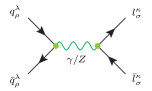
Figure 1: Feynman diagrams for the NC DY process at LO.

When we consider weak one-loop corrections to the parton-level LO NC DY process, $q\bar{q}\to\gamma,Z\to l^{+}l^{-}$, we refer to a correction of $\mathcal{O}(\alpha)$ involving only $W$ and $Z$ bosons in UV-divergent vertex and self-energy corrections, and UV-finite box corrections, as shown in Figs. 2, 3 and 4 respectively. The weak one-loop vertex corrections can be described by well-known form factors, $F^{\kappa}$ and $G^{\kappa}$, which multiply the LO vertex as schematically shown in Fig. 2.

Figure 2: Weak vertex corrections of $\mathcal{O}(\alpha)$ to the NC DY process $(V^{a}=Z,W)$.

The gauge-boson self-energy correction at ${\cal O}(\alpha)$ can also be factorized with respect to the LO amplitude as shown schematically in Fig. 3.

Figure 3: Gauge-boson self-energy correction at ${\cal O}(\alpha)$, where $\hat{\Sigma}_{T}^{V^{a}\bar{V}^{b}}$ is the renormalized vector boson self-energy, and $\Gamma_{V^{a}}$ the width of the gauge boson ($V^{a}=\gamma,Z)$. The red dot denotes the tree-level coupling to the initial ${\mathrm{q\bar{q}}}$ pair, $I^{V^{a}}_{q\bar{q}}$, and $I^{V^{b}}_{l\bar{l}}$ describes the coupling to the final lepton pair.

We implemented the explicit expressions of Ref. Hollik (1990) for the unrenormalized vector boson self-energies (Appendix A), the corresponding counterterms (Appendix B), and the renormalized form factor $\hat{F}^{\kappa}$ (Appendix C.1, Eq. (C.5)). For the renormalized form factor $\hat{G}^{\kappa}$ we use Eq. (3.13) of Ref. Beenakker et al. (1991). Note that the counterterms are defined in the on-shell renormalization scheme (see Refs. Hollik (1990); Beenakker et al. (1991) for details).

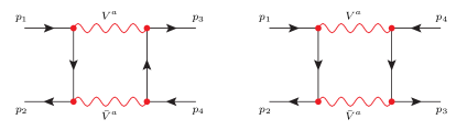
Figure 4: Feynman diagrams for weak one-loop box corrections to the NC DY process ($V^{a}=Z/W$).

The MCFM implementation of the weak one-loop box contributions due to the exchange of $Z/W^{\pm}$ bosons, shown in Fig. 4, represents our own calculation that expresses the results in terms of scalar integrals, which are evaluated with QCDLoop Ellis and Zanderighi (2008).

Finally, for the evaluation of the $Zf\bar{f}$ coupling at LO MCFM provides three choices of the EW input scheme, i.e. the so-called $\alpha(0)$, $\alpha(M_{Z}^{2})$, and $G_{\mu}$ schemes (see also Ref. Dittmaier and Huber (2010)). Note that the corrections relative to the LO cross section are always evaluated by using the fine-structure constant $\alpha(0)$. Also, in all three schemes the cosine of the weak mixing angle is defined via the physical $W$ and $Z$ masses as $\cos\theta_{W}=M_{W}/M_{Z}$ Sirlin (1980). When the form factors of the $Zf\bar{f}$ and $\gamma f\bar{f}$ vertices are renormalized in the $\alpha(0)$-scheme, the corrections depend on the light-fermion masses in a sensitive fashion due to terms proportional to $\alpha\log{m_{f}}$, which enter through electric charge renormalization in the on-shell scheme as Denner (1993)

$$\delta Z^{\mathrm{em}}_{e}=\mathrm{Re}\left(\frac{1}{2}\frac{\partial\Sigma^{\gamma}_{T}(k^{2})}{\partial k^{2}}\middle|_{k^{2}=0}\right)=\frac{2}{3}\frac{\alpha}{4\pi}\sum_{f\neq t}N_{\mathrm{C}}^{f}Q_{f}^{2}\log\left(\frac{M_{W}^{2}}{m_{f}^{2}}\right)+\ldots$$

The $\alpha(M_{Z}^{2})$-scheme introduces a contribution $\Delta\alpha(M_{Z}^{2})=-\mathrm{Re}\hat{\Pi}^{\gamma}(M_{Z}^{2})$ Denner (1993), where $\hat{\Pi}^{\gamma}(k^{2})=\Sigma_{T}^{\gamma}(k^{2})/k^{2}-2\delta Z^{\rm em}_{e}$ is the renormalized photon vacuum polarization, and the LO coupling is evaluated at $\alpha(M_{Z}^{2})=\alpha(0)/[1-\Delta\alpha(M_{Z}^{2})]$. Therefore, the relative corrections in the $\alpha(M_{Z}^{2})$-scheme absorb a term of $2~{}\Delta\alpha(M_{Z}^{2})$ resulting from the running of the electromagnetic coupling from $q^{2}=0$ to $q^{2}=M_{Z}^{2}$. As a result the logarithmic light-fermion terms are canceled at ${\cal O}(\alpha^{3})$.

The $G_{\mu}$-scheme implies the replacement $\alpha(0)\to\alpha_{G_{\mu}}$ with Sirlin (1980)

$$\alpha_{G_{\mu}}=\sqrt{2}G_{\mu}\frac{M_{W}^{2}(M_{Z}^{2}-M_{W}^{2})}{\pi M_{Z}^{2}}=\frac{\alpha(0)}{(1-\Delta r)}\;,$$ (5)

where $G_{\mu}$ is the Fermi constant measured in muon decay. The quantity $\Delta r$ describes the radiative corrections to muon decay, which is given at one-loop order by Sirlin (1980); Marciano and Sirlin (1980); Hollik (1990),

$$\Delta r^{\rm{1-loop}}=\Delta\alpha(M_{Z}^{2})-\frac{c_{w}^{2}}{s_{w}^{2}}\Delta\rho+\Delta r_{rem}=\frac{\hat{\Sigma}_{T}^{W}(0)}{M_{W}^{2}}+\frac{\alpha}{4\pi s_{\scriptscriptstyle{\mathrm{W}}}^{2}}\left(6+\frac{7-4s_{\scriptscriptstyle{\mathrm{W}}}^{2}}{4s_{\scriptscriptstyle{\mathrm{W}}}^{2}}\log c_{\scriptscriptstyle{\mathrm{W}}}^{2}\right)\;,$$ (6)

where $\hat{\Sigma}_{T}^{W}(0)$ is the renormalized $W$ boson self energy evaluated at $q^{2}=0$ and we have introduced the short-hand notation, $c_{\scriptscriptstyle{\mathrm{W}}}=\cos\theta_{W}$ and $s_{\scriptscriptstyle{\mathrm{W}}}=\sin\theta_{W}$. Note that $\Delta r$ contains $\Delta\alpha$, so that the relative correction in the $G_{\mu}$-scheme is also free of the logarithmic light-fermion mass dependence. Moreover, it also contains corrections to the $\rho$ parameter. We therefore recommend use of the $G_{\mu}$-scheme for obtaining precise predictions for the NC DY process, which is the default scheme in MCFM.

II.1.2 Top-quark pair production

Top-quark pairs are primarily produced through the strong interaction, which occurs at ${\cal O}(\alpha_{s}^{2})$ at LO. The LO diagrams are shown in Fig. 5, with gluon fusion representing approximately $90$% of the rate at the LHC and quark-antiquark annihilation the remainder.

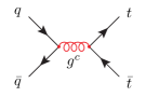
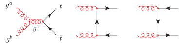
Figure 5: Feynman diagrams for LO strong ${\mathrm{t\bar{t}}}$ production at ${\cal O}(\alpha_{s}^{2})$.

We consider NLO weak corrections to the strong ${\mathrm{t\bar{t}}}$ production processes, i.e. we include all contributions of ${\cal O}(\alpha_{s}^{2}\alpha)$ to the cross sections of ${\mathrm{q\bar{q}}}$ annihilation and gluon fusion. This includes weak one-loop contributions of the form shown in Fig. 6 (for ${\mathrm{q\bar{q}}}$ annihilation) and Fig. 7 (for gluon fusion), as well as $s$-channel $Z,H$ exchange diagrams in the gluon fusion channel that are also shown in Fig. 7. For the MCFM implementation of the renormalized weak one-loop corrections to ${\mathrm{q\bar{q}}}$ annihilation and gluon fusion we have adopted the analytic expressions of Ref. Kühn et al. (2006) and Ref. Kühn et al. (2007), respectively. We have re-calculated the contributions from the $s$-channel $Z,H$ exchange diagrams. The UV poles in the vertex and self-energy corrections in both the ${\mathrm{q\bar{q}}}$ annihilation and gluon fusion subprocesses are removed by performing wave-function and top-mass renormalization in the on-shell renormalization scheme (see Refs. Beenakker et al. (1994); Kühn et al. (2006, 2007) for details). We have numerically cross-checked the implementation of the pure weak ${\cal O}(\alpha_{s}^{2}\alpha)$ contribution to ${\mathrm{t\bar{t}}}$ production against the calculation provided in Ref. Beenakker et al. (1994).

In the case of ${\mathrm{q\bar{q}}}$ annihilation, the ${\cal O}(\alpha_{s}^{2}\alpha)$ corrections include box diagrams that contain a gluon in the loop, specifically the gluon-$Z$ box diagram of Fig. 6 and the double-gluon box diagrams of Fig. 8. These contributions are UV finite but IR divergent.

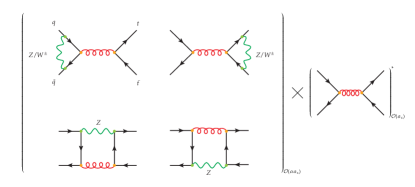
Figure 6: Sample diagrams for one-loop weak virtual corrections to the quark-antiquark annihilation subprocess in strong ${\mathrm{t\bar{t}}}$ production, which consist of vertex and box corrections, respectively. The $\hat{u}$-channel box diagrams are not explicitly shown.

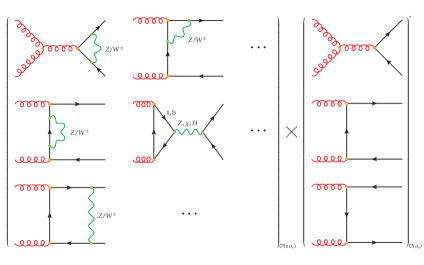
Figure 7: Sample diagrams for one-loop weak virtual corrections to the gluon fusion subprocess in strong ${\mathrm{t\bar{t}}}$ production, which consist of vertex, self-energy, and box corrections, respectively. The ellipses represent the vertex, self-energy and box diagrams which are not explicitly shown.

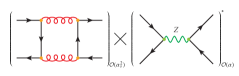
Figure 8: The contribution of the $\hat{t}$-channel two-gluon box diagram interfered with the $Z$-mediated Born diagram to the NLO cross section for ${\mathrm{t\bar{t}}}$ production at ${\cal O}(\alpha\alpha_{s}^{2})$. The contribution of the $\hat{u}$-channel two-gluon box diagram is not explicitly shown.

The IR divergences are canceled by the corresponding real gluon radiation contributions depicted in Fig. 9, as long as IR-safe observables are considered. In MCFM the extraction and cancellation of the IR poles is performed by using the Catani-Seymour dipole subtraction method Catani and Seymour (1997); Catani et al. (2002). Note that the color structure does not permit any contributions involving emitter and spectator partons that are either both in the initial state or both in the final state. The only dipole configurations that are present have one parton in the initial state and one in the final state. For completeness, the explicit expressions for the real contribution to ${\mathrm{t\bar{t}}}$ production at $\mathcal{O}(\alpha\alpha_{s}^{2})$, as implemented in MCFM, are provided in the appendix.

Figure 9: Sample diagrams for real corrections to ${\mathrm{t\bar{t}}}$ production in the ${\mathrm{q\bar{q}}}$ annihilation channel contributing to the ${\cal O}(\alpha\alpha_{s}^{2})$ cross section.

II.1.3 Di-jet production

Di-jet production is a ${\cal O}(\alpha_{s}^{2})$, ${\cal O}(\alpha^{2})$ or ${\cal O}(\alpha_{s}\alpha)$ process at LO, that is mediated by $2\to 2$ scattering processes involving light quarks and gluons, as shown in Fig. 10. The different subprocesses can be categorized in terms of the number of external quarks and gluons: four-quark, two-gluon-two-quark, and four-gluon subprocesses. In Tables 1 and 2 we list all processes of the four-quark and two-gluon-two-quark category. In practice it is only necessary to perform explicit calculations of each subprocess A listed in Tables 1 and 2, since all other processes can be obtained via crossing symmetry. The crossing relations are indicated in the tables. The four-gluon subprocess does not receive corrections at the order under consideration and thus only contributes to the LO cross section for di-jet production. Note that again we consider all external fermions to be massless and we do not include the $b$-quark-initiated processes.

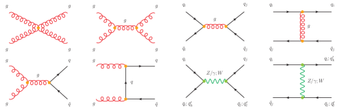
Figure 10: Sample tree-level Feynman diagrams for di-jet production via QCD and EW interactions.

Table 1: All four-quark subprocesses to di-jet production with the flavor indices $i,\,j$ so that $q_{i,j}\,\in\{\mathrm{u,d,c,s}\}$, where $i,\,j$ can be equal or different.

A.	$q_{i}\bar{q}_{i}\rightarrow q_{j}\bar{q}_{j}$, direct calculation
B.	$q_{i}q_{j}\rightarrow q_{i}q_{j}$, $(2\rightarrow 3,\,3\rightarrow 4,\,4\rightarrow 2;\,s\rightarrow t,\,t\rightarrow u,\,u\rightarrow s)$
C.	$\bar{q}_{i}q_{i}\rightarrow\bar{q}_{j}q_{j}$, $(1\leftrightarrow 2,3\leftrightarrow 4)$
D.	$\bar{q}_{i}\bar{q}_{j}\rightarrow\bar{q}_{i}\bar{q}_{j}$, $(1\rightarrow 3,\,3\rightarrow 2,\,2\rightarrow 1;\,s\rightarrow t,\,t\rightarrow u,\,u\rightarrow s)$
E.	$q_{i}\bar{q}_{j}\rightarrow q_{i}\bar{q}_{j}$, $(2\leftrightarrow 3;\,s\leftrightarrow t)$
F.	$\bar{q}_{i}q_{j}\rightarrow\bar{q}_{i}q_{j}$, $(1\rightarrow 3,\,3\rightarrow 4,\,4\rightarrow 2,\,2\rightarrow 1;\,s\leftrightarrow t)$

Table 2: All two-gluon-two-quark subprocesses to di-jet production, where $q\in\{\mathrm{u,d,c,s}\}$. Note that the amplitude is multiplied by a minus sign when crossing a final/initial state quark to an initial/final state one.

A.	$gg\rightarrow q\bar{q}$, direct calculation
B.	$gq\rightarrow gq$, $(2\rightarrow 3,3\rightarrow 4,4\rightarrow 2;\,s\rightarrow t,t\rightarrow u,u\rightarrow s)$
C.	$g\bar{q}\rightarrow g\bar{q}$, $(2\leftrightarrow 3;\,s\leftrightarrow t)$
D.	$qg\rightarrow qg$, $(1\leftrightarrow 4;\,s\leftrightarrow t)$
E.	$\bar{q}g\rightarrow\bar{q}g$, $(1\rightarrow 2,\,2\rightarrow 4,4\rightarrow 3,\,3\rightarrow 1;\,s\leftrightarrow t)$
F.	$q\bar{q}\rightarrow gg$, $(1\leftrightarrow 3,\,2\leftrightarrow 4;\,t\leftrightarrow u)$
G.	$\bar{q}q\rightarrow gg$ $(1\leftrightarrow 4,\,2\leftrightarrow 3)$

The one-loop corrections to di-jet production at fixed $\mathcal{O}(\alpha\alpha_{s}^{2})$ consist of $\mathcal{O}(\alpha)$ corrections to the QCD mediated processes interfered with the LO ${\cal O}(\alpha_{s})$ amplitudes and of $\mathcal{O}(\alpha_{s})$ corrections to the QCD(weak) mediated processes interfered with the LO $\mathcal{O}(\alpha)(\mathcal{O}(\alpha_{s}))$ amplitudes. Their contributions to the partonic di-jet cross section at $\mathcal{O}(\alpha\alpha_{s}^{2})$ can be written symbolically as

$$d\hat{\sigma}(\alpha_{s}^{2}\alpha) \propto 2\mathrm{Re}\left[\delta\mathcal{M}(\alpha_{s}\alpha)\cdot\mathcal{M}_{0}^{*}(\alpha_{s})+\delta\mathcal{M}(\alpha_{s}^{2})\cdot\mathcal{M}_{0}^{*}(\alpha)\right]$$ (7)

where $\mathcal{M}_{0}(\alpha_{s})$ and $\mathcal{M}_{0}(\alpha)$ denote the LO amplitude with gluon and weak boson exchange, respectively. $\delta\mathcal{M}(\alpha_{s}^{2})$ denotes the QCD one-loop correction to the strong LO amplitude while $\delta\mathcal{M}(\alpha_{s}\alpha)$ represents both weak corrections to the strong LO amplitude and QCD corrections to the weak LO amplitude. As was the case for ${\mathrm{t\bar{t}}}$ production, we also need to take into account real QCD corrections in order to cancel the IR divergences stemming from the virtual QCD corrections. Explicit expressions for the real corrections can be found in the appendix. In the following we will present the virtual corrections to the four-quark and two-gluon-two-quark subprocesses, $q_{i}\bar{q}_{i}\rightarrow q_{j}\bar{q}_{j}$ and $gg\rightarrow q\bar{q}$. All remaining subprocesses can be obtained via the crossing relations listed in Table 1 and 2. The virtual corrections to the two-gluon-two-quark subprocess $gg\rightarrow q\bar{q}$ consist of the same weak one-loop corrections as in ${\mathrm{t\bar{t}}}$ production, shown in Fig. 7, with the top quark replaced by a massless quark. For other subprocesses we have partially used the analytic expressions for the weak corrections to $b$-jet production of Ref. Kühn et al. (2010), where applicable to the case of di-jet production.

Table 3: The three categories of subprocesses that comprise the four-quark processes $q_{i}\bar{q}_{i}\rightarrow q_{j}\bar{q}_{j}$ of di-jet production (with $u_{1,2}=u,c$ and $d_{1,2}=d,s$).

category 1	$u_{i}\bar{u}_{i}\rightarrow u_{j}\bar{u}_{j},d_{i}\bar{d}_{i}\rightarrow d_{j}\bar{d}_{j}\,,\,\mbox{ for}~{}i\neq j$
category 2	$u_{i}\bar{u}_{i}\rightarrow d_{j}\bar{d}_{j},d_{i}\bar{d}_{i}\rightarrow u_{j}\bar{u}_{j}$
category 3	$u_{i}\bar{u}_{i}\rightarrow u_{i}\bar{u}_{i},d_{i}\bar{d}_{i}\rightarrow d_{i}\bar{d}_{i}$

In the case of the four-quark subprocesses $q_{i}\bar{q}_{i}\rightarrow q_{j}\bar{q}_{j}$ we further divide them into the three categories shown in Table 3 since, as discussed further shortly, they proceed through different diagrams. The virtual corrections to the four-quark subprocesses of category 1 of Table 3 can again be obtained from the weak corrections to ${\mathrm{t\bar{t}}}$ production shown in Fig. 6. Sample diagrams for virtual corrections to the four-quark subprocesses of category 2 and 3 of Table 3 are shown in Fig. 11 and Fig. 12, respectively. While the color structure ensures that there is no contribution from the interference between one-loop QCD and LO weak diagrams in category 1 (except for the mixed QCD-weak box contribution), such corrections do survive in category 2 (diagrams below the double line in Fig. 11) and category 3 (Fig. 12).

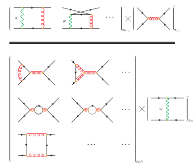
Figure 11: Sample Feynman diagrams for virtual corrections to four-quark subprocesses of category 2 of Table 3, $u_{i}\bar{u}_{i}\rightarrow d_{j}\bar{d}_{j}$, $d_{i}\bar{d}_{i}\rightarrow u_{j}\bar{u}_{j}$, where $i,\,j$ denote the $i$th- or $j$th-generation of the light (anti)quarks, i.e, $i,\,j\in(1,2)$. The diagrams above the double line contribute to $\delta\mathcal{M}(\alpha_{s}\alpha)$ and below the double line to $\delta\mathcal{M}(\alpha_{s}^{2})$. Weak one-loop corrections similar to the ones shown in Fig. 6 are not explicitly shown.

Figure 12: Sample Feynman diagrams for virtual corrections to four-quark subprocesses of category 3 of Table 3, $q\bar{q}\rightarrow q\bar{q}$, $q\in\{u_{i},d_{i}\}$. Contributions similar to the ones shown in Fig. 6 and 11 are not explicitly shown.

The UV poles in self-energy and vertex corrections are eliminated after applying an appropriate renormalization procedure as described below. The IR poles originating from the soft and collinear virtual gluon contributions in category 2 and 3 are canceled against their counterparts from the real corrections and PDF counterterms as described in the appendix. Note that these real QCD corrections yield real corrections to the quark-gluon-initiated subprocesses of Table 2 by crossing the emitted gluon to the initial state. These corrections exhibit a trivial initial-state collinear singularity which is absorbed into the PDFs (as detailed in the appendix).

The weak one-loop vertex corrections in all three categories involve $Z/W^{\pm}$ boson exchange in the $gq\bar{q}$ vertex, which can be described in terms of the renormalized form factor $f_{1}$ given in Eq. (III.11) of Ref. Kühn et al. (2010) (or (II.16) of Ref. Kühn et al. (2006)), as

$$\delta\mathcal{M}\left(\alpha_{s}\alpha\right)_{y}=-\frac{1}{2}\frac{\alpha}{4\pi}\mathcal{M}_{0}\left(\alpha_{s}\right)_{y}\left\{\sum_{f=q_{i},q_{j}}\left[\left(g_{v}^{f}\right)^{2}+\left(g_{a}^{f}\right)^{2}\right]f_{1}\left(\frac{M_{Z}^{2}}{y}\right)+\frac{1}{2s_{w}^{2}}f_{1}\left(\frac{M_{W}^{2}}{y}\right)\;,\right\}$$ (8)

where $g_{v}^{f}(g_{a}^{f})$ is the vector(axial) vector coupling of the fermion to the $Z$ boson, $g_{v}^{f}=1/(2s_{w}c_{w})(T_{3}^{f}-2s_{w}^{2}Q_{f}),g_{a}^{f}=1/(2s_{w}c_{w})T^{3}_{f}$, and the subscript $y$ denotes the channel of the amplitude, while the variable $y$ in the function $f_{1}$ denotes the Mandelstam variable corresponding to that channel. The function $f_{1}$ is given by

$$f_{1}(x)=1+2\left[\left(1+\log(x)\right)\left(2x+3\right)-2\left(1+x\right)^{2}\left(\mathrm{Li}_{2}\left(1+\frac{1}{x}\right)-\frac{\pi^{2}}{6}\right)\right].$$ (9)

The renormalized contribution of the QCD vertex and self-energy corrections in category 2 and 3 to $d\hat{\sigma}$ can be written as

$$\delta\mathcal{M}\left(\alpha_{s}^{2}\right)_{x}=\frac{\alpha_{s}}{4\pi}\mathcal{M}_{0}\left(\alpha_{s}\right)_{x}\left[2\Lambda_{1}(x)+2\Lambda_{2}(x)+\Pi(x)+\delta Z_{g_{s}}\right]$$ (10)

where the subscript and variable $x$ have the same interpretation as $y$ in Eq. (8), and $\delta Z_{g_{s}}$ denotes the renormalization constant for the strong coupling

$$\delta Z_{g_{s}}=\left[\left(-\frac{11}{2}+\frac{n_{F}}{3}\right)\frac{1}{\epsilon}+\frac{1}{3}\left(\frac{1}{\epsilon}+\log\frac{\mu^{2}}{m_{t}^{2}}\right)\right]\;,$$ (11)

where $m_{t}$ denotes the top-quark mass, $d=4-2\epsilon$ and we do not distinguish between IR and UV poles. Consequently, the quark wave function renormalization constant $\delta Z_{q}=-\alpha_{s}/(3\pi)B_{0}(0,0,0)\equiv 0$. The two form factors $\Lambda_{1}$ and $\Lambda_{2}$, describing virtual gluon corrections to $gq\bar{q}$ and $V^{a}q\bar{q}$ ($V^{a}=Z,\gamma,W^{\pm}$) vertices respectively, read

$$\Lambda_{1}(x) = \frac{1-N_{\mathrm{c}}^{2}}{4N_{\mathrm{c}}}\left[\left(d-7\right)~{}B_{0}\left(x,0,0\right)-2~{}x~{}C_{0}\left(0,x,0,0,0,0\right)\right]-\frac{N_{\mathrm{c}}\left(N_{\mathrm{c}}^{2}-1\right)}{4}B_{0}\left(x,0,0\right)$$ (12)

$$\Lambda_{2}(x) = \frac{\left(N_{\mathrm{c}}^{2}-1\right)^{2}}{4N_{\mathrm{c}}}\left[\left(d-7\right)~{}B_{0}\left(x,0,0\right)-2~{}x~{}C_{0}\left(0,x,0,0,0,0\right)\right],$$ (13)

with the scalar integrals

$$B_{0}(x,0,0)=\frac{1}{\epsilon}+\log\frac{\mu^{2}}{-x-i\varepsilon}+2+\mathcal{O}\left(\epsilon\right)$$

$$C_{0}(0,x,0,0,0,0)=\frac{1}{x}\left[\frac{1}{\epsilon^{2}}+\frac{1}{\epsilon}\log\frac{\mu^{2}}{-x-i\varepsilon}+\frac{1}{2}\log^{2}\frac{\mu^{2}}{-x-i\varepsilon}\right]+\mathcal{O}\left(\epsilon\right)\,.$$

Finally, the gluon self-energy correction reads

$$\Pi(x)=\frac{1}{2(d-1)} \big{[}4(d-2)~{}A_{0}\left(m_{t}^{2}\right)+\left(9d-6-2(d-2)n_{F}\right)~{}x~{}B_{0}\left(x,0,0\right)$$ (14)

$$-2~{}\left(4m_{t}^{2}+(d-2)x\right)~{}B_{0}\left(x,m_{t}^{2},m_{t}^{2}\right)\big{]},$$

with

$$A_{0}\left(m_{t}^{2}\right)=m_{t}^{2}\left[\frac{1}{\epsilon}+1+\log\frac{\mu^{2}}{m_{t}^{2}-i\varepsilon}\right]+\mathcal{O}\left(\epsilon\right)$$

$$B_{0}\left(x,m_{t}^{2},m_{t}^{2}\right)=\frac{1}{\epsilon}+2+\log\frac{\mu^{2}}{m_{t}^{2}}-\sqrt{1-\frac{4m_{t}^{2}}{x}}\log\frac{1+\sqrt{1-\frac{4m_{t}^{2}}{x}}}{-1+\sqrt{1-\frac{4m_{t}^{2}}{x}}}+\mathcal{O}\left(\epsilon\right)$$

Depending on the production channel considered, the variable $x$ could be $\hat{s}$, $\hat{t}$, or $\hat{u}$.

The box contributions to $d\hat{\sigma}$ can be written in terms of four contributions for all di-jet subprocesses, by taking advantage of appropriate crossing relations. In this way, $d\hat{\sigma}$ can be schematically written as

$$d\hat{\sigma}=4\pi\alpha\alpha_{s}^{2} \Big{\{}\mathrm{prop}_{V^{a}}\left(x\right)[cs_{1}(\Box^{{\mathrm{t\times s}}}+\Box^{{\mathrm{u\times s}}})+cs_{2}(\Box^{{\mathrm{t\times t}}}+\Box^{{\mathrm{u\times t}}})](M_{V^{a}}\neq 0)$$ (15)

$$\qquad\qquad+(cs_{1}(\Box^{{\mathrm{t\times s}}}+\Box^{{\mathrm{u\times s}}})+cs_{2}\Box^{{\mathrm{u\times t}}}+cs_{3}\Box^{{\mathrm{t\times t}}})(M_{V^{a}}=0)\Big{\}}$$

in terms of the three possible color factors

$$cs_{1}=\frac{N_{\mathrm{c}}^{2}-1}{4},\quad cs_{2}=\frac{-N_{\mathrm{c}}^{2}+1}{4N_{\mathrm{c}}},\quad cs_{3}=\frac{\left(N_{\mathrm{c}}^{2}-1\right)^{2}}{4N_{\mathrm{c}}}$$

and the propagator function defined by

$$\mathrm{prop}_{V^{a}}\left(x\right)=\frac{x\left(x-M_{V^{a}}^{2}\right)}{\left(x-M_{V^{a}}^{2}\right)^{2}+\Gamma_{V^{a}}^{2}M_{V^{a}}^{2}}$$ (16)

The integral functions for the interference of the $t$-channel and $u$-channel box diagrams with the $s$-channel and $t$-channel LO diagrams, $\Box^{{\mathrm{t\times s}}}$, $\Box^{{\mathrm{u\times s}}}$ and $\Box^{{\mathrm{t\times t}}}$, $\Box^{{\mathrm{u\times t}}}$, respectively, are given by

$$\Box^{{\mathrm{t\times s}}}= \frac{8}{\hat{s}}\bigg{\{}-\left(g_{a}^{f}g_{a}^{i}+g_{v}^{f}g_{v}^{i}\right)\left[2\hat{u}\left(B_{0}\left(\hat{s},M_{V^{a}}^{2}\right)-B_{0}\left(\hat{t},0\right)\right)+\hat{t}(M_{V^{a}}^{2}+\hat{t}-\hat{u})\left(C_{0}^{1}\left(\hat{t},M_{V^{a}}^{2}\right)+C_{0}^{2}\left(\hat{t},0\right)\right)\right]$$ (17)

$$+2\left(g_{a}^{f}g_{a}^{i}\left(\hat{t}+\hat{u}\right)\left(M_{V^{a}}^{2}-\hat{t}+\hat{u}\right)+g_{v}^{f}g_{v}^{i}\left(M_{V^{a}}^{2}\left(\hat{t}+\hat{u}\right)+3\hat{t}^{2}+\hat{u}^{2}\right)\right)C_{0}^{2}\left(\hat{s},M_{V^{a}}^{2}\right)$$

$$+\hat{t}\left(-g_{a}^{f}g_{a}^{i}\left(M_{V^{a}}^{4}+2M_{V^{a}}^{2}\hat{t}-\hat{t}^{2}+\hat{u}^{2}\right)-g_{v}^{f}g_{v}^{i}\left(M_{V^{a}}^{4}+2M_{V^{a}}^{2}\hat{t}+3\hat{t}^{2}+\hat{u}^{2}\right)\right)D_{0}\left(\hat{s},\hat{t},M_{V^{a}}^{2}\right)\bigg{\}}$$

$$\Box^{{\mathrm{u\times s}}}= \frac{8}{\hat{s}}\bigg{\{}-\left(g_{a}^{f}g_{a}^{i}-g_{v}^{f}g_{v}^{i}\right)\left[2\hat{t}\left(B_{0}\left(\hat{s},M_{V^{a}}^{2}\right)-B_{0}\left(\hat{u},0\right)\right)+\hat{u}\left(M_{V^{a}}^{2}-\hat{t}+\hat{u}\right)\left(C_{0}^{1}\left(\hat{u},M_{V^{a}}^{2}\right)+C_{0}^{2}\left(\hat{u},0\right)\right)\right]$$ (18)

$$+2\left(g_{a}^{f}g_{a}^{i}\left(\hat{t}+\hat{u}\right)\left(M_{V^{a}}^{2}+\hat{t}-\hat{u}\right)-g_{v}^{f}g_{v}^{i}\left(M_{V^{a}}^{2}\left(\hat{t}+\hat{u}\right)+\hat{t}^{2}+3\hat{u}^{2}\right)\right)C_{0}^{2}\left(\hat{s},M_{V^{a}}^{2}\right)$$

$$+\hat{u}\left(-g_{a}^{f}g_{a}^{i}\left(M_{V^{a}}^{4}+2M_{V^{a}}^{2}\hat{u}+\hat{t}^{2}-\hat{u}^{2}\right)+g_{v}^{f}g_{v}^{i}\left(M_{V^{a}}^{4}+2M_{V^{a}}^{2}\hat{u}+\hat{t}^{2}+3\hat{u}^{2}\right)\right)D_{0}\left(\hat{s},\hat{u},M_{V^{a}}^{2}\right)\bigg{\}}$$

$$\Box^{{\mathrm{t\times t}}}= -\frac{8}{\hat{t}}\left(g_{a}^{f}g_{a}^{i}+g_{v}^{f}g_{v}^{i}\right)\big{[}2\hat{u}\left(B_{0}(\hat{s},M_{V^{a}}^{2})-B_{0}(\hat{t},0)\right)+\hat{t}\left(M_{V^{a}}^{2}+\hat{t}-\hat{u}\right)\left(C_{0}^{1}(\hat{t},M_{V^{a}}^{2})+C_{0}^{2}(\hat{t},0)\right)$$ (19)

$$-2\left(M_{V^{a}}^{2}\left(\hat{t}+\hat{u}\right)+\hat{t}^{2}+\hat{u}^{2}\right)C_{0}^{2}\left(\hat{s},M_{V^{a}}^{2}\right)$$

$$+\hat{t}\left(M_{V^{a}}^{4}+2M_{V^{a}}^{2}\hat{t}+\hat{t}^{2}+\hat{u}^{2}\right)D_{0}\left(\hat{s},\hat{t},M_{V^{a}}^{2}\right)\big{]}$$

$$\Box^{{\mathrm{u\times t}}}=\frac{16\hat{u}^{2}}{\hat{t}}(g_{a}^{f}g_{a}^{i}+g_{v}^{f}g_{v}^{i})(\hat{u}D_{0}(\hat{s},\hat{u},M_{V^{a}}^{2})-2C_{0}^{2}(\hat{s},M_{V^{a}}^{2}))$$ (20)

In these expressions we have used the short-hand notation

$$B_{0}\left(x,y\right)=B_{0}\left(x,y,0\right)$$

$$C_{0}^{1}\left(x,y\right)=C_{0}\left(x,0,0,0,0,y\right)$$

$$C_{0}^{2}\left(x,y\right)=C_{0}\left(x,0,0,0,y,0\right)$$

$$D_{0}\left(x,y,z\right)=D_{0}\left(0,0,0,0,x,y,z,0,0,0\right)$$

for the scalar integrals, which read

$$B_{0}\left(x,y\right)=\left\{\begin{array}[]{lr}\frac{1}{\epsilon}+2+\log\frac{\mu^{2}}{-x}&(y=0\;||\;y=x)\\ \frac{1}{\epsilon}+2+\frac{y-x}{x}\log\frac{y-x}{y}+\log\frac{\mu^{2}}{y}&\mathrm{otherwise}\end{array}\right.$$ (21a)

$$C_{0}^{1}\left(x,y\right)=\left\{\begin{array}[]{lr}\frac{1}{x}\mathrm{Li}_{2}\left(1\right)=\frac{\pi^{2}}{6x}&(y=-x)\\ C_{0}^{2}\left(x,0\right)&(y=0)\\ \frac{1}{x}\left[\log\left(-\frac{x}{y}\right)\log\left(1+\frac{x}{y}\right)+\mathrm{Li}_{2}\left(-\frac{x}{y}\right)\right]&\mathrm{otherwise}\end{array}\right.$$ (21b)

$$C_{0}^{2}\left(x,y\right)=\left\{\begin{array}[]{lr}\frac{1}{x}\left[\frac{1}{\epsilon^{2}}+\frac{1}{\epsilon}\log\frac{\mu^{2}}{-x}+\frac{1}{2}\log^{2}\frac{\mu^{2}}{-x}\right]&(y=0)\\ -\frac{1}{2x}\left[\frac{1}{\epsilon^{2}}+\frac{1}{\epsilon}\log\frac{\mu^{2}}{y}+\frac{\pi^{2}}{6}+\frac{1}{2}\log^{2}\frac{\mu^{2}}{y}\right]&(y=x)\\ \frac{1}{x}\left[\frac{1}{\epsilon}\log\frac{y}{y-x}+\log^{2}\frac{y}{y-x}+\log\frac{\mu^{2}}{y}\log\frac{y}{y-x}+\mathrm{Li}_{2}\left(\frac{x}{y}\right)\right]&\mathrm{otherwise}\end{array}\right.$$ (21c)

$$D_{0}\left(x,y,z\right)=\left\{\begin{array}[]{ll}\frac{1}{xy}\left[\frac{4}{\epsilon^{2}}+\frac{2}{\epsilon}\left(\log\frac{\mu^{2}}{-x}+\log\frac{\mu^{2}}{y}\right)+\log^{2}\frac{\mu^{2}}{-x}+\log^{2}\frac{\mu^{2}}{y}-\log^{2}\frac{x}{y}-\pi^{2}\right]&(z=0)\\ \frac{1}{(x-z)y}\Big{[}\frac{1}{\epsilon^{2}}+\frac{1}{\epsilon}\left(\log\frac{\mu^{2}}{y}+2\log\frac{z}{z-x}\right)+\frac{1}{2}\log^{2}\frac{\mu^{2}}{-y}-\frac{1}{2}\log^{2}\frac{z}{-y}\\ \qquad+2\log\frac{\mu^{2}}{-y}\log\frac{z}{z-x}-4~{}\mathrm{Li}_{2}\left(\frac{x}{x-z}\right)-\mathrm{Li}_{2}\left(1+\frac{z}{y}\right)-\frac{\pi^{2}}{6}\Big{]}&(z\neq 0)\end{array}\right.$$ (21d)

Here $g_{v}^{f},g_{a}^{f}$ parameterize both the coupling of the fermion to the $Z$ and $W$ boson (with $g_{v}=g_{a}=1/(2\sqrt{2}s_{w})$ in the $W$ case). It should be noted that the third expression in Eq. (21b) is exact only for $-|y|<x<0$, otherwise there is a phase difference that we have omitted here. Since only the real part contributes to $d\hat{\sigma}$ it would not alter the final result. For $M_{V^{a}}>0$, the expressions in Eqs. (17)-(20) describe box diagrams with a gluon and a massive vector boson, while for $M_{V^{a}}=0$, they describe the pure QCD box diagrams with two gluons. As in ${\mathrm{t\bar{t}}}$ production, we differentiate between them as weak box and QCD box contributions respectively.

II.2 Leading and Subleading Logarithms in the Sudakov regime

As discussed earlier, the NLO EW corrections at high energies are dominated by logarithms of $\hat{s}_{ij}/M_{V^{a}}^{2}$, where $\hat{s}_{ij}=(p_{i}+p_{j})^{2}$ are Mandelstam variables of momenta $p_{i},~{}\;p_{j}$ associated with external particles $i,\,j$, and $M_{V^{a}}$ is the mass of the weak gauge boson $V^{a}=Z,W$.

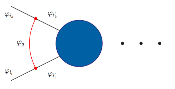
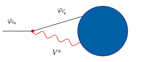
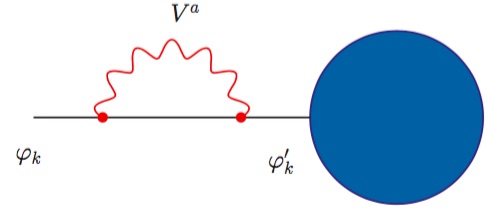
Figure 13: Feynman diagrams representing soft-collinear contributions resulting in double logarithms (left), collinear contributions (middle) and contributions from wave function renormalization (right) both resulting in single logarithms.

For the implementation of the weak leading and subleading logarithms at one-loop in MCFM we adopt the formalism of Refs. Denner and Pozzorini (2001a, b). As described in detail in Ref. Denner and Pozzorini (2001b), the ${\cal O}(\alpha)$ corrections to a $2\to 2$ process in logarithmic approximation (LA) in the Sudakov regime, i. e. when all Mandelstam variables are of the same size and are much larger than the weak scale, $|\hat{s}_{ij}|~{}\sim~{}\hat{s}\gg M_{W}^{2}$, factorize into the Born amplitude and double (DL) and single logarithms (SL). The double logarithms $\log^{2}(\hat{s}_{kl}/M_{V^{a}}^{2})$ originate from the soft-collinear contributions due to the exchange of virtual EW gauge bosons between external legs $k,l$, as illustrated in Fig. 13 (left). The possible sources of single logarithms in virtual EW corrections are collinear mass singularities and wave-function and parameter renormalization when the UV singularities are subtracted at $\mu_{R}\approx M_{V^{a}}$. The contributions of collinear radiation and wave-function renormalization are schematically shown in Fig. 13 (middle and left). Thus, in the LA limit the ${\cal O}(\alpha)$ corrections to the LO amplitude $\mathcal{M}_{0}$ can be written as

$$\delta\mathcal{M}=\frac{\alpha}{4\pi}\left(\delta^{\mathrm{LSC}}+\delta^{\mathrm{SSC}}+\delta^{\mathrm{C}}+\delta^{\mathrm{PR}}\right)\mathcal{M}_{0}\;,$$ (22)

where $\delta^{\mathrm{LSC}}$ and $\delta^{\mathrm{SSC}}$ denote respectively the leading and sub-leading logarithms of soft-collinear origin, $\delta^{\mathrm{C}}$ the collinear logarithms and $\delta^{\mathrm{PR}}$ the logarithms originating from parameter renormalization. For completeness, we provide in the following the explicit expressions for $\delta^{\mathrm{LSC,SSC,C,PR}}$ and $\mathcal{M}_{0}$ for the NC DY process, $t\bar{t}$ and di-jet production, as they are implemented in MCFM. For the details of their derivation we refer to Refs. Denner and Pozzorini (2001a, b).

II.2.1 Neutral-Current Drell-Yan Process

The LO amplitude in LA for a given fermion chirality $\tau,\lambda=\mathrm{L},\mathrm{R}$ and isospin index $\rho,\sigma$ reads

$$\mathcal{M}^{q_{\rho}^{\tau}l_{\sigma}^{\lambda}}_{0}=4\pi\alpha R_{q_{\rho}^{\tau}l_{\sigma}^{\lambda}}\frac{\mathcal{A}_{\tau\lambda}}{\hat{s}}$$ (23)

where

$$R_{q_{\rho}^{\tau}l_{\sigma}^{\lambda}}=\sum_{N=Z,\gamma}I_{q_{\rho}^{\tau}}^{N}I_{l_{\sigma}^{\lambda}}^{N}=\frac{Y_{q_{\rho}^{\tau}}Y_{l_{\sigma}^{\lambda}}}{4c_{\scriptscriptstyle{\mathrm{W}}}^{2}}+\frac{T^{3}_{q_{\rho}^{\tau}}T^{3}_{l_{\sigma}^{\lambda}}}{s_{\scriptscriptstyle{\mathrm{W}}}^{2}}$$

and $Y$ and $T^{3}$ are the hypercharge and 3rd-component of the weak isospin $T$, respectively, which are related to the electric charge $Q$ via the Gell-Mann-Nishijima formula $Q=Y/2+T^{3}$. The LO amplitude for each chirality combination $\mathcal{A}_{\tau\lambda}$ is $\mathcal{A}_{\mathrm{L}\mathrm{L}}=\mathcal{A}_{\mathrm{R}\mathrm{R}}=\hat{u}$, and $\mathcal{A}_{\mathrm{L}\mathrm{R}}=\mathcal{A}_{\mathrm{R}\mathrm{L}}=\hat{t}$. After removing the photonic virtual corrections from the expressions provided in Ref. Denner and Pozzorini (2001b), the different contributions in Eq. (22) read,

$$\delta^{\mathrm{LSC}}_{q_{\rho}^{\tau}l_{\sigma}^{\lambda}}=-\left(C^{{\mathrm{wk}}}_{q_{\rho}^{\tau}}+C^{{\mathrm{wk}}}_{l_{\sigma}^{\lambda}}\right)\log^{2}\left(\frac{\hat{s}}{M_{W}^{2}}\right)+2\log\left(\frac{M_{Z}^{2}}{M_{W}^{2}}\right)\left[\left(I^{Z}_{q_{\rho}^{\tau}}\right)^{2}+\left(I^{Z}_{l_{\sigma}^{\lambda}}\right)^{2}\right]\log\left(\frac{\hat{s}}{M_{W}^{2}}\right),$$ (24)

$$\begin{aligned} \delta^{\mathrm{SSC}}_{q_{\rho}^{\tau}l_{\sigma}^{\lambda}}=&-4\left[\log\left(\frac{\hat{s}}{M_{W}^{2}}\right)-\log\left(\frac{M_{Z}^{2}}{M_{W}^{2}}\right)\right]R_{q_{\rho}^{\tau}l_{\sigma}^{\lambda}}\left(I^{Z}_{q_{\rho}^{\tau}}I^{Z}_{l_{\sigma}^{\lambda}}\right)\log\left(\frac{\hat{t}}{\hat{u}}\right)\\ &-\frac{\delta_{\tau\mathrm{L}}\delta_{\lambda\mathrm{L}}}{s_{\scriptscriptstyle{\mathrm{W}}}^{4}R_{q_{\rho}^{\tau}l_{\sigma}^{\lambda}}}\log\left(\frac{\hat{s}}{M_{W}^{2}}\right)\left[\delta_{\rho\sigma}\log\left(\frac{|\hat{t}|}{\hat{s}}\right)-\delta_{-\rho\sigma}\log\left(\frac{|\hat{u}|}{\hat{s}}\right)\right].\end{aligned}$$

$$\delta^{\mathrm{C}}_{q_{\rho}^{\tau}l_{\sigma}^{\lambda}}=3\left(C^{{\mathrm{wk}}}_{q_{\rho}^{\tau}}+C^{{\mathrm{wk}}}_{l_{\sigma}^{\lambda}}\right)\log\left(\frac{\hat{s}}{M_{W}^{2}}\right)$$ (25)

$$\delta^{\mathrm{PR}}_{q_{\rho}^{\tau}l_{\sigma}^{\lambda}}=\left(\frac{s_{\scriptscriptstyle{\mathrm{W}}}}{c_{\scriptscriptstyle{\mathrm{W}}}}b^{\mathrm{ew}}_{\mathrm{AZ}}\Delta_{q^{\tau}_{\rho}l^{\lambda}_{\sigma}}-b^{\mathrm{ew}}_{\mathrm{AA}}\right)\log\left(\frac{\hat{s}}{M_{W}^{2}}\right)$$ (26)

$${\rm with} \Delta_{q^{\tau}_{\rho}l^{\lambda}_{\sigma}}:=\frac{-\frac{1}{4c_{\scriptscriptstyle{\mathrm{W}}}^{2}}Y_{q^{\tau}_{\rho}}Y_{l^{\lambda}_{\sigma}}+\frac{c_{\scriptscriptstyle{\mathrm{W}}}^{2}}{s_{\scriptscriptstyle{\mathrm{W}}}^{4}}T^{3}_{q^{\tau}_{\rho}}T^{3}_{l^{\lambda}_{\sigma}}}{R_{q_{\rho}^{\tau}l_{\sigma}^{\lambda}}},\;b^{\mathrm{ew}}_{AZ}=-\frac{19+22s_{\scriptscriptstyle{\mathrm{W}}}^{2}}{6s_{\scriptscriptstyle{\mathrm{W}}}c_{\scriptscriptstyle{\mathrm{W}}}},\;\;\;b^{\mathrm{ew}}_{AA}=-\frac{11}{3}.$$

$C^{{\mathrm{wk}}}_{f^{\kappa}}$ is defined in terms of the electroweak Casimir operator as $C^{{\mathrm{wk}}}_{f^{\kappa}}=C^{ew}_{f^{\kappa}}-Q_{f^{\kappa}}^{2}$ and

$$I^{Z}_{f^{\kappa}}=\frac{T^{3}_{f^{\kappa}}-s_{\scriptscriptstyle{\mathrm{W}}}^{2}Q_{f^{\kappa}}}{s_{\scriptscriptstyle{\mathrm{W}}}c_{\scriptscriptstyle{\mathrm{W}}}}.$$

Explicit expressions for $C^{ew}_{f^{\kappa}}$ can be found in Appendix B of Ref. Denner and Pozzorini (2001b).

II.2.2 Top-quark Pair Production

The weak ${\cal O}(\alpha)$ corrections in LA to the LO amplitudes for the quark-antiquark annihilation and gluon fusion channels again consist of the different contributions in Eq. (22) which read

$$\delta^{\mathrm{LSC}}_{q_{1}^{\tau}q_{2}^{\lambda}}=-\left(C^{{\mathrm{wk}}}_{q_{1}^{\tau}}+C^{{\mathrm{wk}}}_{q_{2}^{\lambda}}\right)\log^{2}\left(\frac{\hat{s}}{M_{W}^{2}}\right)+2\log\left(\frac{M_{Z}^{2}}{M_{W}^{2}}\right)\left[\left(I^{Z}_{q_{2}^{\lambda}}\right)^{2}+\left(I^{Z}_{q_{2}^{\lambda}}\right)^{2}\right]\log\left(\frac{\hat{s}}{M_{W}^{2}}\right),$$ (27)

$$\begin{aligned} \delta^{\mathrm{SSC}}_{q_{1}^{\tau}q_{2}^{\lambda}}=&-4\left[\log\left(\frac{\hat{s}}{M_{W}^{2}}\right)-\log\left(\frac{M_{Z}^{2}}{M_{W}^{2}}\right)\right]\left(I^{Z}_{q_{1}^{\tau}}I^{Z}_{q_{2}^{\lambda}}\right)\log\left(\frac{\hat{t}}{\hat{u}}\right)\,\delta_{q_{1}q}\end{aligned}$$

$$\delta^{\mathrm{C}}_{q_{1}^{\tau}q_{2}^{\lambda}}=3\left(C^{{\mathrm{wk}}}_{q_{1}^{\tau}}+C^{{\mathrm{wk}}}_{q_{2}^{\lambda}}\right)\log\left(\frac{\hat{s}}{M_{W}^{2}}\right)-\frac{1}{4s_{\scriptscriptstyle{\mathrm{W}}}^{2}}\bigg{[}\delta_{q_{1}t}\left(1+\delta_{\tau R}\right)+\delta_{q_{2}t}\left(1+\delta_{\lambda R}\right)\bigg{]}\frac{m_{t}^{2}}{M_{W}^{2}}\log\left(\frac{\hat{s}}{m_{t}^{2}}\right)$$ (28)

The subscripts $\tau,\lambda$ denote the chiralities of the initial-state light quarks ($q_{1}=q$) and final-state top quarks ($q_{2}=t$) in the quark-antiquark channel and of the top and anti-top quark ($q_{1,2}=t,t$) in the gluon-fusion channel, respectively. Note that $\delta^{\rm PR}_{q_{1}^{\tau}q_{2}^{\lambda}}=0$, since there is no need for the renormalization of the electric charge, weak mixing angle, Yukawa and scalar-self coupling in strong ${\mathrm{t\bar{t}}}$ production. In the case of top-pair and di-jet production we implemented in MCFM the expressions for the amplitude squared, averaged(summed) over initial(final)-state spin and color degrees of freedom as follows:

$$\sum_{\tau=\mathrm{L},\mathrm{R}}\sum_{\lambda=\mathrm{L},\mathrm{R}} \left(\delta\mathcal{M}^{q_{1}q_{2}}_{\tau\lambda}\right)\cdot\left(\mathcal{M}_{0,\tau\lambda}^{q_{1}q_{2}}\right)^{*}=\frac{1}{4}\frac{1}{N^{2}_{q_{1}q_{2}}}\frac{\alpha}{4\pi}\sum_{\tau=\mathrm{L},\mathrm{R}}\sum_{\lambda=\mathrm{L},\mathrm{R}}\left(\delta^{\mathrm{LSC}}_{q_{1}^{\tau}q_{2}^{\lambda}}+\delta^{\mathrm{SSC}}_{q_{1}^{\tau}q_{2}^{\lambda}}+\delta^{\mathrm{C}}_{q_{1}^{\tau}q_{2}^{\lambda}}\right)|\mathcal{M}^{q_{1}q_{2}}_{0,\tau\lambda}|^{2}$$ (29)

with $N_{qt}=N_{\mathrm{c}}=3$ for $q\bar{q}$ annihilation and $N_{tt}=N_{\mathrm{c}}^{2}-1=8$ for gluon fusion. The LO amplitudes squared for $q\bar{q}$ annihilation for each combination of quark chiralities are

$$|\mathcal{M}^{qt}_{0,\mathrm{L}\mathrm{L}}|^{2}=|\mathcal{M}^{qt}_{0,\mathrm{R}\mathrm{R}}|^{2}=\left(4\pi\alpha_{s}\right)^{2}~{}2\left(N_{\mathrm{c}}^{2}-1\right)\frac{\left(\hat{t}^{2}+m_{t}^{2}\hat{s}\right)}{\hat{s}^{2}}$$ (30)

$$|\mathcal{M}^{qt}_{0,\mathrm{L}\mathrm{R}}|^{2}=|\mathcal{M}^{qt}_{0,\mathrm{R}\mathrm{L}}|^{2}=\left(4\pi\alpha_{s}\right)^{2}~{}2\left(N_{\mathrm{c}}^{2}-1\right)\frac{\left(\hat{u}^{2}+m_{t}^{2}\hat{s}\right)}{\hat{s}^{2}},$$

and for gluon fusion

$$|\mathcal{M}^{tt}_{0,\tau\lambda}|^{2} =\left[(T^{a}T^{b})(T^{a}T^{b})^{*}-(T^{a}T^{b})(T^{b}T^{a})^{*}\right]\cdot\left(|\mathcal{A}|^{2}+|\mathcal{B}|^{2}\right)_{\tau\lambda}+(T^{a}T^{b})(T^{b}T^{a})^{*}\cdot|\mathcal{C}|^{2}_{\tau\lambda},$$ (31)

$$=\frac{N_{\mathrm{c}}(N_{\mathrm{c}}^{2}-1)}{4}\cdot\left(|\mathcal{A}|^{2}+|\mathcal{B}|^{2}\right)_{\tau\lambda}+\frac{-N_{\mathrm{c}}^{2}+1}{4N_{\mathrm{c}}}\cdot|\mathcal{C}|^{2}_{\tau\lambda},$$

with

$$\mathcal{A}_{\mathrm{L}\mathrm{L}}=\mathcal{A}_{\mathrm{R}\mathrm{R}}=\left(4\pi\alpha_{s}\right)^{2}\frac{4\left(\hat{s}^{2}~{}\hat{t}~{}\hat{u}-2\hat{t}^{2}~{}\hat{u}^{2}+6m_{t}^{2}~{}\hat{s}~{}\hat{t}~{}\hat{u}-m_{t}^{2}~{}\hat{s}^{3}-2m_{t}^{4}~{}\hat{s}^{2}\right)}{\hat{s}^{2}~{}\hat{t}^{2}},$$ (32)

$$\mathcal{A}_{\mathrm{L}\mathrm{R}}=\mathcal{A}_{\mathrm{R}\mathrm{L}}=\left(4\pi\alpha_{s}\right)^{2}\frac{4m_{t}^{2}\left(\hat{s}^{2}-2\hat{t}~{}\hat{u}-2m_{t}^{2}~{}\hat{s}\right)}{\hat{s}~{}\hat{t}^{2}},$$

$$\mathcal{B}_{\mathrm{L}\mathrm{L}}=\mathcal{B}_{\mathrm{R}\mathrm{R}}=\left(4\pi\alpha_{s}\right)^{2}\frac{4\left(\hat{s}^{2}~{}\hat{t}~{}\hat{u}-2\hat{t}^{2}~{}\hat{u}^{2}+6m_{t}^{2}~{}\hat{s}~{}\hat{t}~{}\hat{u}-m_{t}^{2}~{}\hat{s}^{3}-2m_{t}^{4}~{}\hat{s}^{2}\right)}{\hat{s}^{2}~{}\hat{u}^{2}},$$

$$\mathcal{B}_{\mathrm{L}\mathrm{R}}=\mathcal{B}_{\mathrm{R}\mathrm{L}}=\left(4\pi\alpha_{s}\right)^{2}\frac{4m_{t}^{2}\left(\hat{s}^{2}-2\hat{t}~{}\hat{u}-2m_{t}^{2}~{}\hat{s}\right)}{\hat{s}~{}\hat{u}^{2}},$$

$$\mathcal{C}_{\mathrm{L}\mathrm{L}}=\mathcal{C}_{\mathrm{R}\mathrm{R}}=\left(4\pi\alpha_{s}\right)^{2}\frac{4\left[\hat{t}~{}\hat{u}~{}\left(\hat{t}^{2}+\hat{u}^{2}\right)-m_{t}^{2}~{}s~{}\left(\hat{t}^{2}-4\hat{t}~{}\hat{u}+\hat{u}^{2}\right)-2m_{t}^{4}~{}\hat{s}^{2}\right]}{\hat{t}^{2}~{}\hat{u}^{2}},$$

$$\mathcal{C}_{\mathrm{L}\mathrm{R}}=\mathcal{C}_{\mathrm{R}\mathrm{L}}=\left(4\pi\alpha_{s}\right)^{2}\frac{4m_{t}^{2}~{}\hat{s}~{}\left(\hat{t}^{2}-2m_{t}^{2}~{}\hat{s}+\hat{u}^{2}\right)}{\hat{t}^{2}+\hat{u}^{2}}.$$

II.2.3 Di-jet Production

The weak one-loop Sudakov corrections to the $gg\to q\bar{q}$ subprocess of Table 2 (process A) and the four-quark subprocess of category 1 of Table 3 (shown as the pure weak contribution in Fig. 6) can be directly obtained from the results for ${\mathrm{t\bar{t}}}$ production of Section II.2.2 by taking the limit $m_{t}\to 0$. There are, however, additional soft-collinear contributions of ${\cal O}(\alpha\alpha_{s}^{2})$ to the four-quark subprocesses of categories 2 and 3 of Table 3, which originate from the pure weak contribution shown in Fig. 11. The resulting contribution to the partonic cross section reads

$$\left(\delta\mathcal{M}\right)_{W}\cdot\left(\mathcal{M}_{0}\right)^{*}= -\frac{\alpha}{2\pi s_{\scriptscriptstyle{\mathrm{W}}}^{2}}\left[\log\left(\frac{\hat{s}}{M_{W}^{2}}\right)-\log\frac{M_{Z}^{2}}{M_{W}^{2}}\right]\bigg{[}\log\left(\frac{-\hat{t}}{\hat{s}}\right)\delta_{q_{i}q_{j}}\left(|\mathcal{M}^{{\mathrm{q\bar{q}}}}_{\mathrm{L}\mathrm{L}}|^{2}_{{\mathrm{t\times t}}}+|\mathcal{M}^{{\mathrm{q\bar{q}}}}_{\mathrm{L}\mathrm{L}}|^{2}_{{\mathrm{t\times s}}}\right)$$ (33)

$$-\log\left(\frac{-\hat{u}}{\hat{s}}\right)|V_{q_{i}q_{j}}|^{2}|\mathcal{M}^{{\mathrm{q\bar{q}}}}_{\mathrm{L}\mathrm{L}}|^{2}_{{\mathrm{t\times s}}}\bigg{]}.$$

where we assume a diagonal CKM matrix with $V_{ud}=V_{cs}=1$. The Born matrix elements squared read:

$$|\mathcal{M}^{{\mathrm{q\bar{q}}}}_{\mathrm{L}\mathrm{L}}|^{2}_{{\mathrm{s\times t}}}=|\mathcal{M}^{{\mathrm{q\bar{q}}}}_{\mathrm{R}\mathrm{R}}|^{2}_{{\mathrm{s\times t}}}=|\mathcal{M}^{{\mathrm{q\bar{q}}}}_{\mathrm{L}\mathrm{L}}|^{2}_{{\mathrm{t\times s}}}=|\mathcal{M}^{{\mathrm{q\bar{q}}}}_{\mathrm{R}\mathrm{R}}|^{2}_{{\mathrm{t\times s}}}=-\left(4\pi\alpha_{s}\right)^{2}\frac{2(N_{\mathrm{c}}^{2}-1)}{N_{\mathrm{c}}}\frac{\hat{u}^{2}}{\hat{s}~{}\hat{t}},$$ (34)

$$|\mathcal{M}^{{\mathrm{q\bar{q}}}}_{\mathrm{L}\mathrm{L}}|^{2}_{{\mathrm{t\times t}}}=|\mathcal{M}^{{\mathrm{q\bar{q}}}}_{\mathrm{R}\mathrm{R}}|^{2}_{{\mathrm{t\times t}}}=\left(4\pi\alpha_{s}\right)^{2}~{}2\left(N_{\mathrm{c}}^{2}-1\right)\frac{\hat{u}^{2}}{\hat{t}^{2}}.$$

III Impact of weak one-loop corrections and comparison with existing results

In this section we will validate our calculation of the full weak one-loop corrections described in Section II.1 and their implementation in MCFM by cross-checking with existing results in the literature. In order to do so we will compare with the results provided in Ref. Dittmaier et al. (2012) (di-jet production), Ref. Kühn et al. (2015) ($t\bar{t}$ production), and by using the publicly available MC program ZGRAD2 Baur et al. (2002) (Neutral-Current Drell-Yan production). In the cases of ${\mathrm{t\bar{t}}}$ and di-jet production we adopt the particular setup used in the publications. Predictions with more up-to-date theoretical inputs can of course be computed with MCFM, and, in general, are not expected to differ much from the ones presented here. This validation also provides an opportunity to discuss the impact of the full weak one-loop corrections on a variety of LHC observables, especially in the high-energy regime.

III.1 Neutral-current Drell-Yan production

We perform a tuned comparison of our MCFM implementation of the full weak one-loop corrections to the Neutral-Current Drell-Yan (NC DY) process as described in Section II.1.1 with the calculation implemented in ZGRAD2 Baur et al. (2002). We present results for the relative weak one-loop correction defined as

$$\delta_{{\mathrm{wk}}}=\frac{d\sigma_{NLO}^{{\mathrm{wk}}}-d\sigma_{LO}}{d\sigma_{LO}},$$ (35)

where $d\sigma_{LO}$ denotes the LO cross section and $d\sigma_{NLO}^{{\mathrm{wk}}}$ the NLO cross section including weak one-loop corrections. The relative correction may be defined after integration over the entire phase space, or bin-by-bin in a differential distribution.

Our choices for the particle masses and widths, together with the relevant electroweak couplings, are shown in Table 4. Results are obtained in the on-shell renormalization scheme and by using a fixed-width scheme. When using the fixed-width scheme the values for the weak gauge boson masses, $M_{W}$ and $M_{Z}$, and their total widths, $\Gamma_{W}$ and $\Gamma_{Z}$, differ from those recommended by the PDG Olive et al. (2014), since the PDG values have been extracted assuming a running gauge boson width (see, for example, Refs. Dittmaier and Huber (2010); Alioli et al. (2016) for details). As EW input scheme we use the $G_{\mu}$ scheme as described in Section II.1.1. Note that we only retain lepton and quark masses in closed fermion loops and treat external fermions as massless particles. As a result of using the $G_{\mu}$ scheme the dependence on the light quark masses cancels in the weak one-loop corrections. We use the MSTW2008NLO Martin et al. (2009) set of Parton Distribution Functions (PDF), which corresponds to a strong coupling of $\alpha_{s}(M_{Z})=0.12018$, and choose $\mu_{F}=\mu_{R}=M_{Z}$.

$M_{W}$ = 80.3695  GeV	$\Gamma_{W}$ = 2.1402  GeV
$M_{Z}$ = 91.1535  GeV	$\Gamma_{Z}$ = 2.4943  GeV
$M_{H}$ = 126  GeV	$m_{t}$ = 172.5  GeV
$m_{b}$ = 4.82  GeV	$m_{c}$ = 1.2  GeV
$m_{s}$ = 150  MeV	$m_{u}$ = 66  MeV
$m_{d}$ = 66  MeV	$m_{e}$ = 0.51099892  MeV
$m_{\mu}$ = 105.658369  MeV	$m_{\tau}$ = 1.777  GeV
$G_{\mu}$ = 1.16637 $\times~{}10^{-5}\;\mathrm{GeV}^{-2}$	$\alpha_{G_{\mu}}$ = 1/132.4525902
$\sin^{2}\theta_{W}$ = $1-M_{W}^{2}/M_{Z}^{2}$

Table 4: Input parameters used in the calculation of the Neutral-Current Drell-Yan process and of di-jet production.

For the results presented here we concentrate on the LHC operating at $\sqrt{S}=13$ TeV and apply a simple set of acceptance cuts for the charged leptons. These constrain the transverse momenta of the leptons ($p_{T}(l^{\pm})$), their pseudorapidities ($\eta(l^{\pm})$) and the invariant mass of the lepton-pair ($M(l^{+}l^{-})$, $l=e,\mu$),

$$p_{T}(l^{\pm})>25~{}\mbox{GeV},\quad|\eta(l^{\pm})|<2.5\;,\quad M(l^{+}l^{-})>60~{}\mbox{GeV}\,.$$ (36)

With this setup and cuts, MCFM yields a total cross section for $pp\to\gamma,Z\to l^{+}l^{-}$ ($l=e$ or $\mu$) at LO of

$$\sigma_{\mathrm{LO}}=712.44(2)~{}\mathrm{pb},$$ (37)

and a relative one-loop weak correction of

$$\delta_{{\mathrm{wk}}}=\frac{-4.474(3)~{}\mathrm{pb}}{712.44(2)~{}\mathrm{pb}}=-0.628\%.$$ (38)

This is in excellent agreement with the ZGRAD2 results, which give $\sigma_{\mathrm{LO}}=712.41(2)~{}\mathrm{pb}$ and $\delta_{{\mathrm{wk}}}=\frac{-4.483(3)~{}\mathrm{pb}}{712.41(2)~{}\mathrm{pb}}=-0.629\%$.

A comparison of MCFM and ZGRAD2 results for the relative one-loop weak corrections to the distributions of $M(l^{+}l^{-})$, $p_{T}(l^{+})$ and $\eta(l^{\pm})$ (for $l=e$ or $\mu$) is shown in Fig. 14. As can been seen, all MCFM results for NC DY production at the LHC are in excellent agreement with the ZGRAD2 predictions.

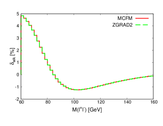
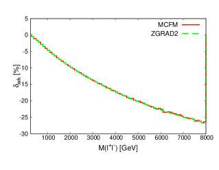
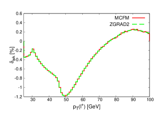
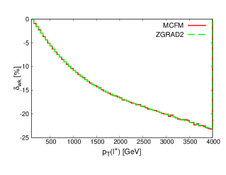
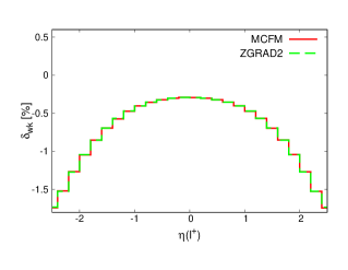
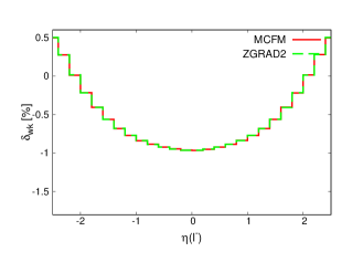
Figure 14: Comparison of MCFM (red, solid) and ZGRAD2 (green, dashed) predictions for the weak one-loop relative correction $\delta_{{\mathrm{wk}}}$ to the invariant mass of the lepton-pair ($M(l^{+}l^{-})$, top), lepton transverse momentum ($p_{T}(l^{+})$, middle), and lepton rapidities ($\eta(l^{\pm})$, bottom) distributions in NC DY production at the 13 TeV LHC. The correction is expressed as a percentage of the LO result in each bin, according to Eq. (35).

At ${\cal O}(\alpha^{2})$ the NC DY process also receives a contribution from the tree-level photon-induced process, $\gamma\gamma\to l^{+}l^{-}$. In Table 5 we compare the MCFM result and the results presented by Dittmaier and Huber in Ref. Dittmaier and Huber (2010) (denoted as DH in the following) for the total tree-level cross sections for the $q\bar{q}$- ($\sigma_{0}^{MCFM},\sigma_{0}^{DH}\left|\right._{FS/PS}$) and $\gamma\gamma$-initiated ($\sigma_{\gamma\gamma,0}^{MCFM}$) processes for various $M(l^{+}l^{-})$ regions at the 14 TeV LHC. The DH LO cross section $\sigma_{0}^{DH}\left|\right._{FS/PS}$ is obtained in the so-called Factorized Scheme (FS) or Pole Scheme (PS), which differ from the Complex-Mass Scheme (CMS) in the treatment of the $Z$ resonance (see Ref. Dittmaier and Huber (2010) for details). For the comparison we adopt the setup of Ref. Dittmaier and Huber (2010) and use the MRST2004QED Martin et al. (2005) PDF set. Note that the MRST2004QED PDF set is by now outdated and up-to-date PDF sets, such as NNPDF3.0QED Ball et al. (2013, 2015), and CT14QED Schmidt et al. (2016), should be used. In Table 5 we also compare the contribution of the LO photon-induced process relative to the ${\mathrm{q\bar{q}}}$-initiated process, $\delta_{\gamma\gamma,0}=\sigma_{\gamma\gamma,0}/\sigma_{0}$. We find that the LO cross sections $\sigma_{0}^{DH}$ and $\sigma_{0}^{MCFM}$ agree at the 0.15% level (and better for small $M(l^{+}l^{-})$), and that there is excellent agreement in $\delta_{\gamma\gamma,0}$. Note that in Ref. Dittmaier and Huber (2010) also the EW ${\cal O}(\alpha)$ corrections to $\gamma\gamma\to l^{+}l^{-}$ have been calculated and found to be negligible.

In Fig 15 we show MCFM predictions for the $M(l^{+}l^{-})$ distribution ($l=e$ or $\mu$) for the photon-induced tree-level production process at the 13 TeV LHC when using a variety of photon PDFs, compared to the $q\bar{q}$-induced NC DY distribution at LO (the setup of Table 4 is used with $\mu_{F}=\mu_{R}=M_{Z}$). The spread of predictions, especially at high invariant masses, indicates the large uncertainties associated with the photon PDF of current global PDF sets (see Refs. Ball et al. (2013, 2015); Schmidt et al. (2016) for a detailed discussion). Dedicated efforts to improve the knowledge of the photon PDF are under way Martin and Ryskin (2014); Harland-Lang et al. (2016); Manohar et al. (2016). In view of the situation presented in Fig. 15, we cannot conclusively assess by how much the positive photon-induced contribution affects the impact of the negative weak one-loop corrections on NC DY observables until these more precise determinations of photon PDFs become readily available.

$M(l^{+}l^{-})$ [GeV]	50-$\infty$	100-$\infty$	200-$\infty$	500-$\infty$	1000 -$\infty$	2000-$\infty$
$\sigma_{\gamma\gamma,0}^{MCFM}$ [fb]	1287.98(7)	377.77(5)	63.88(1)	3.9809(7)	0.35407(7)	0.018759(4)
$\sigma_{0}^{DH}\left|\right._{FS/PS}$ [fb]	738773(6)	32726.8(3)	1484.92(1)	80.9489(6)	6.80008(3)	0.303767(1)
$\sigma_{0}^{MCFM}$ [fb]	739272(13)	32881.5(6)	1484.37(30)	81.0745(16)	6.8103(1)	0.304209(5)
$\delta_{\gamma\gamma,0}^{DH}$[%]	0.17	1.15	4.30	4.92	5.21	6.17
$\delta_{\gamma\gamma,0}^{MCFM}$[%]	0.17	1.15	4.30	4.91	5.20	6.17

Table 5: MCFM cross sections for the tree-level photon-induced process, $\sigma_{\gamma\gamma,0}^{MCFM}$, for various ranges of the invariant di-lepton mass ($M(l^{+}l^{-})$) obtained with MRST2004QED at the 14 TeV LHC. We also show a comparison of the LO $q\bar{q}$-initiated NC DY cross section, $\sigma_{0}$, and of the ratio $\delta_{\gamma\gamma,0}=\sigma_{\gamma\gamma,0}/\sigma_{0}$ from MCFM and Table 1 of Ref. Dittmaier and Huber (2010) (labeled as DH).

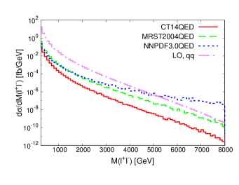
Figure 15: LO predictions for the invariant lepton-pair mass distribution for the photon-induced process and the $q\bar{q}$-initiated (pink, long-dashed-dotted) NC DY process at the 13 TeV LHC. The photon-induced LO prediction is obtained with different photon PDFs as provided by CT14QED (red, solid), MRST2004QED (green, dashed), and NNPDF3.0QED (blue, dotted).

III.2 Top-quark pair production

We perform a tuned comparison of our MCFM implementation of weak one-loop corrections to $t\bar{t}$ production at the LHC as presented in Section II.1.2 with the one presented by Kühn, Scharf and Uwer in Ref. Kühn et al. (2015) (denoted as KSU in the following). We adopt the setup used therein, which corresponds to the masses and couplings shown in Table 6. Furthermore, we set the renormalization and factorization scales equal to the mass of the top quark, $\mu_{F}=\mu_{R}=m_{t}$ and we employ the MSTW2008NNLO PDF set Martin et al. (2009) that specifies $\alpha_{s}(m_{Z})=0.11707$. With this setup the value of the strong coupling used in the calculation is $\alpha_{s}(m_{t})$, as given in the table.

$M_{W}=80.385\,\mathrm{GeV}$	$M_{Z}=91.1876\,\mathrm{GeV}$
$M_{H}=126\,\mathrm{GeV}$	$m_{t}=173.2\,\mathrm{GeV}$
$m_{b}=4.82\,\mathrm{GeV}$	$\alpha(m_{t})=1/127$
$\sin^{2}\theta_{W}=1-M_{W}^{2}/M_{Z}^{2}$	$\alpha_{s}(m_{t})=0.106823$

Table 6: Input parameters used in the validation of the weak one-loop corrections to the $t\bar{t}$ production process. These parameters are chosen in order to facilitate a comparison with the results of Ref. Kühn et al. (2015).

In Fig. 16 we present a comparison of the relative corrections to the parton-level processes, $u\bar{u}\to t\bar{t}$ and $gg\to t\bar{t}$ . In the case of the ${\mathrm{q\bar{q}}}$-initiated process we show results for $\delta_{{\mathrm{wk}}}$ of Eq. (35) separately for the weak one-loop vertex corrections (diagrams shown in the upper part of Fig. 6) and for the full ${\cal O}(\alpha_{s}^{2}\alpha)$ contribution (which now also includes the box diagrams in Fig. 6 and the virtual and real contributions of Fig. 8 and Fig. 9, respectively). The parton-level results presented in Fig. 8 of Ref. Kühn et al. (2015) only include weak one-loop vertex corrections, since the remaining ${\cal O}(\alpha_{s}^{2}\alpha)$ contributions were studied in detail and found to be very small. This is also supported by the results of our calculation shown in Fig. 16. Moreover, we observe that the agreement between the results of MCFM and those of KSU is excellent.

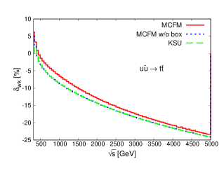
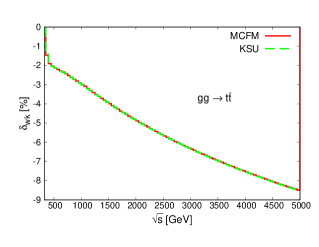
Figure 16: Comparison of relative corrections $\delta_{{\mathrm{wk}}}$ to the parton-level cross sections for $u\bar{u}\to t\bar{t}$ (left) and $gg\to t\bar{t}$ (right) from MCFM and the results from Fig. 8 of Ref. Kühn et al. (2015) (KSU) (green, dashed). The correction is expressed as a percentage of the LO ${\cal O}(\alpha_{s}^{2})$ cross section according to Eq. (35). In case of the $u\bar{u}\to t\bar{t}$ process the KSU results shown here only include weak one-loop vertex corrections, while MCFM results are provided for both the weak one-loop vertex corrections (blue, dotted) and the full ${\cal O}(\alpha_{s}^{2}\alpha)$ contribution (red, solid).

At the hadron level we perform the comparison for the LHC operating at 13 TeV, with no cuts applied to the top quarks except where noted specifically below. Note that the hadron-level results of Ref. Kühn et al. (2015) now also include the full ${\cal O}(\alpha_{s}^{2}\alpha)$ contributions, i.e. also including box diagrams and real corrections. For this set-up we find a LO cross section for ${\mathrm{t\bar{t}}}$ production at ${\cal O}(\alpha_{s}^{2})$ of,

$$\sigma_{\mathrm{LO}}=474.60(4)~{}\mathrm{pb}.$$ (39)

The overall effect of the full ${\cal O}(\alpha_{s}^{2}\alpha)$ contribution on the total cross section is rather small and results in a relative correction,

$$\delta_{{\mathrm{wk}}}=\frac{-9.509(1)~{}\mathrm{pb}}{474.60(4)~{}\mathrm{pb}}=-2.00\%.$$ (40)

This is in perfect agreement with the results from Ref. Kühn et al. (2015), which gives $\delta_{{\mathrm{wk}}}=-2.00$%.

We now turn to the comparison of results for differential distributions, in particular for the top-pair invariant mass distribution ($M(t\bar{t})$), the transverse momentum of the top quark ($p_{T}(t)$) and the rapidity difference between the top and anti-top quarks, $\Delta y(t\bar{t})=y(t)-y(\bar{t})$, where $y(t)$ and $y(\bar{t})$ are the rapidities in the lab frame. This comparison is presented in Fig. 17 where, for the $\Delta y(t\bar{t})$ distribution, a cut $M(t\bar{t})>2$ TeV has been applied. The KSU results are taken from Figs. 20 and 22 (right) of Ref. Kühn et al. (2015). While the parton-level results are in excellent agreement, we observe a small difference in the $M(t\bar{t})$ distribution at the 0.5% level at $M(t\bar{t})\approx 5$ TeV. We have not been able to trace the origin of this discrepancy, which may simply be due to the fact that different approaches for the treatment of IR singularities have been used, namely dipole subtraction and phase-space slicing. Each of these methods has its own challenges in obtaining precise numerical results at such large invariant masses.

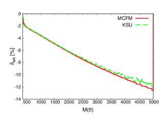
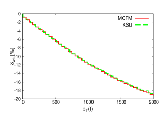
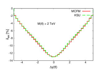
Figure 17: Comparison of relative corrections $\delta_{{\mathrm{wk}}}$ from MCFM (red, solid) and the results from Fig. 20 and Fig. 22 of Ref. Kühn et al. (2015) (KSU) (green, dashed) to the invariant mass distribution of the top-antitop pair ($M(t{\bar{t}})$) (top center), the transverse momentum of the top quark ($p_{T}(t)$) (left), and the rapidity difference between the top and anti-top quark ($\Delta y(t\bar{t})$) (right), in ${\mathrm{t\bar{t}}}$ production at the 13 TeV LHC. In the calculation of the $\Delta y(t\bar{t})$ distribution a cut of $M(t{\bar{t}})>2$ TeV is applied. The correction is expressed as a percentage of the LO ${\cal O}(\alpha_{s}^{2})$ cross section according to Eq. (35).

III.3 Di-jet production

We perform a tuned comparison of our MCFM implementation of di-jet production at ${\cal O}(\alpha_{s}^{2}\alpha)$ as described in Section II.1.3 with the results of Dittmaier, Huss, and Speckner in Ref. Dittmaier et al. (2012) (denoted as DHS in the following), and thus adopt the setup used therein, which corresponds to the masses and couplings shown in Table 4. The factorization scale ($\mu_{F}$) and renormalization scale ($\mu_{R}$) are set equal, $\mu_{F}=\mu_{R}=k_{T}(j_{1})$, where $k_{T}(j_{1})$ is the transverse momentum of the leading jet. The CTEQ6L1 set of PDFs Pumplin et al. (2002) is used, which corresponds to a strong coupling of $\alpha_{s}(M_{Z})=0.129783$. To identify the jets the anti-$k_{T}$ jet clustering algorithm is used with a pseudo-cone size of $R=0.6$, and the following jet cuts are applied:

$$k_{T}(j)>25\;\mathrm{GeV},\;\;\;|y(j)|<2.5.$$ (41)

A comparison of MCFM and DHS results for relative corrections in various ranges of the invariant mass of the two leading jets ($M(j_{1}j_{2})$) at the 14 TeV LHC is shown in Table 7. A similar comparison, for various ranges of the transverse momentum of the leading jet ($k_{T}(j_{1})$), is given in Table 8. In both cases we compare the relative one-loop weak corrections ($\delta_{{\mathrm{wk}}}$ of Eq. (35)) and the effect of additional tree-level contributions mediated by EW interactions ($\delta_{\mathrm{EW}}^{\mathrm{tree}}$). The latter correction is defined by,

$$\delta_{\mathrm{EW}}^{\mathrm{tree}}=\frac{d\sigma_{LO+ew}-d\sigma_{LO}}{d\sigma_{LO}}$$ (42)

where $\sigma_{LO}$ represents the QCD-mediated LO cross section of ${\cal O}(\alpha_{s}^{2})$, while $\sigma_{LO+ew}$ also contains the additional ${\cal O}(\alpha_{s}\alpha)$ and ${\cal O}(\alpha^{2})$ contributions due to the $Z,\gamma$ and $W$-exchange diagrams shown in Fig. 10. As can be seen from the tables, the inclusion of these terms partially cancels the effect of the weak one-loop corrections.

$M(j_{1}j_{2})$ [GeV]		$50-\infty$	$100-\infty$	$200-\infty$	$500-\infty$	$1000-\infty$	$2000-\infty$	$5000-\infty$
$\delta_{\mathrm{wk}}[\%]$	DHS	-0.02	-0.03	-0.07	-0.31	-0.88	-2.20	-5.53
	MCFM	-0.02	-0.03	-0.07	-0.31	-0.88	-2.23	-5.57
$\delta^{\mathrm{tree}}_{\mathrm{EW}}[\%]$	DHS	0.03	0.01	0.02	0.10	0.34	1.00	2.56
	MCFM	0.03	0.01	0.02	0.08	0.30	0.96	2.61

Table 7: Comparison of relative corrections $\delta_{\mathrm{wk}}$ of Eq. (35) and $\delta_{\mathrm{EW}}^{\mathrm{tree}}$ of Eq. (42) from MCFM and Table 1 of Ref. Dittmaier et al. (2012) (DHS) for various ranges of the invariant di-jet mass ($M(j_{1}j_{2})$) in di-jet production at the 14 TeV LHC.

$k_{T}(j_{1})$ [GeV]		$25-\infty$	$50-\infty$	$100-\infty$	$200-\infty$	$500-\infty$	$1000-\infty$	$2500-\infty$
$\delta_{\mathrm{wk}}[\%]$	DHS	-0.02	-0.08	-0.28	-0.84	-2.72	-5.48	-10.49
	MCFM	-0.02	-0.08	-0.28	-0.83	-2.75	-5.64	-10.41
$\delta^{\mathrm{tree}}_{\mathrm{EW}}[\%]$	DHS	0.03	0.03	0.12	0.36	1.44	4.62	18.28
	MCFM	0.03	0.03	0.11	0.33	1.42	4.72	18.88

Table 8: Comparison of relative corrections $\delta_{\mathrm{wk}}$ of Eq. (35) and $\delta_{\mathrm{EW}}^{\mathrm{tree}}$ of Eq. (42) from MCFM and Table 2 of Ref. Dittmaier et al. (2012) (DHS) for various ranges of the transverse momentum of the leading jet ($k_{T}(j_{1})$) in di-jet production at the 14 TeV LHC.

A comparison of the relative corrections to the di-jet invariant mass ($M(j_{1}j_{2})$) and the transverse jet momentum distributions of the leading jet ($k_{T}(j_{1})$) at the 14 TeV LHC is shown in Fig. 18. As can been seen, all of the MCFM results for di-jet production at the LHC are in good agreement with those presented by DHS in Ref. Dittmaier et al. (2012), with only small differences at large values of $k_{T}(j_{1})$ of at most $3\%$ of the relative correction.

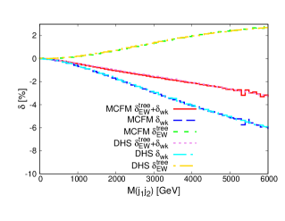
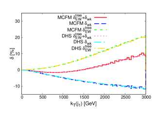
Figure 18: Comparison of relative corrections $\delta_{{\mathrm{wk}}}$ of Eq. (35) (blue, dashed and light blue, long-dashed-dotted), $\delta_{\mathrm{EW}}^{\mathrm{tree}}$ of Eq. (42) (green, short-dashed and yellow, dotted-long-dashed), and their sum (red, solid and pink, dotted) from MCFM and the results of Figures 9 and 12 of Ref. Dittmaier et al. (2012) (DHS). Results are shown for the invariant di-jet mass ($M(j_{1}j_{2})$) (left)) and transverse jet momentum distributions for the leading jet ($k_{T}(j_{1})$) (right) in di-jet production at the 14 TeV LHC.

IV Effectiveness of the Sudakov approximation

Using the two implementations of weak one-loop corrections in MCFM, i. e. the full corrections and their Sudakov approximation as described in Section II.2, we can now easily assess the effectiveness of the Sudakov approximation of Ref. Denner and Pozzorini (2001b) in the tails of kinematic distributions by comparing with the exact results. As pointed out earlier Moretti et al. (2006a); Kühn et al. (2015), the Sudakov approximation is expected to have only limited application in ${\mathrm{t\bar{t}}}$ and di-jet production. The Sudakov logarithms are only dominant when all invariants are much larger than the weak gauge boson mass and, in general, these terms fail to capture the correct angular distribution of particles in the final state. Nevertheless, a comparison of the exact and Sudakov results may serve as a guide for cases in which a full, exact calculation is infeasible and the Sudakov approximation is the only available recourse.

If not mentioned otherwise, all results in this section are obtained with MCFM using the setup and cuts described in Section III. For the sake of definiteness, we define a relative weak Sudakov correction in direct analogy to Eq. (35) through,

$$\delta_{{\mathrm{Sudakov}}}=\frac{d\sigma_{NLO}^{{\mathrm{Sudakov}}}-d\sigma_{LO}}{d\sigma_{LO}},$$ (43)

where $\sigma_{NLO}^{{\mathrm{Sudakov}}}$ includes the NLO Sudakov corrections described in Section II.2.

IV.1 Neutral-Current Drell-Yan process

As we have seen in Section III.1 the effect of the weak one-loop corrections on the total rate for the NC DY process is rather small. However the situation is quite different when investigating the effect on kinematic distributions such as the invariant mass of the lepton pair and the transverse momentum of the leptons. These are shown for both the exact weak corrections $\delta_{{\mathrm{wk}}}$ and the Sudakov approximation $\delta_{{\mathrm{Sudakov}}}$, over ranges extending to multi-TeV values, in Fig. 19. We have used the same setup and cuts described in Section III.1 apart from increasing the cut on $M(l^{+}l^{-})$ to 200 GeV. The Sudakov approximation shows good agreement with the exact NLO calculation in the $p_{T}(l^{+})$ distribution but there is a discrepancy in the $M(l^{+}l^{-})$ distribution at the level of about $3\%$ for $M(l^{+}l^{-})\sim 8$ TeV.

Figure 19: Relative weak one-loop corrections from MCFM to the invariant lepton-pair mass ($M(l^{+}l^{-}$, $l=e,\mu)$) (left) and lepton transverse momentum ($p_{T}(l^{+})$) (right) distributions in the NC DY process at the 13 TeV LHC. The correction is expressed as a percentage of the LO result and results are shown for both the exact ($\delta_{{\mathrm{wk}}}$ of Eq. (35)) (red, solid) and approximate Sudakov ($\delta_{{\mathrm{Sudakov}}}$ of Eq. (43)) calculation, the latter with (blue, dotted) and without (pink, long-dashed-dotted) the $\gamma-Z$ box contribution of Eq. (IV.1).

We can trace this remaining difference to the contribution of the $\gamma-Z$ box in the Sudakov approximation, which is not included in the exact weak one-loop correction, since it is considered part of the QED ${\cal O}(\alpha)$ correction to the NC DY process. To illustrate the impact of the $\gamma-Z$ box we evaluate the contribution of this diagram to the matrix element squared at ${\cal O}(\alpha^{3})$ in the leading approximation (LA) at high energies. We can then identify the part proportional to $\log\left(\hat{t}/\hat{u}\right)\log\left(\hat{s}/M_{Z}^{2}\right)$ as the contribution of the $\gamma-Z$ box to the Sudakov approximation of Eq. (24), which reads:

$$\overline{\sum}\mathrm{Re}\left(\delta^{\mathrm{SSC,Z}}\mathcal{M}_{0}\times\mathcal{M}_{0}^{*}\right) =\frac{2}{3}\alpha^{3}\pi\cdot\frac{-16}{\hat{s}^{2}}\cdot\log\left(\frac{\hat{t}}{\hat{u}}\right)\log\left(\frac{\hat{s}}{M_{Z}^{2}}\right)\cdot\Bigg{\{}$$

$$+Q_{q}^{2}Q_{l}^{2}\left[g_{v}^{q}g_{v}^{l}\left(\hat{t}^{2}+\hat{u}^{2}\right)-g_{a}^{q}g_{a}^{l}\left(\hat{t}^{2}-\hat{u}^{2}\right)\right]$$

$$+2~{}Q_{q}Q_{l}\left[\left({g_{v}^{q}}^{2}+{g_{a}^{q}}^{2}\right)\left({g_{v}^{l}}^{2}+{g_{a}^{l}}^{2}\right)\left(\hat{t}^{2}+\hat{u}^{2}\right)-4g_{v}^{q}g_{v}^{q}g_{a}^{q}g_{a}^{l}\left(\hat{t}^{2}-\hat{u}^{2}\right)\right]$$

$$+(g_{v}^{q}g_{v}^{l}+g_{a}^{q}g_{a}^{l})\left[\left(g_{v}^{q}g_{v}^{l}+g_{a}^{q}g_{a}^{l}\right)^{2}+3\left(g_{v}^{q}g_{a}^{l}+g_{a}^{q}g_{v}^{l}\right)^{2}\right]\hat{u}^{2}$$

$$-(g_{v}^{q}g_{v}^{l}-g_{a}^{q}g_{a}^{l})\left[\left(g_{v}^{q}g_{v}^{l}-g_{a}^{q}g_{a}^{l}\right)^{2}+3\left(g_{v}^{q}g_{a}^{l}-g_{a}^{q}g_{v}^{l}\right)^{2}\right]\hat{t}^{2}\Bigg{\}}$$ (44)

In Fig. 19 we also show the effect of subtracting this contribution from the Sudakov approximation of Eq. (24). As expected, this modified Sudakov approximation now represents an excellent description of the full one-loop weak correction to the lepton-pair invariant mass distribution.

In Fig. 20, we compare the relative weak one-loop corrections $\delta_{{\mathrm{wk}}}$ and $\delta_{{\mathrm{Sudakov}}}$ to the pseudo-rapidity distribution of the charged leptons, where we apply successive cuts on the lepton-pair invariant mass at 2 TeV and 5 TeV in order to focus on the high-energy behavior. Despite this cut, the exact and Sudakov calculations are not in good agreement outside the very central rapidity region unless the $\gamma-Z$ box contribution of Eq. (24) is subtracted from $\delta_{{\mathrm{Sudakov}}}$. When this is the case, this modified Sudakov approximation agrees well with the exact calculation at $M(l^{+}l^{-})>5$ TeV. However, overall the effect of the weak one-loop corrections on the lepton rapidity distributions is rather mild, since they are not very sensitive to the presence of the weak Sudakov logarithms.

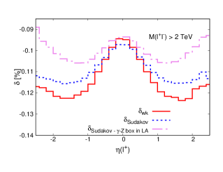
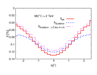
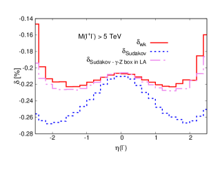
Figure 20: Relative weak one-loop corrections to the pseudorapidity distributions of the positively (left) and negatively (right) charged leptons in the NC DY process at the 13 TeV LHC. The correction is expressed as a percentage of the LO result and results are shown for both the exact ($\delta_{{\mathrm{wk}}}$ of Eq. (35)) (red, solid) and approximate Sudakov ($\delta_{{\mathrm{Sudakov}}}$ of Eq. (43)) calculation, the latter with (blue, dotted) and without (pink, long-dashed-dotted) the $\gamma-Z$ box contribution of Eq. (IV.1).

Another observable that is interesting to measure at the LHC is the forward-backward asymmetry of the charged leptons as a function of the invariant mass of the lepton pair, $A_{FB}(M(l^{+}l^{-}))$. It is defined by Baur et al. (1998),

$$A_{\rm FB}=\frac{F-B}{F+B}$$ (45)

where

$$F=\int_{0}^{1}\frac{{\rm d}\sigma}{{\rm d}\cos\theta^{*}}\,{\rm d}\cos\theta^{*},\qquad B=\int_{-1}^{0}\frac{{\rm d}\sigma}{{\rm d}\cos\theta^{*}}\,{\rm d}\cos\theta^{*}.$$ (46)

$\cos\theta^{*}$ is given in the Collins-Soper frame Collins and Soper (1977) by,

$$\cos\theta^{*}=\frac{|p_{z}(l^{+}l^{-})|}{p_{z}(l^{+}l^{-})}~{}\frac{2}{M(l^{+}l^{-})\sqrt{M^{2}(l^{+}l^{-})+p_{T}^{2}(l^{+}l^{-})}}\left[p^{+}(l^{-})p^{-}(l^{+})-p^{-}(l^{-})p^{+}(l^{+})\right]\;,$$ (47)

where,

$$p^{\pm}=\frac{1}{\sqrt{2}}\left(E\pm p_{z}\right),$$ (48)

and $E$, $p_{z}$ are the energy and longitudinal component of the momentum respectively.

This observable is sensitive to the weak mixing angle and, in the vicinity of the $Z$ resonance where the number of events is very high, precision measurements of this quantity have been made both at the Tevatron Aaltonen et al. (2016); Abazov et al. (2015) and the LHC Chatrchyan et al. (2011); Aad et al. (2015); Aaij et al. (2015). However, it is also interesting to study this observable far from the resonance region. For instance, in the high-invariant mass region $A_{FB}$ can be used in the search for extra gauge bosons ($Z^{\prime}$) (see, for example, Ref. Accomando et al. (2016)).

The impact of the exact weak one-loop corrections on $A_{FB}$, compared to the Sudakov approximation with and without the contribution from the $\gamma-Z$ box diagram of Eq. (IV.1), is shown in Fig. 21. We note that the effect of the weak corrections is well-described by the Sudakov approximation throughout the distribution. These effects are relatively mild for invariant masses that have been probed with good precision so far (around 1 TeV), but grow as large as $-12\%$ in the far tail.

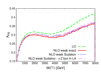
Figure 21: Differential lepton forward-backward asymmetry $A_{FB}$ with respect to the invariant mass of the charged lepton pair in the NC DY process at the 13 TeV LHC. Results are shown for the LO (green, dashed) prediction and for both the exact (red, solid) and approximate Sudakov calculation, the latter with (blue, dotted) and without (pink, long-dashed-dotted) the $\gamma-Z$ box contribution of Eq. (IV.1).

IV.2 Top-quark pair production

We now turn to the case of top-quark pair production, where we follow the setup already used in Section III.2. Figure 22 shows the results of the comparison in the cases of the $p_{T}(t)$ and $\Delta y(t\bar{t})$ distributions. For the distribution of the rapidity difference we have applied an additional ${\mathrm{t\bar{t}}}$ invariant mass cut of $M(t\bar{t})>2$ TeV. Agreement between the exact and approximate calculations is almost perfect for $p_{T}(t)$, but this is not the case for $\Delta y(t\bar{t})$. There the Sudakov approximation is only close to the exact result for small rapidity differences, $|\Delta y(t\bar{t})|<2$, due to angular dependence in the corrections that is not captured in the Sudakov approximation.

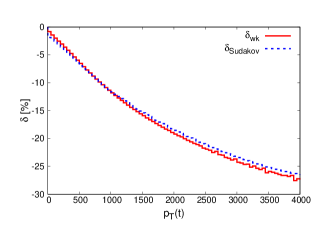
Figure 22: Relative weak corrections to the $p_{T}(t)$ (left) and $\Delta y(t\bar{t})$ (right) distributions in ${\mathrm{t\bar{t}}}$ production at the $13$ TeV LHC. The correction is expressed as a percentage of the LO result and is shown for the exact weak relative correction $\delta_{{\mathrm{wk}}}$ of Eq. (35) (red, solid) and the Sudakov approximation of $\delta_{{\mathrm{Sudakov}}}$ of Eq. (43) (blue, dotted).

The situation for the distribution of the invariant mass of the top pair is shown in Fig. 23. In this case the Sudakov approximation also does not describe the effect of the weak corrections on the $M(t{\bar{t}})$ distribution very well. Since Fig. 22 demonstrates that the approximation works best for more central rapidities, we repeat the comparison of the $M(t{\bar{t}})$ distribution after application of rapidity cuts on the top and anti-top quarks. We consider both central production of top quarks, $|y(t,\bar{t})|<1$ and an intermediate case, $|y(t,\bar{t})|<2.5$. Agreement is substantially improved after the application of a moderate rapidity cut on the top quarks, while for highly-central top quarks the approximation describes the exact result extremely well over the entire range.

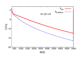
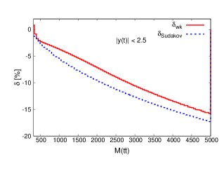
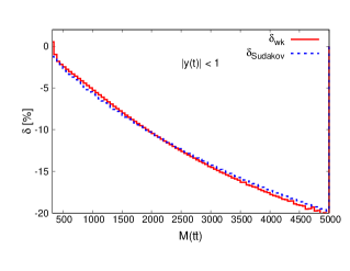
Figure 23: Relative weak corrections to $M(t{\bar{t}})$ in ${\mathrm{t\bar{t}}}$ production at the $13$ TeV LHC with no cuts applied (top left), after application of a moderate rapidity cut (top right) and for central top quarks (center). The correction is expressed as a percentage of the LO result and is shown for the exact weak relative correction $\delta_{{\mathrm{wk}}}$ of Eq. (35) (red, solid) and the Sudakov approximation $\delta_{{\mathrm{Sudakov}}}$ of Eq. (43) (blue, dotted).

IV.3 Di-jet Production

Here we compare the exact calculation of di-jet production at ${\cal O}(\alpha_{s}^{2}\alpha)$ described in Section II.1.3 with the Sudakov approximation described in Section II.2.3. In Fig. 24 we show the comparison for the di-jet invariant mass ($M(j_{1}j_{2})$), the transverse momenta of the leading and next-to-leading (in $k_{T}$) jets, and the absolute rapidity difference between these two jets ($\Delta y(j_{1}j_{2})$). Results are shown for the relative corrections for the 13 TeV LHC in the setup used in Section III.3. For the distribution of the rapidity difference we have applied an additional di-jet invariant mass cut of $M(j_{1}j_{2})>2$ TeV.

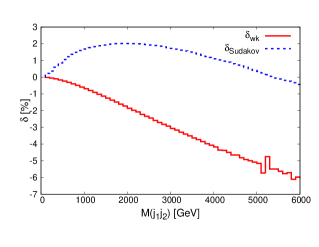
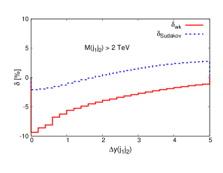
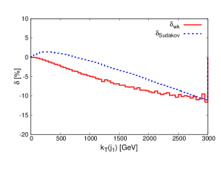
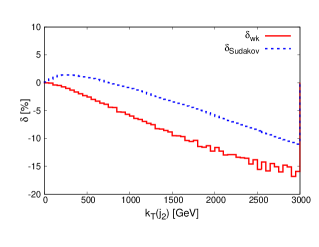
Figure 24: Relative weak corrections to the invariant mass (upper left), the absolute rapidity difference between the two leading jets (upper right), and the transverse momentum distributions of leading (lower left) and subleading (lower right) jets in di-jet production at the 13 TeV LHC. The correction is expressed as a percentage of the LO ${\cal O}(\alpha_{s}^{2})$ cross section and is shown for the exact weak relative corrections of Eq. (35) (red, solid) and the Sudakov approximation of Eq. (43) (blue, dotted).

We observe that the Sudakov approximation has little utility in this case, with substantial differences from the exact calculation in each distribution. This can be traced to the rich angular structure of the weak corrections, especially in the four-quark subprocesses, whose admixture is impossible to capture in an approximate form of Sudakov-type. For example, the QCD virtual corrections to the four-quark amplitude shown in Figs. 11, 12 (and the corresponding real corrections), which also contribute at ${\cal O}(\alpha_{s}^{2}\alpha)$, are not captured by the Sudakov approximation, but still have a sizeable impact on the distributions shown here. This is also highlighted by the fact that, in contrast to the case of top-quark pair production, there is no region in $\Delta y(t\bar{t})$ in Fig. 24 where the results of the exact weak and approximate calculations are close, so that the application of a central rapidity cut does little to improve the effectiveness of the Sudakov approximation.

V Combination of QCD and Weak Corrections

In this section we will consider the combination of the exact NLO weak corrections that we have presented, with QCD corrections at NLO and beyond. The aim of this section is to compare the sizes of the two effects and to demonstrate the inherent ambiguity in how the two should be combined, particularly in cases where either correction, or both, is large.

To illustrate this we will consider two procedures for combining the corrections. One straightforward method is to simply add the weak corrections, $\sigma_{{\mathrm{wk}}}$ to the NLO or NNLO QCD cross section,

$$\sigma_{QCD+{\mathrm{wk}}}=\sigma_{(N)NLO\,QCD}+\sigma_{{\mathrm{wk}}}\;,$$ (49)

An alternative is to combine them using a “multiplicative” procedure,

$$\sigma_{QCD\times{\mathrm{wk}}}=\sigma_{(N)NLO\,QCD}\left(1+\frac{\sigma_{{\mathrm{wk}}}}{\sigma_{LO}}\right)\;.$$ (50)

This procedure should better account for factorizable higher-order mixed QCD-weak corrections. Compared to the additive procedure, this approach enhances the impact of weak corrections in regions where the QCD corrections are large. To illustrate the numerical impact of these two approaches we discuss in the following the relative corrections with respect to the (N)NLO QCD cross section defined as,

$$\delta_{{\mathrm{add}}}=\frac{\sigma_{QCD+{\mathrm{wk}}}-\sigma_{(N)NLO\,QCD}}{\sigma_{(N)NLO\,QCD}}=\frac{\sigma_{{\mathrm{wk}}}}{\sigma_{(N)NLO\,QCD}}\;$$ (51)

for the additive approach, and

$$\delta_{{\mathrm{prod}}}=\frac{\sigma_{QCD\times{\mathrm{wk}}}-\sigma_{(N)NLO\,QCD}}{\sigma_{(N)NLO\,QCD}}=\frac{\sigma_{{\mathrm{wk}}}}{\sigma_{LO}}$$ (52)

for the “multiplicative” procedure. Similar studies of different combinations of QCD and EW corrections can also be found for instance in Ref. Kühn et al. (2015) for ${\mathrm{t\bar{t}}}$ production and in Refs. Li and Petriello (2012); Dittmaier et al. (2012); Mishra et al. (2013); Alioli et al. (2016) for NC DY production. In case of DY processes, the mixed QCD-electroweak corrections at ${\cal O}(\alpha_{s}\alpha)$ have been calculated in the pole approximation in Refs. Dittmaier et al. (2014, 2016), which considerably improves predictions in the resonance region.

V.1 NNLO QCD and Weak Corrections to the NC Drell-Yan process

The NNLO QCD corrections to the Drell-Yan process can be computed in MCFM Boughezal et al. (2016) and their combination with the weak corrections is therefore particularly straightforward. For the results presented here we retain the parameters and setup of the previous sections, with the exception that all computations are now performed with the NNLO MSTW2008 set.

Our results are shown in Figure 25. As is well-known, the effect of NNLO QCD corrections, relative to LO, is large and positive throughout the distribution. This is apparent from the left-hand plot. The right-hand plot compares the two combination procedures by plotting the relative corrections with respect to the NNLO QCD result, $\delta_{{\mathrm{add}}}$ and $\delta_{{\mathrm{prod}}}$ as defined in Eqs. (49) and (50), respectively. Since these are normalized to the NNLO QCD prediction, the result for $\delta_{{\mathrm{prod}}}$ could have been read-off directly from Figure 19 (c.f. Eq. (52)). The fact that both corrections are substantial means that the two procedures give noticeably different results for $M(l^{+}l^{-})>2$ TeV. As a point of reference, in this plot we also show the theoretical uncertainty resulting from the choice of scale in the NNLO QCD calculation. This is obtained by considering the envelope of predictions obtained when using alternative scales given by,

$$(\mu_{F}/M_{Z},\mu_{R}/M_{Z})=\left\{(0.5,0.5),~{}(2,2),~{}(0.5,1),~{}(0.5,2),~{}(1,0.5),~{}(2,0.5)\right\}\;.$$ (53)

With this prescription the scale uncertainty is as large as $5$% in the tail of the distribution, but is still smaller than the effect of combining with weak corrections using either procedure. It is therefore clear that both effects must be included, with an accompanying uncertainty associated with the choice of combination procedure, in order to provide the best theoretical prediction. As a conservative estimate of the combination uncertainty one might simply take the difference between the two procedures, which is of the same order as the QCD scale uncertainty.

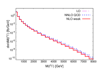
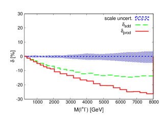
Figure 25: Left: comparison of the effect of NLO weak (red, solid) and NNLO QCD corrections (blue, dotted) on the invariant mass distribution of the di-lepton pair in the NC DY process at 13 TeV. The LO distribution is also shown (pink, long-dashed-dotted). Right: a comparison of the two procedures ($\delta_{{\mathrm{add}}}$ of Eq. (51) (green, dashed) and $\delta_{{\mathrm{prod}}}$ of Eq. (52) (red, solid)) used to combine NNLO QCD and NLO weak effects, together with the scale uncertainty in the pure NNLO QCD calculation (blue band). The NNLO QCD results have been obtained with MCFM Boughezal et al. (2016).

V.2 NNLO QCD and Weak One-loop Corrections to Top-Quark Pair Production

We now consider the combination of corrections to the top-quark pair process, namely exact NLO weak corrections with QCD corrections at NNLO. Since these corrections are not yet available in differential form in a public code, we will compare our NLO weak results with the NNLO results that have been published so far Czakon et al. (2016a, b).

We first focus on results for the Tevatron collider, where the NNLO results are easily read-off from tables presented in Ref. Czakon et al. (2016b). In order to match the results of that study we modify our input parameters from the previous sections slightly, to those shown in Table 9. As before, we use $\mu_{F}=\mu_{R}=m_{t}$ and we employ the NNLO MSTW2008 PDF set Martin et al. (2009). Note that, in order to validate our setup, we have recomputed the predictions at LO and NLO QCD using MCFM and found perfect agreement.

$M_{W}=80.398\,\mathrm{GeV}$	$M_{Z}=91.1876\,\mathrm{GeV}$
$M_{H}=126\,\mathrm{GeV}$	$m_{t}=173.3\,\mathrm{GeV}$
$m_{b}=4.82\,\mathrm{GeV}$	$\alpha(m_{t})=1/132.3407$
$\sin^{2}\theta_{W}=1-M_{W}^{2}/M_{Z}^{2}$	$\alpha_{s}(m_{t})=0.125666$

Table 9: Input parameters used for the calculation of the NLO weak corrections in the setup used to calculate the NNLO QCD corrections to top-quark pair production at the Tevatron in Ref. Czakon et al. (2016b).

Our results are presented in the form of per-bin corrections to a selection of observables, following the original presentation of NNLO QCD results in Ref. Czakon et al. (2016b). Results are shown for $M(t\bar{t})$ (Table 10) and $p_{T}(t)$ (Table 11). We first note that the effect of the NNLO QCD corrections is typically very small, at the level of a few percent of the NLO QCD result, but is as large as almost $20\%$ for the highest $M(t\bar{t})$ bin. As expected, the effect of the NLO weak corrections is readily apparent in the $M(t\bar{t})$ and $p_{T}(t)$ distributions. The onset of the Sudakov logarithms is clear in the $M(t\bar{t})$ results, although the weak corrections are non-negligible (and positive) in the first bin. The NLO weak effects are of a similar size to the corrections from NNLO QCD and the two clearly must be taken into account together. This is even more clear in the $p_{T}(t)$ distribution, where the effects of the NLO weak corrections are larger than those due to NNLO QCD for $p_{T}(t)>200$ GeV.

$M(t\bar{t})$ [GeV]	$d\sigma/dM(t\bar{t})$ [pb/bin]
	NLO QCD	NNLO QCD corr	NLO weak corr
[240 ; 412.5]	$2.96~{}\times~{}10^{0}$	$0.17~{}\times~{}10^{0}$	$0.05~{}\times~{}10^{0}$
[412.5 ; 505]	$2.47~{}\times~{}10^{0}$	$0.12~{}\times~{}10^{0}$	$-0.01~{}\times~{}10^{0}$
[ 505 ; 615 ]	$9.20~{}\times~{}10^{-1}$	$0.30~{}\times~{}10^{-1}$	$-0.15~{}\times~{}10^{-1}$
[ 615 ; 750 ]	$2.66~{}\times~{}10^{-1}$	$0.07~{}\times~{}10^{-1}$	$-0.08~{}\times~{}10^{-1}$
[750 ; 1200]	$6.20~{}\times~{}10^{-2}$	$0.16~{}\times~{}10^{-2}$	$-0.27~{}\times~{}10^{-2}$
[ 1200 ; $\infty$]	$1.07~{}\times~{}10^{-4}$	$0.20~{}\times~{}10^{-4}$	$-0.10~{}\times~{}10^{-4}$

Table 10: The $M(t\bar{t})$ differential distribution in NLO QCD and the corrections due to NNLO QCD and NLO weak effects in ${\mathrm{t\bar{t}}}$ production at the Tevatron. The NLO and NNLO QCD results are taken from Ref. Czakon et al. (2016b).

$p_{T}(t)$ [GeV]	$d\sigma/dp_{T}(t)$ [pb/bin]
	NLO QCD	NNLO QCD corr	NLO weak corr
[ 0 ; 45 ]	$1.15~{}\times~{}10^{0}$	$0.08~{}\times~{}10^{0}$	$0.02~{}\times~{}10^{0}$
[ 45 ; 90 ]	$2.27~{}\times~{}10^{0}$	$0.12~{}\times~{}10^{0}$	$0.02~{}\times~{}10^{0}$
[ 90 ; 140]	$1.88~{}\times~{}10^{0}$	$0.09~{}\times~{}10^{0}$	$0.00~{}\times~{}10^{0}$
[140 ; 200]	$9.81~{}\times~{}10^{-1}$	$0.29~{}\times~{}10^{0}$	$-0.01~{}\times~{}10^{0}$
[200 ; 300]	$3.67~{}\times~{}10^{-1}$	$-0.02~{}\times~{}10^{-1}$	$-0.11~{}\times~{}10^{-1}$
[300 ; 500]	$4.20~{}\times~{}10^{-2}$	$-0.13~{}\times~{}10^{-2}$	$-0.24~{}\times~{}10^{-2}$
[500 ; $\infty$ ]	$2.21~{}\times~{}10^{-4}$	$0.04~{}\times~{}10^{-4}$	$-0.25~{}\times~{}10^{-4}$

Table 11: The $p_{T}(t)$ differential distribution in NLO QCD and the corrections due to NNLO QCD and NLO weak effects in ${\mathrm{t\bar{t}}}$ production at the Tevatron. The NLO and NNLO QCD results are taken from Ref. Czakon et al. (2016b).

In Ref. Czakon et al. (2016b) the NNLO QCD predictions have been compared with data from the DØ collaboration Abazov et al. (2014). We note that, although the size of the NLO weak corrections is comparable to the NNLO QCD ones in some of the bins, even the combined effects remain rather small. As a result, the inclusion of the NLO weak corrections does not significantly alter the extent of the agreement of the Standard Model prediction with the experimental data.

As we have already observed, the effects of the weak corrections should be larger at the LHC. The amount of data collected means that the ATLAS and CMS collaborations are sensitive to top quarks produced further above threshold, and the data is subject to significantly smaller experimental uncertainties. In order to combine our calculations with NNLO QCD corrections we use the predictions of Ref. Czakon et al. (2016a), which were compared with results from the CMS collaboration Khachatryan et al. (2015a). These results represent an analysis of the full $19.6$ fb^-1 data set taken at $8$ TeV. The distribution that is most sensitive to the weak corrections, and for which we can readily extract the effect of NNLO QCD, is the transverse momentum of the top quarks. For this analysis we do not distinguish between top and anti-top quarks, instead including both in the distribution, and normalize to the total cross-section. Our results are shown in Fig. 26. The NNLO QCD comparison was shown in Ref. Czakon et al. (2016a). Here we ameliorate that analysis by including also the NLO weak corrections, which are simply added on top of the NNLO predictions according to Eq. (49). We see that, although the shape of this distribution is slightly better described throughout, a difference in shape between the data and NNLO QCD+NLO weak theory remains. Since the effect of the weak corrections is rather small the alternative combination of Eq. (50) would yield almost identical results.

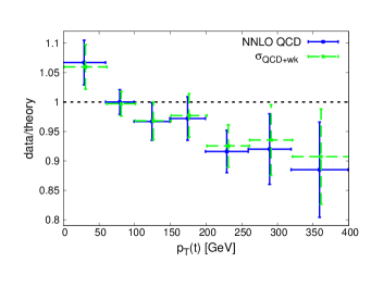
Figure 26: Comparison of NNLO QCD (blue, solid) and combined NNLO QCD+NLO weak (green, dashed) predictions for the $p_{T}(t)$ distribution in ${\mathrm{t\bar{t}}}$ production with 8 TeV CMS data Khachatryan et al. (2015a). The data is divided by the theoretical prediction in each bin of the top quark $p_{T}$. The NNLO QCD predictions are taken from Ref. Czakon et al. (2016a).

V.3 NLO QCD and Weak Corrections to Di-jet Production

Almost-complete results for di-jet production at hadron colliders have recently been presented through NNLO QCD Currie et al. (2014a, 2013, b); Pires (2015). However, here we restrict ourselves to the NLO QCD results that can be easily computed using the publicly available Monte-Carlo program MEKS Gao et al. (2013) (higher-order QCD corrections to di-jet production are not available in MCFM).

Figure 27 (left) shows the distribution of the invariant mass of the two leading jets at LO, at NLO QCD or after inclusion of NLO weak corrections. The NLO QCD corrections are rather mild at small invariant masses, but increase the cross-section by a factor of around $1.7$ in the multi-TeV range. This leads to a substantial difference between $\delta_{{\mathrm{add}}}$ and $\delta_{{\mathrm{prod}}}$ in the tail of the distribution, as shown in Fig. 27 (right). However the size of the combined correction, in either approach, is relatively small, for instance in comparison with the impact of the weak corrections in the NC DY case (Fig. 25).

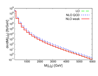
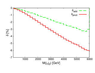
Figure 27: Left: comparison of the effect of NLO weak (red, solid) and NLO QCD (blue, dotted) corrections on the invariant mass distribution of the di-jet pair in di-jet production at the 13 TeV LHC. The LO QCD distribution at ${\cal O}(\alpha_{s}^{2})$ is also shown (green, dashed). Right: a comparison of the two procedures ($\delta_{{\mathrm{add}}}$ of Eq. (51) (green, dashed) and $\delta_{{\mathrm{prod}}}$ of Eq. (52) (red, solid)) used to combine NLO QCD and NLO weak effects. The NLO QCD results have been obtained with MEKS (version 1.0) Gao et al. (2013).

One of the interesting analyses of di-jet production at the LHC is the search for new physics beyond the Standard Model through a study of the scattering angle between the two jets. The production of jets through QCD is dominated by small-angle scattering, while additional interactions, for instance through a contact term Chiappetta and Perrottet (1991), lead to jet production at much wider angles Harris and Kousouris (2011). Both ATLAS Aad et al. (2016) and CMS Khachatryan et al. (2015b); The CMS Collaboration (2015) have taken advantage of this observation in order to place stringent constraints on various models of new physics.

Here we will consider the effect of weak corrections under a set of cuts used by a recent CMS analysis The CMS Collaboration (2015). The key observable, $\chi_{\mathrm{dijet}}$, is simply related both to the scattering angle and to the rapidity between the two leading jets ($y(j_{1},j_{2})$),

$$\chi_{\mathrm{dijet}}=\exp\left(|y(j_{1})-y(j_{2})|\right)\;.$$ (54)

We used the CT14 PDF set to produce the result in the same setup as used by CMS in Ref. The CMS Collaboration (2015). We use the anti-$k_{T}$ jet algorithm with $R=0.4$ and apply a cut $y_{\mathrm{boost}}=\frac{1}{2}|y(j_{1})+y(j_{2})|<2.22$. In Fig. 28 we show the normalized $\chi_{\mathrm{dijet}}$ distribution for a low and high invariant di-jet mass bin, also used in the CMS analysis, calculated at NLO QCD with MEKS (version 1.0) Gao et al. (2013) and when adding the MCFM prediction for the LO EW and ${\cal O}(\alpha_{s}^{2}\alpha)$ contribution. As expected, the weak one-loop corrections are most significant in the highest mass bin where the ${\cal O}(\alpha_{s}^{2}\alpha)$ contribution reduces the NLO QCD distribution by 9.8% at small values of $\chi_{\mathrm{dijet}}$. The LO EW contribution largely cancels the weak corrections so that the overall effect is an increase of the NLO QCD result by 2% in the first $\chi_{\mathrm{dijet}}$ bin. Our results are consistent with the findings presented in the CMS analysis The CMS Collaboration (2015), which is based on the calculation of Ref. Dittmaier et al. (2012). It is interesting to note that the new physics scenarios under consideration in Ref. The CMS Collaboration (2015) have their largest impact in the high-mass bin for small values of $\chi_{\mathrm{dijet}}$, i. e. exactly in the same kinematic regime where weak corrections become important.

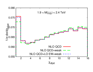
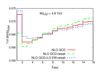
Figure 28: Normalized $\chi_{\mathrm{dijet}}$ distributions in di-jet production at the 13 TeV LHC in a low (left) and high (right) invariant di-jet mass bin at NLO QCD (red, solid) and when adding the ${\cal O}(\alpha_{s}^{2}\alpha)$ (green, dashed) and LO EW (blue, dotted) contributions. The NLO QCD results have been obtained with MEKS (version 1.0) Gao et al. (2013).

VI Conclusions

The role of electroweak corrections in the comparison of future LHC data with theoretical predictions in the Standard Model is becoming increasingly important. As the availability of higher-order perturbative QCD corrections extends past NLO, to NNLO and beyond, the resulting cross-sections often suffer from a residual theoretical uncertainty that is comparable in size to the expected size of electroweak corrections. Moreover, as the LHC collects more data it will begin to probe, with reasonable precision, final states with energies in the multi-TeV region. Such configurations receive one-loop electroweak corrections that are especially enhanced, by Sudakov logarithms of the form $\alpha\log^{2}\left(M_{\rm{final}}/M_{W}\right)$ with $M_{\rm final}$ being the invariant mass of the leading pair of final-state particles, so that including these effects is particularly important.

In this paper we have recomputed one-loop electroweak corrections at the LHC, to three processes of considerable importance: Neutral-Current Drell-Yan, top-quark pair and di-jet production. As well as performing exact calculations of these corrections, we have also considered the approximation obtained by retaining only leading and subleading Sudakov logarithms, following the approach of Refs. Denner and Pozzorini (2001a, b). We have also performed a detailed comparison of the efficacy of this approximation in order to glean insight into situations in which it is less effective or fails altogether. For the processes at hand, the Sudakov approximation is excellent for the case of NC DY, less accurate for top-quark pair production and poor for the di-jet process.

Our calculations have been implemented in the framework of the parton-level Monte Carlo code MCFM, a general purpose program that had previously been focussed on the calculation of higher-order corrections in QCD. Although the electroweak calculations considered here have already been presented in the literature, many of the results have not been made available in a public code. The inclusion of these results in a portable code such as MCFM will help to facilitate their use in experimental analyses, particularly in combination with the NLO and NNLO QCD corrections that are already available in the same framework.

Finally, we note that the proper consideration of electroweak corrections is even more important for any future hadron colliders operating at higher energies. This is illustrated in Figure 29, which shows the relative EW correction in the high-energy region (defined by $M_{\rm{final}}>\sqrt{S}/4$), at a variety of machine center-of-mass energies ($\sqrt{S}$). Particularly in the case of the NC DY process, the inclusion of EW effects is mandatory in order to have an accurate theoretical prediction for the high-energy cross section at a $100$ TeV $pp$ machine (see also Refs. Mishra et al. (2013); Mangano et al. (2016) for recent reviews).

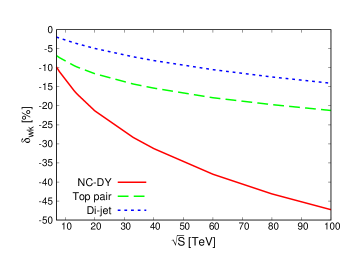
Figure 29: Relative weak corrections $\delta_{{\mathrm{wk}}}$ of Eq. (35) to the total cross sections in the high-energy region of the NC DY process (red, solid), ${\mathrm{t\bar{t}}}$ (green, dashed) and di-jet (blue, dotted) production, as a function of the proton-proton collision energy. The high-energy region is defined by a cut on the invariant mass of the leading pair of final-state particles, $M_{\rm{final}}>\sqrt{S}/4$.

Appendix: Real Corrections

MCFM uses the Catani-Seymour dipole subtraction method Catani and Seymour (1997) (and Ref. Catani et al. (2002) for massive partons) to handle the cancellation of soft and collinear singularities in NLO QCD calculations. For completeness, we present in the following the explicit expressions we used for the MCFM implementation of the real ${\cal O}(\alpha_{s})$ corrections to ${\mathrm{t\bar{t}}}$ and di-jet production at $\mathcal{O}(\alpha\alpha_{s}^{2})$. Symbolically, the corresponding cross section can be written as

$$\sigma_{real}\left(p_{a},p_{b}\right)= \int_{3}\left[d\sigma^{\mathrm{R}}\left(p_{a},p_{b},p_{1},p_{2},p_{3}\right)-\sum_{\mathrm{dipoles}}d\sigma^{\mathrm{B}}\otimes dV_{\mathrm{dipoles}}\left(p_{a},p_{b},p_{1},p_{2},p_{3}\right)\right]$$ (55)

$$+\int_{2}d\sigma^{\mathrm{B}}\left(p_{a},p_{b},p_{1},p_{2}\right)\otimes{\bf I}+\int_{2}d\sigma^{\mathrm{C}}\left(p_{a},p_{b},p_{1},p_{2}\right)\;,$$

where $p_{a}$, $p_{b}$ are the momenta of the partons in the initial state and $p_{1}$, $p_{2}$, $p_{3}$ are the momenta of the final state partons. The terms involving a convolution (denoted by the symbol $\otimes$) represent the dipole subtraction terms and their integrated versions. The two are related through the definition

$${\bf I}=\sum_{\mathrm{dipoles}}\int_{1}d\mathrm{V}_{\mathrm{dipoles}}\;.$$ (56)

$d\sigma^{R}$ denotes the contribution of the real radiation diagrams. $d\sigma^{C}$ contains the PDF counter-terms required to absorb the remaining collinear singularity into the NLO PDFs, and reads

$$d\sigma^{\mathrm{C}}_{ab}\left(p_{a},p_{b},p_{1},p_{2}\right)= -\frac{\alpha_{s}}{2\pi}\frac{\left(4\pi\right)^{\epsilon}}{\Gamma\left(1-\epsilon\right)}\sum_{c}\int dx\bigg{\{}\left[-\frac{1}{\epsilon}\left(\frac{\mu^{2}}{\mu_{F}^{2}}\right)^{\epsilon}P^{ac}\left(x\right)\right.$$ (57)

$$\left.+K^{ac}_{F.S.}\left(x\right)\right]d\sigma^{\mathrm{B}}_{cb}\left(xp_{a},p_{b},p_{1},p_{2}\right)+\left(a\leftrightarrow b\right)\bigg{\}}\;,$$

where $\mu_{F}$ is the factorization scale and $K^{ac}_{F.S.}\left(x\right)$ defines the factorization scheme. In the $\overline{\mathrm{MS}}$ scheme $K^{ac}_{F.S.}\left(x\right)=0$. $P^{ac}\left(x\right)$ are Altarelli-Parisi probabilities which can be found, for instance, in Ref. Catani and Seymour (1997).

.1 Real corrections to ${\mathrm{t\bar{t}}}$ production

In ${\mathrm{t\bar{t}}}$ production $d\sigma^{R}$ describes the diagrams of Fig. 9 and reads

$$d\sigma^{R}\propto\left|\mathcal{M}^{{\mathrm{q\bar{q}}}\rightarrow{\mathrm{t\bar{t}}}g}\right|^{2}=\left(4\pi\right)^{3}\alpha\alpha_{s}^{2}\frac{N_{\mathrm{c}}^{2}-1}{4}~{}\frac{g_{v}^{q}g_{v}^{t}\left(v_{1}+v_{2}\right)+g_{a}^{q}g_{a}^{t}\left(a_{1}+a_{2}\right)}{{\hat{s}_{15}}~{}{\hat{s}_{25}}~{}{\hat{s}_{35}}~{}{\hat{s}_{45}}~{}{\hat{s}_{12}}~{}{\hat{s}_{34}}~{}\left(\hat{s}_{12}-M_{Z}^{2}\right)~{}\left(\hat{s}_{34}-M_{Z}^{2}\right)}$$ (58)

with

$$v_{1}= ~{}8\left(\hat{t}_{1}^{2}+\hat{t}_{2}^{2}+\hat{u}_{1}^{2}+\hat{u}_{2}^{2}\right)\big{[}\hat{s}_{12}^{2}\left(\hat{t}_{1}+\hat{t}_{2}-\hat{u}_{1}-\hat{u}_{2}\right)+\hat{s}_{12}\left(\hat{t}_{1}+\hat{t}_{2}-\hat{u}_{1}-\hat{u}_{2}\right)\left(\hat{t}_{1}+\hat{t}_{2}+\hat{u}_{1}+\hat{u}_{2}\right)$$ (59)

$$+\left(\hat{t}_{1}+\hat{t}_{2}+\hat{u}_{1}+\hat{u}_{2}\right)\left(\hat{t}_{1}\hat{t}_{2}-\hat{u}_{1}\hat{u}_{2}\right)\big{]}~{}\big{[}2\hat{s}_{12}\left(\hat{s}_{12}+\hat{t}_{1}+\hat{t}_{2}+\hat{u}_{1}+\hat{u}_{2}\right)-M_{Z}^{2}\left(\hat{t}_{1}+\hat{t}_{2}+\hat{u}_{1}+\hat{u}_{2}\right)\big{]}$$

$$v_{2}= ~{}16~{}m_{t}^{2}\bigg{\{}2\hat{s}_{12}^{3}\left(\hat{t}_{1}+\hat{t}_{2}-\hat{u}_{1}-\hat{u}_{2}\right)+\hat{s}_{12}^{2}\left(\hat{t}_{1}^{2}+6\hat{t}_{1}\hat{t}_{2}+\hat{t}_{2}^{2}-\hat{u}_{1}^{2}-6\hat{u}_{1}\hat{u}_{2}-\hat{u}_{2}^{2}\right)$$

$$+\hat{s}_{12}\big{[}-\hat{t}_{1}^{3}+\hat{t}_{1}^{2}\left(3\hat{t}_{2}-\hat{u}_{1}+\hat{u}_{2}\right)+\hat{t}_{1}\left(3\hat{t}_{2}^{2}+2\hat{t}_{2}(\hat{u}_{1}+\hat{u}_{2})+\hat{u}_{1}^{2}-2\hat{u}_{1}\hat{u}_{2}-\hat{u}_{2}^{2}\right)$$

$$-\hat{t}_{2}^{3}+\hat{t}_{2}^{2}\left(\hat{u}_{1}-\hat{u}_{2}\right)+\hat{t}_{2}\left(-\hat{u}_{1}^{2}-2\hat{u}_{1}\hat{u}_{2}+\hat{u}_{2}^{2}\right)+\left(\hat{u}_{1}+\hat{u}_{2}\right)\left(\hat{u}_{1}^{2}-4\hat{u}_{1}\hat{u}_{2}+\hat{u}_{2}^{2}\right)\big{]}$$

$$-\left(\hat{t}_{1}-\hat{t}_{2}+\hat{u}_{1}-\hat{u}_{2}\right)^{2}\left(\hat{t}_{1}\hat{t}_{2}-\hat{u}_{1}\hat{u}_{2}\right)\bigg{\}}\big{[}2\hat{s}_{12}\left(\hat{s}_{12}+\hat{t}_{1}+\hat{t}_{2}+\hat{u}_{1}+\hat{u}_{2}\right)-M_{Z}^{2}\left(\hat{t}_{1}+\hat{t}_{2}+\hat{u}_{1}+\hat{u}_{2}\right)\big{]}$$

$$a_{1}= -8\left(\hat{t}_{1}^{2}+\hat{t}_{2}^{2}-\hat{u}_{1}^{2}-\hat{u}_{2}^{2}\right)\big{[}\hat{s}_{12}^{2}\left(\hat{t}_{1}+\hat{t}_{2}-\hat{u}_{1}-\hat{u}_{2}\right)+\hat{s}_{12}\left(\hat{t}_{1}+\hat{t}_{2}-\hat{u}_{1}-\hat{u}_{2}\right)\left(\hat{t}_{1}+\hat{t}_{2}+\hat{u}_{1}+\hat{u}_{2}\right)$$

$$+\left(\hat{t}_{1}+\hat{t}_{2}+\hat{u}_{1}+\hat{u}_{2}\right)\left(\hat{t}_{1}\hat{t}_{2}-\hat{u}_{1}\hat{u}_{2}\right)\big{]}~{}\big{[}2\hat{s}_{12}\left(\hat{s}_{12}+\hat{t}_{1}+\hat{t}_{2}+\hat{u}_{1}+\hat{u}_{2}\right)-M_{Z}^{2}\left(\hat{t}_{1}+\hat{t}_{2}+\hat{u}_{1}+\hat{u}_{2}\right)\big{]}$$

$$a_{2}= -32~{}m_{t}^{2}\hat{s}_{12}\left(\hat{s}_{12}+\hat{t}_{1}+\hat{u}_{1}\right)\left(\hat{s}_{12}+\hat{t}_{2}+\hat{u}_{2}\right)\left(\hat{t}_{1}+\hat{t}_{2}+\hat{u}_{1}+\hat{u}_{2}\right)$$

$$\times\left(2\hat{s}_{12}+\hat{t}_{1}+\hat{t}_{2}+\hat{u}_{1}+\hat{u}_{2}\right)\left(M_{Z}^{2}+\hat{s}_{12}+\hat{t}_{1}+\hat{t}_{2}+\hat{u}_{1}+\hat{u}_{2}\right)$$

where the Lorentz invariants are defined as

$$\hat{s}_{12}=\left(p_{q}+p_{\bar{q}}\right)^{2},\quad\hat{t}_{1}=\left(p_{q}+p_{t}\right)^{2},\quad\hat{t}_{2}=\left(p_{\bar{q}}+p_{\bar{t}}\right)^{2},\quad\hat{u}_{1}=\left(p_{q}+p_{\bar{t}}\right)^{2},\quad\hat{u}_{2}=\left(p_{\bar{q}}+p_{t}\right)^{2},$$ (60)

$$\begin{aligned} &\hat{s}_{15}=-\left(\hat{s}_{12}+\hat{t}_{1}+\hat{u}_{1}\right),\quad\hat{s}_{25}=-\left(\hat{s}_{12}+\hat{t}_{2}+\hat{u}_{2}\right),\quad\hat{s}_{35}=~{}\left(\hat{s}_{12}+\hat{t}_{2}+\hat{u}_{1}\right),\\ &\hat{s}_{45}=~{}\left(\hat{s}_{12}+\hat{t}_{1}+\hat{u}_{2}\right),\quad\hat{s}_{34}=-\left(\hat{s}_{12}+\hat{t}_{1}+\hat{t}_{2}+\hat{u}_{1}+\hat{u}_{2}+m_{t}^{2}\right).\end{aligned}$$

In this case the unintegrated dipole contribution in Eq. (55) consists of two dipoles and is given by

$$\sum_{\mathrm{dipoles}}d\sigma^{\mathrm{B}}\otimes dV_{\mathrm{dipoles}}= ~{}d\Phi_{3}\left(p_{q},p_{\bar{q}};p_{t},p_{\bar{t}},p_{g}\right)\frac{1}{S_{3}}\left\{\sum_{k=t,\bar{t}}\sum_{a=q,\bar{q}}\left[\mathcal{D}_{gk}^{a}\Theta\left(\alpha_{FI}-1+x_{gk,a}\right)\right.\right.$$ (61)

$$\left.\left.+\mathcal{D}_{k}^{ag}\Theta\left(\alpha_{IF}-u_{g}\right)\right]\right\}$$

with

$$\mathcal{D}_{gt}^{q} =-\frac{1}{\left(p_{g}+p_{t}\right)^{2}-m_{t}^{2}}\frac{1}{x_{gt,q}}\frac{1}{C_{F}}\langle\tilde{p}_{q},p_{\bar{q}},\tilde{p}_{t},p_{\bar{t}}|{\bf T}_{q}{\bf T}_{t}{\bf V}_{gt}^{q}|\tilde{p}_{q},p_{\bar{q}},\tilde{p}_{t},p_{\bar{t}}\rangle_{\alpha\alpha_{s}}$$ (62)

$$=\frac{1}{\left(p_{g}+p_{t}\right)^{2}-m_{t}^{2}}\frac{1}{x_{gt,q}}\frac{1}{C_{F}}\langle{\bf V}_{gt}^{q}\rangle\frac{N_{\mathrm{c}}^{2}-1}{4}\left|\mathcal{M}^{{\mathrm{q\bar{q}}}\rightarrow{\mathrm{t\bar{t}}}}\right|^{2}_{p_{q}\rightarrow\tilde{p}_{q},p_{t}\rightarrow\tilde{p}_{t}}$$

and

$$\mathcal{D}_{t}^{qg} =-\frac{1}{2p_{q}p_{g}}\frac{1}{x_{gt,q}}\frac{1}{C_{F}}\langle\tilde{p}_{q},p_{\bar{q}},\tilde{p}_{t},p_{\bar{t}}|{\bf T}_{t}{\bf T}_{q}{\bf V}_{t}^{qg}|\tilde{p}_{q},p_{\bar{q}},\tilde{p}_{t},p_{\bar{t}}\rangle_{\alpha\alpha_{s}}$$ (63)

$$=\frac{1}{2p_{q}p_{g}}\frac{1}{x_{gt,q}}\frac{1}{C_{F}}\langle{\bf V}_{t}^{qg}\rangle\frac{N_{\mathrm{c}}^{2}-1}{4}\left|\mathcal{M}^{{\mathrm{q\bar{q}}}\rightarrow{\mathrm{t\bar{t}}}}\right|^{2}_{p_{q}\rightarrow\tilde{p}_{q},p_{t}\rightarrow\tilde{p}_{t}}$$

These are defined in terms of

$$\langle{\bf V}_{gt}^{q}\rangle=8\pi\alpha_{s}C_{F}\left(\frac{2}{2-x_{gt,q}-\tilde{z}_{t}}-1-\tilde{z}_{t}-\frac{m_{t}^{2}}{p_{g}p_{t}}\right)$$ (64)

$$\langle{\bf V}_{t}^{qg}\rangle=8\pi\alpha_{s}C_{F}\left(\frac{2}{1-x_{gt,q}-u_{g}}-1-x_{gt,q}\right)$$

where

$$\tilde{p}^{\mu}_{q}=x_{gt,q}p^{\mu}_{q},\quad\tilde{p}^{\mu}_{t}=p^{\mu}_{g}+p^{\mu}_{t}-\left(1-x_{gt,q}\right)p^{\mu}_{q},$$

$$x_{gt,q}=\frac{p_{q}p_{g}+p_{q}p_{t}+p_{g}p_{t}}{p_{q}p_{g}+p_{q}p_{t}},\quad\tilde{z}_{t}=\frac{p_{q}p_{t}}{p_{q}p_{g}+p_{q}p_{t}},\quad u_{g}=\frac{p_{g}p_{q}}{p_{g}p_{q}+p_{t}p_{q}}.$$

$$\mathcal{D}_{gt}^{\bar{q}}=-\mathcal{D}_{gt}^{q}\left|{}_{q\leftrightarrow\bar{q}}\right.,\quad\mathcal{D}_{g\bar{t}}^{q}=-\mathcal{D}_{gt}^{q}\left|{}_{t\leftrightarrow\bar{t}}\right.,\quad\mathcal{D}_{g\bar{t}}^{\bar{q}}=\mathcal{D}_{gt}^{q}\left|{}_{q\leftrightarrow\bar{q},t\leftrightarrow\bar{t}}\right.$$ (65)

$$\mathcal{D}_{t}^{g\bar{q}}=-\mathcal{D}_{t}^{qg}\left|{}_{q\leftrightarrow\bar{q}}\right.,\quad\mathcal{D}_{\bar{t}}^{gq}=-\mathcal{D}_{t}^{qg}\left|{}_{t\leftrightarrow\bar{t}}\right.,\quad\mathcal{D}_{\bar{t}}^{g\bar{q}}=\mathcal{D}_{t}^{qg}\left|{}_{q\leftrightarrow\bar{q},t\leftrightarrow\bar{t}}\right.,$$

The occurrence of the minus sign is due to the fact that

$$\langle~{}\cdots~{}|~{}\cdots~{}{\bf T}_{\bar{q},\bar{t}}~{}\cdots~{}|~{}\cdots~{}\rangle=-~{}\langle~{}\cdots~{}|~{}\cdots~{}{\bf T}_{q,t}~{}\cdots~{}|~{}\cdots\rangle,$$

and, for the same reason, it will appear again in the case of di-jet production.

The Born matrix elements squared, $\left|\mathcal{M}^{{\mathrm{q\bar{q}}}\rightarrow{\mathrm{t\bar{t}}}}\right|^{2}$ , used in the subtraction terms are stripped of their color factors and read

$$\left|\mathcal{M}^{{\mathrm{q\bar{q}}}\rightarrow{\mathrm{t\bar{t}}}}\right|^{2}=\left(4\pi\right)^{2}\alpha\alpha_{s}\frac{8}{\hat{s}\left(\hat{s}-M_{Z}^{2}\right)}\left[g_{v}^{q}g_{v}^{t}\left(\hat{t}^{2}+\hat{u}^{2}+2m_{t}^{2}\hat{s}\right)-g_{a}^{q}g_{a}^{t}\left(\hat{t}^{2}-\hat{u}^{2}\right)\right]$$ (66)

The corresponding integrated dipoles are

$$d\sigma^{\mathrm{B}}\left(p_{q},p_{\bar{q}};p_{t},p_{\bar{t}}\right)\otimes{\bf I}= -\frac{\alpha}{2\pi}\frac{\left(4\pi\right)^{\epsilon}}{\Gamma\left(1-\epsilon\right)}\int dxd\Phi_{2}\left(xp_{q},p_{\bar{q}};p_{t},p_{\bar{t}}\right)\frac{1}{C_{F}}\times$$ (67)

$$\sum_{k=t,\bar{t}}\left[\left(-\frac{\mu^{2}}{s_{kq}}\right)^{\epsilon}{\bf I}_{k,q}\left(x,\epsilon,\mu_{kq};\alpha_{FI}\right)+\left(-\frac{\mu^{2}}{s_{qk}}\right)^{\epsilon}{\bf I}_{q,k}\left(x,\epsilon,\mu_{qk};\alpha_{IF}\right)\right]$$

$$\langle xp_{q},p_{\bar{q}},p_{t},p_{\bar{t}}|{\bf T}_{a}{\bf T}_{j}|xp_{q},p_{\bar{q}},p_{t},p_{\bar{t}}\rangle_{\alpha\alpha_{s}}+\left(q\leftrightarrow\bar{q}\right)$$

where

$${\bf I}_{t,q}\left(x,\epsilon,\mu_{tq};\alpha_{FI}\right)= ~{}\delta\left(1-x\right)~{}C_{F}~{}\Bigg{[}\frac{1}{\epsilon}\left(1+\log\frac{\mu^{2}_{tq}}{1+\mu^{2}_{tq}}\right)+\log\mu^{2}_{tq}+\frac{1}{2}\log^{2}\mu^{2}_{tq}+\frac{1}{2}\log^{2}\left(1+\mu^{2}_{tq}\right)$$ (68)

$$-2\log\mu^{2}_{tq}\log\left(1+\mu^{2}_{tq}\right)-2\mathrm{Li}_{2}\left(-\mu^{2}_{tq}\right)+2-\frac{\pi^{2}}{3}+2\log\alpha_{FI}\left(\log\frac{1+\mu^{2}_{tq}}{\mu^{2}_{tq}}-1\right)\Bigg{]}$$

$$+\Theta\left(x-1+\alpha_{FI}\right)~{}C_{F}~{}\Bigg{\{}\frac{1-x}{2\left(1-x+x\mu^{2}_{tq}\right)^{2}}+\frac{2}{1-x}\log\frac{\mu^{2}_{tq}\left(2-x+x\mu^{2}_{tq}\right)}{\left(1+\mu^{2}_{tq}\right)\left(1-x+x\mu^{2}_{tq}\right)}$$

$$+\left[\frac{2}{1-x}\left(\log\frac{1+\mu^{2}_{tq}}{\mu^{2}_{tq}}-1\right)\right]_{+}\Bigg{\}}$$

and

$${\bf I}_{q,t}\left(x,\epsilon,\mu_{qt};\alpha_{IF}\right)= ~{}\delta\left(1-x\right)~{}C_{F}~{}\Bigg{[}\frac{1}{\epsilon^{2}}+\frac{1}{\epsilon}\log\left(1+\mu^{2}_{qt}\right)-\frac{1}{2}\log^{2}\left(1+\mu^{2}_{qt}\right)+2\log\mu^{2}_{qt}\log\left(1+\mu^{2}_{qt}\right)$$ (69)

$$+2\mathrm{Li}_{2}\left(-\mu^{2}_{qt}\right)+\frac{\pi^{2}}{6}\Bigg{]}-P^{qq}_{reg}\left(x\right)\left[\frac{1}{\epsilon}-2\log\left(1-x\right)+\log{x}+\log\left(1-x+x\mu^{2}_{qt}\right)\right]$$

$$+1-x-\frac{2}{1-x}\left(\log{x}+\log\frac{2-x+x\mu^{2}_{qt}}{1+\mu^{2}_{qt}}\right)$$

$$-\Theta\left(z_{+}-\alpha_{IF}\right)~{}C_{F}~{}\bigg{[}\frac{2}{1-x}\log\frac{z_{+}\left(1-x+\alpha_{IF}\right)}{\alpha_{IF}\left(1-x+z_{+}\right)}$$

$$+P^{qq}_{reg}\left(x\right)\log\frac{z_{+}}{\alpha_{IF}}\bigg{]}-C_{F}~{}\Bigg{\{}\frac{2}{1-x}\left[\frac{1}{\epsilon}-2\log\left(1-x\right)+\log\left(1+\mu^{2}_{qt}\right)\right]\Bigg{\}}_{+}$$

with

$$s_{tq}=s_{qt}=2\tilde{p}_{t}p_{q},\quad\mu_{tq}=\mu_{qt}=\frac{m_{t}}{\sqrt{-2\tilde{p}_{t}p_{q}}},\quad z_{+}=\frac{1-x}{1-x+x\mu^{2}_{qt}}.$$ (70)

$${\bf I}_{t,\bar{q}}={\bf I}_{t,q}\left|{}_{q\leftrightarrow\bar{q}}\right.,\quad{\bf I}_{\bar{t},q}={\bf I}_{t,q}\left|{}_{t\leftrightarrow\bar{t}}\right.,\quad{\bf I}_{\bar{t},\bar{q}}={\bf I}_{t,q}\left|{}_{q\leftrightarrow\bar{q},t\leftrightarrow\bar{t}}\right.$$

$${\bf I}_{q,\bar{t}}={\bf I}_{q,t}\left|{}_{t\leftrightarrow\bar{t}}\right.,\quad{\bf I}_{\bar{q},t}={\bf I}_{q,t}\left|{}_{q\leftrightarrow\bar{q}}\right.,\quad{\bf I}_{\bar{q},\bar{t}}={\bf I}_{q,t}\left|{}_{q\leftrightarrow\bar{q},t\leftrightarrow\bar{t}}\right.$$

.2 Real corrections to di-jet production

In di-jet production at $\mathcal{O}(\alpha\alpha_{s}^{2})$ two sets of real corrections are calculated directly, those that result from the interference between $\hat{s}$- and $\hat{s}$-channel and $\hat{s}$- and $\hat{t}$-channel matrix elements. The complete real corrections for a given four-quark or two-gluon-two-quark subprocess can be expressed in terms of these two after using appropriate crossing relations. We write the two types of real correction to the $q_{i}\bar{q}_{i}\rightarrow q_{j}\bar{q}_{j}$ subprocess as

$$\left|\mathcal{M}^{q_{i}\bar{q}_{i}\rightarrow q_{j}\bar{q}_{j}g}\right|^{2}_{{\mathrm{s\times s}}} =\left(4\pi\right)^{3}\alpha\alpha_{s}^{2}\frac{N_{\mathrm{c}}^{2}-1}{4}\frac{R_{12}A^{{\mathrm{s\times s}}_{12}}+R_{34}A^{{\mathrm{s\times s}}_{34}}}{{\hat{s}_{15}}~{}{\hat{s}_{25}}~{}{\hat{s}_{35}}~{}{\hat{s}_{45}}~{}{\hat{s}_{12}}~{}{\hat{s}_{34}}~{}\left(\hat{s}_{12}-M_{V^{a}}^{2}\right)~{}\left(\hat{s}_{34}-M_{V^{a}}^{2}\right)}$$ (71)

$$\left|\mathcal{M}^{q_{i}\bar{q}_{i}\rightarrow q_{j}\bar{q}_{j}g}\right|^{2}_{{\mathrm{s\times t}}} =\left(4\pi\right)^{3}\alpha\alpha_{s}^{2}\frac{N_{\mathrm{c}}^{2}-1}{4}\frac{R_{12}A^{{\mathrm{s\times t}}_{12}}+R_{34}A^{{\mathrm{s\times t}}_{34}}}{{\hat{s}_{15}}~{}{\hat{s}_{25}}~{}{\hat{s}_{35}}~{}{\hat{s}_{45}}~{}\left(\hat{s}_{12}-M_{V^{a}}^{2}\right)~{}\left(\hat{s}_{34}-M_{V^{a}}^{2}\right)\hat{t}_{1}\hat{t}_{2}}$$

with

$$R_{12}=\frac{\left(\hat{s}_{12}-M_{V^{a}}^{2}\right)^{2}}{\left(\hat{s}_{12}-M_{V^{a}}^{2}\right)^{2}+\Gamma_{V^{a}}^{2}M_{V^{a}}^{2}},\qquad R_{34}=\frac{\left(\hat{s}_{34}-M_{V^{a}}^{2}\right)^{2}}{\left(\hat{s}_{34}-M_{V^{a}}^{2}\right)^{2}+\Gamma_{V^{a}}^{2}M_{V^{a}}^{2}}$$ (72)

and

$$A^{{\mathrm{s\times s}}_{12}}= ~{}16\hat{s}_{12}\left(\hat{s}_{34}-M_{v^{a}}^{2}\right)\bigg{[}\hat{s}_{12}^{2}\left(\hat{t}_{1}+\hat{t}_{2}-\hat{u}_{1}-\hat{u}_{2}\right)+\hat{s}_{12}\left(\hat{t}_{1}+\hat{t}_{2}-\hat{u}_{1}-\hat{u}_{2}\right)\left(\hat{t}_{1}+\hat{t}_{2}+\hat{u}_{1}+\hat{u}_{2}\right)$$ (73)

$$+\left(\hat{t}_{1}+\hat{t}_{2}+\hat{u}_{1}+\hat{u}_{2}\right)\left(\hat{t}_{1}\hat{t}_{2}-\hat{u}_{1}\hat{u}_{2}\right)\bigg{]}\bigg{[}g_{a}^{i}g_{a}^{f}\left(\hat{t}_{1}^{2}+\hat{t}_{2}^{2}-\hat{u}_{1}^{2}-\hat{u}_{2}^{2}\right)-g_{v}^{i}g_{v}^{f}\left(\hat{t}_{1}^{2}+\hat{t}_{2}^{2}+\hat{u}_{1}^{2}+\hat{u}_{2}^{2}\right)\bigg{]}$$

$$A^{{\mathrm{s\times s}}_{34}}= ~{}16\left(\hat{s}_{12}-M_{V^{a}}^{2}\right)\hat{s}_{34}\bigg{[}\hat{s}_{12}^{2}\left(\hat{t}_{1}+\hat{t}_{2}-\hat{u}_{1}-\hat{u}_{2}\right)+\hat{s}_{12}\left(\hat{t}_{1}+\hat{t}_{2}-\hat{u}_{1}-\hat{u}_{2}\right)\left(\hat{t}_{1}+\hat{t}_{2}+\hat{u}_{1}+\hat{u}_{2}\right)$$

$$+\left(\hat{t}_{1}+\hat{t}_{2}+\hat{u}_{1}+\hat{u}_{2}\right)\left(\hat{t}_{1}\hat{t}_{2}-\hat{u}_{1}\hat{u}_{2}\right)\bigg{]}\bigg{[}g_{a}^{i}g_{a}^{f}\left(\hat{t}_{1}^{2}+\hat{t}_{2}^{2}-\hat{u}_{1}^{2}-\hat{u}_{2}^{2}\right)-g_{v}^{i}g_{v}^{f}\left(\hat{t}_{1}^{2}+\hat{t}_{2}^{2}+\hat{u}_{1}^{2}+\hat{u}_{2}^{2}\right)\bigg{]}$$

$$A^{{\mathrm{s\times t}}_{12}}= ~{}\frac{16}{3}\left(\hat{s}_{34}-M_{V^{a}}^{2}\right)\left(\hat{u}_{1}^{2}+\hat{u}_{2}^{2}\right)\left(g_{a}^{i}g_{a}^{f}+g_{v}^{i}g_{v}^{f}\right)\bigg{\{}9\hat{s}_{12}^{4}+\hat{s}_{12}^{3}\left[17\hat{t}_{1}+17\hat{t}_{2}+18\left(\hat{u}_{1}+\hat{u}_{2}\right)\right]$$

$$+\hat{s}_{12}^{2}\left[8\hat{t}_{1}^{2}+\hat{t}_{1}\left(18\hat{t}_{2}+17\hat{u}_{1}+25\hat{u}_{2}\right)+8\hat{t}_{2}^{2}+\hat{t}_{2}\left(25\hat{u}_{1}+17\hat{u}_{2}\right)+9\left(\hat{u}_{1}^{2}+4\hat{u}_{1}\hat{u}_{2}+\hat{u}_{2}^{2}\right)\right]$$

$$+\hat{s}_{12}\big{[}\hat{t}_{2}\left(\hat{t}_{1}^{2}+\hat{t}_{1}\left(\hat{t}_{2}+8\hat{u}_{1}\right)+8\hat{u}_{1}\left(\hat{t}_{2}+\hat{u}_{1}\right)\right)+\hat{u}_{2}\left(25\hat{u}_{1}\left(\hat{t}_{1}+\hat{t}_{2}\right)+8\hat{t}_{1}\left(\hat{t}_{1}+\hat{t}_{2}\right)+18\hat{u}_{1}^{2}\right)$$

$$+2\hat{u}_{2}^{2}\left(4\hat{t}_{1}+9\hat{u}_{1}\right)\big{]}-\left(\hat{t}_{1}\hat{t}_{2}-\hat{u}_{1}\hat{u}_{2}\right)\left(7\hat{t}_{1}\hat{t}_{2}+8\hat{t}_{1}\hat{u}_{2}+8\hat{t}_{2}\hat{u}_{1}+9\hat{u}_{1}\hat{u}_{2}\right)\bigg{\}}$$

$$A^{{\mathrm{s\times t}}_{34}}= ~{}\frac{16}{3}\left(\hat{s}_{12}-M_{V^{a}}^{2}\right)\left(\hat{u}_{1}^{2}+\hat{u}_{2}^{2}\right)\left(g_{a}^{i}g_{a}^{f}+g_{v}^{i}g_{v}^{f}\right)\bigg{\{}9\hat{s}_{12}^{4}+\hat{s}_{12}^{3}\left[19\hat{t}_{1}+19\hat{t}_{2}+18\left(\hat{u}_{1}+\hat{u}_{2}\right)\right]$$

$$+\hat{s}_{12}^{2}\left[11\hat{t}_{1}^{2}+4\hat{t}_{1}\left(6\hat{t}_{2}+7\hat{u}_{1}+5\hat{u}_{2}\right)+11\hat{t}_{2}^{2}+4\hat{t}_{2}\left(5\hat{u}_{1}+7\hat{u}_{2}\right)+9\left(\hat{u}_{1}^{2}+4\hat{u}_{1}\hat{u}_{2}+\hat{u}_{2}^{2}\right)\right]$$

$$+\hat{s}_{12}\big{[}\hat{t}_{1}^{3}+2\hat{t}_{1}^{2}\left(3\hat{t}_{2}+5\hat{u}_{1}+\hat{u}_{2}\right)+\hat{t}_{1}\left(6\hat{t}_{2}^{2}+16\hat{t}_{2}\left(\hat{u}_{1}+\hat{u}_{2}\right)+9\hat{u}_{1}^{2}+29\hat{u}_{1}\hat{u}_{2}+\hat{u}_{2}^{2}\right)$$

$$+9\hat{u}_{2}^{2}\left(\hat{t}_{2}+2\hat{u}_{1}\right)+\hat{u}_{2}\left(\hat{t}_{2}+2\hat{u}_{1}\right)\left(10\hat{t}_{2}+9\hat{u}_{1}\right)+\hat{t}_{2}\left(\hat{t}_{2}+\hat{u}_{1}\right)^{2}\big{]}+\hat{u}_{2}\big{[}\hat{t}_{1}^{2}\left(3\hat{t}_{2}+\hat{u}_{1}\right)$$

$$-\hat{t}_{1}\left(5\hat{t}_{2}-9\hat{u}_{1}\right)\left(\hat{t}_{2}+\hat{u}_{1}\right)+\hat{t}_{2}\hat{u}_{1}\left(\hat{t}_{2}+\hat{u}_{1}\right)\big{]}+\hat{t}_{1}\hat{t}_{2}\left[\hat{t}_{1}^{2}-5\hat{t}_{1}\left(\hat{t}_{2}+\hat{u}_{1}\right)+\left(\hat{t}_{2}+\hat{u}_{1}\right)\left(\hat{t}_{2}+2\hat{u}_{1}\right)\right]$$

$$+\hat{u}_{2}^{2}\left[\hat{t}_{1}(2\hat{t}_{2}+\hat{u}_{1})+9\hat{u}_{1}\left(\hat{t}_{2}+\hat{u}_{1}\right)\right]\bigg{\}}\;,$$

where $g_{v}^{f}(g_{a}^{f})$ denote the vector(axial) vector coupling, $M_{V^{a}}$ the mass, and $\Gamma_{V^{a}}$ the total decay width of the weak gauge boson. The Lorentz invariants are defined as

$$\hat{s}_{12}=\left(p_{q_{i}}+p_{\bar{q}_{i}}\right)^{2},\quad\hat{t}_{1}=\left(p_{q_{i}}+p_{q_{j}}\right)^{2},\quad\hat{t}_{2}=\left(p_{\bar{q}_{i}}+p_{\bar{q}_{j}}\right)^{2},\quad\hat{u}_{1}=\left(p_{q_{i}}+p_{\bar{q}_{j}}\right)^{2},\quad\hat{u}_{2}=\left(p_{\bar{q}_{i}}+p_{q_{j}}\right)^{2},$$ (74)

$$\begin{aligned} &\hat{s}_{15}=-\left(\hat{s}_{12}+\hat{t}_{1}+\hat{u}_{1}\right),\quad\hat{s}_{25}=-\left(\hat{s}_{12}+\hat{t}_{2}+\hat{u}_{2}\right),\quad\hat{s}_{35}=~{}\left(\hat{s}_{12}+\hat{t}_{2}+\hat{u}_{1}\right),\\ &\hat{s}_{45}=~{}\left(\hat{s}_{12}+\hat{t}_{1}+\hat{u}_{2}\right),\quad\hat{s}_{34}=-\left(\hat{s}_{12}+\hat{t}_{1}+\hat{t}_{2}+\hat{u}_{1}+\hat{u}_{2}\right).\end{aligned}$$

The real corrections to the subprocesses with quark-gluon initial states can be obtained from Eq. (71) by applying the following crossing symmetries:

$$\left|\mathcal{M}^{q_{i}g\rightarrow q_{i}q_{j}\bar{q}_{j}}\right|^{2}=-\left|\mathcal{M}^{q_{i}\bar{q}_{i}\rightarrow q_{j}\bar{q}_{j}g}\right|^{2}_{s_{12}\rightarrow t_{1},~{}t_{1}\rightarrow u_{1},~{}t_{2}\rightarrow s_{35},~{}u_{1}\rightarrow s_{15},~{}u_{2}\rightarrow s_{34}}$$ (75)

$$\left|\mathcal{M}^{\bar{q}_{i}g\rightarrow\bar{q}_{i}q_{j}\bar{q}_{j}}\right|^{2}=-\left|\mathcal{M}^{q_{i}\bar{q}_{i}\rightarrow q_{j}\bar{q}_{j}g}\right|^{2}_{s_{12}\rightarrow t_{1},~{}t_{1}\rightarrow s_{35},~{}t_{2}\rightarrow u_{1},~{}u_{1}\rightarrow s_{34},~{}u_{2}\rightarrow s_{15}}$$

$$\left|\mathcal{M}^{gq_{i}\rightarrow q_{j}q_{i}\bar{q}_{j}}\right|^{2}=-\left|\mathcal{M}^{q_{i}\bar{q}_{i}\rightarrow q_{j}\bar{q}_{j}g}\right|^{2}_{s_{12}\rightarrow s_{35},~{}t_{1}\rightarrow s_{45},~{}t_{2}\rightarrow u_{2},~{}u_{1}\rightarrow s_{25},~{}u_{2}\rightarrow s_{34}}$$

$$\left|\mathcal{M}^{g\bar{q}_{i}\rightarrow\bar{q}_{j}\bar{q}_{i}q_{j}}\right|^{2}=-\left|\mathcal{M}^{q_{i}\bar{q}_{i}\rightarrow q_{j}\bar{q}_{j}g}\right|^{2}_{s_{12}\rightarrow s_{35},~{}t_{1}\rightarrow u_{2},~{}t_{2}\rightarrow s_{45},~{}u_{1}\rightarrow s_{34},~{}u_{2}\rightarrow s_{25}}$$

The unintegrated dipole contribution in Eq. (55) for the $q_{i}\bar{q}_{i}\rightarrow q_{j}\bar{q}_{j}$ subprocesses consist of four dipoles that are written as follows:

$$\sum_{\mathrm{dipoles}}d\sigma^{\mathrm{B}}\otimes dV_{\mathrm{dipoles}}= ~{}d\Phi_{3}\left(p_{q_{i}},p_{\bar{q}_{i}};p_{q_{j}},p_{\bar{q}_{j}},p_{g}\right)\frac{1}{S_{3}}\bigg{\{}\sum_{k,l=q_{j},\bar{q}_{j}}^{k\neq l}\mathcal{D}_{gk,l}\Theta\left(\alpha_{FF}-y_{gk,l}\right)$$ (76)

$$+\sum_{k=q_{j},\bar{q}_{j}}\sum_{a=q_{i},\bar{q}_{i}}\left[\mathcal{D}_{gk}^{a}\Theta\left(\alpha_{FI}-1+x_{gk,a}\right)+\mathcal{D}_{k}^{ag}\Theta\left(\alpha_{IF}-u_{g}\right)\right]$$

$$+\sum_{a=q_{i},\bar{q}_{i}}\sum_{b=q_{i},\bar{q}_{i}}^{a\neq b}\mathcal{D}^{ag,b}\Theta\left(\alpha_{II}-\tilde{v}_{g}\right)\bigg{\}}$$

with

$$\mathcal{D}_{gq_{j},\bar{q}_{j}} = -\frac{1}{2p_{g}p_{q_{j}}}\frac{1}{C_{F}}\langle{\bf V}_{gq_{j},\bar{q}_{j}}\rangle\langle p_{q_{i}},p_{\bar{q}_{i}},\tilde{p}_{q_{j}},\tilde{p}_{\bar{q}_{j}}|{\bf T}_{\bar{q}_{j}}{\bf T}_{q_{j}}|p_{q_{i}},p_{\bar{q}_{i}},\tilde{p}_{q_{j}},\tilde{p}_{\bar{q}_{j}}\rangle_{\alpha\alpha_{s}}$$

$$\mathcal{D}_{gq_{j}}^{q_{i}} = -\frac{1}{2p_{g}p_{q_{j}}}\frac{1}{x_{gq_{j},q_{i}}}\frac{1}{C_{F}}\langle{\bf V}_{gq_{j}}^{q_{i}}\rangle\langle\tilde{p}_{q_{i}},p_{\bar{q}_{i}},\tilde{p}_{q_{j}},p_{\bar{q}_{j}}|{\bf T}_{q_{i}}{\bf T}_{q_{j}}|\tilde{p}_{q_{i}},p_{\bar{q}_{i}},\tilde{p}_{q_{j}},p_{\bar{q}_{j}}\rangle_{\alpha\alpha_{s}}$$

$$\mathcal{D}^{q_{i}g}_{q_{j}} = \frac{1}{2p_{q_{i}}p_{g}}\frac{1}{x_{gq_{j},q_{i}}}\frac{1}{C_{F}}\langle{\bf V}^{q_{i}g}_{q_{j}}\rangle\langle\tilde{p}_{q_{i}},p_{\bar{q}_{i}},\tilde{p}_{q_{j}},p_{\bar{q}_{j}}|{\bf T}_{q_{j}}{\bf T}_{q_{i}}|\tilde{p}_{q_{i}},p_{\bar{q}_{i}},\tilde{p}_{q_{j}},p_{\bar{q}_{j}}\rangle_{\alpha\alpha_{s}}$$

$$\mathcal{D}^{q_{i}g,\bar{q}_{i}} = \frac{1}{2p_{q_{i}}p_{g}}\frac{1}{x_{g,q_{i}\bar{q}_{i}}}\frac{1}{C_{F}}\langle{\bf V}^{q_{i}g,\bar{q}_{i}}\rangle\langle\tilde{p}_{q_{i}},p_{\bar{q}_{i}},\tilde{p}_{q_{j}},\tilde{p}_{\bar{q}_{j}}|{\bf T}_{\bar{q}_{i}}{\bf T}_{q_{i}}|\tilde{p}_{q_{i}},p_{\bar{q}_{i}},\tilde{p}_{q_{j}},\tilde{p}_{\bar{q}_{j}}\rangle_{\alpha\alpha_{s}}\;.$$ (77)

These are defined in terms of

$$\langle{\bf V}_{gq_{j},\bar{q}_{j}}\rangle=8\pi\alpha_{s}C_{F}\left(\frac{2}{1-\tilde{z}_{q_{j}}\left(1-y_{gq_{j},\bar{q}_{j}}\right)}-1-\tilde{z}_{q_{j}}\right),$$ (78)

$$\tilde{p}_{q_{j}}^{\mu}=p_{q_{j}}^{\mu}+p_{g}^{\mu}-\frac{y_{gq_{j},\bar{q}_{j}}}{1-y_{gq_{j},\bar{q}_{j}}}p_{\bar{q}_{j}},\quad\tilde{p}_{\bar{q}_{j}}=\frac{1}{1-y_{gq_{j},\bar{q}_{j}}}p_{\bar{q}_{j}},$$

$$y_{gq_{j},\bar{q}_{j}}=\frac{p_{g}p_{q_{j}}}{p_{g}p_{q_{j}}+p_{q_{j}}p_{\bar{q}_{j}}+p_{\bar{q}_{j}}p_{g}},\quad\tilde{z}_{q_{j}}=\frac{p_{q_{j}}p_{\bar{q}_{j}}}{p_{g}p_{\bar{q}_{j}}+p_{q_{j}}p_{\bar{q}_{j}}}.$$

$$\langle{\bf V}_{gq_{j}}^{q_{i}}\rangle=8\pi\alpha_{s}C_{F}\left(\frac{2}{2-x_{gq_{j},q_{i}}-\tilde{z}_{q_{j}}}-1-\tilde{z}_{q_{j}}\right),$$ (79)

$$\tilde{p}_{q_{i}}^{\mu}=x_{gq_{j},q_{i}}p_{q_{i}}^{\mu},\quad\tilde{p}_{q_{j}}^{\mu}=p_{q_{j}}^{\mu}+p_{g}^{\mu}-\left(1-x_{gq_{j},q_{i}}\right)p_{q_{i}}^{\mu},$$

$$x_{gq_{j},q_{i}}=\frac{p_{gq_{j},q_{i}}p_{q_{i}}+p_{g}p_{q_{i}}+p_{q_{j}}p_{g}}{p_{q_{j}}p_{q_{i}}+p_{g}p_{q_{i}}},\quad\tilde{z}_{q_{j}}=\frac{p_{q_{j}}p_{q_{i}}}{p_{q_{j}}p_{q_{i}}+p_{g}p_{q_{i}}}.$$

$$\langle{\bf V}_{q_{j}}^{q_{i}g}\rangle=8\pi\alpha_{s}C_{F}\left(\frac{2}{1-x_{gq_{j},q_{g}}-u_{g}}-1-x_{gq_{j},q_{i}}\right),$$ (80)

$$\tilde{p}_{q_{i}}^{\mu}=x_{gq_{j},q_{g}}p_{q_{i}}^{\mu},\quad\tilde{p}_{q_{j}}^{\mu}=p_{q_{j}}^{\mu}+p_{g}^{\mu}-\left(1-x_{gq_{j},q_{g}}\right)p_{q_{i}}^{\mu},$$

$$x_{gq_{j},q_{g}}=\frac{p_{q_{j}}p_{q_{i}}+p_{g}p_{q_{i}}+p_{g}p_{q_{j}}}{p_{q_{j}}p_{q_{i}}+p_{g}p_{q_{i}}},\quad u_{g}=\frac{p_{g}p_{q_{i}}}{p_{g}p_{q_{i}}+p_{q_{j}}p_{q_{i}}}.$$

$$\langle{\bf V}^{q_{i}g,\bar{q}_{i}}\rangle=8\pi\alpha_{s}C_{F}\left(\frac{2}{1-x_{g,q_{i}\bar{q}_{i}}}-1-x_{g,q_{i}\bar{q}_{i}}\right),$$ (81)

$$\tilde{p}_{q_{i}}^{\mu}=x_{g,q_{i}\bar{q}_{i}}p_{q_{i}}^{\mu},\quad\tilde{p}_{q_{j}(\bar{q}_{j})}^{\mu}=p_{q_{j}(\bar{q}_{j})}^{\mu}-\frac{2p_{q_{j}(\bar{q}_{j})}\cdot\left(K+\tilde{K}\right)}{\left(K+\tilde{K}\right)^{2}}\left(K+\tilde{K}\right)^{\mu}+\frac{2p_{q_{j}(\bar{q}_{j})}\cdot K}{K^{2}}\tilde{K}^{\mu},$$

$$x_{g,q_{i}\bar{q}_{i}}=\frac{p_{q_{i}}p_{\bar{q}_{i}}+p_{g}p_{q_{i}}+p_{g}p_{\bar{q}_{i}}}{p_{q_{i}}p_{\bar{q}_{i}}},\quad K^{\mu}=p_{q_{i}}^{\mu}+p_{\bar{q}_{i}}^{\mu}+p_{g}^{\mu},\quad\tilde{K}^{\mu}=\tilde{p}_{q_{i}}^{\mu}+p_{\bar{q}_{i}}^{\mu},\quad\tilde{v}_{g}=-\frac{p_{q_{i}}p_{g}}{p_{q_{i}}p_{\bar{q}_{i}}}$$

The remaining dipole contributions can be obtained via the relations

$$\mathcal{D}_{g\bar{q}_{j},q_{j}}=\mathcal{D}_{gq_{j},\bar{q}_{j}}\left|{}_{q_{j}\leftrightarrow\bar{q}_{j}}\right.,\quad\mathcal{D}^{\bar{q}_{i}g,q_{i}}=\mathcal{D}^{q_{i}g,\bar{q}_{i}}\left|{}_{q_{i}\leftrightarrow\bar{q}_{i}}\right.$$ (82)

$$\mathcal{D}_{gq_{j}}^{\bar{q}_{i}}=-\mathcal{D}_{gq_{j}}^{q_{i}}\left|{}_{q_{i}\leftrightarrow\bar{q}_{i}}\right.,\quad\mathcal{D}_{g\bar{q}_{j}}^{q_{i}}=-\mathcal{D}_{gq_{j}}^{q_{i}}\left|{}_{q_{j}\leftrightarrow\bar{q}_{j}}\right.,\quad\mathcal{D}_{g\bar{q}_{j}}^{\bar{q}_{i}}=\mathcal{D}_{gq_{j}}^{q_{i}}\left|{}_{q_{i}\leftrightarrow\bar{q}_{i},q_{j}\leftrightarrow\bar{q}_{j}}\right.$$

$$\mathcal{D}_{q_{j}}^{\bar{q}_{i}g}=-\mathcal{D}_{q_{j}}^{q_{i}g}\left|{}_{q_{i}\leftrightarrow\bar{q}_{i}}\right.,\quad\mathcal{D}_{\bar{q}_{j}}^{q_{i}g}=-\mathcal{D}_{q_{j}}^{q_{i}g}\left|{}_{q_{j}\leftrightarrow\bar{q}_{j}}\right.,\quad\mathcal{D}_{\bar{q}_{j}}^{\bar{q}_{i}g}=\mathcal{D}_{q_{j}}^{q_{i}g}\left|{}_{q_{i}\leftrightarrow\bar{q}_{i},q_{j}\leftrightarrow\bar{q}_{j}}\right.$$

The following Born matrix elements squared stripped of their color factors are to be used in these subtraction terms:

$$\left|\mathcal{M}^{q_{i}\bar{q}_{i}\rightarrow q_{j}\bar{q}_{j}}\right|^{2}_{{\mathrm{s\times s}}} =\left(4\pi\right)^{2}\alpha\alpha_{s}\frac{\mathrm{prop}_{V^{a}}\left(\hat{s}\right)}{\hat{s}^{2}}~{}8~{}\left[g_{v}^{i}g_{v}^{f}\left(\hat{t}^{2}+\hat{u}^{2}\right)-g_{a}^{i}g_{a}^{f}\left(\hat{t}^{2}-\hat{u}^{2}\right)\right]$$ (83)

$$\left|\mathcal{M}^{q_{i}\bar{q}_{i}\rightarrow q_{j}\bar{q}_{j}}\right|^{2}_{{\mathrm{s\times t}}} =\left(4\pi\right)^{2}\alpha\alpha_{s}\frac{\mathrm{prop}_{V^{a}}\left(\hat{s}\right)}{\hat{s}\hat{t}}~{}8~{}\left(g_{v}^{i}g_{v}^{f}+g_{a}^{i}g_{a}^{f}\right)\hat{u}^{2}$$

with $\mathrm{prop}_{V^{a}}(\hat{s})$ of Eq. (16). The integrated dipoles are combined according to

$$d\sigma^{\mathrm{B}}\left(p_{q_{i}},p_{\bar{q}_{i}};p_{q_{j}},p_{\bar{q}_{j}}\right)\otimes{\bf I}= -\frac{\alpha}{2\pi}\frac{\left(4\pi\right)^{\epsilon}}{\Gamma\left(1-\epsilon\right)}\int dxd\Phi_{2}\left(xp_{q_{i}},p_{\bar{q}_{i}};p_{q_{j}},p_{\bar{q}_{j}}\right)\frac{1}{C_{F}}\times\Bigg{\{}$$ (84)

$$\left(\frac{\mu^{2}}{s_{q_{i}\bar{q}_{i}}}\right)^{\epsilon}{\bf I}_{q_{i},\bar{q}_{i}}\left(x,\epsilon;\alpha_{II}\right)+\sum_{k,l=q_{j},\bar{q}_{j}}^{k\neq l}\left(\frac{\mu^{2}}{s_{kl}}\right)^{\epsilon}{\bf I}_{k,l}\left(x,\epsilon;\alpha_{FF}\right)$$

$$+\sum_{k=q_{j},\bar{q}_{j}}\bigg{[}\left(-\frac{\mu^{2}}{s_{kq_{i}}}\right)^{\epsilon}{\bf I}_{k,q_{i}}\left(x,\epsilon;\alpha_{FI}\right)+\left(-\frac{\mu^{2}}{s_{q_{i}k}}\right)^{\epsilon}{\bf I}_{q_{i},k}\left(x,\epsilon;\alpha_{IF}\right)\bigg{]}\Bigg{\}}$$

$$\times\langle xp_{q_{i}},p_{\bar{q}_{i}},p_{q_{j}},p_{\bar{q}_{j}}|{\bf T}_{k}{\bf T}_{l}|xp_{q_{i}},p_{\bar{q}_{i}},p_{q_{j}},p_{\bar{q}_{j}}\rangle_{\alpha\alpha_{s}}+\left(q\leftrightarrow\bar{q}\right)$$

where the four types of contribution can be written as

$${\bf I}_{q_{i},\bar{q}_{i}}\left(x,\epsilon;\alpha_{II}\right)= ~{}C_{F}\Bigg{\{}\delta\left(1-x\right)\left(\frac{1}{\epsilon^{2}}-\frac{\pi^{2}}{6}\right)+1-x+\left(1+x\right)\left[\frac{1}{\epsilon}-2\log\left(1-x\right)\right]$$ (85)

$$-\frac{1+x^{2}}{1-x}\big{[}\log{x}-\log\alpha_{II}\left(x\right)\big{]}-\bigg{\{}\frac{2}{1-x}\left[\frac{1}{\epsilon}-2\log\left(1-x\right)\right]\bigg{\}}_{+}\Bigg{\}}$$

$${\bf I}_{q_{j},\bar{q}_{j}}\left(x,\epsilon;\alpha_{FF}\right)=~{}C_{F}\Bigg{\{}\delta\left(1-x\right)\left[\frac{1}{\epsilon^{2}}+\frac{3}{2\epsilon}+\frac{7}{2}-\frac{\pi^{2}}{2}+\frac{3}{2}\left(\alpha_{FF}-\log\alpha_{FF}\right)-\log^{2}\alpha_{FF}\right]\Bigg{\}}$$ (86)

$${\bf I}_{q_{j},q_{i}}\left(x,\epsilon;\alpha_{FI}\right)= ~{}C_{F}\Bigg{\{}\delta\left(1-x\right)\left[\frac{1}{\epsilon^{2}}+\frac{3}{2\epsilon}+\frac{7}{2}-\frac{\pi^{2}}{2}-\log\alpha_{FI}\left(\log\alpha_{FI}+\frac{3}{2}\right)\right]$$ (87)

$$+\Theta\left(x-1+\alpha_{FI}\right)\bigg{\{}\frac{2}{1-x}\log\left(2-x\right)-\frac{3}{2}\left(\frac{1}{1-x}\right)_{+}-\left[\frac{2}{1-x}\log\left(1-x\right)\right]_{+}\bigg{\}}\Bigg{\}}$$

$${\bf I}_{q_{i},q_{j}}\left(x,\epsilon;\alpha_{IF}\right)= ~{}C_{F}\Bigg{\{}\delta\left(1-x\right)\left(\frac{1}{\epsilon^{2}}+\frac{\pi^{2}}{6}\right)+\left(1+x\right)\left[\frac{1}{\epsilon}-\log\left(1-x\right)\right]+1-x-\frac{1+x^{2}}{1-x}\log{x}$$ (88)

$$-\frac{2}{1-x}\log\frac{1-x+\alpha_{IF}}{\alpha_{IF}}-\left(1+x\right)\log\alpha_{IF}-\bigg{\{}\frac{2}{1-x}\left[\frac{1}{\epsilon}-2\log\left(1-x\right)\right]\bigg{\}}_{+}\Bigg{\}}$$

$${\bf I}_{\bar{q}_{j},q_{j}}={\bf I}_{q_{j},\bar{q_{j}}},\quad{\bf I}_{\bar{q}_{i},q_{i}}={\bf I}_{q_{i},\bar{q}_{i}}$$ (89)

$${\bf I}_{q_{j},\bar{q}_{i}}={\bf I}_{\bar{q}_{j},q_{i}}={\bf I}_{\bar{q}_{j},\bar{q}_{i}}={\bf I}_{q_{j},q_{i}}$$

$${\bf I}_{q_{i},\bar{q}_{j}}={\bf I}_{\bar{q}_{i},q_{j}}={\bf I}_{\bar{q}_{i},\bar{q}_{j}}={\bf I}_{q_{i},q_{j}}$$

The $\alpha_{II}(x)$ function is defined as follows,

$$\alpha_{II}\left(x\right)=\mathrm{min}\left\{\frac{\alpha_{II}}{1-x},1\right\}\,,$$ (90)

where $\alpha_{K},K=II,IF,FI,FF$ is a variable which can be used to limit the kinematic range for the subtraction of initial-initial ($K=II$), initial-final ($K=IF,FI$), and final-final ($K=FF$) dipoles as suggested in Ref. Nagy (2003). $\alpha_{K}=1$ corresponds to standard Catani-Seymour subtraction. The Altarelli-Parisi function for the $q\rightarrow gq$ splitting reads

$$P^{qq}\left(x\right)=\frac{3}{2}C_{F}\delta\left(1-x\right)+P^{qq}_{reg}\left(x\right)+2C_{F}\left(\frac{1}{1-x}\right)_{+},$$ (91)

with

$$P^{qq}_{reg}=-C_{F}\left(1+x\right).$$

The real corrections in the quark-gluon-initiated subprocesses in the two-gluon-two-quark category shown in Table 2 (processes B-E) only exhibit initial-state collinear divergences that are eventually absorbed into corresponding PDF counterterms. The unintegrated dipole contribution to these subprocesses at $\mathcal{O}(\alpha\alpha_{s}^{2})$, given in Eq. (55), consists of two dipoles that can be written as:

$$\sum_{\mathrm{dipoles}}d\sigma^{\mathrm{B}}\otimes dV_{\mathrm{dipoles}}= ~{}d\Phi_{3}\left(p_{g},p_{\bar{q}_{i}};p_{q_{j}},p_{\bar{q}_{j}},p_{\bar{q}_{i}}\right)\frac{1}{S_{3}}\Big{\{}\mathcal{D}^{g\bar{q}_{i},\bar{q}_{i}}\Theta\left(\alpha_{II}-\tilde{v}_{\bar{q}_{i}}\right)\Big{\}}+\left(q_{i}\leftrightarrow\bar{q}_{i}\right)$$ (92)

with

$$\mathcal{D}^{g\bar{q}_{i},\bar{q}_{i}} = \frac{1}{2p_{g}p_{\bar{q}_{i}}}\frac{1}{x_{\bar{q}_{i},gq_{i}}}\frac{1}{C_{F}}\langle{\bf V}^{g\bar{q}_{i},\bar{q}_{i}}\rangle\langle\tilde{p}_{q_{i}},p_{\bar{q}_{i}},\tilde{p}_{q_{j}},\tilde{p}_{\bar{q}_{j}}|{\bf T}_{q_{i}}{\bf T}_{\bar{q}_{i}}|p_{q_{i}},\tilde{p}_{\bar{q}_{i}},\tilde{p}_{q_{j}},\tilde{p}_{\bar{q}_{j}}\rangle_{\alpha\alpha_{s}}\;,$$ (93)

where

$$\langle{\bf V}^{g\bar{q}_{i},\bar{q}_{i}}\rangle=8\pi\alpha_{s}T_{R}\left(1-2x_{\bar{q}_{i},g\bar{q}_{i}}-2x_{\bar{q}_{i},g\bar{q}_{i}}^{2}\right),$$ (94)

$$\tilde{p}_{q_{i}}^{\mu}=x_{\bar{q}_{i},g\bar{q}_{i}}p_{g}^{\mu},\quad\tilde{p}_{q_{j}(\bar{q}_{j})}^{\mu}=p_{q_{j}(\bar{q}_{j})}^{\mu}-\frac{2p_{q_{j}(\bar{q}_{j})}\cdot\left(K+\tilde{K}\right)}{\left(K+\tilde{K}\right)^{2}}\left(K+\tilde{K}\right)^{\mu}+\frac{2p_{q_{j}(\bar{q}_{j})}\cdot K}{K^{2}}\tilde{K}^{\mu},$$

$$x_{\bar{q}_{i},g\bar{q}_{i}}=\frac{2p_{g}p_{\bar{q}_{i}}+p_{\bar{q}_{i}}^{2}}{p_{g}p_{\bar{q}_{i}}},\quad K^{\mu}=p_{g}^{\mu}+2p_{\bar{q}_{i}}^{\mu},\quad\tilde{K}^{\mu}=\tilde{p}_{q_{i}}^{\mu}+p_{\bar{q}_{i}}^{\mu},\quad\tilde{v}_{\bar{q}_{i}}=-1$$

$$\mathcal{D}^{gq_{i},q_{i}}=\mathcal{D}^{g\bar{q}_{i},\bar{q}_{i}}\left|{}_{q_{i}\leftrightarrow\bar{q}_{i}}\right.$$

The contribution of the corresponding integrated dipoles reads:

$$d\sigma^{\mathrm{B}}\left(p_{g},p_{\bar{q}_{i}};p_{q_{j}},p_{\bar{q}_{j}}\right)\otimes{\bf I}+\left(q_{i}\leftrightarrow\bar{q}_{i}\right)=-\frac{\alpha}{2\pi}\frac{\left(4\pi\right)^{\epsilon}}{\Gamma\left(1-\epsilon\right)}\int dxd\Phi_{2}\left(xp_{g},p_{\bar{q}_{i}};p_{q_{j}},p_{\bar{q}_{j}}\right)\frac{1}{C_{F}}\times\Bigg{\{}$$ (95)

$$\left(\frac{\mu^{2}}{s_{g\bar{q}_{i}}}\right)^{\epsilon}{\bf I}_{g,\bar{q}_{i}}\left(x,\epsilon;\alpha_{II}\right)\langle xp_{g}(p_{q_{i}}),p_{\bar{q}_{i}},p_{q_{j}},p_{\bar{q}_{j}}|{\bf T}_{q_{i}}{\bf T}_{\bar{q}_{i}}|xp_{g}(p_{q_{i}}),p_{\bar{q}_{i}},p_{q_{j}},p_{\bar{q}_{j}}\rangle_{\alpha\alpha_{s}}\Bigg{\}}+\left(q_{i}\leftrightarrow\bar{q}_{i}\right)$$

with

$${\bf I}_{g,\bar{q}_{i}}\left(x,\epsilon;\alpha_{II}\right)={\bf I}_{g,q_{i}}\left(x,\epsilon;\alpha_{II}\right)= ~{}T_{R}~{}\bigg{\{}\left[\left(1-x\right)^{2}+x^{2}\right]\left[2\log\left(1-x\right)-\log{x}-\frac{1}{\epsilon}\right]+2x-2x^{2}$$ (96)

$$+\left[\left(1-x\right)^{2}+x^{2}\right]\log\alpha_{II}\left(x\right)\bigg{\}}\;,$$

where the $\alpha_{II}(x)$ function is defined in Eq. (90) and the Altarelli-Parisi function for the $g\rightarrow q\bar{q}$ splitting reads

$$P^{gq}\left(x\right)=P^{gq}_{reg}\left(x\right)=T_{R}\left[\left(1-x\right)^{2}+x^{2}\right]\;.$$ (97)