Galactoseismology and the Local Density of Dark Matter

Abstract

We model vertical breathing mode perturbations in the Milky Way’s stellar disc and study their effects on estimates of the local dark matter density, surface density, and vertical force. Evidence for these perturbations, which involve compression and expansion of the Galactic disc perpendicular to its midplane, come from the SEGUE, RAVE, and LAMOST surveys. We show that their existence may lead to systematic errors of $10\%$ or greater in the vertical force $K_{z}(z)$ at $|z|=1.1\,{\rm kpc}$. These errors translate to $\ga 25\%$ errors in estimates of the local dark matter density. Using different mono-abundant subpopulations as tracers offers a way out: if the inferences from all tracers in the Gaia era agree, then the dark matter determination will be robust. Disagreement in the inferences from different tracers will signal the breakdown of the unperturbed model and perhaps provide the means for determining the nature of the perturbation.

1 Introduction

In his seminal work on the vertical structure of the Galaxy, Oort (1932) introduced a method to determine the gravitational force perpendicular to the Galactic plane (the vertical force) near the Sun from stellar kinematics. Though Oort’s main interest was in developing a dynamical model for the Galaxy, he recognized that a measurement of the vertical force as a function of distance from the midplane could be combined with estimates of the density in visible matter to infer the existence of unseen “dark matter”. To be sure, his concept of dark matter was not what it is today. Nevertheless, the Oort problem, as efforts to determine the vertical structure of the Milky Way have come to be known, provides our best astrophysical handle on the local density of dark matter.

The Oort problem relies on astrometric observations of stars that act as tracers of the gravitational potential. A key assumption is that the tracers are in dynamical equilibrium with respect to their vertical motions (Bahcall, 1984a, b; Bienayme et al., 1987; Kuijken & Gilmore, 1989a, b, c, 1991; Holmberg & Flynn, 2000, 2004; Bovy & Tremaine, 2012; Garbari et al., 2012; Bovy & Rix, 2013); for a recent review, see Read (2014). The assumption that the Galaxy is a steady state system dates back to Jeans (1922) in his critique of Kapteyn’s Galactic model (Kapteyn 1922) and was central to Oort’s analysis of the Galaxy’s vertical structure. This assumption is plausible since a typical star will have completed many oscillations through the Galactic midplane over its lifetime. The discoveries of bulk vertical motions in the stellar disc (Widrow et al., 2012; Williams et al., 2013; Carlin et al., 2013) and a North-South asymmetry in the number counts of solar neighbourhood stars (Widrow et al., 2012; Yanny & Gardner, 2013) call into question this assumption. In particular, the bulk motion observations imply that the disc is undergoing compression and expansion perpendicular to the midplane, in essence, a localized breathing mode. Depending on its phase, the breathing mode may manifest itself as a correlation between the mean vertical velocity of the tracers and distance from the midplane. Indeed, the observations mentioned above suggest that variations in the mean velocity with $z$ are of order $4-8\,{\rm km\,s}^{-1}{\rm kpc}^{-1}$. Perturbations of this type can be caused by the passage of a globular cluster, dwarf galaxy, or dark matter sub-halo through the disc plane (Widrow et al., 2012; Gómez et al., 2013; Widrow et al., 2014; Feldmann & Spolyar, 2015) or by gravitational effects of a passing spiral arm (Faure et al., 2014; Debattista, 2014).

In this paper, we investigate the impact of a breathing mode perturbation on efforts to determine the local vertical force and dark matter density. If the entire stellar disc participates in a breathing mode, then the surface density of stars within a particular distance from the Galactic midplane, and therefore the vertical force, will change with time. Furthermore, if a tracer population participates in a breathing mode, then models that treat it as an equilibrium system will yield erroneous results for the inferred vertical force.

It is common practice to use $K_{1.1}$, the magnitude of the vertical force $1.1\,{\rm kpc}$ above and below midplane of the disk at the Sun’s position, as a dynamical constraint on the structure of the Galaxy. Much closer to the midplane and baryons will dominate the vertical gravitational force. Much further from the midplane and halo stars will contaminate the sample of tracers. As we will see, a breathing mode perturbation that is consistent with the observed bulk motions changes $K_{1.1}$ by only $\sim 1\%$. (Widrow et al., 2012; Read, 2014). On the other hand, the errors induced in estimates of $K_{1.1}$ by using a similarly perturbed tracer population can be $\sim 10\%$ or greater.

The usual strategy in the Oort problem is to find a solution to the time-independent collisionless Boltzmann equation (CBE) that is consistent with kinematic data for the tracers. The analysis is particularly simple when one assumes not only that the tracers are in equilibrium, but that variations across the disc plane in the gravitation potential and tracer distribution function (DF) can be ignored and that the tracers are isothermal with respect to their vertical velocities. The first of these assumptions implies that the gravitational potential $\psi(z)$ depends only on the total surface density within a distance $z$ of the midplane. That is

$$K_{z}(z)~{}\equiv~{}\left|\frac{\partial\psi}{\partial z}\right|~{}=~{}2\pi G\Sigma(z)$$ (1)

where $K_{z}(z)$ is the magnitude of the vertical acceleration and $\Sigma$ is the total surface density between $-z$ and $z$. The second assumption implies that the vertical velocity dispersion $\sigma$ of the tracers is independent of $z$. With these two assumptions, the CBE, or alternatively, the Jeans equation perpendicular to the disc, together with the Poisson equation, imply that

$$K_{z}~{}=~{}-\sigma^{2}\,\frac{\partial\ln{n}}{\partial z}$$ (2)

where $n=n(z)$ is the number density of tracers.

The effects of variations across the disc plane in both the gravitational potential and tracer DF are often viewed as corrections to the plane-symmetric CBE, Jeans, and Poisson equations. Bovy & Rix (2013) proposed a more rigorous method to model the full gravitational potential. The starting point in their analysis is to sort stars into subpopulations selected for their helium and iron abundance ratios. These mono-abundant subpopulations (MAPs) are treated as independent tracers of the gravitational potential and modeled by the three-integral, quasi-isothermal DF of Binney (2010); Binney & McMillan (2011) and Ting et al. (2013). The analysis provides an estimate for the surface density and gravitational potential as a function of $z$ and Galactocentric cylindrical radius $R$.

The expectation in Bovy & Rix (2013) is that all MAPs lead to the same inferred gravitational potential within the model uncertainties. In this paper, we explore the converse, namely that variations in the inferred force with $\sigma$ may reveal the presence of a breathing mode perturbation. We take the basic idea of using MAPs from Bovy & Rix (2013), but restrict our analysis to the local neighborhood, where the only variation is in the vertical direction. So, our MAPs are distinguished solely by their different velocity dispersions, $\sigma$.

We begin in §2 with some preliminaries and two one-dimensional models for a local patch of the Galaxy. The more realistic of these contains a stellar disc, a dark halo, and a set isothermal tracer subpopulations, which are perturbed by a breathing mode. In §3, we analyze mock catalogs generated from this model and infer the parameters of the underlying potential and vertical force. This analysis allows us to quantify the systematic errors that arise when the tracers are not in equilibrium. In Section §4, we argue that breathing mode perturbations may lead to variations of the inferred $K_{z}$ with $\sigma$, which may be detectable with data from the Gaia mission (Perryman et al., 2001; Lindegren et al., 2008).

2 Perturbations in a Localized Patch of the Galactic Disc

In this section, we describe one-dimensional, plane-symmetric models for a local patch of the Galaxy. We assume that vertical motions decouple from motions in the disc plane and that gradients in the plane of all physical quantities can be ignored. For a discussion of how variations of the potential and DF can affect the Oort problem, see Garbari et al 2011. The models assume a collisionless tracer population that responds to the gravitational potential.

2.1 Mathematical Preliminaries

The tracer population is described by a DF $f\left(z,\,v,\,t\right)$ that satisfies the one-dimensional CBE

$$\frac{\partial f}{\partial t}+v\,\frac{\partial f}{\partial z}-\frac{\partial\psi}{\partial z}\frac{\partial f}{\partial v}=0$$ (3)

where $\psi$ is determined by the dominant local constituents through the Poisson equation

$$\frac{\partial^{2}\psi}{\partial z^{2}}=4\pi G\,\rho~{}.$$ (4)

For a plane-symmetric equilibrium system, all quantities are time-independent and symmetric under $z\to-z$. In addition, $f$ is a function solely of the vertical energy $E=v^{2}/2+\psi(z)$. Tracers follow closed orbits in the $\left(z,\,v\right)$-plane with period $T(E)$ and angular velocity $\omega(E)=2\pi/T(E)$. We can then replace $z$ and $v$ by the canonical coordinates $E$ and $\theta$ where $d\theta=\omega(E)dt$. In general, it is simpler to introduce and analyze perturbations in terms of these coordinates (Mathur, 1990; Weinberg, 1991).

For a system close to equilibrium, we can write $f=f_{0}\left(E\right)+f_{1}\left(t,E,\,\theta\right)$. Likewise, the gravitational potential is perturbed to $\psi(z,\,t)=\psi_{0}(z)+\psi_{1}\left(z,\,t\right)$. In terms of $E$ and $\theta$, the CBE becomes

$$\frac{\partial f_{1}}{\partial t}+\omega(E)\frac{\partial f_{1}}{\partial\theta}-\omega(E)\frac{\partial\psi_{1}}{\partial\theta}\frac{df_{0}}{dE}=0~{}.$$ (5)

The functions $f_{1}$ and $\psi_{1}$ can be written as Fourier series in $\theta$ (Mathur, 1990; Weinberg, 1991):

$$\widetilde{f}\left(E,\,\theta\right)=\sum_{m}\widetilde{f}_{m}\left(E\right)e^{im\theta}$$ (6)

and

$$\widetilde{\psi}_{1}\left(z\left(E,\,\theta\right)\right)=\sum_{m}\widetilde{\psi}_{m}\left(E\right)e^{im\theta}~{}.$$ (7)

Doing so leads to a simple physical interpretation for the perturbed system. For example, the $m=1$ terms correspond to a local bending of the disc and oscillations in $\langle z\rangle$ and $\langle v\rangle$. Likewise, the $m=2$ terms correspond to localized compression and expansion and oscillations in $\langle z^{2}\rangle$, $\langle v^{2}\rangle$, and $\langle zv\rangle$. The latter are the breathing modes considered in this paper.

Mathur (1990), Weinberg (1991), Widrow & Bonner (2015) considered self-gravitating systems in which the density that appears on the right-hand side of the Poisson equation was given by the integral of the distribution function over velocities. They found that the system could support true linear modes as well as Landau-damped perturbations. In the next subsection, we consider the mathematically simpler problem of a system of massless tracers responding to an external, time-dependent perturbation. In §2.3, we allow for a system of stars that both respond to and generate the time-dependent potential.

2.2 Two-Component Model

For our first example we consider a two-component model where spatially homogeneous matter (here the dark matter) generates the potential and a single tracer responds to it. This model is simple enough that it can be analyzed analytically and many of the lessons learned carry over to the more complex model in the next subsection.

The matter distribution is assumed to depend on time leading to a potential

$$\psi\left(z,\,t\right)=2\pi G\rho_{\rm DM}\left(1+\Delta(t)\right)z^{2}$$ (8)

where $\rho_{\rm DM}$ is a constant. The $z^{2}$ dependence is fairly robust since it arises as the leading term in the Taylor expansion of a general axisymmetric potential $\psi(R,z)$ under the assumptions that $\psi$ and its first derivatives are continuous and that variations in $R$ are small compared to those in $z$. As we will see, the $z^{2}$-dependence induces a breathing mode perturbation in the stellar DF.

For illustrative purposes, we assume $\Delta(t)=\lambda\cos{\Omega t}$. In the unperturbed case ($\lambda=0$) all particles have the same period $T=2\pi/\omega=\pi^{1/2}/\left(G\rho_{\rm DM}\right)^{1/2}$. (For reference, the total density in the solar neighbourhood is $\sim 0.1\,M_{\odot}\,{\rm pc}^{-3}$, which implies a vertical oscillation period for stars near the midplane of $\sim 85\,{\rm Myr}$.) The transformation between $\left(z,\,v\right)$ and $\left(E,\,\theta\right)$ is then given by

$$z=\left(\frac{2E}{\omega^{2}}\right)^{1/2}\cos{\theta}~{}~{}~{}~{}~{}~{}~{}~{}v=-\left(2E\right)^{1/2}\sin{\theta}$$ (9)

and we can write the potential perturbation in Eq. 8 as $\psi_{1}=2\pi G\lambda\rho_{\rm DM}z^{2}\cos{\Omega t}=\lambda E\cos^{2}{\theta}\cos{\Omega t}$. Thus

$$\frac{\partial\psi_{1}}{\partial\theta}=\frac{i\lambda E}{2}\left(e^{i\left(2\theta+\Omega t\right)}+e^{i\left(2\theta-\Omega t\right)}\right)~{},$$ (10)

which suggests the ansatz

$$f_{1}\left(E,\,\theta,\,t\right)~{}=~{}f_{+}e^{i\left(2\theta+\Omega t\right)}+f_{-}e^{i\left(2\theta-\Omega t\right)}~{},$$ (11)

where it is understood that we take the real part in these expressions. From Eq. 5 we find

$$f_{1}\left(E,\,\theta,\,t\right)~{}=~{}\frac{\lambda\omega}{2}\frac{df_{0}}{d\ln{E}}\left(\frac{e^{i(2\theta+\Omega t)}}{2\omega+\Omega}+\frac{e^{i(2\theta-\Omega t)}}{2\omega-\Omega}\right)$$ (12)

Finally, after some algebra, we have

$$f_{1}\left(E,\,\theta,\,t\right)~{}=~{}\epsilon\left(t\right)\frac{df_{0}}{d\ln{E}}\cos{\left(2\theta-\gamma\left(t\right)\right)}$$ (13)

where $\alpha\equiv\Omega/2\omega$, $\gamma={\rm arctan}\left(\alpha\tan{\Omega t}\right)$, and

$$\epsilon(t)=\frac{\lambda}{2}\frac{\left(\cos^{2}{\Omega t}+\alpha^{2}\sin^{2}{\Omega t}\right)^{1/2}}{1-\alpha^{2}}~{}.$$ (14)

Consider a sample of $N$ tracer stars with measured phase space coordinates $\{z_{i},\,v_{i}\}$. For definiteness, we assume that the equilibrium tracer population is isothermal with DF

$$f_{0}(E)=\frac{\omega}{2\pi\sigma^{2}}e^{-E/\sigma^{2}}~{}.$$ (15)

A hypothetical observer who models these stars as an equilibrium distribution with $f_{\rm model}=f_{0}$ will calculate the log-likelihood function to be

$$\begin{split}\ln{\cal L}&=\sum_{i}\ln f_{0}(z_{i},\,v_{i})\\ &=N\ln\left(\omega/2\pi\sigma^{2}\right)-\frac{1}{2\sigma^{2}}\sum_{i}\left(\omega^{2}z_{i}^{2}+v_{i}^{2}\right)\end{split}$$ (16)

The observer therefore calculates the best-fit values of $\sigma^{2}$ and $\omega$ by maximizing the likelihood. Carrying out the derivatives with respect to $\sigma^{2}$ and $\omega$, setting both equal to zero, and solving the two coupled equations leads to the estimators for the velocity dispersion

$$\hat{\sigma}^{2}=\langle v^{2}\rangle\equiv\frac{1}{N}\sum_{i}v_{i}^{2}$$ (17)

and the frequency

$$\hat{\omega}^{2}=\frac{\hat{\sigma}^{2}}{\langle z^{2}\rangle}.$$ (18)

Therefore, the estimator for the density would be

$$\widehat{\rho}_{\rm DM}=\frac{\langle v^{2}\rangle}{4\pi G\langle z^{2}\rangle}~{}.$$ (19)

Eqs. 17, 18, and 19 are of course incorrect since the data is not described by the model. The true relationships between the model parameters and ensemble averages are

$$\langle v^{2}\rangle=\sigma^{2}\left(1-\epsilon\cos{\gamma}\right)$$ (20)

and

$$\langle z^{2}\rangle=\frac{\sigma^{2}}{\omega^{2}}\left(1+\epsilon\cos{\gamma}\right)~{}.$$ (21)

Meanwhile, $\langle zv\rangle=\epsilon\sigma^{2}\omega^{-1}\sin{\gamma}$.

The inferred value of the dark matter density will differ from the true one by a factor

$$\frac{\Delta\rho_{\rm DM}}{\rho_{\rm DM}}~{}=~{}-2\epsilon\cos{\gamma}+O\left(\epsilon^{2}\right)$$ (22)

As expected, the error is of order the amplitude of the perturbation. Note that this is actually an under-estimate for how poorly the dark matter density can be recovered. In more realistic models, the dark matter is one of several components that contributes to the potential and the inference about dark matter density is even less secure.

2.3 Three-Component Model

We now introduce a more realistic model that will serve as a testing bed for the analyses in subsequent sections. Here, the components are:

• Dark Matter: This maintains a fixed profile contributing a factor proportional to $z^{2}$ in the potential.

• Stellar Disc: The unperturbed density is taken to be

  $$\rho_{b}(z)=\frac{h^{2}\Sigma_{b}}{2\left(z^{2}+h^{2}\right)^{3/2}}$$ (23)

  where $\Sigma_{b}$ is the surface density. This component also contributes to the potential and is perturbed when the potential is perturbed.

• Tracers: This component comprises a series of isothermal stellar subpopulations distinguished by their velocity dispersion $\sigma$. They participate in the perturbation but do not contribute to the potential.

The total equilibrium gravitational potential is therefore

$$\psi(z)=2\pi G\Sigma_{b}\left(\left(z^{2}+h^{2}\right)^{1/2}-h\right)+2\pi G\rho_{\rm DM}z^{2}.$$ (24)

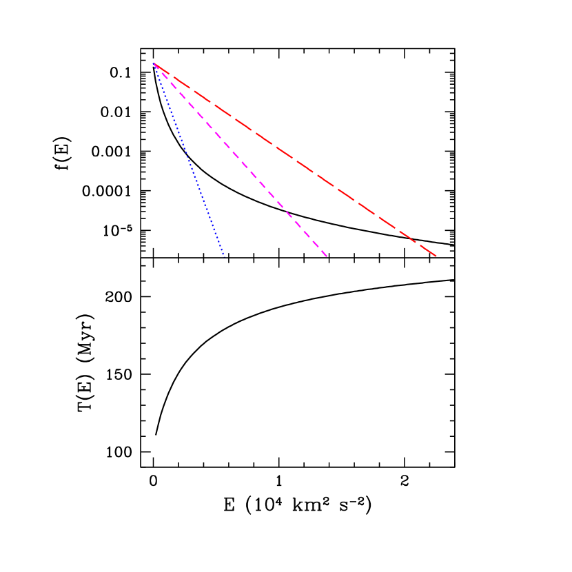
Figure 1: Phase space DFs and vertical oscillation period $T(E)$ for the equilibrium models described in Section 2.3. The upper panel shows the DFs for the disc stars (solid black), and tracer populations with $\sigma=20\,{\rm km\,s}^{-1}$ (dotted blue), $35\,{\rm km\,s}^{-1}$ (dashed magenta) and $50\,{\rm km\,s}^{-1}$ (long-dashed red). The normalization of the tracer DFs is arbitrary and for comparison purposes, we’ve set it to match that of the disc stars at $E=0$. The lower panel shows the vertical oscillation period as a function of energy.

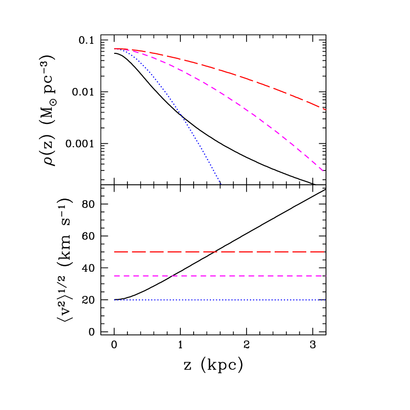
Figure 2: Density and vertical velocity dispersion as a function of $z$ for the equilibrium model described in Section 2.3. The upper panel shows the vertical density profile for the stars and the tracer subpopulations with $\sigma=20,\,35,\,50\,{\rm km\,s}^{-1}$. The lower panel shows the velocity dispersion. Line types and colours are the same as in Figure 1.

This form for the potential was introduced by Kuijken & Gilmore (1989a, b, c) in their series of papers on the Oort problem. We choose parameters to roughly match the stellar density in the solar neighborhood. In particular, we set $\rho_{\rm DM}=0.0114\,{\rm M}_{\odot}\,{\rm pc}^{-3}$, $\Sigma_{b}=48.4\,M_{\odot}\,\rm{pc}^{-2}$ and $h=0.435\,{\rm kpc}$, which yields a vertical density profile in good agreement with the vertical density profile from Jurić et al. (2008). Note that ratio of the contribution to the vertical force from the dark matter to that of the baryons from the stellar disc is $K_{DM}(z)/K_{b}(z)=\left(2\rho_{DM}h/\Sigma_{b}\right)\left(1+z^{2}/h^{2}\right)^{1/2}$, which implies that at $z=1.1\,{\rm kpc}$, the dark matter accounts for roughly $36\,\%$ of the total vertical force. Thus, a $10\,\%$ systematic error in $K_{1.1}$ would imply a $25\,\%$ error in the inferred dark matter density.

In Appendix A, we derive an analytic expression for the distribution function of isothermal tracers embedded in this zero order potential. Figure 1 shows the equilibrium DFs for the stellar component and for three of the tracer subpopulations. Note that while the tracer DFs decrease exponentially with $E$, the DF for the stellar disc decreases as a power-law with $E$ as $E\to\infty$, a result of the power-law decrease in the density profile at large $z$ (See Appendix A). Also shown is the vertical oscillation period, which increases from $\sim 100\,{\rm Myr}$ near to the midplane, to $200\,{\rm Myr}$ at $|z|\simeq 2\,{\rm kpc}$. Figure 2 shows the vertical density and velocity dispersion profiles for the three stellar systems. In principle, the disc stars could be represented as a superposition of isothermal populations.

We then assume that the DFs of the tracers and the stellar disc are perturbed as in Eq. 13, with $\epsilon=0.2$ and $\gamma=\pi/2$. With these choices $\langle z^{2}\rangle$ and $\langle v^{2}\rangle$ are initially equal to their equilibrium values while $\langle zv\rangle\simeq 2-5\,{\rm km\,s}^{-1}$. The latter is consistent with measurements of the bulk vertical velocities in the solar neighbourhood (Widrow et al., 2012; Williams et al., 2013; Carlin et al., 2013). This perturbation then feeds back into the potential of the stellar disc The system is evolved using an N-body code in which the disc stars and tracers are modeled as plane symmetric sheets (one-dimensional “particles”) that interact via gravity (see, for example, Weinberg (1991)). Gravity in a plane-symmetric system is particularly simple since the force on a given particle at position $z^{\prime}$ is proportional to the difference between the number of particles with $z>z^{\prime}$ and the number with $z<z^{\prime}$. Thus, forces at each timestep can be obtained by sorting the particles in $z$.

The stellar disc is modeled with $4\times 10^{5}$ particles. This number of particles is more than adequate for modeling one spatial and two phase space dimensions as test simulations with fewer disc particles confirm. For the tracers, we note that the stellar surface density at the position of the Sun is $\sim 50\,\rm{M_{\odot}\,pc^{-2}}$, which implies that a local patch of the disc $1\,{\rm kpc}$ across will contain some $10^{7}-10^{8}$ stars. The Gaia mission (Perryman et al., 2001; Lindegren et al., 2008) aims to provide kinematic data for a large fraction of these stars. One might then imagine dividing these stars into $O(100)$ subpopulations that are defined by chemical abundances as in Bovy & Rix (2013). Each of these subpopulations can then be used as an independent, isothermal tracer of the gravitational potential. With these numbers in mind, we model each of the tracer subpopulations with $10^{5}$ particles.

In Figure 3 we show the evolution of $\langle z^{2}\rangle$, $\langle v^{2}\rangle$, and $\langle zv\rangle$ in the presence of the perturbation. The general features of the oscillations are easy to understand. First, the vertical oscillations for the coldest tracers ($\sigma=20\,{\rm km\,s}^{-1}$) have a period $\sim 70\,{\rm Myr}$. As expected for an $m=2$ breathing mode, this is half the vertical oscillation period for a typical star in this subpopulation (see Figure 1). The oscillation periods for the $\sigma=35\,{\rm km\,s}^{-1}$ and $50\,{\rm km\,s}^{-1}$ subpopulations are somewhat longer, consistent with the fact that these populations are comprised of stars with higher vertical energies and therefore longer oscillation periods. The oscillations damp due to phase mixing and the damping is strongest for the coldest population where the dynamical time is shortest. We conclude that the amplitude and phase of vertical oscillations in different subpopulations need not be the same.

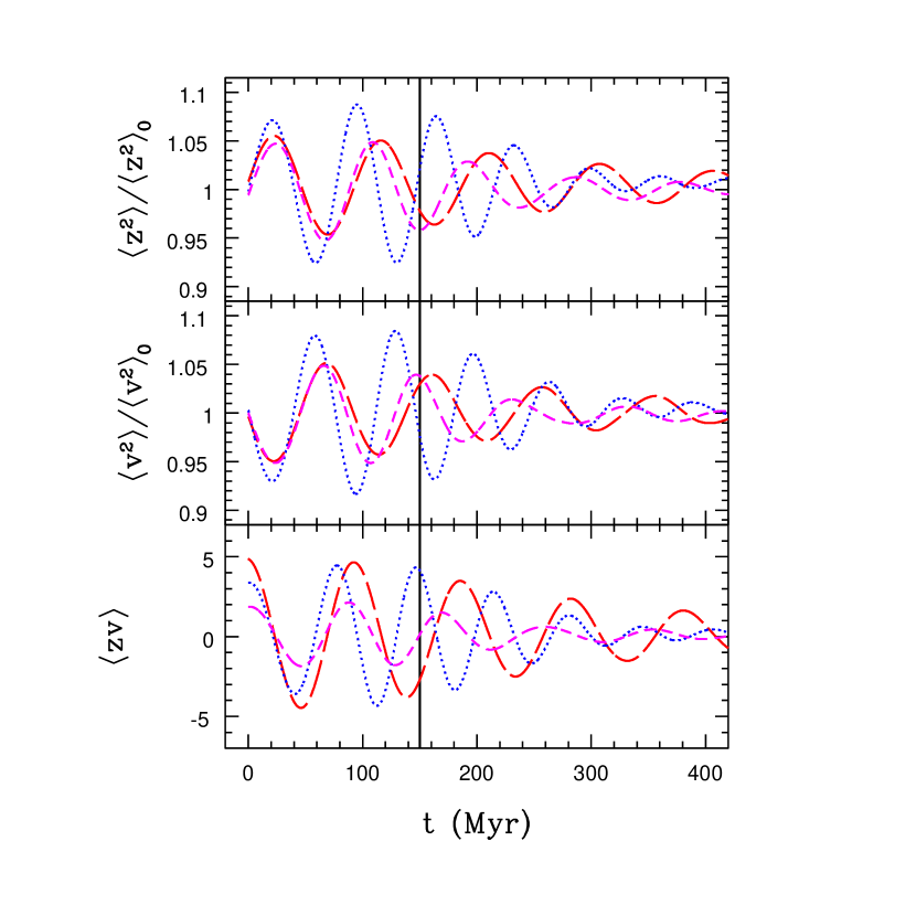
Figure 3: Time evolution of the variance in $z$ and $v$ as well as $\langle zv\rangle$ for three subpopulations. The top panel shows the variance in $z$ normalized to the equilibrium value for $\sigma=20,\,35,\,50\,{\rm km\,s}^{-1}$. Line types and colours are the same as in Figure 1. The middle panel shows the same for $v$. Bottom panel shows the time evolution of $\langle zv\rangle$ in units of ${\rm km\,s}^{-1}\,{\rm kpc}$. The vertical line here and in Figure 4 indicates the epoch at which we generate the mock catalogs that are analyzed in §3.

In Figure 4 we show the time evolution of the surface density within $1.1\,{\rm kpc}$ as well as an estimator for the vertical force $\langle v^{2}\rangle/\sqrt{\langle}z^{2}\rangle$. We see that the amplitude of the oscillations in the former are an order of magnitude smaller than those of the latter. Thus errors in estimates of the local vertical force that arise when the tracers are out of equilibrium are likely to be far more significant than oscillations in the force itself.

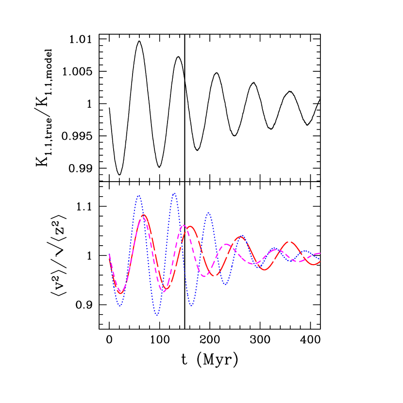
Figure 4: In the presence of a perturbation, the time evolution of the surface density (top) and an estimator for it, $\langle v^{2}\rangle/\sqrt{\langle z^{2}\rangle}$. The latter is an estimator for the vertical force. Both quantities have been normalized to their equilibrium values. Line types and colours are the same as in Figure 3.

3 parameter biases induced by non-equilibrium effects

In this section, we treat kinematic snapshots of the simulation described in §2.3 as mock data that can be analysed to infer the gravitational potential and force. The results are then compared with the equilibrium potential and force and the true (that is, perturbed) potential and force.

For a sample of $N$ tracers from a particular subpopulation, the assumed likelihood function is

$$\mathcal{L}\left(\rho_{\rm DM},h,\Sigma_{b},\sigma\right)=\prod_{i=1}^{N}\left[{\cal N}(\rho_{\rm DM},h,\Sigma_{b},\sigma)\,e^{-E_{i}/\sigma^{2}}\right]$$ (25)

where $E_{i}=v_{i}^{2}/2+\psi(z_{i})$ is the energy of the $i^{\rm{th}}$ star from the sample,$\psi$ is given by Eq. 24, and

$${\cal N}=\left(\int dz\,dv\exp{\left(-E/\sigma^{2}\right)}\right)^{-1}$$ (26)

is a normalization constant. We assume uniform priors in the model parameters $\rho_{\rm DM},h,\,\Sigma_{b}$ and $\sigma$ and sample the posterior probability distribution function (PDF) using EMCEE Foreman-Mackey et al. (2013), which implements the ensemble sampler of Goodman & Weare (2010).

Here we investigate the extent to which the equilibrium assumption will bias the parameters of the potentials, that is, the amount by which the parameters are mis-estimated when the true distribution has a non-equilibrium signature as described in §2.

Figure 5 shows the model PDFs that are inferred from two mock data sets for the $\sigma=35\,{\rm km\,s}^{-1}$ tracer subpopulation. The first data set is drawn from an equilibrium distribution while the second is drawn from the $150\,{\rm Myr}$ snapshot of the simulation. As expected, when the data is drawn from an equilibrium distribution, that is, when the model correctly describes the data, the analysis recovers the model parameters to within the calculated uncertainties. We note that there is a strong negative correlation between $\Sigma_{b}$ and $\rho_{\rm DM}$, which indicates a degeneracy in the disc and halo contributions to the potential. That is, the data are most sensitive to the total force and this can be kept close to fixed by increasing the dark matter density while decreasing $\Sigma_{b}$. The degeneracy between dark and visible matter was noted previously by Bahcall (1984a), Kuijken & Gilmore (1991), and Garbari et al. (2012) (see also Read 2014) and can be partially broken by extending the sample of stars with larger values of $z$. There is also a strong positive correlation between $\Sigma_{b}$ and $h$, which we might have anticipated by considering the leading term in the Taylor expansion of the disc contribution to the potential: $2\pi G\Sigma_{b}z^{2}/2h$.

The striking result in Figure 5 is that inferred value of the local dark matter density differs by a factor of two from the true value in the presence of this (quite realistic) breathing mode. Not surprisingly, when viewed in the $\Sigma_{b}-\rho_{\rm DM}$ and $\Sigma_{b}-h$ planes, these departures tend to lie along the degeneracies mentioned above. Thus, we expect that the inferrences in the vertical force or, alternatively, the total surface density will be more robust. This point was discussed in Kuijken & Gilmore (1991) and Figure 6 shows that it is indeed the case. In particular, when the $35\,{\rm km\,s}^{-1}$ tracers are perturbed, $K_{1.1}$ is over-estimated by only about $10\%$. With a sample size of $10^{5}$ stars and “perfect” data (we have made no attempt to model observational uncertainties) this systematic error still represents a $5$-sigma departure from the true value.

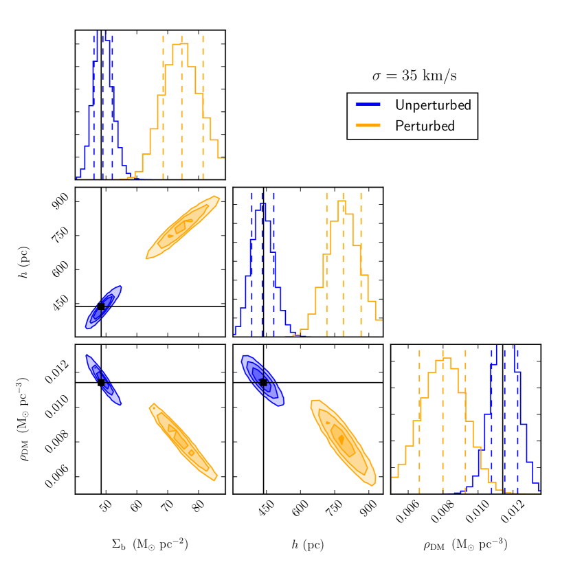
Figure 5: PDF in the model parameter space given two mock data sets that sample the $\sigma=35\,{\rm km\,s}^{-1}$ subpopulation. Each panel shows a different two-dimensional projection of the PDF in the parameter space defined by $\left(\Sigma_{b},\,h,\,\rho_{\rm DM},\,\sigma\right)$. Orange contours are for a sample drawn from the equilibrium distribution; blue contours are for a sample drawn from a distribution that has been perturbed by a breathing mode, namely the $150\,{\rm Myr}$ snapshot of the N-body simulation described in §2.3.

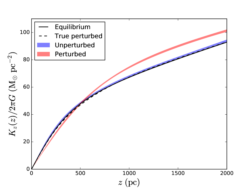
Figure 6: Magnitude of the vertical force $K_{z}(z)$ as inferred from the mock data sets described in §3.2 and used in Figure 5. Bands show the 68% confidence intervals for $K_{z}$ as a function of $z$. The blue band is for the equilibrium sample while the orange band is for the sample perturbed by a breathing mode. Also shown is the equilibrium vertical force (solid line) and true perturbed vertical force (dashed line).

4 From the Vertical Force to Disk Perturbations

It is an implicit assumption in the Oort problem that different tracer subpopulations will infer the same vertical force $K_{z}(z)$ to within the calculated uncertainties. This assumption is greatly exploited in the analysis of Bovy & Rix (2013) where dozens of MAPs are used as independent tracers of the gravitational potential. In this section we argue the converse: differences in the force inferred from different tracer subpopulations may provide evidence that the disc is in a perturbed state.

We begin by re-examining the results from Bovy & Rix (2013). Their analysis was based on a sample of 16K G dwarfs from SEGUE (Yanny et al., 2009) separated into 43 MAPs. For our purposes, each MAP can be distinguished by its vertical velocity dispersion $\sigma$ and a characteristic Galactocentric radius $R$. Our contention is that breathing mode perturbations may induce a dependence of $K_{z}$ on $\sigma$ for subpopulations at the same $R$ though as we’ll see, the precise nature of this dependence cannot be known a priori.

Bovy & Rix (2013) find that the MAPs with higher $\sigma$ tend to be closer to the Galactic centre. Furthermore, the vertical force at fixed $|z|$ decreases with increasing $R$. In particular Bovy & Rix (2013) find that vertical force at $|z|=1.1\,{\rm kpc}$ is well-fit by the exponential

$$\frac{K_{1.1}(R)}{2\pi G}=67\,M_{\odot}{\rm pc}^{-2}\exp{\left(-\left(R-R_{0}\right)/2.7\,{\rm kpc}\right)}$$ (27)

where $R_{0}=8\,{\rm kpc}$ is the distance of the Sun from the Galactic centre. Together, these results imply that there is an “accidental” correlation between $\sigma$ and $K_{1.1}$. To remove this correlation we correct $K_{1.1}$ using Eq. 27 so that each MAP provides an estimate of the vertical force at $R=R_{0}$. In addition, we separately consider estimates for $K_{1.1}$ from subpopulations that probe the potential within $1$ kpc bands in $R$. The results for $6\,{\rm kpc}<R<7\,{\rm kpc}$ and $7\,{\rm kpc}<R<8\,{\rm kpc}$ are shown in Figure 7. These results are consistent with the null hypothesis that $K_{1.1}$ is independent of $\sigma$ though there are hints of a trend toward systematically higher values of $K_{1.1}$ among the low-$\sigma$ subpopulations with $R$ between $6$ and $7$ kpc.

Figure 7: $K_{1.1}$ vs. $\sigma$ for different MAPs from the analysis of Bovy & Rix (2013). Left panel shows MAPs with characteristic radius in the range $6{\rm kpc}<R<7\,{\rm kpc}$ while the right panel is for the range $7\,{\rm kpc}<R<8\,{\rm kpc}$. Values of $K_{1.1}$ have been corrected to the position of the Sun using Eq. 27.

With only 100-800 stars in each MAP, the fractional uncertainties in $K_{1.1}$ found by Bovy & Rix (2013) are $10-20\%$ and therefore comparable to the anticipated effects of a breathing mode perturbation. Fortunately Gaia will increase the sample size by two or more orders of magnitude and therefore reduce the uncertainties by a factor of 10 or greater. With this in mind, we investigate whether the variations in $K_{z}$ with $\sigma$ that are induced by a breathing mode perturbation might be detected when the subpopulation sample size is $10^{5}$.

In Figure 8 we show PDFs for the model parameters that are inferred from the $\sigma=20\,{\rm km\,s}^{-1}$, $\sigma=35\,{\rm km\,s}^{-1}$ and $\sigma=50\,{\rm km\,s}^{-1}$ subpopulations. The mock data samples for these subpopulations are taken from the $150\,{\rm Myr}$ snapshot of the simulation. We see that the parameter determinations from the different tracers can disagree with one another at the multiple-sigma level (e.g., the ($h,\rho_{\rm DM}$) plane). This disagreement will provide a signal that the underlying model is incorrect. As in Figure 5, the confidence intervals from the different mock data sets tend to line up along the correlation ridges mentioned above. Nevertheless, there are departures off these ridges indicating that the different data sets will lead to slightly different estimates for $K_{z}$. Figure 9 shows the force inferred from each tracer. Although all the three inferences differ from the truth by  20%, they disagree with one another at only about the 5% level.

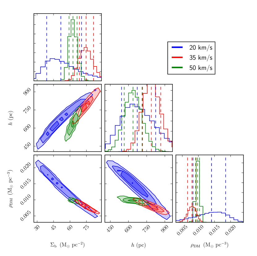
Figure 8: PDF for the model parameters as inferred from three different perturbed subpopulations. The mock data sets are from the $150\,{\rm Myr}$ snapshot of the simulation described in §2.3. Blue contours are from the $\sigma=20\,{\rm km\,s}^{-1}$ sample, red contours are from the $\sigma=35\,{\rm km\,s}^{-1}$ sample and therefore the same as the contours found in Figure 5 and green contours are from the $\sigma=50\,{\rm km\,s}^{-1}$ sample.

In Figure 10, we present a scatter plot of $\Sigma_{b}$ and $\rho_{\rm DM}$ as inferred from an analysis of mock data for eight subpopulations with $\sigma=20,25,30,35,40,45,50~{}\rm{and}~{}55\,{\rm km\,s}^{-1}$ at five different snapshots of our simulation. This figure can be compared with the lower left panels of Figure 5 and 8. Recall that the initial conditions were chosen so that $\langle z^{2}\rangle$ and $\langle v^{2}\rangle$ were equal to their equilibrium values. Therefore, it is not surprising that with the initial snapshot (solid black circles), the true model parameters are recovered quite accurately. For the later snapshots, when $\langle z^{2}\rangle$ and $\langle v^{2}\rangle$ depart from their equilibrium values, the different tracers can yield significantly different values for the model parameters. The results also vary significantly from snapshot to snapshot, a reflection of the stochastic nature of disc perturbations. The models do tend to lie along a narrow ridge in $K_{1.1}$ and this once again illustrates that it is the vertical force or total surface density that is most robustly determined from the stellar dynamics.

To further illustrate how $K_{z}$ might depend on $\sigma$ we show, in Figure 11, $K_{1.1}$ for the subpopulations and simulation snapshots used in Figure 10. Once again, for the initial conditions the model recovers the true value of $K_{1.1}$ to within the calculated uncertainties. Each of the other snapshots show a different example of what a $K_{1.1}$-$\sigma$ curve might look like. The model might systematically overestimate $K_{1.1}$, as with the $50$ and $150\,{\rm Myr}$ snapshots or underestimate $K_{1.1}$, as with the $100\,{\rm Myr}$ snapshot. Typical variations in $K_{1.1}$ across the range in $\sigma$ are $\sim 5\%$ though in one example, the $200\,{\rm Myr}$ snapshot the variation is greater than $10\%$.

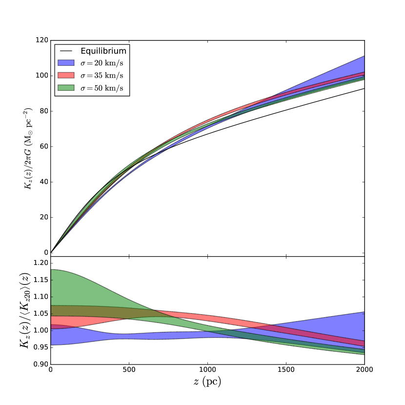
Figure 9: 68% confidence intervals for $K_{z}$ derived from the PDFs shown in Figure 8. In the lower panel, we show the confidence intervals for $K_{z}$ divided by the mean values for the $\sigma=20\,{\rm km\,s}^{-1}$ sample. Also shown as a solid black line is $K_{z}$ for the equilibrium potential.

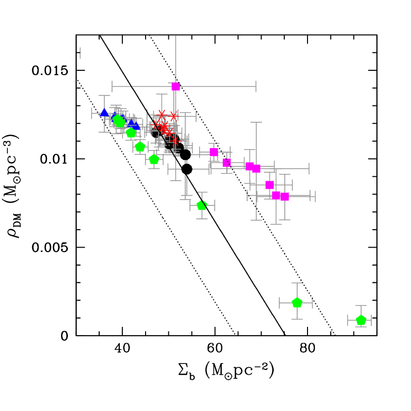
Figure 10: Estimates for $\Sigma_{b}$ and $\rho_{\rm DM}$ from eight subpopulations at five snapshots from the simulation described in §2.3. Initial conditions are shown as black circles. Other snapshots are shown as red stars, blue triangles, magenta squares, green pentagons for snapshots spaced at $50\,{\rm Myr}$ intervals.

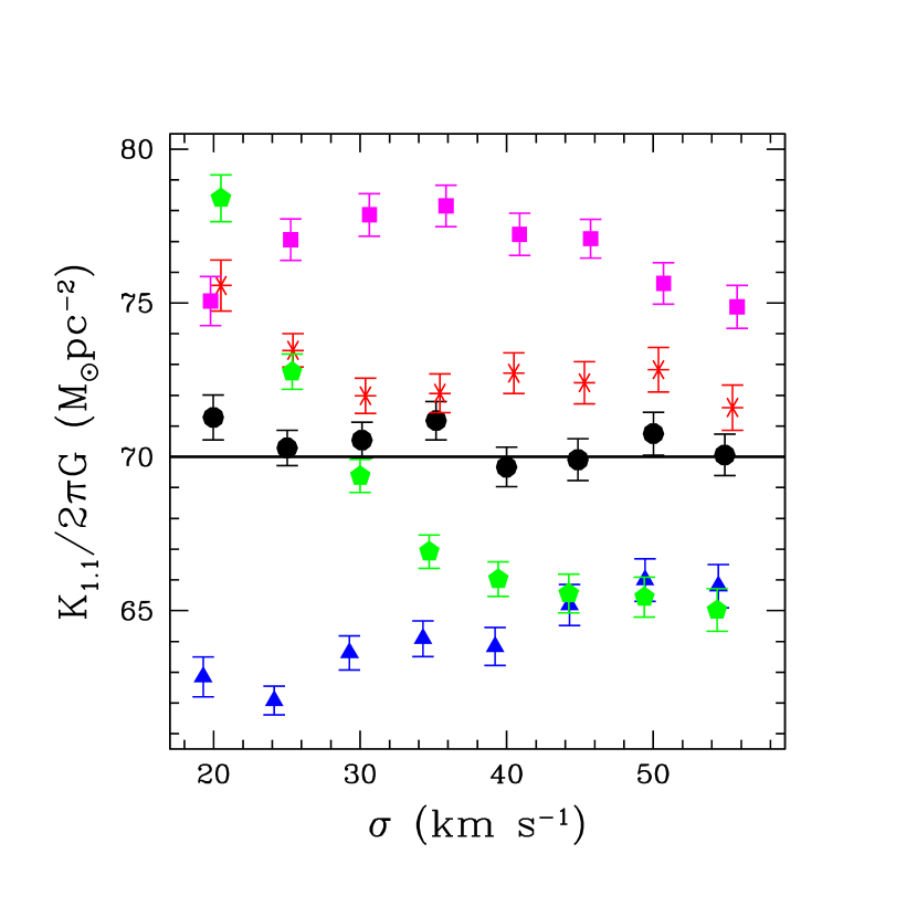
Figure 11: Estimates for $K_{1.1}$ as a function of $\sigma$ for eight subpopulations and five snapshots. Point types and colours are the same as in Figure 10.

5 Conclusions

The traditional Oort analysis assumes an underlying equilibrium distribution for stars in the solar neighbourhood. Perturbations in the potential, and indeed there is evidence already for a perturbation in the form of a breathing mode, can upset the inferences from these analyses. In the presence of this perturbation, a mismatch between the true and inferred values of the vertical force has important implications, especially as we enter the Gaia era, where observations of many different tracers, each with of order $10^{5}$ velocities and positions, are feasible. Here we have run mock observations to quantify the following three effects of a perturbed disc:

• The vertical force as inferred from a single tracer may differ from the true value by $10\%$ or greater, depending on the phase and amplitude of the perturbation. This error is distinct from other sources of statistical and systematic uncertainties inherent in the Oort problem. The corresponding error in an estimate of the local dark matter density would be at the $25\%$ level.

• An analysis of multiple tracers, each with different velocity dispersions, will lead to inconsistent conclusions about the total surface density profile thereby providing evidence that the underlying model – assumed to be equilibrium – was wrong. With enough tracers, one could imagine discovering something about the cause of the perturbation, be it a passing dark matter sub-halo or nearby dwarf galaxy or some other transient phenomena in the disc.

• Agreement among the conclusions from multiple tracers would improve the robustness of the dark matter determination: if all the tracers give the same answer, we can be confident that the underlying model and the conclusions inferred from it are correct.

  The main limitation of our analysis is that it treats the Galaxy as a plane-symmetric system. This simplification allowed us to focus on the effects of a perturbed disc. In the full three-dimensional Galaxy, additional complications might arise, which could masquerade as disc perturbations. For example, a tilt of the velocity ellipsoid away from the plane of the disc can bias estimates of the dark matter density if not properly modeled (see for example, Kuijken & Gilmore (1989a,b,c), Garbari et al. (2012), and more recently, Silverwood et al. (2016)). Of course, in a perturbed disc, the tilt might vary across the different MAPs and, in principle, could itself be a time-dependent feature of the perturbed disc. The promise of Gaia is that we will be able to disentangle these different effects and ultimately place robust constraints on the local density of dark matter.

Acknowledgments – The authors are grateful to Brian Yanny, Alex Drlica-Wagner, Elise Jennings, and Jo Bovy for useful comments and discussions. Fermilab is operated by Fermi Research Alliance, LLC, under Contract No. DE-AC02-07CH11359 with the U.S. Department of Energy. NB was supported by the Fermilab Graduate Student Research Program in Theoretical Physics. LMW was supported by a Discovery Grant with the Natural Sciences and Engineering Research Council of Canada.

6 Appendix

In this section, we derive the analytic DF for the baryon component introduced in Section 2.3. In general, the density for a plane-symmetric system is derived from the DF by the integral $\rho(z)=\int dvf(z,\,v)$. For an equilibrium system

$$\rho\left(\psi\right)=\frac{1}{\sqrt{2}}\int_{\psi}^{\infty}\frac{dEf(E)}{\sqrt{E-\psi}}$$ (28)

By an Abel transform, we have

$$f(E)=-\frac{1}{\sqrt{2}\pi}\int_{E}^{\infty}\frac{d\rho}{d\psi}\frac{d\psi}{\sqrt{\psi-E}}$$ (29)

It is convenient to write the potential and density in terms of $u\equiv\left(1+z^{2}/h^{2}\right)^{1/2}$:

$$\psi=2\pi G\left(\rho_{dm}h^{2}u^{2}+\Sigma_{b}hu-\Sigma_{b}h-\rho_{dm}h^{2}\right)$$ (30)

and

$$\rho_{b}=\frac{\Sigma_{b}}{2hu^{3}}~{}.$$ (31)

We then have

$$f(E) =\frac{3\Sigma_{b}}{\sqrt{8}\pi h}\int_{u(E)}^{\infty}\frac{du}{u^{4}\sqrt{\psi(u)-E}}$$ (32)

$$=\frac{3}{4\pi}\frac{\Sigma_{b}}{h}\frac{1}{\sqrt{\pi G\Sigma_{b}h}}\int_{u(E)}^{\infty}\frac{du}{u^{4}\left(\alpha u^{2}+u-\mathcal{E}\right)^{1/2}}$$ (33)

where $\alpha\equiv\rho_{dm}h/\Sigma_{b}$, $\mathcal{E}\equiv E/\left(2\pi G\Sigma_{b}h\right)+1+\alpha$ and $u(E)=\left(\left(1+4\alpha\mathcal{E}\right)^{1/2}-1\right)/2\alpha$. The integral can be expressed in terms of elementary functions are we have

$$f(E)=\frac{3}{4}\left(\frac{\Sigma_{b}}{\pi^{3}Gh^{3}}\right)^{1/2}\frac{1}{\mathcal{E}^{7/2}}\mathcal{F}\left(\left(\alpha\mathcal{E}\right)^{1/2}\right)$$ (34)

where

$$\mathcal{F}(x)=\frac{1}{96}\left(\left(72x^{2}+30\right){\rm ctn}^{-1}(2x)+15\pi+60x+36\pi x^{2}+64x^{3}\right)~{}.$$ (35)

References

- Bahcall (1984a) Bahcall, J. N. 1984, ApJ, 276, 169
- Bahcall (1984b) Bahcall, J. N. 1984, ApJ, 287, 926
- Bienayme et al. (1987) Bienayme, O., Robin, A. C., & Creze, M. 1987, A&A, 180, 94
- Binney (2010) Binney, J. 2010, MNRAS, 401, 2318
- Binney & McMillan (2011) Binney, J., & McMillan, P. 2011, MNRAS, 413, 1889
- Bovy & Rix (2013) Bovy, J., & Rix, H.-W. 2013, ApJ, 779, 115
- Bovy & Tremaine (2012) Bovy, J., & Tremaine, S. 2012, ApJ, 756, 89
- Carlin et al. (2013) Carlin, J. L., DeLaunay, J., Newberg, H. J., et al. 2013, ApJL, 777, L5
- Debattista (2014) Debattista, V. P. 2014, MNRAS, 443, L1
- Faure et al. (2014) Faure, C., Siebert, A., & Famaey, B. 2014, MNRAS, 440, 2564
- Feldmann & Spolyar (2015) Feldmann, R., & Spolyar, D. 2015, MNRAS, 446, 1000
- Foreman-Mackey et al. (2013) Foreman-Mackey, D., Hogg, D. W., Lang, D., & Goodman, J. 2013, PASP, 125, 306
- Garbari et al. (2011) Garbari, S., Read, J. I., & Lake, G. 2011, MNRAS, 416, 2318
- Garbari et al. (2012) Garbari, S., Liu, C., Read, J. I., & Lake, G. 2012, MNRAS, 425, 1445
- Gómez et al. (2013) Gómez, F. A., Minchev, I., O’Shea, B. W., et al. 2013, MNRAS, 429, 159
- Goodman & Weare (2010) Goodman, J., & Weare, J. 2010, Commun. Appl. Math. Comput. Sci. 5, 65
- Holmberg & Flynn (2000) Holmberg, J., & Flynn, C. 2000, MNRAS, 313, 209
- Holmberg & Flynn (2004) Holmberg, J., & Flynn, C. 2004, MNRAS, 352, 440
- Jurić et al. (2008) Jurić, M., Ivezić, Ž., Brooks, A., et al. 2008, ApJ, 673, 864-914
- Kapteyn (1922) Kapteyn, J. C. 1922, ApJ, 55, 302
- Kuijken & Gilmore (1989a) Kuijken, K., & Gilmore, G. 1989, MNRAS, 239, 571
- Kuijken & Gilmore (1989b) Kuijken, K., & Gilmore, G. 1989, MNRAS, 239, 605
- Kuijken & Gilmore (1989c) Kuijken, K., & Gilmore, G. 1989, MNRAS, 239, 651
- Kuijken & Gilmore (1991) Kuijken, K., & Gilmore, G. 1991, ApJL, 367, L9
- Lindegren et al. (2008) Lindegren, L., Babusiaux, C., Bailer-Jones, C., et al. 2008, A Giant Step: from Milli- to Micro-arcsecond Astrometry, 248, 217
- Mathur (1990) Mathur, S. D. 1990, MNRAS, 243, 529
- Oort (1932) Oort, J. H. 1932, Bull. Astron. Inst. Neth., 6, 249
- Perryman et al. (2001) Perryman, M. A. C., de Boer, K. S., Gilmore, G., et al. 2001, A&A, 369, 339
- Read (2014) Read, J. I. 2014, Journal of Physics G Nuclear Physics, 41, 063101
- Silverwood et al. (2016) Silverwood, H., Sivertsson, S., Steger, P., Read, J. I., & Bertone, G. 2016, MNRAS, 459, 4191
- Ting et al. (2013) Ting, Y.-S., Rix, H.-W., Bovy, J., & van de Ven, G. 2013, MNRAS, 434, 652
- Weinberg (1991) Weinberg, M. D. 1991, ApJ, 373, 391
- Widrow et al. (2012) Widrow, L. M., Gardner, S., Yanny, B., Dodelson, S., & Chen, H.-Y. 2012, ApJL, 750, L41
- Widrow & Bonner (2015) Widrow, L. M., & Bonner, G. 2015, MNRAS, 450, 266
- Widrow et al. (2014) Widrow, L. M., Barber, J., Chequers, M. H., & Cheng, E. 2014, MNRAS, 440, 1971
- Williams et al. (2013) Williams, M. E. K., Steinmetz, M., Binney, J., et al. 2013, MNRAS, 436, 101
- Xu et al. (2015) Xu, Y., Newberg, H. J., Carlin, J. L., et al. 2015, ApJ, 801, 105
- Yanny et al. (2009) Yanny, B., Rockosi, C., Newberg, H. J., et al. 2009, AJ, 137, 4377-4399
- Yanny & Gardner (2013) Yanny, B., & Gardner, S. 2013, ApJ, 777, 91