Architecture Diagrams: A Graphical Language for Architecture Style Specification

Abstract

Architecture styles characterise families of architectures sharing common characteristics. We have recently proposed configuration logics for architecture style specification. In this paper, we study a graphical notation to enhance readability and easiness of expression. We study simple architecture diagrams and a more expressive extension, interval architecture diagrams. For each type of diagrams, we present its semantics, a set of necessary and sufficient consistency conditions and a method that allows to characterise compositionally the specified architectures. We provide several examples illustrating the application of the results. We also present a polynomial-time algorithm for checking that a given architecture conforms to the architecture style specified by a diagram.

1 Introduction

Software architectures [perry1992foundations, shaw1996software] describe the high-level structure of a system in terms of components and component interactions. They depict generic coordination principles between types of components and can be considered as generic operators that take as argument a set of components to be coordinated and return a composite component that satisfies by construction a given characteristic property [AttieBBJS15-architectures-faoc].

Many languages have been proposed for architecture description, such as architecture description languages (e.g. [medvidovic2000classification, iso2011]), coordination languages (e.g. [Papadopoulos1998329, reo]) and configuration languages (e.g. [wermelinger2001graph, kramer1990configuration]). All these works rely on the distinction between behaviour of individual components and their coordination in the overall system organization. Informally, architectures are characterized by the structure of the interactions between a set of typed components. The structure is usually specified as a relation, e.g. connectors between component ports.

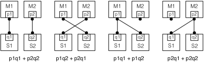
Figure 1: Master/Slave architectures.

Architecture styles characterise not a single architecture but a family of architectures sharing common characteristics, such as the types of the involved components and the topology induced by their coordination structure. Simple examples of architecture styles are Pipeline, Ring, Master/Slave, Pipes and Filters. For instance, Master/Slave architectures integrate two types of components, masters and slaves, such that each slave can interact only with one master. Fig. 1 depicts four Master/Slave architectures involving two master components $M_{1}$, $M_{2}$ and two slave components $S_{1}$, $S_{2}$. Their communication ports are respectively $p_{1}$, $p_{2}$ and $q_{1}$, $q_{2}$. A Master/Slave architecture for two masters and two slaves can be represented as one among the following configurations, i.e. sets of connectors: $\{p_{1}q_{1},p_{2}q_{2}\}$, $\{p_{1}q_{2},p_{2}q_{1}\}$, $\{p_{1}q_{1},p_{1}q_{2}\}$, $\{p_{2}q_{1},p_{2}q_{2}\}$. A term $p_{i}q_{j}$ represents a connector between ports $p_{i}$ and $q_{j}$. The four architectures are depicted in Fig. 1. The Master/Slave architecture style denotes all the Master/Slave architectures for arbitrary numbers of masters and slaves.

We have recently proposed configuration logics [cl-mas] for the description of architecture styles. These are powerset extensions of interaction logics [algconn] used to describe architectures. In addition to the operators of the extended logic, they have logical operators on sets of architectures. We have studied higher-order configuration logics and shown that they are a powerful tool for architecture style specification. Nonetheless, their richness in operators and concepts may make their use challenging.

In this paper we explore a different avenue to architecture style specification based on architecture diagrams. Architecture diagrams describe the structure of a system by showing the system’s component types and their attributes for coordination, as well as relationships among component types. Our notation allows the specification of generic coordination mechanisms based on the concept of connector.

Architecture diagrams were mainly developed for architecture style specification in BIP [AttieBBJS15-architectures-faoc], where connectors are defined as $n$-ary synchronizations among component ports and do not carry any additional behaviour. Nevertheless, our approach can be extended for architecture style specification in other languages by explicitly associating the required behaviour to connectors.

An architecture diagram consists of a set of component types, a cardinality function and a set of connector motifs. Component types are characterised by sets of generic ports. The cardinality function associates each component type with its cardinality, i.e. number of instances. Fig. 3 shows an architecture diagram consisting of three component types $T_{1}$, $T_{2}$ and $T_{3}$ with $n_{1}$, $n_{2}$ and $n_{3}$ instances and generic ports $p$, $q$ and $r$, respectively. Instantiated components have port instances $p_{i}$, $q_{j}$, $r_{k}$ for $i,j,k$ belonging to the intervals $[1,n_{1}]$, $[1,n_{2}]$, $[1,n_{3}]$, respectively.

Connector motifs are non-empty sets of generic ports that must interact. Each generic port $p$ in the connector motif has two constraints represented as a pair $m:d$. Multiplicity $m$ is the number of port instances $p_{i}$ that are involved in each connector. Degree $d$ specifies the number of connectors in which each port instance is involved. The architecture diagram of Fig. 3 has a single connector motif involving generic ports $p$, $q$ and $r$.

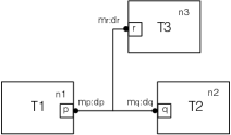
Figure 2: An architecture diagram.

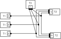
Figure 3: An architecture.

A connector motif defines a set of possible configurations, where a configuration is a set of connectors. The meaning of an architecture diagram is a set of architectures that contain the union of all sub-configurations corresponding to each connector motif of the diagram. Fig. 3 shows the unique architecture obtained from the diagram of Fig. 3 by taking $n_{1}=3$, $m_{p}=1$, $d_{p}=1$; $n_{2}=2$, $m_{q}=2$, $d_{q}=3$, $n_{3}=1$, $m_{r}=1$, $d_{r}=3$. This is the result of composition of constraints for generic ports $p$, $q$ and $r$. For $p$, we have three instances and as both the multiplicity and the degree are equal to $1$, each instance $p_{i}$ has a single connector lead. For $q$, we have two instances and as the multiplicity is $2$, we have connectors involving $q_{1}$ and $q_{2}$ and their total number is equal to $3$ to meet the degree constraint. For $r$, we have a single instance $r_{1}$ that has three connector leads to satisfy the degree constraint.

We study a method that allows to characterise compositionally the set of configurations specified by a given connector motif if consistency conditions are met. It involves a two-step process. The first step consists in characterising configuration sets meeting the coordination constraints for each generic port $p$ of the connector motif. In the second step, connectors from the sets obtained from step one are fused one by one, so that the multiplicities and the degrees of the ports are preserved, to generate the configuration of the connector motif.

We study two types of architecture diagrams: simple architecture diagrams and interval architecture diagrams. In the former the cardinality, multiplicity and degree constraints are positive integers, while in the latter they can also be intervals. Interval diagrams are strictly more expressive than simple diagrams. For each type of diagrams we present 1) its syntax and semantics; 2) a set of consistency conditions; 3) a method that allows to characterise compositionally all configurations of a connector motif; 4) examples of architecture style specification. Finally, we present a polynomial-time algorithm for checking that a given diagram conforms to the architecture style specified by a diagram.

A complete presentation, with proofs and additional examples, of the results in this paper can be found in the technical report [MBBS16-Diagrams-TR].

The paper is structured as follows. Sects. 2 and 3 present simple and interval architecture diagrams, respectively. Sect. 4 presents an algorithm for checking conformance of diagrams. Sect. LABEL:sec:relatedwork discusses related work. Sect. LABEL:sec:discussion summarises the results and discusses possible directions for future work.

2 Simple Architecture Diagrams

2.1 Syntax and Semantics

We focus on the specification of generic coordination mechanisms based on the concept of connector. Therefore, the nature and the operational semantics of components are irrelevant. As in the previous section, we consider that a component interface is defined by its set of ports, which are used for interaction with other components. Thus, a component type $T$ has a set of generic ports $T.P$.

A simple architecture diagram $\langle\mathcal{T},n,\mathcal{C}\rangle$ consists of: 1) a set of component types $\mathcal{T}=\{T_{1},\dots,T_{k}\}$; 2) an associated cardinality function $n:\mathcal{T}\rightarrow\mathbb{N}$, where $\mathbb{N}$ is the set of natural numbers (to simplify the notation, we will abbreviate $n(T_{i})$ to $n_{i}$); 3) a set of connector motifs $\mathcal{C}=\{\Gamma_{1},\dots,\Gamma_{l}\}$ of the form $\Gamma=(a,\{m_{p}:d_{p}\}_{p\in a})$, where $\emptyset\neq a\subseteq\bigcup_{i=1}^{k}T_{i}.P$ is a generic connector and $m_{p},d_{p}\in\mathbb{N}$ (with $m_{p}>0$) are the multiplicity and degree associated to generic port $p\in a$.

Fig. 4 shows the graphical representation of a simple architecture diagram with a connector motif.

Figure 4: A simple architecture diagram.

An architecture is a pair $\langle\mathcal{B},\gamma\rangle$, where $\mathcal{B}$ is a set of components and $\gamma$ is a configuration, i.e. a set of connectors among the ports of components in $\mathcal{B}$. We define a connector as a set of ports that must interact. For a component $B\in\mathcal{B}$ and a component type $T$, we say that $B$ is of type $T$ if the ports of $B$ are in a bijective correspondence with the generic ports in $T$. Let $B_{1},\dots,B_{n}$ be all the components of type $T$ in $\mathcal{B}$. For a generic port $p\in T.P$, we denote the corresponding port instances by $p_{1},\dots,p_{n}$ and its associated cardinality by $n_{p}=n(T)$.

Semantics 1.

An architecture $\langle\mathcal{B},\gamma\rangle$ conforms to a diagram $\langle\mathcal{T},n,\mathcal{C}\rangle$ if, for each $i\in[1,k]$, the number of components of type $T_{i}$ in $\mathcal{B}$ is equal to $n_{i}$ and $\gamma$ can be partitioned into disjoint sets $\gamma_{1},\dots,\gamma_{l}$, such that, for each connector motif $\Gamma_{j}=(a,\{m_{p}:d_{p}\}_{p\in a})\in\mathcal{C}$ and each $p\in a$, 1) there are exactly $m_{p}$ instances of $p$ in each connector in $\gamma_{j}$ and 2) each instance of $p$ is involved in exactly $d_{p}$ connectors in $\gamma_{j}$.

We assume that, for any two connector motifs $\Gamma_{i}=(a,\{m_{p}^{i}:d_{p}^{i}\}_{p\in a})$ (for $i=1,2$) with the same set of generic ports $a$, there exists $p\in a$, such that $m_{p}^{1}\neq m_{p}^{2}$. Without significant impact on the expressiveness of the formalism, this assumption simplifies semantics and analysis. Details are provided in [MBBS16-Diagrams-TR].

Multiplicity constrains the number of instances of the generic port that must participate in a connector, whereas degree constrains the number of connectors attached to any instance of the generic port. Consider the two diagrams and their conforming architectures shown in Figs. 6 and 6. They have the same set of component types and cardinalities. Nevertheless, their multiplicities and degrees differ, resulting in different architectures.

In Fig. 6, the multiplicity of generic port $p$ is $1$ and the multiplicity of generic port $q$ is $3$, thus, any connector must involve one instance of $p$ and all three instances of $q$. The degree of both generic ports is $1$, so each port instance is involved in exactly one connector. Thus, the diagram defines an architecture with one quaternary connector.

In Fig. 6 the multiplicities of both generic ports $p$ and $q$ are $1$. Thus, all connectors are binary and involve one instance of $p$ and one instance of $q$. The degree of $p$ is 3, thus three connectors are attached to each instance. Thus, the diagram defines an architecture with three binary connectors.

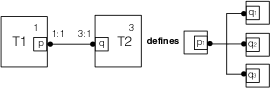
Figure 5: 4-ary synchronisation.

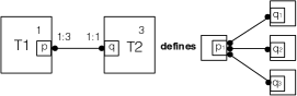
Figure 6: Binary synchronisation.

2.2 Consistency Conditions

Notice that there exist diagrams that do not define any architecture. Let us consider the diagram shown in Fig. 4 with $n_{1}=3$, $m_{p}=1$, $d_{p}=1$, $n_{2}=2$, $m_{q}=1$ and $d_{q}=1$. Since the multiplicity is $1$ for both generic ports $p$ and $q$, a conforming architecture must include only binary connectors involving one instance of $p$ and one instance of $q$. Since the degree of both $p$ and $q$ is $1$, each port instance must be involved in exactly one connector. However, the cardinalities impose that there be three connectors attached to the instances of $p$, but only two connectors attached to the instances of $q$. Both requirements cannot be satisfied simultaneously and thus, no architecture can conform to this diagram.

Consider a connector motif $\Gamma=(a,\{m_{p}:d_{p}\}_{p\in a})$ in a diagram $\langle\mathcal{T},n,\mathcal{C}\rangle$ and a generic port $p\in a$, such that $p\in T.P$, for some $T\in\mathcal{T}$. We denote $s_{p}=n_{p}\cdot d_{p}/m_{p}$ the matching factor of $p$.

A regular configuration of $p$ is a multiset of connectors, such that 1) each connector involves $m_{p}$ instances of $p$ and no other ports and 2) each of the $n_{p}$ instances of port $p$ is involved in exactly $d_{p}$ connectors. Notice the difference between a configuration and a regular configuration of $p$: the former defines a set of connectors, while the latter defines a multiset of sub-connectors involving only instances of generic port $p$. Considering the diagram in Fig. 3 and the architecture in Fig. 3 the only regular configuration of $r$ is the multiset $\{r_{1},\ r_{1},\ r_{1}\}$. The three copies of the singleton sub-connector $r_{1}$ are then fused with sub-connectors $p_{i}q_{1}q_{2}$ ($i=1,2,3$), resulting in a configuration with three distinct connectors.

Lemma 2.1.

Each regular configuration of a port $p$ has exactly $s_{p}$ connectors.

Prop. 2.2 provides the necessary and sufficient conditions for a simple architecture diagram to be consistent, i.e. to have at least one conforming architecture. The multiplicity of a generic port must not exceed the number of component instances that contain this port. The matching factors of all ports participating in the same connector motif must be equal integers. Finally, since the number of distinct connectors of a connector motif is bounded and equal to $\prod_{q\in a}{\binom{n_{q}}{m_{q}}}$, there must be enough connectors to build a configuration. Since, by the semantics of diagrams, connector motifs correspond to disjoint sets of connectors, these conditions are applied separately to each connector motif.

Proposition 2.2.

A simple architecture diagram has a conforming architecture iff, for each connector motif $\Gamma=(a,\{m_{p}:d_{p}\}_{p\in a})$ and each $p\in a$, we have: 1) $m_{p}\leq n_{p}$; 2) $\forall q\in a,\ s_{p}=s_{q}\in\mathbb{N}$ and 3) $s_{p}\leq\prod_{q\in a}{\binom{n_{q}}{m_{q}}}$.

2.3 Synthesis of Configurations

The synthesis procedure for each connector motif has the following two steps: 1) we find regular configurations for each generic port; 2) we fuse these regular configurations generating global configurations specified by the connector motif.

2.3.1 Regular Configurations of a Generic Port

We start with an example illustrating the first step of the synthesis procedure for a port $p$.

Example 1.

Consider a port $p$ with $n_{p}=4$ and $m_{p}=2$. There are $6$ connectors of multiplicity $2$: $p_{1}p_{2}$, $p_{1}p_{3}$, $p_{1}p_{4}$, $p_{2}p_{3}$, $p_{2}p_{4}$, $p_{3}p_{4}$, which correspond to the set of edges of a complete graph with vertices $p_{1}$, $p_{2}$, $p_{3}$, $p_{4}$. The regular configurations of $p$ for $d_{p}=1,2,3$, where each edge appears at most once are shown in Fig. 7.

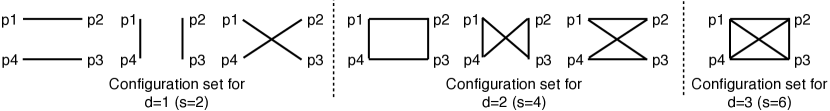
Figure 7: Regular configurations of $p$ with $n_{p}=4$, $m_{p}=2$.

We provide an equational characterisation of all the regular configurations (i.e. multisets of connectors) of a generic port $p$. Given $n_{p}$, $m_{p}$, $d_{p}$, for port instances $p_{1},\dots,p_{n_{p}}$, we associate a column vector of non-negative integer variables $X=[x_{1},\dots,x_{w}]^{T}$ to the set $\{a_{i}\}_{i\in[1,w]}$ of different connectors, where $w=\binom{n_{p}}{m_{p}}$.

Consider Ex. 1 and variables $x_{1},\dots,x_{6}$ representing the number of occurrences in a regular configuration of the connectors $p_{1}p_{2},\,p_{1}p_{3},\,p_{1}p_{4},\,p_{2}p_{3},\,p_{2}p_{4},\,$ $p_{3}p_{4}$, respectively. All the regular configurations, for $d_{p}=1,2,3$, represented as vectors of the form $[x_{1},\dots,x_{6}]$ are listed in Table 1. Notice that vectors for $d_{p}>1$ can be obtained as linear combinations of the vectors for $d_{p}=1$.

Table 1: Vector representation of regular configurations.

$\begin{array}[]{c|cc|cccc}\hline\cr d_{p}=1&\lx@intercol\hfil d_{p}=2\hfil\lx@intercol\vrule\lx@intercol&\lx@intercol\hfil d_{p}=3\hfil\lx@intercol\\ \hline\cr[100001]&[110011]&[200002]&[111111]&[120021]&[210012]&[300003]\\ {}[010010]&[101101]&[020020]&&[012210]&[021120]&[030030]\\ {}[001100]&[011110]&[002200]&&[102201]&[201102]&[003300]\\ \hline\cr\end{array}$

For $p$, we define an $n_{p}\times w$ incidence matrix $G=[g_{i,j}]_{n_{p}\times w}$ with $g_{i,j}=1$ if $p_{i}\in a_{j}$ and $g_{i,j}=0$ otherwise. We have $GX=D$, where $D=[d_{p},\dots,d_{p}]$ ($d_{p}$ repeated $n_{p}$ times). Any non-negative integer solution of this equation defines a regular configuration of $p$. For Ex. 1, the equations are:

$$\begin{cases}x_{1}+x_{2}+x_{3}=d_{p}\,,\\ x_{1}+x_{4}+x_{5}=d_{p}\,,\\ x_{2}+x_{4}+x_{6}=d_{p}\,,\\ x_{3}+x_{5}+x_{6}=d_{p}\,,\end{cases}\text{which is equivalent to\quad}\begin{cases}x_{1}+x_{2}+x_{3}=d_{p}\,,\\ x_{3}=x_{4}\,,\\ x_{2}=x_{5}\,,\\ x_{1}=x_{6}\,.\end{cases}$$ (1)

Notice that the vectors of Table 1 are solutions of (1).

2.3.2 Configurations of a Connector Motif

Let $\Gamma=(a,\{m_{p}:d_{p}\}_{p\in a})$ be a connector motif such that all generic ports of $a=\{p^{1},\dots,p^{v}\}$ have the same integer matching factor $s$. For each $p^{j}\in a$, let $\gamma^{j}=\{a_{i}^{j}\}_{i\in[1,s]}$ be a regular configuration of $p^{j}$. For arbitrary permutations $\pi_{j}$ of $[1,s]$, a set $\{a_{i}^{1}\cup\bigcup_{j=2}^{v}a_{\pi_{j}(i)}^{j}\}_{i\in[1,s]}$ is a configuration specified by the connector motif.

In order to provide an equational characterisation of the connector motif, we consider, for each $j\in[1,v]$, a corresponding solution vector $X^{j}$ of equations $G^{j}X^{j}=D^{j}$ characterising the regular configurations of $p^{j}$. We denote by $w^{j}$ the dimension of the vector $X^{j}$.

In order to characterise the configurations of connectors conforming to $\Gamma$, we consider, for each configuration, the $v$-dimensional matrix $E=[e_{i_{1},\dots,i_{v}}]_{w^{1}\times\dots\times w^{v}}$ of 0-1 variables, such that $e_{i_{1},\dots,i_{v}}=1$ if the connector $a_{i_{1}}^{1}\cup\dots\cup a_{i_{v}}^{v}$ belongs to the configuration and $0$ otherwise. By definition, the sum of all elements in $E$ is equal to $s$. Moreover, the following equations hold:

$$\left\{\begin{array}[]{r@{\ }c@{\ }ll}x_{i}^{1}&=&\Sigma_{i_{2},i_{3}\dots,i_{v}}\ e_{i,i_{2},\dots,i_{v}}\,,&\text{for $i\in[1,w^{1}]$,}\\ x_{i}^{2}&=&\Sigma_{i_{1},i_{3},\dots,i_{v}}\ e_{i_{1},i,\dots,i_{v}}\,,&\text{for $i\in[1,w^{2}]$,}\\ &\vdots\\ x_{i}^{v}&=&\Sigma_{i_{1},i_{2},\dots,i_{v-1}}\ e_{i_{1},\dots,i_{v-1},i}\,,&\text{for $i\in[1,w^{v}]$.}\end{array}\right.$$ (2)

For instance, for a fixed $i\in[1,w^{1}]$, $e_{i,i_{2},\dots,i_{v}}$ describe all connectors that contain $a_{i}^{1}$. The regular configuration $\gamma^{1}$ is characterised by $X^{1}$, enforcing that $a_{i}^{1}$ belongs to $x_{i}^{1}$ connectors. The set of linear equations (2), combined with the sets of linear equations $G^{j}X^{j}=D^{j}$, for $j\in[1,v]$, fully characterises the configurations of $\Gamma$ and can be used to synthesise architectures from architecture diagrams.

Example 2.

Consider a diagram $\bigl{(}\{T_{1},T_{2}\},n,\{\Gamma\}\bigr{)}$, where $T_{1}=\{p\}$, $T_{2}=\{q\}$, $n(T_{1})=n(T_{2})=4$ and $\Gamma=(pq,\{(m_{p}:d_{p},m_{q}:d_{q})\})$ with $m_{p}=2$, $m_{q}=3$. The corresponding equations $G_{p}X=D_{p}$, $G_{q}Y=D_{q}$ can be rewritten as

$$\begin{cases}x_{1}+x_{2}+x_{3}=d_{p},\\ x_{3}=x_{4},\ x_{2}=x_{5},\ x_{1}=x_{6},\ \end{cases}\text{and\quad}\begin{cases}3y_{1}=d_{q},\\ y_{1}=y_{2}=y_{3}=y_{4}.\end{cases}$$ (3)

Together with the constraints $x_{i}=\Sigma_{j}e_{i,j}$ and $y_{j}=\Sigma_{i}e_{i,j}$, for $E=[e_{i,j}]_{6\times 4}$, equations (3) completely characterise all the configurations conforming to $\Gamma$.

The same methodology can be used to synthesise configurations with additional constraints. To impose that some specific connectors must be included, whereas other specific connectors must be excluded from the configurations, the corresponding variables in the matrix $E$ are given fixed values: 1 (resp. 0) if the connector must be included (resp. excluded) from the configurations. The rest of the synthesis procedure remains the same.

Example 3.

Let us consider the diagram shown in Fig. 4 with $n_{1}=4$, $m_{p}=2$, $d_{p}=2$, $n_{2}=4$, $m_{q}=3$ and $d_{q}=3$. We want to synthesise the configurations of this diagram with the following additional constraints: connectors $p_{1}p_{2}q_{1}q_{2}q_{3}$ and $p_{1}p_{3}q_{2}q_{3}q_{4}$ must be included, whereas connector $p_{2}p_{4}q_{1}q_{2}q_{4}$ must be excluded.

First, we compute the vectors $X$ and $Y$ that represent the regular configurations of generic ports $p$ and $q$, respectively. Variables $x_{1},\dots,x_{6}$ represent the number of occurrences in a configuration of the connectors $p_{1}p_{2}$, $p_{1}p_{3}$, $p_{1}p_{4}$, $p_{2}p_{3}$, $p_{2}p_{4}$, $p_{3}p_{4}$, respectively. Variables $y_{1},\dots,y_{4}$ represent the number of occurrences in a configuration of the connectors $q_{1}q_{2}q_{3}$, $q_{1}q_{2}q_{4}$, $q_{1}q_{3}q_{4}$, $q_{2}q_{3}q_{4}$, respectively.

Vector $X$ can take one of the following values for $d_{p}=2$: $[110011]$, $[101101]$, $[011110]$, $[200002]$, $[020020]$ or $[002200]$ (Ex. 1). Regular configurations of $q$ are characterised by the equations $3y_{1}=d$ and $y_{1}=y_{2}=y_{3}=y_{4}$ (Ex. 2). For $d=3$ there is a single solution $Y=[1111]$.

We now consider the matrix $E$, where we fix $e_{1,1}=e_{2,4}=1$ and $e_{5,2}=0$ to impose the additional synthesis constraints as shown in Fig. 9. Since, for all $i\in[1,6]$, we have $x_{i}=\Sigma_{j}\,e_{i,j}$ and, for all $j\in[1,4]$, we have $y_{j}=\Sigma_{i}\,e_{i,j}$, we can deduce that the only possible valuation for $X$, $Y$ and $E$ is the one shown in Fig. 9 corresponding to configuration $\{p_{1}p_{2}q_{1}q_{2}q_{3},\ p_{1}p_{3}q_{2}q_{3}q_{4},\ p_{2}p_{4}q_{1}q_{3}q_{4},\ p_{3}p_{4}q_{1}q_{2}q_{4}\}.$

$$E=\bordermatrix{~{}&y_{1}&y_{2}&y_{3}&y_{4}\cr x_{1}&1&e_{1,2}&e_{1,3}&e_{1,4}\cr x_{2}&e_{2,1}&e_{2,2}&e_{2,3}&1\cr x_{3}&e_{3,1}&e_{3,2}&e_{3,3}&e_{3,4}\cr x_{4}&e_{4,1}&e_{4,2}&e_{4,3}&e_{4,4}\cr x_{5}&e_{5,1}&0&e_{5,3}&e_{5,4}\cr x_{6}&e_{6,1}&e_{6,2}&e_{6,3}&e_{6,4}\cr}$$

Figure 8: Matrix $E$ with fixed values.

$$E\quad=\quad\bordermatrix{{}_{X}\!\diagdown{\scriptstyle Y}&1&1&1&1\cr 1&1&0&0&0\cr 1&0&0&0&1\cr 0&0&0&0&0\cr 0&0&0&0&0\cr 1&0&0&1&0\cr 1&0&1&0&0\cr}$$

Figure 9: Valuation of matrix $E$.

2.4 Architecture Style Specification Examples

Example 4.

The Star architecture style consists of a single center component of type $T_{1}=\{p\}$ and $n_{2}$ components of type $T_{2}=\{q\}$. The central component is connected to every other component by a binary connector and there are no other connectors. The diagram in Fig. 10 graphically describes this style.

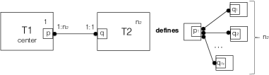
Figure 10: Star architecture style.

Example 5.

We now consider the multi-star extension of the Star architecture style, with $n$ center components of type $T_{1}$, each connected to $d$ components of type $T_{2}$ by binary connectors. As in Ex. 4, there are no other connectors. The diagram of Fig. 11 graphically describes this architecture style.

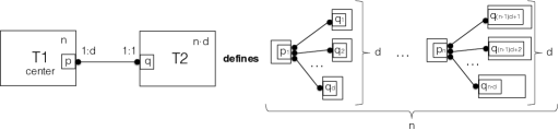
Figure 11: Multi-star architecture style.

3 Interval Architecture Diagrams

To enhance the expressiveness of diagrams we introduce interval architecture diagrams where the cardinalities, multiplicities and degrees can be intervals. With simple architecture diagrams we cannot express properties such as “component instances of type $T$ are optional”. Let us consider the example of Fig. 1 that shows four Master/Slave architectures involving two masters and two slaves. In this example, one of the masters might be optional, i.e. it might not interact with any slaves. In the first two architectures of Fig. 1 each master interacts with one slave, however, in the last two architectures one master interacts with both slaves while the other master does interacts with no slaves. In other words, the degree of $m$ varies from $0$ to $2$ and cannot be represented by an integer.

3.1 Syntax and Semantics

An interval architecture diagram $\langle\mathcal{T},n,\mathcal{C}\rangle$ consists of: 1) a set of component types $\mathcal{T}=\{T_{1},\dots,T_{k}\}$; 2) a cardinality function $n:\mathcal{T}\rightarrow\mathbb{N}^{2}$, associating, to each $T_{i}\in\mathcal{T}$, an interval $n(T_{i})=[n_{i}^{l},n_{i}^{u}]\subseteq\mathbb{N}$ (thus, $n_{i}^{l}\leq n_{i}^{u}$); 3) a set of connector motifs $\mathcal{C}=\{\Gamma_{1},\dots,\Gamma_{l}\}$ of the form $\Gamma=\Big{(}a,\{ty[m_{p}^{l},m_{p}^{u}]:ty[d_{p}^{l},d_{p}^{u}]\}_{p\in a}\Big{)}\,,$ where $\emptyset\neq a\subseteq\bigcup_{i=1}^{k}T_{i}.P$ is a generic connector and $ty[m_{p}^{l},m_{p}^{u}],ty[d_{p}^{l},d_{p}^{u}]$, with $[m_{p}^{l},m_{p}^{u}],[d_{p}^{l},d_{p}^{u}]\subseteq\mathbb{N}$ non-empty intervals and $ty\in\{mc,sc\}$ ($mc$ means “multiple choice”, whereas $sc$ means “single choice”), are, respectively, multiplicity and degree constraints associated to $p\in a$,

Semantics 2.

An architecture $\langle\mathcal{B},\gamma\rangle$ conforms to an interval architecture diagram $\langle\mathcal{T},n,\mathcal{C}\rangle$ if, for each $i\in[1,k]$, the number of components of type $T_{i}$ in $\mathcal{B}$ lies in $[n_{i}^{l},n_{i}^{u}]$ and $\gamma$ can be partitioned into disjoint sets $\gamma_{1},\dots,\gamma_{l}$, such that for each connector motif $\Gamma_{j}=\bigl{(}a,\{ty[m_{p}^{l},m_{p}^{u}]:ty[d_{p}^{l},d_{p}^{u}]\}_{p\in a}\bigr{)}\in\mathcal{C}$ and each $p\in a$: 1) there are $m_{p}\in[m_{p}^{l},m_{p}^{u}]$ instances of $p$ in each connector in $\gamma_{j}$; in case of a single choice interval the number of instances of $p$ is equal in all connectors in $\gamma_{j}$; 2) each instance of $p$ is involved in $d_{p}\in[d_{p}^{l},d_{p}^{u}]$ connectors in $\gamma_{j}$; in case of a single choice interval, the number of connectors involving an instance of $p$ is the same for all instances of $p$.

In other words, each generic port $p$ has an associated pair of intervals defining its multiplicity and degree. The interval attributes specify whether these constraints are uniformly applied or not. We write $sc[x,y]$ (single choice) to mean that the same multiplicity or degree is applied to each port instance of $p$. We write $mc[x,y]$ (multiple choice) to mean that different multiplicities or degrees can be applied to different port instances of $p$, provided they lie in the interval.

We assume that, for any two connector motifs $\Gamma_{i}=(a,\allowbreak\{ty[m_{p}^{l},m_{p}^{u}]_{i}:ty[d_{p}^{l},d_{p}^{u}]_{i}\}_{p\in a})\,\text{ for }i\in\{1,2\},$ with the same set of generic ports $a$, there exists $p\in a$ such that $[m_{p}^{l},m_{p}^{u}]_{1}\cap[m_{p}^{l},m_{p}^{u}]_{2}=\emptyset$. Similarly to simple architecture diagrams, without significant impact on the expressiveness of the formalism, this assumption greatly simplifies semantics and analysis.

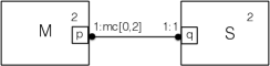
Figure 12: Architecture diagram for architectures in Fig. 1.

Example 6.

The diagram in Fig. 12 defines the set of architectures shown in Fig. 1. Notice that the degree of generic port $p$ is the multiple choice interval $[0,2]$, since one master component may be connected to two slaves, while the other master may have no connections. For the sake of simplicity, we represent intervals $[x,x]$, $mc[x,x]$ and $sc[x,x]$ as $x$.

Proposition 3.1.

Interval architecture diagrams are strictly more expressive than simple architecture diagrams.

3.2 Consistency Conditions

Similarly to simple diagrams, there are interval diagrams that do not define any architectures. Prop. 3.2 provides the necessary and sufficient conditions for the consistency of interval diagrams. A connector cannot contain more port instances than there exist in the system. Thus, the lower bound of multiplicity should not exceed the maximal number of instances of the associated component type. For all generic ports of a connector motif, there should exist a common matching factor that does not exceed the maximum number of different connectors between these ports. These conditions are a generalisation of Prop. 2.2.

To simplify the presentation we use the following notion of choice function. Let $\mathcal{I}_{T}$ and $\mathcal{I}$ be the sets of, respectively, typed intervals and intervals, as in the definition of interval diagrams above. A function $g:\mathcal{I}_{T}\rightarrow\mathcal{I}$ is a choice function if it satisfies the following constraints:

$$g(ty[x,y])=\begin{cases}[x,y],&\text{if $ty=mc$,}\\ [z,z],&\text{for some $z\in[x,y]$, if $ty=sc$.}\end{cases}$$

Proposition 3.2.

An interval architecture diagram $\langle\mathcal{T},\allowbreak n,\allowbreak\mathcal{C}\rangle$ is consistent iff, for each $T\in\mathcal{T}$, there exists a cardinality $n_{i}\in[n_{i}^{l},n_{i}^{u}]$ and, for each connector motif $(a,\{M_{p}:D_{p}\}_{p\in a})\in\mathcal{C}$ and each $p\in a$, there exist choice functions $g_{p}^{m},g_{p}^{d}$, such that, for $[m_{p}^{l},m_{p}^{u}]=g_{p}^{m}(M_{p})$ and $[d_{p}^{l},d_{p}^{u}]=g_{p}^{d}(D_{p})$ hold:

1. $m_{p}^{l}\leq n_{p}$, for all $p\in a$, (where $n_{p}=n_{i}$ for $p\in T_{i}.P$),

2. $U\cap\bigcap_{p\in a}s_{p}\neq\emptyset$, where $U=\bigl{[}1,\prod_{p\in a}\sum_{m=m_{p}^{l}}^{m_{p}^{u}}\binom{n_{p}}{m}\bigr{]}$, $\text{and}\\ s_{p}=\begin{cases}\left[\frac{n_{p}\cdot d_{p}^{l}}{m_{p}^{u}},\frac{n_{p}\cdot d_{p}^{u}}{m_{p}^{l}}\right]\cap\mathbb{N}\,,&\text{ if }m_{p}^{l}>0,\\[8.0pt] \left[\frac{n_{p}\cdot d_{p}^{l}}{m_{p}^{u}},\infty\right)\cap\mathbb{N}\,,&\text{ if }m_{p}^{l}=0.\end{cases}$

3.3 Synthesis of Configurations

The equational characterisation in Sect. 2.3 can be generalised, using systems of inequalities with some additional variables, to interval architecture diagrams. Below, we show how to characterise the configurations induced by $n$ instances of a generic port $p$ with the associated degree interval $ty[d_{p}^{l},d_{p}^{u}]$.

For a given multiplicity $m$, let $X=[x_{1},\dots,x_{w}]^{T}$ be the column vector of integer variables, corresponding to the set $\{a_{i}\}_{i\in[1,w]}$ (with $w=\binom{n_{p}}{m_{p}}$) of connectors of multiplicity $m$, involving port instances $p_{1},\dots,p_{n}$. Let $G$ be the incidence matrix $G=[g_{i,j}]_{n\times w}$ with $g_{i,j}=1$ if $p_{i}\in a_{j}$ and $g_{i,j}=0$ otherwise. The configurations induced by the $n$ instances of $p$ are characterised by the equation $GX=D$, where $D=[d_{1},\dots,d_{n}]^{T}$ and the additional (in)equalities:

$$d_{1}=\dots=d_{n}=d\text{ and }d_{p}^{l}\leq d\leq d_{p}^{u}, \text{for }ty=sc,$$ (4)

$$d_{p}^{l}\leq d_{1}\leq d_{p}^{u},\dots,d_{p}^{l}\leq d_{n}\leq d_{p}^{u}, \text{for }ty=mc.$$

Example 7.

As in Ex. 1, consider a generic port $p$ and $n_{p}=4$, $m_{p}=2$. For the degree interval $sc[1,3]$, the corresponding constraints are $1\leq d\leq 3$, $x_{1}+x_{2}+x_{3}=d$, $x_{4}=x_{3}$, $x_{5}=x_{2}$, $x_{6}=x_{1}$. For the degree interval $mc[1,3]$ the corresponding constraints are $1\leq d_{i}\leq 3$, for $i\in[1,4]$, $x_{1}+x_{2}+x_{3}=d_{1}$, $x_{1}+x_{4}+x_{5}=d_{2}$, $x_{2}+x_{4}+x_{6}=d_{3}$, $x_{3}+x_{5}+x_{6}=d_{4}$.

Suppose that the multiplicity of $p$ in the motif is given by an interval $ty[m_{p}^{l},m_{p}^{u}]$. Contrary to the degree, multiplicity does not appear explicitly as a variable in the constraints. Instead, it influences the number and nature of elements in both the matrix $G$ and vector $X$. Therefore, for single choice (i.e. $ty=sc$), the configurations induced by $n$ instances of $p$ are characterised by the disjunction of the instantiations of the system of equalities combining $G_{m}X_{m}=D$ with (4), for $m\in[m_{p}^{l},m_{p}^{u}]$. For multiple choice (i.e. $ty=mc$), all the configurations are characterised by the system combining (4) with $\sum_{m\in[m_{p}^{l},m_{p}^{u}]}(G_{m}X_{m})=D\,.$

Notice that the above modifications for interval-defined multiplicity are orthogonal to those in (4), accommodating for interval-defined degree. Similarly to the single-choice case for multiplicity, for interval-defined cardinality, the configurations are characterised by taking the disjunction of the characterisations for all values $n\in[n^{l},n^{u}]$. Based on the above characterisation for the configurations of one generic port, global configurations can be characterised by systems of linear constraints in the same manner as for simple architecture diagrams.

3.4 Architecture Style Specification Examples

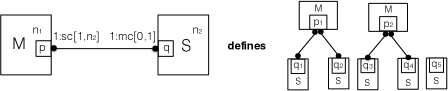
Figure 13: Master/Slave architecture style and conforming architecture.

Example 8.

The diagram of Fig. 13 describes a particular Master/Slave architecture style and a conforming architecture for $n_{1}=2$ and $n_{2}=5$.

We require that each slave interact with at most one master and that each master be connected to the same number of slaves. Multiplicities of both generic ports $p$ and $q$ are equal to $1$, allowing only binary connectors between a master and a slave. The single choice degree of generic port $p$ ensures that all port instances are connected to the same number of connectors which is a number in $[1,n_{2}]$. The multiple choice degree of generic port $q$ ensures that all port instances are connected to at most one master.

Example 9.

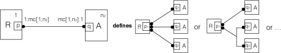
Figure 14: Repository architecture style and conforming architectures.

The diagram in the left of Fig. 14 describes the Repository architecture style involving a single instance of a component of type R and an arbitrary number $n_{2}$ of data-accessor components of type $A$. We require that all connectors involve the $R$ component. In the right of Fig. 14, we show conforming architectures for $n_{2}=3$.

Example 10.

The Map-Reduce architecture style [mapreduce] allows processing large data-sets, such as those found in search engines and social networking sites. Fig. 16 graphically describes the Map-Reduce architecture style. A conforming architecture for $n_{1}=3$ and $n_{2}=2$ is shown in Fig. 16.

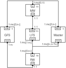
Figure 15: Map Reduce architecture style.

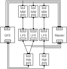
Figure 16: Map Reduce architecture.

A large dataset is split into smaller datasets and stored in the global filesystem ($GFS$). The $Master$ is responsible for coordinating and distributing the smaller datasets from the $GFS$ to each of the map workers ($MW$). The port $in$ of each $MW$ is connected to the $Mcontrol$ and $read$ ports of the $Master$ and the $GFS$, respectively. Each $MW$ processes the datasets and writes the result to its dedicated local filesystem ($LFS$) through a binary connector between their $out$ and $write$ ports. The connector is binary since no $MW$ is allowed to read the output of another $MW$. Each reduce worker ($RW$) reads the results from multiple $LFS$ as instructed by the $Master$. To this end, the $in$ port of each $RW$ is connected to the $Rcontrol$ and $read$ ports of the $Master$ and some $LFS$, respectively. Each $RW$ combines the results and writes them back to the $GFS$ through a binary connector between their $out$ and $write$ ports.

4 Checking Conformance

Algorithm 1 with polynomial-time complexity checks whether an architecture $\langle\mathcal{B},\gamma\rangle$ conforms to a simple diagram $\langle\mathcal{T},n,\mathcal{C}\rangle$. It can be easily extended for interval diagrams as shown in [MBBS16-Diagrams-TR].

Algorithm 1 checks the validity of the following three statements: 1) the number of components of each type $T$ is equal to $n(T)$; 2) there exists a partition of $\gamma$ into $\gamma_{1},\dots,\gamma_{l}$ such that each $\gamma_{i}$ corresponds to a different connector-motif $\Gamma_{i}\in\mathcal{C}$ of the diagram; 3) for each connector motif $\Gamma_{i}$ and its corresponding $\gamma_{i}$, the number of times each port instance participates in $\gamma_{i}$ satisfies the degree constraints. The three statements correspond to functions LABEL:alg:verifycardinality, LABEL:alg:verifymultiplicity and LABEL:alg:verifydegree, respectively. If all statements are valid the algorithm returns true, i.e. the architecture conforms to the diagram.

In particular, function LABEL:alg:verifycardinality takes as input the architecture diagram $\langle\mathcal{T},n,\mathcal{C}\rangle$ and the set of components $\mathcal{B}$ of the architecture $\langle\mathcal{B},\gamma\rangle$. It counts the number of components for each component type in $\mathcal{B}$ and it returns true if for each component type $\mathcal{T}$ of the diagram its cardinality matches the corresponding number of components in $\mathcal{B}$. Otherwise it returns false and algorithm 1 terminates.

Function LABEL:alg:verifymultiplicity takes as input the configuration $\gamma$ of the architecture $\langle\mathcal{B},\gamma\rangle$ and the set of connector motifs $\mathcal{C}$ of the architecture diagram $\langle\mathcal{B},\gamma\rangle$. The function checks whether there exists a partition of $\gamma$ such that each sub-configuration $\gamma_{i}$ of $\gamma$ corresponds to a distinct connector motif $\mathcal{C}_{i}$ of $\mathcal{C}$, i.e. each connector $k$ in $\gamma_{i}$ conforms to the multiplicity constraints of $\mathcal{C}_{i}$. If such a partition exists the function returns it. Otherwise, it returns $\emptyset$ and algorithm 1 terminates.

Function LABEL:alg:verifydegree takes a connector motif $\Gamma$ of $\mathcal{C}$ and its corresponding sub-configuration of $\gamma$ assigned by LABEL:alg:verifymultiplicity. For each port instance in the sub-configuration it checks whether the number of times the port participates in different connectors is equal to the corresponding degree constraint of the connector motif. If the check fails, algorithm 1 terminates.

Algorithm 1 uses a number of auxiliary functions. Function generic(p) takes a port instance and returns the corresponding generic port. Function typeof(B) returns the component type of component B. Operation map[key]++ increases the value associated with the key by one if the key is in the map, otherwise it adds a new key with value $1$.

Data: Architecture $\langle\mathcal{B},\gamma\rangle$, diagram $\langle\mathcal{T},n,\mathcal{C}\rangle$

Result: Returns $true$ if the architecture satisfies the diagram $\langle\mathcal{T},n,\mathcal{C}\rangle$. Otherwise returns $false$.

if not VerifyCardinality($\mathcal{B}$, $\langle\mathcal{T},n,\mathcal{C}\rangle$) then

          return $false$;

         

$\mathcal{S}_{\gamma}\longleftarrow$ VerifyMultiplicity($\gamma$, $\mathcal{C}$);

if $\mathcal{S}_{\gamma}=\emptyset$ then

          return $false$;

         

[1pt] for $\Gamma\in\mathcal{C}$ do

          if not VerifyDegree($\mathcal{S}_{\gamma}[\Gamma],\Gamma$) then

                   return $false$;

                  

         

return $true$;

Algorithm 1 VerifyArchitecture