New Method for Building Geodesic Lines in Riemann Geometry

New perspective form of equations for geodesic lines in Riemann Geometry was found.

Keywords: Riemann Geometry, geodesic lines, differential coordinates

1 Introduction

This work is a result of the development of the Method of Differential Coordinates (MDC) that has been designed as a method for solving differential equations [1] [2]. As we know, the majority of physical processes are described by differential equations in partial derivatives of second order linear with respect to second derivatives. The analytical stage of solving problems with equations of this type was important until recently when computers gained capacity to use these equations without preliminary analytical processing. But even nowadays, direct numerical (grid) calculation is not always possible and is not always expedient, especially because it masks the physics of the process and does not explain why the result of the calculation is what it is. That is why analytical methods (and MDC is partially one of them) are still very important. However, the present work is not devoted to the subject of differential equations, although its mathematical foundation is laid there. Previous tasks required the use of attributes of variational computation (geodesic lines), which is understandable, even familiar, in a sense. However, the specifics of MDC allow for a new outlook at what seems to be well-established stereotypes.

In the process of using MDC, the computer simultaneously builds couples of geodesic lines that are connected to each other by the very process of their building. The method of their building does not use any equations that used to be employed for computation of separate geodesic lines. The transition from conjugate calculations of several close geodesic lines to calculation of one solitary line is, in fact, the task of the present work. It is achieved by extreme convergence, integration of a couple of geodesic lines. Let us note that the possibility of determining extremals’ trajectories by combined analysis of course of their pairs has been shown by Christiaan Huygens explanation of light wave flow forms long before creation of Riemannian geometry [3].

But the main idea of this work – the one that is also the basis for MDC – is connected with the introduction and application of differential coordinates.

2 Differential Coordinates and their Properties

The fundamentals of MDC are described in a number of the author’s works, [1] in particular. Here are just the summaries, to avoid repetitions and complication of the text.

MDC grounds in the fact that a derivative, as a concept, needs only availability of the argument’s differential but not necessarily its existence as a non-zero value. Therefore, if in a coordinate space $x$ (that is $x_{1},x_{2},\dots x_{n}$) is given a differential field $dy$ (that is $dy_{1},dy_{2},\dots dy_{n}$), where

$$dy_{i}=\sum\alpha_{ij}(x)dx_{j},$$ (1)

then a derivative of any function $f(x)$ for any $dy_{i}$ can be determined as

$$\frac{Df(x)}{Dy_{i}}=\lim_{x^{\prime}\to x}\frac{f(x)-f(x^{\prime})}{\int_{x^{\prime}}^{x}dy_{i}}$$ (2)

without requirement that differentials $dy_{i}$ are complete, i.e. without requirement of existence of values $y_{i}$ (the only important condition is equality of all $dy_{j}=0$ at $j\neq i$ on the path of integration from $x^{\prime}$ to $x$ along coordinates’ line of coordinate $dy_{i}$). Taking this factor into account expands the concept of the derivative, and, at that, operator $\frac{\partial}{\partial x_{j}}$ becomes a special case of the operator $\frac{D}{Dy_{j}}$. Summation in (1) and below is conducted by repeating indexes from 1 to $n$.

Squaring the elementary distance in coordinates $dy_{i}$, that is $\sum dy_{k}^{2}=ds^{2}$, after applying here (1) will look like:

$$ds^{2}=\sum\rho_{ij}(x)dx_{i}dx_{j},$$ (3)

where $\rho_{ij}=\sum\alpha{k_{i}}\alpha{k_{j}}$. It is evident that this way the original formula of Riemann geometry is created. If (3) is given initially, then $dy_{i}$ through $\rho_{ij}$ is found by applying in (3) the expression of the reverse transition - from $dx_{j}$ to $dy_{i}$.

$$dx_{i}=\sum\alpha_{ik}^{*}dy_{k},$$ (4)

and then $\alpha_{ik}^{*}$ follow from the system of equations $\sum\rho_{ij}\alpha_{ik}^{*}\alpha_{j\nu}^{*}=\delta_{k\nu}$.

Coordinates $dy_{i}$ can be converted to $dy_{j}^{\prime}$ (which is isometric to $dy_{i}$) by conventional way of rotation: $dy_{i}^{\prime}=\sum\beta_{ij}dy_{j}$, then from condition $\sum dy_{i}^{2}=\sum dy_{j}^{\prime 2}$ follows $\sum\beta_{ij}\beta_{ik}=\delta_{jk}$. It is easy to see that operator $\Delta y$ is covariant in such transformations, it retains its form.

It is shown in [1] that in every point $x$ for every function that has any non-zero first derivatives in this point, is possible to define the gradient on the basis of $dy_{j}^{\prime}$ as the only coordinate $dy_{j}^{\prime}$ along which this function has a non-zero derivative. Note that in the case of complex functions the additional condition is that the function is analytic.

Also, we can show from (2) that the gradient’s square, that is $\sum(\frac{Df}{Dy_{i}})^{2}$, is an invariant for rotation transformations, along with $ds^{2}$.

The important property of the differential coordinates is that if in every point of solution they are rotated in such a way so one of them would be directed along function’s gradient, then the differential equation in partial derivatives for this function, written via given coordinates, becomes an equation similar to an ordinary (one-dimensional) differential equation.

3 Geodesic Lines and their Properties

If every element of the path in a given space is correlated with length $ds$, then lengths of all possible curves (including extreme, geodesic curves) are implicitly defined. In papers [1] [2], analysis of such curves was conducted for solving differential equations. Here we have a different task, but both topics are equally dealing with geodesic curves’ properties.

Let’s assume that in $n$-dimensional space with specified parameters of the medium, i.e. with a specifically defined equation (3), from point $x_{0}$ comes a system of geodesic lines, and thus $x$ is given a function in every point
$S(x_{0},x)=\int_{x_{0}}^{x}ds$ , where integration is from point $x_{0}$ - the source of geodesic lines – to the given point $x$ along the corresponding geodesic curve. Then closed $(n-1)$-dimensional hypersurfaces surrounding point $x_{0}$ where $S$=const will also be defined. Additionally, the system of coordinates $dy_{i}^{\prime}$ will be partially defined. If, for example, $dy_{1}^{\prime}$ is oriented along gradient of function $S(x)$, then all other $dy_{i}^{\prime}$ will fall into the area $S=const$.

Let us note two properties that occur in the system of geodesic lines in question, considering, for example, a two-dimensional case, when hypersurfaces $S=const$ are one-dimensional curves (Fig.1).

Increase of value $S$ (which is dictated by integration of any two fixed hypersurfaces $S=const$) will be the same along all geodesic lines. After all, this increase, i.e. the difference of integrals $\int_{x_{0}}^{x}ds$, for example between lines $S_{3}=const$ and $S_{4}=const$, will be $S_{4}-S_{3}$, no matter which geodesic line we take. That is why given differences of integrals on segments between two fixed hypersurfaces $S=const$ are the same for all geodesic lines.

Furthermore, the gradient of value $S(x)$ in “$y$-metrics” will be always directed along geodesic line. Indeed, the neighborhood area of current point $x$ without its one-dimensional subspace – vector $dS$, where $S=const$, – has $(n-1)$ dimensions. And the neighborhood area, that has dimension along direction of gradient $S$ extracted and is left with only part of space where $S=const$, is also $(n-1)$-dimensional; i.e. these two $(n-1)$-dimensional subspaces coincide. Therefore, two one-dimensional subspaces – vector $dS$ and gradient $S$ – have to coincide too, which means coincidence of directions of gradient $S(x)$ and the geodesic line.

Fig. 1 shows how geodesic lines curve in the area between $S_{1}$ and $S_{2}$ assuming that functions $S(x_{0},x)$ and $\alpha(x)$ are either real or are projections of real parts of complex $S$, $\alpha$ onto space of real values $x_{i}$. There two close to each other geodesic lines cross also close to each other hypersurfaces $S_{1}$ and $S_{2}$. Let’s define the geodesic lengths that are count off point $x_{0}$ in “$x$-metrics” as $r_{1}x$, $r_{2}x$, and the angle between axis $x_{2}$ and $dr_{i}$ as $F_{i}$. If we turn coordinates $x$ in some point of the geodesic line in such a way that the new differential $dx_{1}^{\prime}$ is directed along this line, then we get a corresponding factor $\alpha(x)$ for equation that connects the element $dy_{1}^{\prime}=dS$ along the geodesic line with $(dx_{1}^{\prime})_{i}=dr_{i}$ , and equation (1) for $dy_{1}^{\prime}$ will become $dS=\alpha(x)dr_{i}$. Increase of value $S$ between $S_{1}$=const and $S_{2}=$const for both curves is $\delta S=S_{2}-S_{1}$, i.e. values $\delta S=\alpha(x^{\prime})\delta r_{1}$ and $\delta S=\alpha(x^{\prime\prime})\delta r_{2}$ for both of them are the same; but as $\alpha(x^{\prime})$ and $\alpha(x^{\prime\prime})$ are different, the values $\delta r_{1}$ and $\delta r_{2}$ are different too.

Without knowing how the angle $F$ of vector $dr$ of every geodesic will change between $S_{1}$ and $S_{2}$, we can draw zones’ borders on their ends in $S_{1}$ that will correspond with given value $\delta S$.

For simplicity, on Fig.1 these borders are shown as circles, although it is possible for them to take shape of deformed circles (like ellipses) if $\alpha$ will depend also on direction of vector $dr$. But that has no basic importance. The curve $S_{2}$ (i.e. hypersurface $S_{2}$) can only touch these zones’ borders or there would be shorter ways to $S_{2}$ than geodesic lines, and that is impossible. Based on that, we can calculate $\delta F$ – variation of angular orientation of elements $dr_{i}$ in the ends of given couple of geodesics [1] after passing the distance from $S_{1}$ to $S_{2}$.

Small quantity $\delta F$ is generated by two small quantities:
$\lambda=[(x_{2}^{\prime\prime}-x_{2}^{\prime})^{2}+(x_{1}^{\prime\prime}-x_{1}^{\prime})^{2}]^{\frac{1}{2}}$ (the result of initial divergence of geodesic lines in point $x_{0}$) and $\delta r_{1}$ (the result of divergence of $S_{2}$ from $S_{1}$). Up to second order values, small quantity $\delta F$ is connected to $\lambda$ and $\delta r_{1}$ with equation [1] [2]

$$\sin(\delta F)=\frac{\delta r_{1}\{\frac{\alpha(x^{\prime})}{\alpha(x^{\prime\prime})}-1\}}{\lambda}.$$

Expanding $sin(\delta F)$ in a row and tending $\lambda$ and $\delta r_{1}$ by turns to zero, we have:

$$\frac{dF}{dr}=\frac{\alpha^{\prime}}{\alpha},$$ (5)

where $\alpha^{\prime}$ is a derivative of $\alpha$ with respect to orthogonal to $\delta r_{1}$ in “$x$-metrics” in direction of gradient $\alpha$ (the result of the operation $\lambda\to 0$). From here, knowing that $\frac{dx_{2}}{dr}=\cos F$ , differentiating it one more time in $r$, and taking in account (5), we find:

$$\frac{d^{2}x_{2}}{dr^{2}}=-\frac{\alpha^{\prime}}{\alpha}\sqrt{1-\Big{(}\frac{dx_{2}}{dr}\Big{)}^{2}}.$$ (6)

Naturally, the analog of this formula may be written also for $\frac{d^{2}x_{1}}{dr^{2}}$. In principle, the root in the right part of (6) can be substituted for $\frac{dx_{1}}{dr}$, and then (6) will become linear with respect to derivative of $x_{1}$. But the value of the variant (6) lies in dealing only with derivatives in one coordinate, the very coordinate that interests us at this moment.

When $n>2$, a two-dimensional space should be allocated with respect to vectors $dr$ and $dx_{j}$ in the neighborhood of the geodesic line. Then temporarily introducing second (intermediary) coordinate of type $x_{t}$ , we can obtain an equation (6) for $x_{j}$. As a result, the geodesic will be defined by $n$ equations

$$\frac{d^{2}x_{j}}{dr^{2}}=-\frac{\alpha^{\prime}}{\alpha}\sqrt{1-\Big{(}\frac{dx_{j}}{dr}\Big{)}^{2}},$$ (7)

where the derivative from $\alpha$ is always taken in a crosswise direction to $dr$ in an element of a two-dimensional surface that was created by vectors $dr$ and $dx_{j}$. Conceptually, the gradient $\alpha$ curves the geodesic in the plane of the gradient’s “pressure” on it.

Formula (7) has a very clear meaning. The square root is the cosine of an angle between the gradient of function $\alpha(x)$ and vector $dr$ normal. It is evident that gradient’s component along $dr$ does not change its alignment, and orthogonal to $dr$ component pulls this vector to itself.

Value $\alpha(x)$ that appears in (6) and (7) is introduced by connecting $dy_{1}^{\prime}$ and $dr$ with the equation $dy_{1}^{\prime}=\alpha(x)dr$. But $ds^{2}=(dy_{1}^{\prime})^{2}=\alpha^{2}dr^{2}$ . That is why if we are given a particular orientation of vector $dr$ (and particular values $\frac{dx_{j}}{dr}$ along with it) and also space metrics are predetermined by formula (3), then by placing $dx_{k}=\frac{dx_{k}}{dr}dr$ in it and taking into account the equation $ds^{2}=\alpha^{2}dr^{2}$, we have

$$\alpha=\sqrt{\sum\rho_{ij}(x)(\frac{dx_{i}}{dr})(\frac{dx_{j}}{dr})}.$$

Clearly, the absence of additional cumbersome calculations makes (7) very convenient to use. Now, let’s remember that Fig. 1 was built for real terms $S$ and $\alpha$. But if equation (6) and function $S(x)$ are analytical, than generalization (7) for complex $\alpha$, $x_{i}$ have to fully satisfy conditions of extremum (minimum) when its real term satisfies these conditions. At that, functions and their derivations maintain their values, and that secures the equations formed from them. As is well known, Riemannian geometry analogue of (7) which is grounded in customary conceptions of parallel transport of a vector along geodesic line, looks like

$$\frac{d^{2}x_{i}}{ds^{2}}+\sum\Gamma_{\alpha\beta}^{i}(\frac{dx_{\alpha}}{ds})(\frac{dx_{\beta}}{ds})=0,$$ (8)

where $\Gamma_{\alpha\beta}^{i}$ is the Cristoffel symbol which is denoted in cumbersome manner by $\rho_{ij}$ and their derivatives with respect to $x_{v}$ . Nowadays, (8) has become one of the pillars for the theory of vector and tensor analysis. The conclusion (7), drawn from a different principle, is simpler, and the formula itself is more understandable.

What comes to mind when we compare these formulas? They are interchangeable, but (7) might have an advantage over (8), as it can be more convenient to use. In particular, it can be used to illustrate and explain results of application of (8). Let’s note that (7) and (8) were tested during deduction of Snell’s law, which is well known in radio-physics. Both of them have proved the law to be true. (7) has proved the law immediately, and (8) after long laborious computations. It is evident that (7) is highly promising for theoretical and practical physics. Moreover, because of its clarity, it is very convenient for fast qualitative valuations prior to final precise calculations.

Let’s emphasize the following: (8) had served as a basis for the creation of general theory of relativity; perhaps (7) will prove to be helpful for development in this direction.

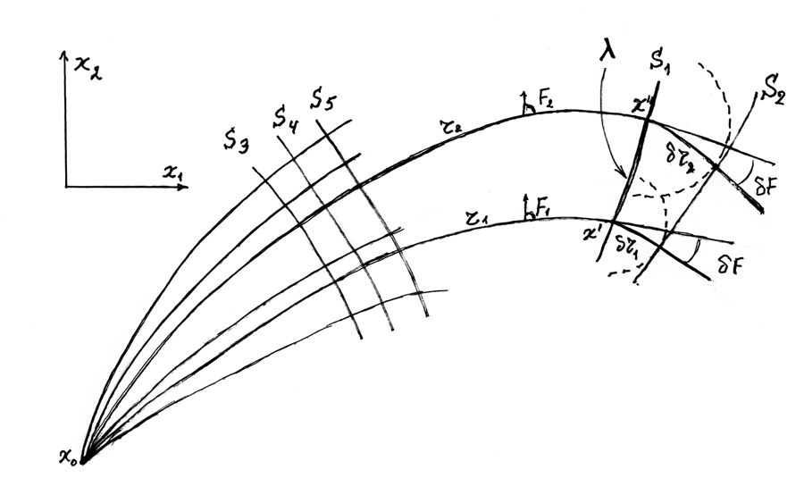
Figure 1:

References

- [1] Victor I. Pogorelov, Solving Problems of Mathematical Physics by the Method of Differential Coordinates. Moscow, Sputnik+, 2007. .
- [2] Victor I. Pogorelov, The Method of Differential Coordinates and It’s Application for Solving Problems of Mathematical Physics. Moscow, Sputnik+, 2008
- [3] Christiaan Huygens, Traité de la lumière… Haag, 1690.