Combination of LMS Adaptive Filters
with Coefficients Feedback

Luiz F. O. Chamon,  and Cássio G. Lopes Signal Processing Lab of the Department of Electronic Systems Engineering, University of São Paulo, Brazil. e-mail: chamon@usp.br and cassio@lps.usp.br. Part of the results in this paper appeared in [19].
Abstract

Parallel combinations of adaptive filters have been effectively used to improve the performance of adaptive algorithms and address well-known trade-offs, such as convergence rate vs. steady-state error. Nevertheless, typical combinations suffer from a convergence stagnation issue due to the fact that the component filters run independently. Solutions to this issue usually involve conditional transfers of coefficients between filters, which although effective, are hard to generalize to combinations with more filters or when there is no clearly faster adaptive filter. In this work, a more natural solution is proposed by cyclically feeding back the combined coefficient vector to all component filters. Besides coping with convergence stagnation, this new topology improves tracking and supervisor stability, and bridges an important conceptual gap between combinations of adaptive filters and variable step size schemes. We analyze the steady-state, tracking, and transient performance of this topology for LMS component filters and supervisors with generic activation functions. Numerical examples are used to illustrate how coefficients feedback can improve the performance of parallel combinations at a small computational overhead.

Index Terms:
Adaptive filters, combination of adaptive filters, coefficients feedback, affine combination, convex combination.

I Introduction

Adaptive filters (AFs) are widely used in signal processing due to their tracking capabilities and low computational complexity. Still, they display performance trade-offs that can hinder their use in practice, such as the compromise between convergence rate or tracking and steady-state error [1, 2]. These issues have been mitigated by modifying the filter cost functions, e.g., mixed-norm AFs, or by using variable step size (VSS) techniques [3, 4, 5, 6, 7]. More recently, combinations of AFs were introduced to address these trade-offs, especially in situation where the design of a single filter is intricate [8, 9, 10, 11, 12, 13, 14, 15, 16, 17, 18, 19, 20, 21, 22]. In this approach, a pool of AFs is combined by an adaptive supervisor such that the overall system performs at least as well as the best filter in the pool, usually in the mean-square error (MSE) sense. Typically, convex or affine supervisors are used, possibly in their normalized forms [10, 12, 23, 24].

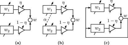
The most common combination structure runs each AF independently and then merges their outputs (Fig. 1a). We dub this structure parallel-independent. It has been studied for different adaptive algorithms, step sizes, orders, and supervisors [8, 9, 10, 11, 16, 14, 12, 13, 15]. Although effective, parallel-independent combinations display a well-known convergence stagnation regardless of the supervisor. To understand this phenomenon, consider a combination of two AFs, one fast and one slow but accurate (Fig. 3a). Once the faster AF has converged, the output of the combination plateaus while the slower filter does not reach a lower error level. When this happens, the combination “switches” filters and continues to converge.

Structural changes have been proposed to address this issue. In [10], conditional coefficients leakage from faster to more accurate AF was introduced (Fig. 1b). This approach modifies the recursion of the slower AF so that its coefficient vector becomes a mixture of those from both component filters. A similar idea was explored in [21] where the coefficients of the slower filter were conditionally replaced by those from the faster one. A different approach entirely reformulated the topology leading to incremental combinations [18, 20].

A more natural solution that retains the parallel form of the combination was put forward in [19]: cyclic coefficients feedback (Fig. 1c). This structure periodically feeds back the overall coefficients of the combination to all component filters, improving their performance regardless of which AF is better at each iteration. The cyclic nature of these feedbacks is the key to exploit the output of the combination without hindering the supervisor adaptation. This topology not only addresses the convergence stagnation issue, but also improves tracking performance. In this work, we analyze this structure by

  • showing that VSS adaptive algorithms can be interpreted as combinations with coefficients feedback;

  • analyzing the steady-state, tracking, and transient performance of parallel combinations of LMS filters with coefficients feedback;

  • extending the supervisor transient model from [25] to general activation functions;

  • using these analyses to show that besides eliminating the stagnation issue, coefficients feedbacks increase cooperation among filters, improve tracking, and stabilize the supervising parameters;

  • illustrating the performance of this new topology in numerical examples.

Notation: Lowercase boldface letters represent vectors (𝒙𝒙\bm{x}) and uppercase boldface letters are used for matrices (𝑿𝑿\bm{X}). Iteration indices are shown as subscripts on vectors (𝒙isubscript𝒙𝑖\bm{x}_{i}) and in parenthesis for scalars [x(i)𝑥𝑖x(i)]. We denote the steady-state value of any variable by omitting its iteration index, i.e., x=limix(i)𝑥subscript𝑖𝑥𝑖x=\lim_{i\to\infty}x(i).

Refer to caption
Figure 1: Parallel topologies: (a) Parallel-independent; (b) Parallel with transfers of coefficients—leakage or handover; (c) Parallel with coefficients feedback.

II Combinations of Adaptive Filters

A combination of AFs is composed of three parts: the component filters, the topology, and the supervisor. Component filters are the building blocks of combinations: they are the standalone AFs that are merged to improve their individual performances. The manner in which these AFs are merged is called the topology. It defines how the filters interact and how the output of the combination is obtained from the output of each AF. Oftentimes this topology depends on a set of parameters that modifies the combination behavior. These supervising parameters are adapted by the supervisor. In the sequel, we examine each of these elements individually, starting with the component filters.

II-A The component filters

In a combination of N𝑁N AFs, each component filter is distinguished by using the index n=1,,N𝑛1𝑁n=1,\dots,N. These AFs update a priori coefficient vectors 𝒘n,aMsubscript𝒘𝑛𝑎superscript𝑀\bm{w}_{n,a}\in\mathbb{R}^{M} in an attempt to minimize some underlying cost function Jn(𝒘n,a)subscript𝐽𝑛subscript𝒘𝑛𝑎J_{n}(\bm{w}_{n,a}). This cost function is usually the MSE Jn(𝒘n,a)=𝔼[d(i)𝒖iT𝒘n,a]2J_{n}(\bm{w}_{n,a})=\operatorname{\mathbb{E}}\left[d(i)-\bm{u}_{i}^{T}\bm{w}_{n,a}\right]^{2}, where 𝒖isubscript𝒖𝑖\bm{u}_{i} is a M×1𝑀1M\times 1 real-valued regressor vector and d(i)𝑑𝑖d(i)\in\mathbb{R} is the desired signal. For example, in a combination of LMS filters, the recursion of the n𝑛n-th AF is written as

𝒘n,i=𝒘n,a+μn𝒖i[d(i)𝒖iT𝒘n,a],subscript𝒘𝑛𝑖subscript𝒘𝑛𝑎subscript𝜇𝑛subscript𝒖𝑖delimited-[]𝑑𝑖superscriptsubscript𝒖𝑖𝑇subscript𝒘𝑛𝑎,\bm{w}_{n,i}=\bm{w}_{n,a}+\mu_{n}\bm{u}_{i}\left[d(i)-\bm{u}_{i}^{T}\bm{w}_{n,a}\right]\text{,} (1)

where μn>0subscript𝜇𝑛0\mu_{n}>0 is a step size. Using the a priori coefficients 𝒘n,asubscript𝒘𝑛𝑎\bm{w}_{n,a} in (1) we can formalize the notion of combination topology.
Refer to caption
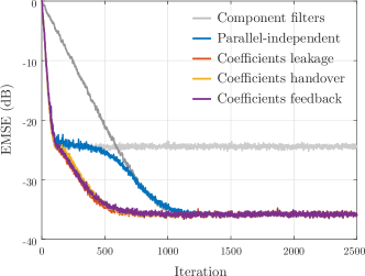
Figure 2: Effect of different topologies on the supervisor performance (convex supervisor). White stationary scenario: M=10𝑀10M=10, σu2=1superscriptsubscript𝜎𝑢21\sigma_{u}^{2}=1, σv2=102superscriptsubscript𝜎𝑣2superscript102\sigma_{v}^{2}=10^{-2}, μ1=0.05subscript𝜇10.05\mu_{1}=0.05, μ2=0.005subscript𝜇20.005\mu_{2}=0.005; Parallel-independent: μa=200subscript𝜇𝑎200\mu_{a}=200; Coefficients leakage: μa=450subscript𝜇𝑎450\mu_{a}=450 and α=0.6𝛼0.6\alpha=0.6 for η0.98𝜂0.98\eta\geq 0.98 and α=0𝛼0\alpha=0 otherwise; Coefficients handover: L=10𝐿10L=10 and μa=200subscript𝜇𝑎200\mu_{a}=200; Cyclic coefficients feedback: L=90𝐿90L=90 and μa=270subscript𝜇𝑎270\mu_{a}=270.
Refer to caption
Figure 3: Combination of LMS filters with cyclic coefficients feedback. White stationary scenario (see Section VI): M=7𝑀7M=7, σu2=1superscriptsubscript𝜎𝑢21\sigma_{u}^{2}=1, σv2=102superscriptsubscript𝜎𝑣2superscript102\sigma_{v}^{2}=10^{-2}, μ1=0.05subscript𝜇10.05\mu_{1}=0.05, and μ2=0.005subscript𝜇20.005\mu_{2}=0.005. (a) Parallel-independent (L𝐿L\to\infty): μa=200subscript𝜇𝑎200\mu_{a}=200 (convex supervisor); (b) Cyclic coefficients feedback: L=50𝐿50L=50 and μa=200subscript𝜇𝑎200\mu_{a}=200 (convex supervisor); (c) Coefficients feedback: L=1𝐿1L=1 and μa=300subscript𝜇𝑎300\mu_{a}=300 (convex supervisor).

II-B The topology

Notice from (1) that AFs have 3 inputs: the regressor 𝒖isubscript𝒖𝑖\bm{u}_{i}, the desired signal d(i)𝑑𝑖d(i), and the a priori coefficient vector 𝒘n,asubscript𝒘𝑛𝑎\bm{w}_{n,a}. Filters in a combination interact using the latter. In fact, the topology of a combination is formally defined by specifying the 𝒘n,asubscript𝒘𝑛𝑎\bm{w}_{n,a} and a function that maps the component filters to the output of the combination. In this work, we focus on parallel topologies, i.e., those for which the update (1) can be evaluated for all n𝑛n simultaneously. Formally, a parallel topology is one in which the {𝒘n,a}subscript𝒘𝑛𝑎\{\bm{w}_{n,a}\} at iteration i𝑖i are functions only of the {𝒘n,j}subscript𝒘𝑛𝑗\{\bm{w}_{n,j}\} for j<i𝑗𝑖j<i. This is in contrast to incremental or series topologies, in which the update of a component filter may depend on the state of another AF at the current iteration [18]. We define the output of parallel combinations as

𝒘i=n=1Nηn(i)𝒘n,i,subscript𝒘𝑖superscriptsubscript𝑛1𝑁subscript𝜂𝑛𝑖subscript𝒘𝑛𝑖,\bm{w}_{i}=\sum_{n=1}^{N}\eta_{n}(i)\bm{w}_{n,i}\text{,} (2)

where 𝒘isubscript𝒘𝑖\bm{w}_{i} is the global coefficient vector and {ηn(i)}subscript𝜂𝑛𝑖\{\eta_{n}(i)\} are the supervising parameters.

The most common parallel topology is the parallel-independent, where 𝒘n,a=𝒘n,i1subscript𝒘𝑛𝑎subscript𝒘𝑛𝑖1\bm{w}_{n,a}=\bm{w}_{n,i-1} (Fig. 1a). In other words, the component filters run independently and their cooperation arises solely at the output of the combination (2[10, 12, 13, 25, 26, 27]. This structure suffers from a well-known convergence stagnation issue illustrated in Fig. 3a. Notice that the overall combination appears to stall as the faster filter approaches steady-state until the slower filter output error catches up. Although this effect is more prominent in stationary scenarios, it occurs for all common supervisors and suggests that structural changes are required to overcome it.

In [10], convergence stagnation was addressed using a conditional coefficients leakage scheme (Fig. 1b). Assuming filter 222 is slower and more accurate, this topology adapts filter 111 independently, i.e., 𝒘1,a=𝒘1,i1subscript𝒘1𝑎subscript𝒘1𝑖1\bm{w}_{1,a}=\bm{w}_{1,i-1}, and changes the second filter recursion to

𝒘2,isubscript𝒘2𝑖\displaystyle\bm{w}_{2,i} =α𝒘1,i1+(1α)[𝒘2,i1+μ2𝒖ie2(i)],absent𝛼subscript𝒘1𝑖11𝛼delimited-[]subscript𝒘2𝑖1subscript𝜇2subscript𝒖𝑖subscript𝑒2𝑖,\displaystyle=\alpha\bm{w}_{1,i-1}+(1-\alpha)[\bm{w}_{2,i-1}+\mu_{2}\bm{u}_{i}e_{2}(i)]\text{,} (3)

where e2(i)=d(i)𝒖iT𝒘2,i1subscript𝑒2𝑖𝑑𝑖superscriptsubscript𝒖𝑖𝑇subscript𝒘2𝑖1e_{2}(i)=d(i)-\bm{u}_{i}^{T}\bm{w}_{2,i-1}, α=α¯𝕀η(i)>ηth𝛼¯𝛼subscript𝕀𝜂𝑖subscript𝜂th\alpha=\bar{\alpha}\,\mathbb{I}_{\eta(i)>\eta_{\text{th}}}, for constants α¯[0,1]¯𝛼01\bar{\alpha}\in[0,1] and ηth1subscript𝜂th1\eta_{\text{th}}\approx 1, and 𝕀𝕀\mathbb{I} denotes the indicator function. It is straightforward to see why the threshold test in the indicator function is paramount: unless α𝛼\alpha vanishes, filter 111 will perturb the steady-state of filter 222 and the overall combination will eventually be worse than the second filter alone.

An alternative transfer of coefficients was proposed [21]. Coefficients handover once again assumes that the component filter 222 is slower and more accurate and cyclically and conditionally assigns 𝒘2,i=𝒘1,isubscript𝒘2𝑖subscript𝒘1𝑖\bm{w}_{2,i}=\bm{w}_{1,i}. Although it uses the same condition as in the coefficients leakage scheme, this solution is more effective in addressing the convergence stagnation issue. Moreover, it can also be seen as a complexity reduction technique since the second component is not updated when handover occurs [21].

Though effective (see Fig. 2), these methods have downsides from an application point of view. In particular, they are based on unidirectional transfers, i.e., from filter 111 to filter 222. It may however be hard to guarantee in practice that filter 111 will always be faster. This is the case, for instance, in tracking applications or varying signal-to-noise ratio (SNR). This issue is further accentuated in combinations with N>2𝑁2N>2 AFs in which there are N(N1)𝑁𝑁1N(N-1) possible transfers to choose from. Moreover, these techniques regularly require conditional tests to check whether transfers should take place, which places an additional burden on the implementation.

Before we show how a topology with coefficients feedback addresses these issues, we explain the final element of combinations, the supervisor.

II-C The supervisor

The supervisor is responsible for adjusting the supervising parameters of the topology, playing a fundamental role in the combination performance. The most common approach is to adapt ηn(i)subscript𝜂𝑛𝑖\eta_{n}(i) in (2) so as to minimize the global MSE 𝔼e(i)2𝔼𝑒superscript𝑖2\operatorname{\mathbb{E}}e(i)^{2} under an unbiasedness constraint, where e(i)=d(i)𝒖i𝒘i1𝑒𝑖𝑑𝑖subscript𝒖𝑖subscript𝒘𝑖1e(i)=d(i)-\bm{u}_{i}\bm{w}_{i-1} is the global output estimation error. For parallel topologies, this constraint can be expressed as [10, 12, 26]

n=1Nηn(i)=1,for all i.superscriptsubscript𝑛1𝑁subscript𝜂𝑛𝑖1,for all 𝑖.\sum_{n=1}^{N}\eta_{n}(i)=1\text{,}\quad\text{for all }i\text{.} (4)

Without loss of generality, the remain of this paper considers the N=2𝑁2N=2 case, given that larger combinations can be built from smaller ones using hierarchical combination techniques [14, 15]. Using (4), the global coefficient vector in (2) therefore reduces to

𝒘i=η(i)𝒘1,i+[1η(i)]𝒘2,i.subscript𝒘𝑖𝜂𝑖subscript𝒘1𝑖delimited-[]1𝜂𝑖subscript𝒘2𝑖.\bm{w}_{i}=\eta(i)\,\bm{w}_{1,i}+\left[1-\eta(i)\right]\bm{w}_{2,i}\text{.} (5)

The global MSE minimization is typically carried out using stochastic gradient descent, mirroring the adaptation of standalone AFs such as (1). Additionally, a strictly increasing activation function f𝑓f can be used to reduce the variance of the supervising parameters, in which case the supervisor adapts an internal state a𝑎a that determines η(i)𝜂𝑖\eta(i). This general supervising parameter adaptation procedure can be described as

a(i)𝑎𝑖\displaystyle a(i) =a(i1)+μae(i)[y1(i)y2(i)]f[a(i1)]absent𝑎𝑖1subscript𝜇𝑎𝑒𝑖delimited-[]subscript𝑦1𝑖subscript𝑦2𝑖superscript𝑓delimited-[]𝑎𝑖1\displaystyle=a(i-1)+\mu_{a}e(i)\left[y_{1}(i)-y_{2}(i)\right]f^{\prime}[a(i-1)] (6a)
η(i)𝜂𝑖\displaystyle\eta(i) =f[a(i)],absent𝑓delimited-[]𝑎𝑖,\displaystyle=f\left[a(i)\right]\text{,} (6b)

where yn=𝒖iT𝒘n,i1subscript𝑦𝑛superscriptsubscript𝒖𝑖𝑇subscript𝒘𝑛𝑖1y_{n}=\bm{u}_{i}^{T}\bm{w}_{n,i-1} is the output of the n𝑛n-th component, μa>0subscript𝜇𝑎0\mu_{a}>0 is a step size, and fsuperscript𝑓f^{\prime} denotes the derivative of f𝑓f [14, 16]. The auxiliary variable a𝑎a is usually restricted to some range [a,a+]superscript𝑎superscript𝑎[a^{-},a^{+}] by saturating (6a). Note that the restrictions on f𝑓f imply that f>0superscript𝑓0f^{\prime}>0 and guarantees that (6a) descends along the gradient and avoids stalling the adaptation algorithm. In other words, it ensures that there is no a𝑎a for which f(a)superscript𝑓𝑎f^{\prime}(a) vanishes and the supervising parameter becomes independent of the component filters.

For appropriate choices of the activation function in (6) we can recover the two most widely used supervising algorithms. The affine supervisor is obtained by letting f(a)=a𝑓𝑎𝑎f(a)=a in (6) and reads

η(i)=η(i1)+μηe(i)[y1(i)y2(i)].𝜂𝑖𝜂𝑖1subscript𝜇𝜂𝑒𝑖delimited-[]subscript𝑦1𝑖subscript𝑦2𝑖.\eta(i)=\eta(i-1)+\mu_{\eta}e(i)\left[y_{1}(i)-y_{2}(i)\right]\text{.} (7)

The value of η(i)𝜂𝑖\eta(i) is typically constrained to improve steady-state stability by, for instance, taking η(i)[0.2,1.2]𝜂𝑖0.21.2\eta(i)\in[-0.2,1.2] [12, 28]. The convex supervisor takes f𝑓f to be a sigmoidal function, so that (6) becomes

a(i)𝑎𝑖\displaystyle a(i) =a(i1)+μae(i)[y1(i)y2(i)]×\displaystyle=a(i-1)+\mu_{a}e(i)\left[y_{1}(i)-y_{2}(i)\right]\times
η(i1)[1η(i1)]𝜂𝑖1delimited-[]1𝜂𝑖1\displaystyle\qquad\qquad\qquad\qquad\qquad\eta(i-1)\left[1-\eta(i-1)\right] (8a)
η(i)𝜂𝑖\displaystyle\eta(i) =11+ea(i)absent11superscript𝑒𝑎𝑖\displaystyle=\dfrac{1}{1+e^{-a(i)}} (8b)

To prevent stalling, a(i)𝑎𝑖a(i) is usually restricted to [4,4]44[-4,4] either by saturating a𝑎a or modifying (8b[10, 29].

Normalized versions of supervisors (7) and (8) are obtained by taking μη,μa=μ~/p(i)subscript𝜇𝜂subscript𝜇𝑎~𝜇𝑝𝑖\mu_{\eta},\mu_{a}=\tilde{\mu}/p(i) with p(i)=βe(i)2+(1β)p(i1)𝑝𝑖𝛽𝑒superscript𝑖21𝛽𝑝𝑖1p(i)=\beta e(i)^{2}+(1-\beta)\,p(i-1) for some normalized step size μ~>0~𝜇0\tilde{\mu}>0 [23, 24, 28]. Although we use the unnormalized (6) in our analyses, we illustrate the fact that the coefficients feedback topology is effective regardless of the supervisor by also displaying results for the normalized versions.
Refer to caption
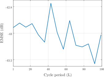
Figure 4: Steady-state performance of combinations with coefficients feedback for different L𝐿L. Correlated scenario: M=5𝑀5M=5, σu2=1superscriptsubscript𝜎𝑢21\sigma_{u}^{2}=1, σv2=102superscriptsubscript𝜎𝑣2superscript102\sigma_{v}^{2}=10^{-2}, γ=0.7𝛾0.7\gamma=0.7, μ1=0.01subscript𝜇10.01\mu_{1}=0.01, and μ2=0.002subscript𝜇20.002\mu_{2}=0.002. Convex supervisor: μa=100subscript𝜇𝑎100\mu_{a}=100. Steady-state value is an average of 1000 iterations (see Section VI).

III Cyclic Coefficients Feedback

Regardless of using convex or affine supervisors, normalized or not, convergence stagnation remains an issue in parallel-independent combinations. To mitigate this issue, a new topology was introduced in [19] as an alternative to the coefficients transfers from Section II-B. It is based on feeding back the globl coefficients to all component filters at every iteration (Fig. 1c). Formally, the a priori coefficients in (1) are defined as 𝒘n,a=𝒘i1subscript𝒘𝑛𝑎subscript𝒘𝑖1\bm{w}_{n,a}=\bm{w}_{i-1}, for 𝒘isubscript𝒘𝑖\bm{w}_{i} as in (2). This is motivated by the fact that the supervisor adapts (2) so that the global coefficients minimize the overall MSE. Hence, these feedbacks enforce that each AF in the combination updates the best available coefficient vector estimate at each iteration.

In practice, however, coefficients feedbacks have the effect of slowing down the supervisor adaptation, which degrades the combination performance (Fig. 3c). This is due to the fact that feedbacks reduces the difference between the component filters outputs yn(i)subscript𝑦𝑛𝑖y_{n}(i), since they all update the same a priori coefficients. It is then clear from (6) that the ηn(i)subscript𝜂𝑛𝑖\eta_{n}(i) will change slowly. A simple solution to this issue is to make the feedback cyclical by taking

𝒘n,a=δ(irL)𝒘i1+[1δ(irL)]𝒘n,i1,subscript𝒘𝑛𝑎𝛿𝑖𝑟𝐿subscript𝒘𝑖1delimited-[]1𝛿𝑖𝑟𝐿subscript𝒘𝑛𝑖1,\bm{w}_{n,a}=\delta(i-rL)\bm{w}_{i-1}+\left[1-\delta(i-rL)\right]\bm{w}_{n,i-1}\text{,} (9)

where L𝐿L is a constant cycle period, δ(i)𝛿𝑖\delta(i) is the Kronecker delta, and r𝑟r\in\mathbb{N} (Fig. 3b).

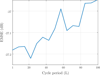
Combinations with cyclic coefficients feedback have two limiting behaviors: (i) for L=1𝐿1L=1, the relation in (9) reduces to 𝒘n,a=𝒘i1subscript𝒘𝑛𝑎subscript𝒘𝑖1\bm{w}_{n,a}=\bm{w}_{i-1} and the global coefficients are always fed back to the component filters; (ii) for L𝐿L\to\infty, we can write (9) as 𝒘n,a=𝒘n,i1subscript𝒘𝑛𝑎subscript𝒘𝑛𝑖1\bm{w}_{n,a}=\bm{w}_{n,i-1} and the usual parallel-independent combination from Section II-B is recovered. However, the advantage of coefficients feedback appear when 1<L1𝐿much-less-than1<L\ll\infty. It is worth noting that the overall performance of this topology is robust for a wide range of L𝐿L (see Figs. 4 and 5), so that values between 505050 and 150150150 typically work well. Alternatively, a procedure to design the cycle period was proposed in [19].

Coefficients feedback provides all component filters with the best coefficients estimate available to the combination, i.e., the global coefficients. Moreover, they are neither directional nor limited to any pair of component filters as in the structures from Section II-B. It is therefore straightforward to extend beyond two filter combinations. In terms of performance, this topology not only effectively addresses convergence stagnation, but can also improve the combination misadjustment, especially in nonstationary scenarios. These performance improvements are examined in the next two sections by analyzing the steady-state, tracking, and transient behavior of a combination of LMS filters with cyclic coefficients feedback. Although any AFs can be used in these combinations, we focus on LMS filters for the purpose of analysis. Before proceeding, however, we discuss a conceptual consequence of the coefficients feedback topology by formalizing the relation between combinations of AFs and VSS algorithms.
Refer to caption
Figure 5: Tracking performance of combinations with coefficients feedback for different L𝐿L. White nonstationary scenario: M=5𝑀5M=5, σu2=1superscriptsubscript𝜎𝑢21\sigma_{u}^{2}=1, σv2=102superscriptsubscript𝜎𝑣2superscript102\sigma_{v}^{2}=10^{-2}, 𝑸=105𝑰𝑸superscript105𝑰\bm{Q}=10^{-5}\bm{I}, μ1=0.07subscript𝜇10.07\mu_{1}=0.07, and μ2=0.01subscript𝜇20.01\mu_{2}=0.01. Convex supervisor: μa=100subscript𝜇𝑎100\mu_{a}=100. Steady-state value is an average of 1000 iterations (see Section VI).

III-A VSS algorithms as combinations of adaptive filters

The close relation between standalone VSS AFs and combinations of AFs was already observed in [10]. The parallel-independent topology, however, cannot be used as a step size adaptation structure. This barrier prevents, for instance, the effective use of these combinations in nonstationary scenarios. In fact, a parallel-independent combination of LMS filters can only match the tracking performance of a standalone LMS filter with an optimally designed step size μosuperscript𝜇𝑜\mu^{o} [1, Lemma 7.5.1] if one of its component filters has step size μosuperscript𝜇𝑜\mu^{o} [30].

The coefficients feedback topology bridges this conceptual and practical gap. To see how this is the case, let all AFs of a combination have update equations of the form

𝒘n,i=𝒘n,a+μn𝒑i(𝒘n,a),for n=1,,Nformulae-sequencesubscript𝒘𝑛𝑖subscript𝒘𝑛𝑎subscript𝜇𝑛subscript𝒑𝑖subscript𝒘𝑛𝑎,for 𝑛1𝑁\bm{w}_{n,i}=\bm{w}_{n,a}+\mu_{n}\bm{p}_{i}(\bm{w}_{n,a})\text{,}\quad\text{for }n=1,\dots,N

where 𝒑isubscript𝒑𝑖\bm{p}_{i} denotes the update direction at iteration i𝑖i. For example, the LMS filter in (1) is recovered by taking 𝒑i(𝒘n,a)=𝒖i[d(i)𝒖iT𝒘n,a]subscript𝒑𝑖subscript𝒘𝑛𝑎subscript𝒖𝑖delimited-[]𝑑𝑖superscriptsubscript𝒖𝑖𝑇subscript𝒘𝑛𝑎\bm{p}_{i}(\bm{w}_{n,a})=\bm{u}_{i}\left[d(i)-\bm{u}_{i}^{T}\bm{w}_{n,a}\right]. When feedback occurs at every iteration, i.e., L=1𝐿1L=1 in (9), the update reads

𝒘n,i=𝒘i1+μn𝒑(𝒘i1)subscript𝒘𝑛𝑖subscript𝒘𝑖1subscript𝜇𝑛𝒑subscript𝒘𝑖1\bm{w}_{n,i}=\bm{w}_{i-1}+\mu_{n}\bm{p}(\bm{w}_{i-1})

for all component filters. It is then ready from (2) and (4) that the output of an unbiased combination is given by

𝒘i=𝒘i1+μ^(i)𝒑(𝒘i1),subscript𝒘𝑖subscript𝒘𝑖1^𝜇𝑖𝒑subscript𝒘𝑖1,\bm{w}_{i}=\bm{w}_{i-1}+\hat{\mu}(i)\bm{p}(\bm{w}_{i-1})\text{,} (10)

where μ^(i)=ηn(i)μn^𝜇𝑖subscript𝜂𝑛𝑖subscript𝜇𝑛\hat{\mu}(i)=\sum\eta_{n}(i)\mu_{n} is an iteration dependent combination of the component filters step sizes {μn}subscript𝜇𝑛\{\mu_{n}\}. Hence, the output of the combination has the form of a VSS version of its component filters.

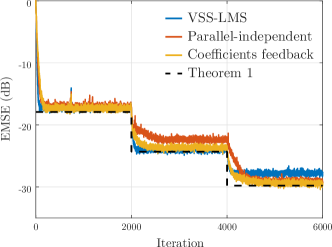
Beyond its conceptual value, (10) also provides a viable alternative to step size adaptation rules such as [4, 3, 6, 5]. Numerical experiments using combinations of LMS filters with cyclic coefficients feedback show that the resulting VSS algorithms are robust to changes in the environment and can track the optimal step-size even in stringent nonstationary scenarios (e.g., see Fig. 9).

It is worth noting that step size adaptation is only one possible application of coefficients feedback. In fact, these combinations are only related to VSS algorithms when all the AFs in the pool use the same adaptation algorithm and feedback occurs at every iteration. Combinations with cyclic coefficients feedback are therefore more general structures.
Refer to caption
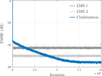
Figure 6: Steady-state of combination of LMS filters with cyclic coefficients feedback: EMSE performance. White stationary scenario (see Section VI): M=10𝑀10M=10, σu2=1superscriptsubscript𝜎𝑢21\sigma_{u}^{2}=1, σv2=103superscriptsubscript𝜎𝑣2superscript103\sigma_{v}^{2}=10^{-3}, μ1=0.01subscript𝜇10.01\mu_{1}=0.01, μ2=0.002subscript𝜇20.002\mu_{2}=0.002, and L=20𝐿20L=20. Affine supervisor: μη=1.5subscript𝜇𝜂1.5\mu_{\eta}=1.5 and η0.25μ¯0𝜂0.25¯𝜇0\eta\geq-0.25\Rightarrow\bar{\mu}\geq 0.

IV Steady-State and Tracking Performance

We begin the analysis of combinations of LMS filters with coefficients feedback by studying their steady-state performance in a system identification scenario. Although AFs can be used in a myriad of setups, their analyses are typically carried out in this setting as it is representative of applications such as echo cancellation, time delay estimation, and adaptive control [1, 2, 31, 32, 33]. Let 𝒖isubscript𝒖𝑖\bm{u}_{i} be a M×1𝑀1M\times 1 real-valued regressor vector with covariance matrix 𝑹u=𝔼𝒖i𝒖iTsubscript𝑹𝑢𝔼subscript𝒖𝑖superscriptsubscript𝒖𝑖𝑇\bm{R}_{u}=\operatorname{\mathbb{E}}\bm{u}_{i}\bm{u}_{i}^{T} and let d(i)𝑑𝑖d(i) be a scalar measurement of the form

d(i)=𝒖iT𝒘io+v(i),𝑑𝑖superscriptsubscript𝒖𝑖𝑇subscriptsuperscript𝒘𝑜𝑖𝑣𝑖,d(i)=\bm{u}_{i}^{T}\bm{w}^{o}_{i}+v(i)\text{,} (11)

where 𝒘ioMsubscriptsuperscript𝒘𝑜𝑖superscript𝑀\bm{w}^{o}_{i}\in\mathbb{R}^{M} represents the unknown system at iteration i𝑖i and v(i)𝑣𝑖v(i) is a zero-mean white Gaussian noise with variance σv2superscriptsubscript𝜎𝑣2\sigma_{v}^{2}. The system coefficients 𝒘iosubscriptsuperscript𝒘𝑜𝑖\bm{w}^{o}_{i} follow the first-order Markov process

𝒘io=𝒘i1o+𝒒i,subscriptsuperscript𝒘𝑜𝑖subscriptsuperscript𝒘𝑜𝑖1subscript𝒒𝑖,\bm{w}^{o}_{i}=\bm{w}^{o}_{i-1}+\bm{q}_{i}\text{,} (12)

where 𝒘1o=𝒘osubscriptsuperscript𝒘𝑜1superscript𝒘𝑜\bm{w}^{o}_{-1}=\bm{w}^{o} is the initial condition and 𝒒iMsubscript𝒒𝑖superscript𝑀\bm{q}_{i}\in\mathbb{R}^{M} is a zero-mean i.i.d. sequence of vectors with covariance matrix 𝑸=𝔼𝒒i𝒒iT𝑸𝔼subscript𝒒𝑖superscriptsubscript𝒒𝑖𝑇\bm{Q}=\operatorname{\mathbb{E}}\bm{q}_{i}\bm{q}_{i}^{T}. The stationary case is recovered for 𝒒i=𝟎𝑸=𝟎subscript𝒒𝑖0𝑸0\bm{q}_{i}=\bm{0}\Rightarrow\bm{Q}=\bm{0}. To make the derivations more tractable, we adopt the following typical assumptions [1, 2]:

A.1 (Noise independence)

{u(i),v(j)}𝑢𝑖𝑣𝑗\{u(i),v(j)\} are independent for all i,j𝑖𝑗i,j.

A.2 (Random walk independence)

The random variable 𝒒isubscript𝒒𝑖\bm{q}_{i} is statistically independent of the initial conditions {𝒘1o,𝒘n,1}subscriptsuperscript𝒘𝑜1subscript𝒘𝑛1\{\bm{w}^{o}_{-1},\bm{w}_{n,-1}\}, of {𝒖j,v(j)}subscript𝒖𝑗𝑣𝑗\{\bm{u}_{j},v(j)\} for all i,j𝑖𝑗i,j, and of {d(j)}𝑑𝑗\{d(j)\} for j<i𝑗𝑖j<i.

Our performance metric of interest is the excess MSE (EMSE) defined as follows. Let 𝒘~i=𝒘io𝒘isubscript~𝒘𝑖subscriptsuperscript𝒘𝑜𝑖subscript𝒘𝑖\widetilde{\bm{w}}_{i}=\bm{w}^{o}_{i}-\bm{w}_{i} and 𝒘~n,i=𝒘io𝒘n,isubscript~𝒘𝑛𝑖subscriptsuperscript𝒘𝑜𝑖subscript𝒘𝑛𝑖\widetilde{\bm{w}}_{n,i}=\bm{w}^{o}_{i}-\bm{w}_{n,i} be the global and local coefficient error vectors respectively. Define the global a priori error as ea(i)=𝒖iT(𝒘io𝒘i1)subscript𝑒𝑎𝑖superscriptsubscript𝒖𝑖𝑇subscriptsuperscript𝒘𝑜𝑖subscript𝒘𝑖1e_{a}(i)=\bm{u}_{i}^{T}(\bm{w}^{o}_{i}-\bm{w}_{i-1}) and its local counterpart as ea,n(i)=𝒖iT(𝒘io𝒘n,i1)subscript𝑒𝑎𝑛𝑖superscriptsubscript𝒖𝑖𝑇subscriptsuperscript𝒘𝑜𝑖subscript𝒘𝑛𝑖1e_{a,n}(i)=\bm{u}_{i}^{T}(\bm{w}^{o}_{i}-\bm{w}_{n,i-1}). For a combination of two filters, we then have

ζ(i)𝜁𝑖\displaystyle\zeta(i) =𝔼ea2(i)absent𝔼superscriptsubscript𝑒𝑎2𝑖\displaystyle=\operatorname{\mathbb{E}}e_{a}^{2}(i) (global EMSE) (13)
ζn(i)subscript𝜁𝑛𝑖\displaystyle\zeta_{n}(i) =𝔼ea,n2(i), for n=1,2formulae-sequenceabsent𝔼superscriptsubscript𝑒𝑎𝑛2𝑖, for 𝑛12\displaystyle=\operatorname{\mathbb{E}}e_{a,n}^{2}(i)\text{, for }n=1,2 (local EMSE)
ζ12(i)subscript𝜁12𝑖\displaystyle\zeta_{12}(i) =𝔼ea,1(i)ea,2(i)absent𝔼subscript𝑒𝑎1𝑖subscript𝑒𝑎2𝑖\displaystyle=\operatorname{\mathbb{E}}e_{a,1}(i)e_{a,2}(i) (cross-EMSE)
Refer to caption
Figure 7: Steady-state of combination of LMS filters with cyclic coefficients feedback: equivalent step-size of combination (same setting as Fig. 6).

Before proceeding, we derive some relations that will be useful throughout our analysis. First, subtract the global coefficients (5) from 𝒘iosubscriptsuperscript𝒘𝑜𝑖\bm{w}^{o}_{i} to get

𝒘~i=η(i)𝒘~1,i+[1η(i)]𝒘~2,i.subscript~𝒘𝑖𝜂𝑖subscript~𝒘1𝑖delimited-[]1𝜂𝑖subscript~𝒘2𝑖.\widetilde{\bm{w}}_{i}=\eta(i)\widetilde{\bm{w}}_{1,i}+\left[1-\eta(i)\right]\widetilde{\bm{w}}_{2,i}\text{.} (14)

Also, subtracting 𝒘iosubscriptsuperscript𝒘𝑜𝑖\bm{w}^{o}_{i} from (5) at i1𝑖1i-1 and multiplying by 𝒖iTsuperscriptsubscript𝒖𝑖𝑇\bm{u}_{i}^{T} yields

ea(i)=η(i1)ea,1(i)+[1η(i1)]ea,2(i).subscript𝑒𝑎𝑖𝜂𝑖1subscript𝑒𝑎1𝑖delimited-[]1𝜂𝑖1subscript𝑒𝑎2𝑖.e_{a}(i)=\eta(i-1)e_{a,1}(i)+\left[1-\eta(i-1)\right]e_{a,2}(i)\text{.} (15)

Using the definition of the component filters output, we obtain

y1(i)y2(i)=𝒖iT𝒘1,i1𝒖iT𝒘2,i1=ea,2(i)ea,1(i),subscript𝑦1𝑖subscript𝑦2𝑖superscriptsubscript𝒖𝑖𝑇subscript𝒘1𝑖1superscriptsubscript𝒖𝑖𝑇subscript𝒘2𝑖1subscript𝑒𝑎2𝑖subscript𝑒𝑎1𝑖,y_{1}(i)-y_{2}(i)=\bm{u}_{i}^{T}\bm{w}_{1,i-1}-\bm{u}_{i}^{T}\bm{w}_{2,i-1}=e_{a,2}(i)-e_{a,1}(i)\text{,} (16)

by adding and subtracting 𝒖iT𝒘iosuperscriptsubscript𝒖𝑖𝑇subscriptsuperscript𝒘𝑜𝑖\bm{u}_{i}^{T}\bm{w}^{o}_{i}. Finally, we can use (11) to write the global estimation error e(i)𝑒𝑖e(i) in terms of the a priori error as

e(i)𝑒𝑖\displaystyle e(i) =d(i)𝒖iT𝒘i1absent𝑑𝑖superscriptsubscript𝒖𝑖𝑇subscript𝒘𝑖1\displaystyle=d(i)-\bm{u}_{i}^{T}\bm{w}_{i-1} (17)
=𝒖iT𝒘io+v(i)𝒖iT𝒘i1=ea(i)+v(i).absentsuperscriptsubscript𝒖𝑖𝑇subscriptsuperscript𝒘𝑜𝑖𝑣𝑖superscriptsubscript𝒖𝑖𝑇subscript𝒘𝑖1subscript𝑒𝑎𝑖𝑣𝑖.\displaystyle=\bm{u}_{i}^{T}\bm{w}^{o}_{i}+v(i)-\bm{u}_{i}^{T}\bm{w}_{i-1}=e_{a}(i)+v(i)\text{.}

Note from (17) that under A.1 the global MSE is given by 𝔼e(i)2=ζ(i)+σv2𝔼𝑒superscript𝑖2𝜁𝑖superscriptsubscript𝜎𝑣2\operatorname{\mathbb{E}}e(i)^{2}=\zeta(i)+\sigma_{v}^{2}. Hence, although we carry out all derivations for the EMSE, our results can readily be used to measure performance with respect to the MSE.

We are now ready to state the main result of this section.

Theorem 1.

Consider the system identification scenario in (11)–(12) and a supervisor of the form (6). Under assumptions A.1–A.6, the steady-state value of the global EMSE of a combination of LMS filters with coefficients feedback is

ζ=μ¯Tr(𝑹u)σv2+μ¯1Tr(𝑸)2μ¯Tr(𝑹u),𝜁¯𝜇Trsubscript𝑹𝑢superscriptsubscript𝜎𝑣2superscript¯𝜇1Tr𝑸2¯𝜇Trsubscript𝑹𝑢,\zeta=\frac{\bar{\mu}\operatorname{Tr}(\bm{R}_{u})\sigma_{v}^{2}+\bar{\mu}^{-1}\operatorname{Tr}(\bm{Q})}{2-\bar{\mu}\operatorname{Tr}(\bm{R}_{u})}\text{,} (18)

where μ¯=η¯μ1+(1η¯)μ2¯𝜇¯𝜂subscript𝜇11¯𝜂subscript𝜇2\bar{\mu}=\bar{\eta}\mu_{1}+(1-\bar{\eta})\mu_{2}, η¯¯𝜂\bar{\eta} is the restriction of ηosuperscript𝜂𝑜\eta^{o} onto [f(a),f(a+)]𝑓superscript𝑎𝑓superscript𝑎[f(a^{-}),f(a^{+})], and

ηo=cTr(𝑹u)[Tr(𝑸)+2μ2σv2]2(μ1μ2)Tr(𝑹u)σv2,superscript𝜂𝑜𝑐Trsubscript𝑹𝑢delimited-[]Tr𝑸2subscript𝜇2superscriptsubscript𝜎𝑣22subscript𝜇1subscript𝜇2Trsubscript𝑹𝑢superscriptsubscript𝜎𝑣2,\eta^{o}=\frac{c-\operatorname{Tr}(\bm{R}_{u})\left[\operatorname{Tr}(\bm{Q})+2\mu_{2}\sigma_{v}^{2}\right]}{2(\mu_{1}-\mu_{2})\operatorname{Tr}(\bm{R}_{u})\sigma_{v}^{2}}\text{,} (19)

with c2=Tr(𝐑u)2Tr(𝐐)2+4σv2Tr(𝐑u)Tr(𝐐)c^{2}=\operatorname{Tr}(\bm{R}_{u})^{2}\operatorname{Tr}(\bm{Q})^{2}+4\sigma_{v}^{2}\operatorname{Tr}(\bm{R}_{u})\operatorname{Tr}(\bm{Q}) is the supervising parameter that minimizes the global MSE.

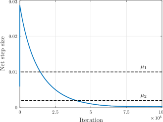
Given the relation between combinations with coefficients feedback and VSS algorithms, it is not surprising that (18) is equivalent to the expression for the steady-state of a standalone LMS filter with step size μ¯¯𝜇\bar{\mu} [1, Lemma 7.5.1]. Theorem 1, however, also states that μ¯¯𝜇\bar{\mu} is chosen by the supervisor to minimize the global MSE (see Proposition 2). In the nonstationary case, coefficients feedback therefore force the supervisor to explicitly track the optimal step size μosuperscript𝜇𝑜\mu^{o} from [1, Lemma 7.5.1]. For convex or affine supervisors, it then suffices that μ1μoμ2subscript𝜇1superscript𝜇𝑜subscript𝜇2\mu_{1}\leq\mu^{o}\leq\mu_{2} for the coefficients feedback topology to outperform any parallel-independent combination that does not have at least one component filter with step size μosuperscript𝜇𝑜\mu^{o}. Even if it does, recall that μosuperscript𝜇𝑜\mu^{o} depends on 𝑹usubscript𝑹𝑢\bm{R}_{u}, 𝑸𝑸\bm{Q}, and σv2superscriptsubscript𝜎𝑣2\sigma_{v}^{2}, so that parallel-independent combinations would not robust to changes in the environment. The adaptive step size effect of coefficients feedback, however, mitigates this issue.

Theorem 1 may no longer be valid in stationary scenarios, especially if the range of the activation function f𝑓f from (6) is unbounded, e.g., for the affine supervisor (7). In this case, 𝑸=𝟎𝑸0\bm{Q}=\bm{0} implies that ηoμ2(μ1μ2)1superscript𝜂𝑜subscript𝜇2superscriptsubscript𝜇1subscript𝜇21\eta^{o}\to\mu_{2}(\mu_{1}-\mu_{2})^{-1} and μ¯0¯𝜇0\bar{\mu}\to 0 at steady-state. However, Figs. 6 and 7 illustrates that, although μ¯¯𝜇\bar{\mu} and the EMSE decrease considerably, they both converge to a non-vanishing steady-state. This occurs because as the EMSE diminishes, the variance of the supervising parameter becomes non-negligible, violating the approximations used to derive Theorem 1. Nevertheless, Theorem 1 holds for the convex supervisor or any other case in which [f(a),f(a+)]𝑓superscript𝑎𝑓superscript𝑎[f(a^{-}),f(a^{+})] does not allow μ¯¯𝜇\bar{\mu} to vanish. Otherwise, we can resort to the transient analysis in Section V.

The remainder of this section is dedicated to proving Theorem 1. We proceed in three steps. First, we introduce the different steady-state regimes of the cyclic coefficients feedback topology and argue that for small cycle periods the combination performs as if L=1𝐿1L=1 (Section IV-A). Then, we derive the component filters error statistics required to obtain (18) (Section IV-B) and determine the steady-state value of the supervising parameter (Section IV-C). Recall that even though all derivations are carried out for two component filters, the results can be extended to arbitrary N𝑁N by evaluating additional error statistics or using hierarchical combinations [14, 15].

IV-A Global steady-state analysis

Analyzing the asymptotic performance of combinations with cyclic coefficients feedback is intricate due to the dynamic nature of their steady-state. Indeed, for cycle periods 1<L<1𝐿1<L<\infty, their topology alternates between parallel-independent and parallel with coefficients feedback, so that the component filters and the output of the combination reach a cyclostationary regime as i𝑖i\to\infty, as illustrated in Fig. 3b. In contrast, the limit cases L𝐿L\to\infty and L=1𝐿1L=1 have static topologies and stationary steady-state errors (Figs. 3a and 3c respectively). To account for cyclic feedback without resorting to a full transient analysis as in Section V, we leverage the fact that since feedbacks are cyclical solely to avoid stalling the supervisor adaptation, we care only about performance for small L𝐿L. Hence, we can use the following approximation, is valid for a significant range of L𝐿L (Figs. 4 and 5):

A.3 (Small cycle period)

For small cycle period, the combination performs at steady-state as if L=1𝐿1L=1.

Moreover, we can decouple the analysis of the global error and the supervisor by assuming that

A.4 (Steady-state supervisor separation principle)

At steady-state, η(i)𝜂𝑖\eta(i) varies slowly compared to the coefficients error vector 𝒘~n,isubscript~𝒘𝑛𝑖\widetilde{\bm{w}}_{n,i} and the a priori errors ea,n(i)subscript𝑒𝑎𝑛𝑖e_{a,n}(i), so that their expected values can be separated as in 𝔼[η(i)𝒘~n,i]=𝔼η(i)𝔼𝒘~n,i𝔼𝜂𝑖subscript~𝒘𝑛𝑖𝔼𝜂𝑖𝔼subscript~𝒘𝑛𝑖\operatorname{\mathbb{E}}[\eta(i)\widetilde{\bm{w}}_{n,i}]=\operatorname{\mathbb{E}}\eta(i)\operatorname{\mathbb{E}}\widetilde{\bm{w}}_{n,i} and 𝔼[η(i)ea,n(i)]=𝔼η(i)𝔼ea,n(i)𝔼𝜂𝑖subscript𝑒𝑎𝑛𝑖𝔼𝜂𝑖𝔼subscript𝑒𝑎𝑛𝑖\operatorname{\mathbb{E}}[\eta(i)e_{a,n}(i)]=\operatorname{\mathbb{E}}\eta(i)\operatorname{\mathbb{E}}e_{a,n}(i), i𝑖i\to\infty.

This assumption is supported by simulations and has been successfully used in the steady-state analysis of parallel-independent topologies, i.e., L𝐿L\to\infty, for both affine [12, 24, 27] and convex [10, 13] supervisors. Using A.4, we can now derive the result of Theorem 1 in two parts, by first analyzing the component filters and then the supervisor.

IV-B Component filters steady-state analysis

Start by taking the expected value of the squared norm of the coefficient error vector (14) to get

𝔼𝒘~i2𝔼superscriptnormsubscript~𝒘𝑖2\displaystyle\operatorname{\mathbb{E}}\left\|\widetilde{\bm{w}}_{i}\right\|^{2} =𝔼η2(i)𝒘~1,i2+2𝔼η(i)[1η(i)]𝒘~1,iT𝒘~2,iabsent𝔼superscript𝜂2𝑖superscriptnormsubscript~𝒘1𝑖22𝔼𝜂𝑖delimited-[]1𝜂𝑖superscriptsubscript~𝒘1𝑖𝑇subscript~𝒘2𝑖\displaystyle=\operatorname{\mathbb{E}}\eta^{2}(i)\left\|\widetilde{\bm{w}}_{1,i}\right\|^{2}+2\operatorname{\mathbb{E}}\eta(i)[1-\eta(i)]\widetilde{\bm{w}}_{1,i}^{T}\widetilde{\bm{w}}_{2,i}
+𝔼[1η(i)]2𝒘~2,i2.\displaystyle+\operatorname{\mathbb{E}}[1-\eta(i)]^{2}\left\|\widetilde{\bm{w}}_{2,i}\right\|^{2}\text{.}

Then, using A.4, we can separate the expectations and obtain

𝔼𝒘~i2𝔼superscriptnormsubscript~𝒘𝑖2\displaystyle\operatorname{\mathbb{E}}\left\|\widetilde{\bm{w}}_{i}\right\|^{2} =𝔼η2𝔼𝒘~1,i2+2𝔼η[1η]𝔼𝒘~1,iT𝒘~2,iabsent𝔼superscript𝜂2𝔼superscriptnormsubscript~𝒘1𝑖22𝔼𝜂delimited-[]1𝜂𝔼superscriptsubscript~𝒘1𝑖𝑇subscript~𝒘2𝑖\displaystyle=\operatorname{\mathbb{E}}\eta^{2}\operatorname{\mathbb{E}}\left\|\widetilde{\bm{w}}_{1,i}\right\|^{2}+2\operatorname{\mathbb{E}}\eta[1-\eta]\operatorname{\mathbb{E}}\widetilde{\bm{w}}_{1,i}^{T}\widetilde{\bm{w}}_{2,i} (20)
+𝔼[1η]2𝔼𝒘~2,i2,as i.\displaystyle+\operatorname{\mathbb{E}}[1-\eta]^{2}\operatorname{\mathbb{E}}\left\|\widetilde{\bm{w}}_{2,i}\right\|^{2}\text{,}\quad\text{as }i\to\infty\text{.}

The component filters error statistics required in (20) can be evaluated using an energy conservation argument as in [1]. We do so by adopting the following assumption to derive the variance and covariance relations of the AFs in the combination.

A.5 (Data separation principle)

𝒖i2superscriptnormsubscript𝒖𝑖2\left\|\bm{u}_{i}\right\|^{2} is independent of ea,n(i)subscript𝑒𝑎𝑛𝑖e_{a,n}(i), and consequently ea(i)subscript𝑒𝑎𝑖e_{a}(i), at steady-state.

We then have the following proposition:

Proposition 1.

Under A.1, A.2, and A.5, the variance and covariance relations for the LMS component filters of a combination with coefficients feedback (L=1𝐿1L=1) are given by

𝔼𝒘~n,i2𝔼superscriptnormsubscript~𝒘𝑛𝑖2\displaystyle\operatorname{\mathbb{E}}\left\|\widetilde{\bm{w}}_{n,i}\right\|^{2} =𝔼𝒘~i12+Tr(𝑸)absent𝔼superscriptnormsubscript~𝒘𝑖12Tr𝑸\displaystyle=\operatorname{\mathbb{E}}\left\|\widetilde{\bm{w}}_{i-1}\right\|^{2}+\operatorname{Tr}(\bm{Q})
2μnζ(i)+μn2Tr(𝑹u)[ζ(i)+σv2],2subscript𝜇𝑛𝜁𝑖superscriptsubscript𝜇𝑛2Trsubscript𝑹𝑢delimited-[]𝜁𝑖superscriptsubscript𝜎𝑣2,\displaystyle-2\mu_{n}\zeta(i)+\mu_{n}^{2}\operatorname{Tr}(\bm{R}_{u})\left[\zeta(i)+\sigma_{v}^{2}\right]\text{,} (21a)
𝔼𝒘~1,iT𝒘~2,i𝔼superscriptsubscript~𝒘1𝑖𝑇subscript~𝒘2𝑖\displaystyle\operatorname{\mathbb{E}}\widetilde{\bm{w}}_{1,i}^{T}\widetilde{\bm{w}}_{2,i} =𝔼𝒘~i12+Tr(𝑸)(μ1+μ2)ζ(i)absent𝔼superscriptnormsubscript~𝒘𝑖12Tr𝑸subscript𝜇1subscript𝜇2𝜁𝑖\displaystyle=\operatorname{\mathbb{E}}\left\|\widetilde{\bm{w}}_{i-1}\right\|^{2}+\operatorname{Tr}(\bm{Q})-(\mu_{1}+\mu_{2})\zeta(i)
+μ1μ2Tr(𝑹u)[ζ(i)+σv2],subscript𝜇1subscript𝜇2Trsubscript𝑹𝑢delimited-[]𝜁𝑖superscriptsubscript𝜎𝑣2,\displaystyle+\mu_{1}\mu_{2}\operatorname{Tr}(\bm{R}_{u})\left[\zeta(i)+\sigma_{v}^{2}\right]\text{,} (21b)

as i𝑖i\to\infty.

Proof.

See Appendix A. ∎

Note that, as opposed to the analysis of parallel-independent combinations [10, 12, 24], the recursions in (21) are coupled. Substituting (21) into the steady-state relation (20) gives

𝔼𝒘~i2𝔼superscriptnormsubscript~𝒘𝑖2\displaystyle\operatorname{\mathbb{E}}\left\|\widetilde{\bm{w}}_{i}\right\|^{2} =𝔼𝒘~i12+Tr(𝑸)2𝔼μ^ζ(i)absent𝔼superscriptnormsubscript~𝒘𝑖12Tr𝑸2𝔼^𝜇𝜁𝑖\displaystyle=\operatorname{\mathbb{E}}\left\|\widetilde{\bm{w}}_{i-1}\right\|^{2}+\operatorname{Tr}(\bm{Q})-2\operatorname{\mathbb{E}}\hat{\mu}\zeta(i) (22)
+𝔼μ^2Tr(𝑹u)[ζ(i)+σv2], as i,𝔼superscript^𝜇2Trsubscript𝑹𝑢delimited-[]𝜁𝑖superscriptsubscript𝜎𝑣2, as 𝑖,\displaystyle+\operatorname{\mathbb{E}}\hat{\mu}^{2}\operatorname{Tr}(\bm{R}_{u})\left[\zeta(i)+\sigma_{v}^{2}\right]\text{, as }i\to\infty\text{,}

where μ^=ημ1+[1η]μ2^𝜇𝜂subscript𝜇1delimited-[]1𝜂subscript𝜇2\hat{\mu}=\eta\mu_{1}+[1-\eta]\mu_{2} is the steady-state net step size of the combination with η=limiη(i)𝜂subscript𝑖𝜂𝑖\eta=\lim_{i\to\infty}\eta(i). Note that μ^^𝜇\hat{\mu} is a random variable due to its dependence on η𝜂\eta.

To conclude the component analysis, recall that under A.3 we only consider the L=1𝐿1L=1 case in which the combination topology is static. Hence, 𝔼𝒘~i2𝔼superscriptnormsubscript~𝒘𝑖2\operatorname{\mathbb{E}}\left\|\widetilde{\bm{w}}_{i}\right\|^{2} eventually converges to a stationary value for a proper choice of μ1subscript𝜇1\mu_{1} and μ2subscript𝜇2\mu_{2}, and 𝔼𝒘~i2=𝔼𝒘~i12𝔼superscriptnormsubscript~𝒘𝑖2𝔼superscriptnormsubscript~𝒘𝑖12\operatorname{\mathbb{E}}\left\|\widetilde{\bm{w}}_{i}\right\|^{2}=\operatorname{\mathbb{E}}\left\|\widetilde{\bm{w}}_{i-1}\right\|^{2} as i𝑖i\to\infty. We can therefore rewrite (22) as

𝔼μ^2Tr(𝑹u)[ζ+σv2]+Tr(𝑸)=2𝔼μ^ζ.𝔼superscript^𝜇2Trsubscript𝑹𝑢delimited-[]𝜁superscriptsubscript𝜎𝑣2Tr𝑸2𝔼^𝜇𝜁.\operatorname{\mathbb{E}}\hat{\mu}^{2}\operatorname{Tr}(\bm{R}_{u})\left[\zeta+\sigma_{v}^{2}\right]+\operatorname{Tr}(\bm{Q})=2\operatorname{\mathbb{E}}\hat{\mu}\zeta\text{.} (23)

Recall that ζ𝜁\zeta is the steady-state value of the EMSE ζ(i)𝜁𝑖\zeta(i). All that remains to obtain (18) is to determine the supervisor moments needed to evaluate (23).

IV-C Supervisor steady-state analysis

To analyze the steady-state value of the supervising parameter we adopt the following typical assumption [12, 24, 27, 10, 13]:

A.6 (Small variance assumption)

The variance of η(i)𝜂𝑖\eta(i) becomes negligible as i𝑖i\to\infty, so that 𝔼η2(i)[𝔼η(i)]2𝔼superscript𝜂2𝑖superscriptdelimited-[]𝔼𝜂𝑖2\operatorname{\mathbb{E}}\eta^{2}(i)\approx[\operatorname{\mathbb{E}}\eta(i)]^{2}.

Immediately, (23) becomes

μ¯Tr(𝑹u)[ζ+σv2]+Tr(𝑸)=2μ¯ζ,¯𝜇Trsubscript𝑹𝑢delimited-[]𝜁superscriptsubscript𝜎𝑣2Tr𝑸2¯𝜇𝜁,\bar{\mu}\operatorname{Tr}(\bm{R}_{u})\left[\zeta+\sigma_{v}^{2}\right]+\operatorname{Tr}(\bm{Q})=2\bar{\mu}\zeta\text{,} (24)

recalling that μ¯=η¯μ1+(1η¯)μ2¯𝜇¯𝜂subscript𝜇11¯𝜂subscript𝜇2\bar{\mu}=\bar{\eta}\mu_{1}+(1-\bar{\eta})\mu_{2} with η¯=limi𝔼η(i)¯𝜂subscript𝑖𝔼𝜂𝑖\bar{\eta}=\lim_{i\to\infty}\operatorname{\mathbb{E}}\eta(i). It is ready that (24) can be rearranged as in (18).

To obtain η¯¯𝜂\bar{\eta}, notice from (20) that the mean supervising parameter must converge to a fixed value for the combination to reach global steady-state, i.e., for 𝔼𝒘~i2=𝔼𝒘~i12𝔼superscriptnormsubscript~𝒘𝑖2𝔼superscriptnormsubscript~𝒘𝑖12\operatorname{\mathbb{E}}\left\|\widetilde{\bm{w}}_{i}\right\|^{2}=\operatorname{\mathbb{E}}\left\|\widetilde{\bm{w}}_{i-1}\right\|^{2}. In other words, η¯¯𝜂\bar{\eta} in (24) must be a fixed point of the expected value of (6). We characterize this fixed point in the following proposition.

Proposition 2.

Let ηoargminηζsuperscript𝜂𝑜subscriptargmin𝜂𝜁\eta^{o}\in\operatorname*{argmin}_{\eta}\zeta denote a supervising parameter that minimizes the steady-state global EMSE and ηsuperscript𝜂\eta^{\star} be a fixed point of the expected value of (6). Under A.1, A.2, and A.4, if ηo[f(a),f(a+)]superscript𝜂𝑜𝑓superscript𝑎𝑓superscript𝑎\eta^{o}\in[f(a^{-}),f(a^{+})], then η=ηosuperscript𝜂superscript𝜂𝑜\eta^{\star}=\eta^{o}.

Proof.

See Appendix B. ∎

Proposition 2 states that, unless constrained by the activation function, the fixed point of the mean supervising parameter update minimizes the global MSE. Hence, we can approximate the mean steady-state value of the supervising parameters by minimizing the steady-state EMSE expression (18) and projecting the minimum onto the range of f𝑓f. Similar approximations were used in the steady-state analysis of parallel-independent combinations [10, 12, 34].

Explicitly, the minimum of (18) is obtained when

ζη¯𝜁¯𝜂\displaystyle\frac{\partial\zeta}{\partial\bar{\eta}} =Tr(𝑹u)σv2(μ1μ2)2η¯2absentTrsubscript𝑹𝑢superscriptsubscript𝜎𝑣2superscriptsubscript𝜇1subscript𝜇22superscript¯𝜂2\displaystyle=\operatorname{Tr}(\bm{R}_{u})\sigma_{v}^{2}(\mu_{1}-\mu_{2})^{2}\bar{\eta}^{2} (25)
+Tr(𝑹u)[Tr(𝑸)+2μ2σv2](μ1μ2)η¯Trsubscript𝑹𝑢delimited-[]Tr𝑸2subscript𝜇2superscriptsubscript𝜎𝑣2subscript𝜇1subscript𝜇2¯𝜂\displaystyle+\operatorname{Tr}(\bm{R}_{u})\left[\operatorname{Tr}(\bm{Q})+2\mu_{2}\sigma_{v}^{2}\right](\mu_{1}-\mu_{2})\bar{\eta}
+Tr(𝑹u)σv2μ22+Tr(𝑹u)Tr(𝑸)μ2Tr(𝑸)=0.Trsubscript𝑹𝑢superscriptsubscript𝜎𝑣2superscriptsubscript𝜇22Trsubscript𝑹𝑢Tr𝑸subscript𝜇2Tr𝑸0.\displaystyle+\operatorname{Tr}(\bm{R}_{u})\sigma_{v}^{2}\mu_{2}^{2}+\operatorname{Tr}(\bm{R}_{u})\operatorname{Tr}(\bm{Q})\mu_{2}-\operatorname{Tr}(\bm{Q})=0\text{.}

Taking ηosuperscript𝜂𝑜\eta^{o} to be the root of (25) such that the net step size ηoμ1+(1ηo)μ20superscript𝜂𝑜subscript𝜇11superscript𝜂𝑜subscript𝜇20\eta^{o}\mu_{1}+(1-\eta^{o})\mu_{2}\geq 0 yields (19) and concludes the proof of Theorem 1.

V Transient Performance

The performance analysis from Section IV show that coefficients feedback can be used to improve the steady-state and tracking of parallel combinations. Recall, however, that the initial motivation for this topology was addressing the convergence stagnation issue. In this section, we therefore examine the transient behavior of a combination of LMS filters with cyclic coefficients feedback and in doing so, study the impact of cyclic feedback on the supervisor variance. Although transient analyses of convex and affine supervising rules in parallel-independent topologies have been carried out [24, 25, 35, 27], the following derivations are valid for generic activation functions by extending the approach from [25].

In what follows, we consider a stationary system identification scenario, i.e., 𝒒i=0subscript𝒒𝑖0\bm{q}_{i}=0 in (12), so that the coefficient error vectors become 𝒘~i=𝒘o𝒘isubscript~𝒘𝑖superscript𝒘𝑜subscript𝒘𝑖\widetilde{\bm{w}}_{i}=\bm{w}^{o}-\bm{w}_{i} and 𝒘~n,i=𝒘o𝒘n,isubscript~𝒘𝑛𝑖superscript𝒘𝑜subscript𝒘𝑛𝑖\widetilde{\bm{w}}_{n,i}=\bm{w}^{o}-\bm{w}_{n,i} and the a priori errors can be written as ea(i)=𝒖i𝒘~i1subscript𝑒𝑎𝑖subscript𝒖𝑖subscript~𝒘𝑖1e_{a}(i)=\bm{u}_{i}\widetilde{\bm{w}}_{i-1} and ea,n(i)=𝒖i𝒘~n,i1subscript𝑒𝑎𝑛𝑖subscript𝒖𝑖subscript~𝒘𝑛𝑖1e_{a,n}(i)=\bm{u}_{i}\widetilde{\bm{w}}_{n,i-1}. We also need to strengthen some of the assumptions from Section IV. Namely,

A.7 (Input signal assumptions)

{𝒖i}subscript𝒖𝑖\{\bm{u}_{i}\} is an i.i.d. sequence of Gaussian vectors with covariance 𝑹usubscript𝑹𝑢\bm{R}_{u} and independent of v(j)𝑣𝑗v(j) for all i,j𝑖𝑗i,j. Consequently, {𝒖i,𝒘~j}subscript𝒖𝑖subscript~𝒘𝑗\{\bm{u}_{i},\widetilde{\bm{w}}_{j}\}, {d(i),d(j)}𝑑𝑖𝑑𝑗\{d(i),d(j)\}, and {𝒖i,d(j)}subscript𝒖𝑖𝑑𝑗\{\bm{u}_{i},d(j)\} are independent for i>j𝑖𝑗i>j.

A.8 (Transient supervisor separation principle)

The supervising parameter varies slowly enough that, for m,n=1,2formulae-sequence𝑚𝑛12m,n=1,2, 𝔼[η(i1)ea,m(i)ea,n(i)]=𝔼η(i1)𝔼[ea,m(i)ea,n(i)]𝔼𝜂𝑖1subscript𝑒𝑎𝑚𝑖subscript𝑒𝑎𝑛𝑖𝔼𝜂𝑖1𝔼subscript𝑒𝑎𝑚𝑖subscript𝑒𝑎𝑛𝑖\operatorname{\mathbb{E}}[\eta(i-1)e_{a,m}(i)e_{a,n}(i)]=\operatorname{\mathbb{E}}\eta(i-1)\operatorname{\mathbb{E}}[e_{a,m}(i)e_{a,n}(i)].

A.9 (Jointly Gaussian a priori errors)

The a priori error {ea,n(i)}subscript𝑒𝑎𝑛𝑖\{e_{a,n}(i)\}, n=1,2𝑛12n=1,2, are zero-mean jointly Gaussian random variables, so that

𝔼ea,n4(i)𝔼superscriptsubscript𝑒𝑎𝑛4𝑖\displaystyle\operatorname{\mathbb{E}}e_{a,n}^{4}(i) =3ζn2(i)absent3superscriptsubscript𝜁𝑛2𝑖\displaystyle=3\zeta_{n}^{2}(i)
𝔼ea,1k(i)ea,2(i)𝔼superscriptsubscript𝑒𝑎1𝑘𝑖superscriptsubscript𝑒𝑎2𝑖\displaystyle\operatorname{\mathbb{E}}e_{a,1}^{k}(i)e_{a,2}^{\ell}(i) ={0,k+=33ζ1(i)ζ12(i),k=3,=13ζ2(i)ζ12(i),k=1,=32ζ122(i)+ζ1(i)ζ2(i),k==2absentcases0,𝑘33subscript𝜁1𝑖subscript𝜁12𝑖,formulae-sequence𝑘313subscript𝜁2𝑖subscript𝜁12𝑖,formulae-sequence𝑘132superscriptsubscript𝜁122𝑖subscript𝜁1𝑖subscript𝜁2𝑖,𝑘2\displaystyle=\begin{cases}0\text{,}&k+\ell=3\\ 3\zeta_{1}(i)\zeta_{12}(i)\text{,}&k=3,\ell=1\\ 3\zeta_{2}(i)\zeta_{12}(i)\text{,}&k=1,\ell=3\\ 2\zeta_{12}^{2}(i)+\zeta_{1}(i)\zeta_{2}(i)\text{,}&k=\ell=2\end{cases}

Assumption A.7 is used to evaluate higher-order moments of the input signal. Although stronger than A.5, it is common in the transient analysis of standalone AFs [1, 2]. Note that, although the vector sequence {𝒖i}subscript𝒖𝑖\{\bm{u}_{i}\} is i.i.d., the elements within each vector 𝒖isubscript𝒖𝑖\bm{u}_{i} can be correlated. Additionally, assumption A.8 allows us to decouple the analysis of the component filters and the supervisor, and A.9 is used to evaluate moments of the a priori errors for the supervisor variance recursion.

The following theorem collects the complete transient analysis from this section.

Theorem 2.

Let 𝐑u=𝐔𝚲𝐔Tsubscript𝐑𝑢𝐔𝚲superscript𝐔𝑇\bm{R}_{u}=\bm{U}\bm{\Lambda}\bm{U}^{T} be the eigenvalue decomposition of the regressor covariance matrix. Also, let the component filters coefficient vectors and the supervising parameters be initialized as 𝐰n,1=𝟎subscript𝐰𝑛10\bm{w}_{n,-1}=\bm{0}, a¯(1)=0.5¯𝑎10.5\bar{a}(-1)=0.5, and σa2(1)=0superscriptsubscript𝜎𝑎210\sigma_{a}^{2}(-1)=0, so that 𝐊^n,1=𝐔T𝐰o(𝐰o)T𝐔subscriptbold-^𝐊𝑛1superscript𝐔𝑇superscript𝐰𝑜superscriptsuperscript𝐰𝑜𝑇𝐔\bm{{\hat{K}}}_{n,-1}=\bm{U}^{T}\bm{w}^{o}(\bm{w}^{o})^{T}\bm{U} and Δ𝐊^n,1=𝟎Δsubscriptbold-^𝐊𝑛10\Delta\bm{{\hat{K}}}_{n,-1}=\bm{0}. Then, under A.7–A.9, the EMSE at iteration i𝑖i can be computed recursively by the following steps

  1. (i)

    Evaluate the supervising parameter moments using

    𝔼η2(i1)𝔼superscript𝜂2𝑖1\displaystyle\operatorname{\mathbb{E}}\eta^{2}(i-1) f[a¯(i1)]2+σa2(i1)f[a¯(i1)]2absent𝑓superscriptdelimited-[]¯𝑎𝑖12superscriptsubscript𝜎𝑎2𝑖1superscript𝑓superscriptdelimited-[]¯𝑎𝑖12\displaystyle\approx f\left[\bar{a}(i-1)\right]^{2}+\sigma_{a}^{2}(i-1)f^{\prime}\left[\bar{a}(i-1)\right]^{2}
    𝔼η(i1)𝔼𝜂𝑖1\displaystyle\operatorname{\mathbb{E}}\eta(i-1) f[a¯(i1)]absent𝑓delimited-[]¯𝑎𝑖1\displaystyle\approx f\left[\bar{a}(i-1)\right]
  2. (ii)

    Evaluate the global EMSE using ζn(i)=Tr(𝚲𝑲^n,i1)subscript𝜁𝑛𝑖Tr𝚲subscriptbold-^𝑲𝑛𝑖1\zeta_{n}(i)=\operatorname{Tr}(\bm{\Lambda}\bm{{\hat{K}}}_{n,i-1}), Δζn(i)=Tr(𝚲Δ𝑲^n,i1)Δsubscript𝜁𝑛𝑖Tr𝚲Δsubscriptbold-^𝑲𝑛𝑖1\Delta\zeta_{n}(i)=\operatorname{Tr}(\bm{\Lambda}\Delta\bm{{\hat{K}}}_{n,i-1}), and

    ζ(i)𝜁𝑖\displaystyle\zeta(i) =[𝔼η2(i1)][Δζ1(i)+Δζ2(i)]absentdelimited-[]𝔼superscript𝜂2𝑖1delimited-[]Δsubscript𝜁1𝑖Δsubscript𝜁2𝑖\displaystyle=\left[\operatorname{\mathbb{E}}\eta^{2}(i-1)\right][\Delta\zeta_{1}(i)+\Delta\zeta_{2}(i)]
    2[𝔼η(i1)]Δζ2(i)+ζ2(i)2delimited-[]𝔼𝜂𝑖1Δsubscript𝜁2𝑖subscript𝜁2𝑖\displaystyle-2\left[\operatorname{\mathbb{E}}\eta(i-1)\right]\Delta\zeta_{2}(i)+\zeta_{2}(i)
  3. (iii)

    Update the error covariance matrices: {(26),i=rL(27),irLcases(26),𝑖𝑟𝐿(27),𝑖𝑟𝐿\displaystyle\begin{cases}\text{\eqref{E:FinalTrMSDFB1},}&i=rL\\ \text{\eqref{E:FinalTrMSDNoFB1},}&i\neq rL\end{cases}

  4. (iv)

    Update the supervisor statistics using

    a¯(i)¯𝑎𝑖\displaystyle\bar{a}(i) a¯(i1)+μa[(1f¯)Δζ2f¯Δζ1]f¯absent¯𝑎𝑖1subscript𝜇𝑎delimited-[]1¯𝑓Δsubscript𝜁2¯𝑓Δsubscript𝜁1superscript¯𝑓\displaystyle\approx\bar{a}(i-1)+\mu_{a}[(1-\bar{f})\Delta\zeta_{2}-\bar{f}\Delta\zeta_{1}]\bar{f}^{\prime}
    σa2(i)superscriptsubscript𝜎𝑎2𝑖\displaystyle\sigma_{a}^{2}(i) [1+2μaG1+μa2G2]σa2(i1)+μa2Gvabsentdelimited-[]12subscript𝜇𝑎subscript𝐺1superscriptsubscript𝜇𝑎2subscript𝐺2superscriptsubscript𝜎𝑎2𝑖1superscriptsubscript𝜇𝑎2subscript𝐺𝑣\displaystyle\approx\left[1+2\mu_{a}G_{1}+\mu_{a}^{2}G_{2}\right]\sigma_{a}^{2}(i-1)+\mu_{a}^{2}G_{v}

    for the G𝐺G defined in (44).

For m,n=1,2formulae-sequence𝑚𝑛12m,n=1,2 and mn𝑚𝑛m\neq n, the error covariance matrices are updated as

𝑲^n,isubscriptbold-^𝑲𝑛𝑖\displaystyle\bm{{\hat{K}}}_{n,i} =𝑲^i1μn[𝑲^i1𝚲+𝚲𝑲^i1]+μn2𝑨absentsubscriptbold-^𝑲𝑖1subscript𝜇𝑛delimited-[]subscriptbold-^𝑲𝑖1𝚲𝚲subscriptbold-^𝑲𝑖1superscriptsubscript𝜇𝑛2𝑨\displaystyle=\bm{{\hat{K}}}_{i-1}-\mu_{n}[\bm{{\hat{K}}}_{i-1}\bm{\Lambda}+\bm{\Lambda}\bm{{\hat{K}}}_{i-1}]+\mu_{n}^{2}\bm{A} (26)
Δ𝑲^n,iΔsubscriptbold-^𝑲𝑛𝑖\displaystyle\Delta\bm{{\hat{K}}}_{n,i} =(μmμn)(𝑲^i1𝚲μn𝑨)absentsubscript𝜇𝑚subscript𝜇𝑛subscriptbold-^𝑲𝑖1𝚲subscript𝜇𝑛𝑨\displaystyle=(\mu_{m}-\mu_{n})\left(\bm{{\hat{K}}}_{i-1}\bm{\Lambda}-\mu_{n}\bm{A}\right)

for i=rL𝑖𝑟𝐿i=rL and 𝐀=σv2𝚲+𝚲Tr(𝐊^i1𝚲)+2𝚲𝐊^i1𝚲𝐀superscriptsubscript𝜎𝑣2𝚲𝚲Trsubscriptbold-^𝐊𝑖1𝚲2𝚲subscriptbold-^𝐊𝑖1𝚲\bm{A}=\sigma_{v}^{2}\bm{\Lambda}+\bm{\Lambda}\operatorname{Tr}(\bm{{\hat{K}}}_{i-1}\bm{\Lambda})+2\bm{\Lambda}\bm{{\hat{K}}}_{i-1}\bm{\Lambda} or

𝑲^n,isubscriptbold-^𝑲𝑛𝑖\displaystyle\bm{{\hat{K}}}_{n,i} =𝑲^n,i1+μn2𝑨nabsentsubscriptbold-^𝑲𝑛𝑖1superscriptsubscript𝜇𝑛2subscript𝑨𝑛\displaystyle=\bm{{\hat{K}}}_{n,i-1}+\mu_{n}^{2}\bm{A}_{n} (27)
μn[𝑲^n,i1𝚲+𝚲𝑲^n,i1]subscript𝜇𝑛delimited-[]subscriptbold-^𝑲𝑛𝑖1𝚲𝚲subscriptbold-^𝑲𝑛𝑖1\displaystyle-\mu_{n}[\bm{{\hat{K}}}_{n,i-1}\bm{\Lambda}+\bm{\Lambda}\bm{{\hat{K}}}_{n,i-1}]
𝑲^12,isubscriptbold-^𝑲12𝑖\displaystyle\bm{{\hat{K}}}_{12,i} =𝑲^12,i1μ1𝚲𝑲^12,i1absentsubscriptbold-^𝑲12𝑖1subscript𝜇1𝚲subscriptbold-^𝑲12𝑖1\displaystyle=\bm{{\hat{K}}}_{12,i-1}-\mu_{1}\bm{\Lambda}\bm{{\hat{K}}}_{12,i-1}
μ2𝑲^12,i1𝚲+μ1μ2𝑨12.subscript𝜇2subscriptbold-^𝑲12𝑖1𝚲subscript𝜇1subscript𝜇2subscript𝑨12.\displaystyle-\mu_{2}\bm{{\hat{K}}}_{12,i-1}\bm{\Lambda}+\mu_{1}\mu_{2}\bm{A}_{12}\text{.}

for irL𝑖𝑟𝐿i\neq rL, 𝐀n=σv2𝚲+𝚲Tr(𝐊^n,i1𝚲)+2𝚲𝐊^n,i1𝚲subscript𝐀𝑛superscriptsubscript𝜎𝑣2𝚲𝚲Trsubscriptbold-^𝐊𝑛𝑖1𝚲2𝚲subscriptbold-^𝐊𝑛𝑖1𝚲\bm{A}_{n}=\sigma_{v}^{2}\bm{\Lambda}+\bm{\Lambda}\operatorname{Tr}(\bm{{\hat{K}}}_{n,i-1}\bm{\Lambda})+2\bm{\Lambda}\bm{{\hat{K}}}_{n,i-1}\bm{\Lambda}, and 𝐀12=σv2𝚲+2𝚲𝐊^12,i1𝚲+Tr(𝚲𝐊^12,i1)𝚲subscript𝐀12superscriptsubscript𝜎𝑣2𝚲2𝚲subscriptbold-^𝐊12𝑖1𝚲Tr𝚲subscriptbold-^𝐊12𝑖1𝚲\bm{A}_{12}=\sigma_{v}^{2}\bm{\Lambda}+2\bm{\Lambda}\bm{{\hat{K}}}_{12,i-1}\bm{\Lambda}+\operatorname{Tr}(\bm{\Lambda}\bm{{\hat{K}}}_{12,i-1})\bm{\Lambda}.

Although Theorem 2 presents our results in full generality, it is more straightforward to interpret these results when the input signal is white.

Corollary 1.

For white input signals, i.e., 𝐑u=σu2𝐈subscript𝐑𝑢superscriptsubscript𝜎𝑢2𝐈\bm{R}_{u}=\sigma_{u}^{2}\bm{I}, the recursions (26) and (27) reduce to

ζn(i)subscript𝜁𝑛𝑖\displaystyle\zeta_{n}(i) =anζ(i1)+μn2Mσu4σv2absentsubscript𝑎𝑛𝜁𝑖1superscriptsubscript𝜇𝑛2𝑀superscriptsubscript𝜎𝑢4superscriptsubscript𝜎𝑣2\displaystyle=a_{n}\zeta(i-1)+\mu_{n}^{2}M\sigma_{u}^{4}\sigma_{v}^{2} (28)
Δζn(i)Δsubscript𝜁𝑛𝑖\displaystyle\Delta\zeta_{n}(i) =(μmμn)σu2[bnζ(i1)+μnMσu2σv2]absentsubscript𝜇𝑚subscript𝜇𝑛superscriptsubscript𝜎𝑢2delimited-[]subscript𝑏𝑛𝜁𝑖1subscript𝜇𝑛𝑀superscriptsubscript𝜎𝑢2superscriptsubscript𝜎𝑣2\displaystyle=(\mu_{m}-\mu_{n})\sigma_{u}^{2}\left[b_{n}\zeta(i-1)+\mu_{n}M\sigma_{u}^{2}\sigma_{v}^{2}\right]

for i=rL𝑖𝑟𝐿i=rL and

ζn(i)subscript𝜁𝑛𝑖\displaystyle\zeta_{n}(i) =anζn(i1)+μn2Mσu4σv2absentsubscript𝑎𝑛subscript𝜁𝑛𝑖1superscriptsubscript𝜇𝑛2𝑀superscriptsubscript𝜎𝑢4superscriptsubscript𝜎𝑣2\displaystyle=a_{n}\zeta_{n}(i-1)+\mu_{n}^{2}M\sigma_{u}^{4}\sigma_{v}^{2} (29)
Δζn(i)Δsubscript𝜁𝑛𝑖\displaystyle\Delta\zeta_{n}(i) =[1μnσu2]Δζn(i1)absentdelimited-[]1subscript𝜇𝑛superscriptsubscript𝜎𝑢2Δsubscript𝜁𝑛𝑖1\displaystyle=[1-\mu_{n}\sigma_{u}^{2}]\Delta\zeta_{n}(i-1)
σu2bn[μnζn(i1)μmζ12(i1)]superscriptsubscript𝜎𝑢2subscript𝑏𝑛delimited-[]subscript𝜇𝑛subscript𝜁𝑛𝑖1subscript𝜇𝑚subscript𝜁12𝑖1\displaystyle-\sigma_{u}^{2}b_{n}[\mu_{n}\zeta_{n}(i-1)-\mu_{m}\zeta_{12}(i-1)]
+μn(μnμm)Mσu4σv2subscript𝜇𝑛subscript𝜇𝑛subscript𝜇𝑚𝑀superscriptsubscript𝜎𝑢4superscriptsubscript𝜎𝑣2\displaystyle+\mu_{n}(\mu_{n}-\mu_{m})M\sigma_{u}^{4}\sigma_{v}^{2}

for irL𝑖𝑟𝐿i\neq rL, an=12μnσu2+μn2(M+2)σu4subscript𝑎𝑛12subscript𝜇𝑛superscriptsubscript𝜎𝑢2superscriptsubscript𝜇𝑛2𝑀2superscriptsubscript𝜎𝑢4a_{n}=1-2\mu_{n}\sigma_{u}^{2}+\mu_{n}^{2}(M+2)\sigma_{u}^{4}, and bn=1μn(M+2)σu2subscript𝑏𝑛1subscript𝜇𝑛𝑀2superscriptsubscript𝜎𝑢2b_{n}=1-\mu_{n}(M+2)\sigma_{u}^{2}.

Theorem 2 and Corollary 1 show the advantages of cyclic coefficients feedback from the viewpoint of convergence. Firstly, notice from (28) that the EMSE of both component filters are functions of the global EMSE upon feedback. As such, convergence stagnation is eradicated since the difference between the component errors cannot become too large for moderately sized cycle periods. Indeed, upon feedback, the difference between the ζn(i)subscript𝜁𝑛𝑖\zeta_{n}(i) is proportional to the difference between the component filters step sizes. Secondly, coefficients feedback reduces the EMSE/cross-EMSE gap, whose magnitude becomes proportional to |μ1μ2|subscript𝜇1subscript𝜇2{\left|\mu_{1}-\mu_{2}\right|}. As the supervisor analysis suggests, this reduces the supervising parameter variance in (44), increasing the stability of the supervisor (see Section VI). Finally, the expression for the mean supervisor parameters a¯¯𝑎\bar{a} in step (iv) reveals why feeding back coefficients at all iterations (L=1𝐿1L=1) stalls the supervisor adaptation and justifies the use of cyclic feedback. This way, the combination can reduce the supervising parameters variance as well as avoid convergence stagnation without hindering the supervisor adaptation.

Before proceeding, note that the supervisor transient analysis given in steps (i) and (iv) holds for arbitrary activation functions. Transient models for the convex and affine supervisors from Section II-C can therefore be obtained for appropriate choices of f𝑓f. For the convex supervisor, using f𝑓f as in (8b) recovers the results from [25]. However, for the affine supervisor, i.e., for f(a)=a𝑓𝑎𝑎f(a)=a, the results in Theorem 2 differ from the previous literature. Indeed, [34, 24] use different approximations and [27] relies on a different scheme that does not explicitly evaluate these quantities.

The remainder of this section derives the results from Theorem 2, namely the global EMSE expression (30) (Section V-A) and the component filters and supervisor statistics needed to evaluate it (Sections V-B and V-C).

V-A Global transient analysis

As opposed to the steady-state analysis of Section IV-A, the dynamic behavior of the topology is captured by the transient analysis. Hence, we only need to relate the local EMSEs of the component filters to the global EMSE of the combination. To do so, consider the a priori errors relation in (15). Under A.8, its mean-square value is given by

ζ(i)𝜁𝑖\displaystyle\zeta(i) =[𝔼η2(i1)][Δζ1(i)+Δζ2(i)]absentdelimited-[]𝔼superscript𝜂2𝑖1delimited-[]Δsubscript𝜁1𝑖Δsubscript𝜁2𝑖\displaystyle=\left[\operatorname{\mathbb{E}}\eta^{2}(i-1)\right][\Delta\zeta_{1}(i)+\Delta\zeta_{2}(i)] (30)
2[𝔼η(i1)]Δζ2(i)+ζ2(i),2delimited-[]𝔼𝜂𝑖1Δsubscript𝜁2𝑖subscript𝜁2𝑖,\displaystyle-2\left[\operatorname{\mathbb{E}}\eta(i-1)\right]\Delta\zeta_{2}(i)+\zeta_{2}(i)\text{,}

where Δζn(i)=ζn(i)ζ12(i)Δsubscript𝜁𝑛𝑖subscript𝜁𝑛𝑖subscript𝜁12𝑖\Delta\zeta_{n}(i)=\zeta_{n}(i)-\zeta_{12}(i) for n=1,2𝑛12n=1,2. We immediately obtain step (ii) of Theorem 2. In the sequel, we derive recursions for the component filters EMSEs/cross-EMSEs required to evaluate (30).

V-B Component filters transient analysis

Start by recalling that {𝒖i,𝒘~i1}subscript𝒖𝑖subscript~𝒘𝑖1\{\bm{u}_{i},\widetilde{\bm{w}}_{i-1}\} are independent under A.7, so that

ζn(i)=𝔼𝒖i𝒘~n,i1𝒘~n,i1T𝒖iT=Tr(𝑹u𝑲n,i1)subscript𝜁𝑛𝑖𝔼subscript𝒖𝑖subscript~𝒘𝑛𝑖1superscriptsubscript~𝒘𝑛𝑖1𝑇superscriptsubscript𝒖𝑖𝑇Trsubscript𝑹𝑢subscript𝑲𝑛𝑖1\displaystyle\zeta_{n}(i)=\operatorname{\mathbb{E}}\bm{u}_{i}\widetilde{\bm{w}}_{n,i-1}\widetilde{\bm{w}}_{n,i-1}^{T}\bm{u}_{i}^{T}=\operatorname{Tr}(\bm{R}_{u}\bm{K}_{n,i-1}) (31)
ζ12(i)=𝔼𝒖i𝒘~1,i1𝒘~2,i1T𝒖iT=Tr(𝑹u𝑲12,i1)subscript𝜁12𝑖𝔼subscript𝒖𝑖subscript~𝒘1𝑖1superscriptsubscript~𝒘2𝑖1𝑇superscriptsubscript𝒖𝑖𝑇Trsubscript𝑹𝑢subscript𝑲12𝑖1\displaystyle\zeta_{12}(i)=\operatorname{\mathbb{E}}\bm{u}_{i}\widetilde{\bm{w}}_{1,i-1}\widetilde{\bm{w}}_{2,i-1}^{T}\bm{u}_{i}^{T}=\operatorname{Tr}(\bm{R}_{u}\bm{K}_{12,i-1})

where 𝑲n,i=𝔼𝒘~m,i𝒘~n,iTsubscript𝑲𝑛𝑖𝔼subscript~𝒘𝑚𝑖superscriptsubscript~𝒘𝑛𝑖𝑇\bm{K}_{n,i}=\operatorname{\mathbb{E}}\widetilde{\bm{w}}_{m,i}\widetilde{\bm{w}}_{n,i}^{T} and 𝑲12,i=𝔼𝒘~1,i𝒘~2,iTsubscript𝑲12𝑖𝔼subscript~𝒘1𝑖superscriptsubscript~𝒘2𝑖𝑇\bm{K}_{12,i}=\operatorname{\mathbb{E}}\widetilde{\bm{w}}_{1,i}\widetilde{\bm{w}}_{2,i}^{T} are the covariance matrices of the coefficient error vectors. From the linearity of the trace, it is ready that Δζn(i)=Tr(𝑹uΔ𝑲n,i1)Δsubscript𝜁𝑛𝑖Trsubscript𝑹𝑢Δsubscript𝑲𝑛𝑖1\Delta\zeta_{n}(i)=\operatorname{Tr}(\bm{R}_{u}\Delta\bm{K}_{n,i-1}) with Δ𝑲n,i=𝑲n,i𝑲12,iΔsubscript𝑲𝑛𝑖subscript𝑲𝑛𝑖subscript𝑲12𝑖\Delta\bm{K}_{n,i}=\bm{K}_{n,i}-\bm{K}_{12,i}. Suffices then to find recursions for these matrices.

To do so, subtract the LMS filter recursion (1) from 𝒘osuperscript𝒘𝑜\bm{w}^{o} to get

𝒘~n,i=𝒘~n,aμn𝒖i[𝒖iT𝒘~n,a+v(i)],subscript~𝒘𝑛𝑖subscript~𝒘𝑛𝑎subscript𝜇𝑛subscript𝒖𝑖delimited-[]superscriptsubscript𝒖𝑖𝑇subscript~𝒘𝑛𝑎𝑣𝑖,\widetilde{\bm{w}}_{n,i}=\widetilde{\bm{w}}_{n,a}-\mu_{n}\bm{u}_{i}\left[\bm{u}_{i}^{T}\widetilde{\bm{w}}_{n,a}+v(i)\right]\text{,} (32)

where 𝒘~n,a=𝒘o𝒘n,asubscript~𝒘𝑛𝑎superscript𝒘𝑜subscript𝒘𝑛𝑎\widetilde{\bm{w}}_{n,a}=\bm{w}^{o}-\bm{w}_{n,a}. From the cyclic feedback definition (9), we obtain that 𝒘n,asubscript𝒘𝑛𝑎\bm{w}_{n,a} is a function of 𝒘n,i1subscript𝒘𝑛𝑖1\bm{w}_{n,i-1} for n=1,2𝑛12n=1,2. Hence, it is independent of 𝒖isubscript𝒖𝑖\bm{u}_{i} under A.7. The expected value of the outer product and cross-outer product of (32) then yields

𝑲n,isubscript𝑲𝑛𝑖\displaystyle\bm{K}_{n,i} =𝑲n,aμn𝑲n,a𝑹uμn𝑹u𝑲n,aTabsentsubscript𝑲𝑛𝑎subscript𝜇𝑛subscript𝑲𝑛𝑎subscript𝑹𝑢subscript𝜇𝑛subscript𝑹𝑢superscriptsubscript𝑲𝑛𝑎𝑇\displaystyle=\bm{K}_{n,a}-\mu_{n}\bm{K}_{n,a}\bm{R}_{u}-\mu_{n}\bm{R}_{u}\bm{K}_{n,a}^{T} (33)
+μn2[𝔼𝒖i𝒖iT𝑲n,a𝒖i𝒖iT+σv2𝑹u]superscriptsubscript𝜇𝑛2delimited-[]𝔼subscript𝒖𝑖superscriptsubscript𝒖𝑖𝑇subscript𝑲𝑛𝑎subscript𝒖𝑖superscriptsubscript𝒖𝑖𝑇superscriptsubscript𝜎𝑣2subscript𝑹𝑢\displaystyle+\mu_{n}^{2}\left[\operatorname{\mathbb{E}}\bm{u}_{i}\bm{u}_{i}^{T}\bm{K}_{n,a}\bm{u}_{i}\bm{u}_{i}^{T}+\sigma_{v}^{2}\bm{R}_{u}\right]
𝑲12,isubscript𝑲12𝑖\displaystyle\bm{K}_{12,i} =𝑲12,aμ2𝑲12,a𝑹uμ1𝑹u𝑲12,aTabsentsubscript𝑲12𝑎subscript𝜇2subscript𝑲12𝑎subscript𝑹𝑢subscript𝜇1subscript𝑹𝑢superscriptsubscript𝑲12𝑎𝑇\displaystyle=\bm{K}_{12,a}-\mu_{2}\bm{K}_{12,a}\bm{R}_{u}-\mu_{1}\bm{R}_{u}\bm{K}_{12,a}^{T}
+μ1μ2[𝔼𝒖i𝒖iT𝑲12,a𝒖i𝒖iT+σv2𝑹u]subscript𝜇1subscript𝜇2delimited-[]𝔼subscript𝒖𝑖superscriptsubscript𝒖𝑖𝑇subscript𝑲12𝑎subscript𝒖𝑖superscriptsubscript𝒖𝑖𝑇superscriptsubscript𝜎𝑣2subscript𝑹𝑢\displaystyle+\mu_{1}\mu_{2}\left[\operatorname{\mathbb{E}}\bm{u}_{i}\bm{u}_{i}^{T}\bm{K}_{12,a}\bm{u}_{i}\bm{u}_{i}^{T}+\sigma_{v}^{2}\bm{R}_{u}\right]

where 𝑲n,a=𝔼𝒘~n,a𝒘~n,aTsubscript𝑲𝑛𝑎𝔼subscript~𝒘𝑛𝑎superscriptsubscript~𝒘𝑛𝑎𝑇\bm{K}_{n,a}=\operatorname{\mathbb{E}}\widetilde{\bm{w}}_{n,a}\widetilde{\bm{w}}_{n,a}^{T} and  𝑲12,a=𝔼𝒘~1,a𝒘~2,aTsubscript𝑲12𝑎𝔼subscript~𝒘1𝑎superscriptsubscript~𝒘2𝑎𝑇\bm{K}_{12,a}=\operatorname{\mathbb{E}}\widetilde{\bm{w}}_{1,a}\widetilde{\bm{w}}_{2,a}^{T}. Proceeding in a similar fashion, we obtain from (9) that

𝑲n,asubscript𝑲𝑛𝑎\displaystyle\bm{K}_{n,a} =δ(irL)𝑲i1+[1δ(irL)]𝑲n,i1absent𝛿𝑖𝑟𝐿subscript𝑲𝑖1delimited-[]1𝛿𝑖𝑟𝐿subscript𝑲𝑛𝑖1\displaystyle=\delta(i-rL)\bm{K}_{i-1}+\left[1-\delta(i-rL)\right]\bm{K}_{n,i-1} (34)
𝑲12,asubscript𝑲12𝑎\displaystyle\bm{K}_{12,a} =δ(irL)𝑲i1+[1δ(irL)]𝑲12,i1absent𝛿𝑖𝑟𝐿subscript𝑲𝑖1delimited-[]1𝛿𝑖𝑟𝐿subscript𝑲12𝑖1\displaystyle=\delta(i-rL)\bm{K}_{i-1}+\left[1-\delta(i-rL)\right]\bm{K}_{12,i-1}

The only thing left to evaluate in (33) is the fourth-order moment of the regressor. To obtain a closed-form expression for these statistics, we first whiten the regressor vector using the eigenvalue decomposition 𝑹u=𝑼𝚲𝑼Tsubscript𝑹𝑢𝑼𝚲superscript𝑼𝑇\bm{R}_{u}=\bm{U}\bm{\Lambda}\bm{U}^{T}. Applying the similarity transformation 𝑼𝑼\bm{U} to (33) and (34) then gives

𝑲^n,isubscriptbold-^𝑲𝑛𝑖\displaystyle\bm{{\hat{K}}}_{n,i} =𝑲^n,aμn𝑲^n,a𝚲μn𝚲𝑲^n,aTabsentsubscriptbold-^𝑲𝑛𝑎subscript𝜇𝑛subscriptbold-^𝑲𝑛𝑎𝚲subscript𝜇𝑛𝚲superscriptsubscriptbold-^𝑲𝑛𝑎𝑇\displaystyle=\bm{{\hat{K}}}_{n,a}-\mu_{n}\bm{{\hat{K}}}_{n,a}\bm{\Lambda}-\mu_{n}\bm{\Lambda}\bm{{\hat{K}}}_{n,a}^{T} (35)
+μn2[𝔼𝒖^i𝒖^iT𝑲^n,a𝒖^i𝒖^iT+σv2𝚲]superscriptsubscript𝜇𝑛2delimited-[]𝔼subscriptbold-^𝒖𝑖superscriptsubscriptbold-^𝒖𝑖𝑇subscriptbold-^𝑲𝑛𝑎subscriptbold-^𝒖𝑖superscriptsubscriptbold-^𝒖𝑖𝑇superscriptsubscript𝜎𝑣2𝚲\displaystyle+\mu_{n}^{2}\left[\operatorname{\mathbb{E}}\bm{{\hat{\bm{u}}}}_{i}\bm{{\hat{\bm{u}}}}_{i}^{T}\bm{{\hat{K}}}_{n,a}\bm{{\hat{\bm{u}}}}_{i}\bm{{\hat{\bm{u}}}}_{i}^{T}+\sigma_{v}^{2}\bm{\Lambda}\right]
𝑲^12,isubscriptbold-^𝑲12𝑖\displaystyle\bm{{\hat{K}}}_{12,i} =𝑲^12,aμ2𝑲^12,a𝚲μ1𝚲𝑲^12,aTabsentsubscriptbold-^𝑲12𝑎subscript𝜇2subscriptbold-^𝑲12𝑎𝚲subscript𝜇1𝚲superscriptsubscriptbold-^𝑲12𝑎𝑇\displaystyle=\bm{{\hat{K}}}_{12,a}-\mu_{2}\bm{{\hat{K}}}_{12,a}\bm{\Lambda}-\mu_{1}\bm{\Lambda}\bm{{\hat{K}}}_{12,a}^{T}
+μ1μ2[𝔼𝒖^i𝒖^iT𝑲^12,a𝒖^i𝒖^iT+σv2𝚲]subscript𝜇1subscript𝜇2delimited-[]𝔼subscriptbold-^𝒖𝑖superscriptsubscriptbold-^𝒖𝑖𝑇subscriptbold-^𝑲12𝑎subscriptbold-^𝒖𝑖superscriptsubscriptbold-^𝒖𝑖𝑇superscriptsubscript𝜎𝑣2𝚲\displaystyle+\mu_{1}\mu_{2}\left[\operatorname{\mathbb{E}}\bm{{\hat{\bm{u}}}}_{i}\bm{{\hat{\bm{u}}}}_{i}^{T}\bm{{\hat{K}}}_{12,a}\bm{{\hat{\bm{u}}}}_{i}\bm{{\hat{\bm{u}}}}_{i}^{T}+\sigma_{v}^{2}\bm{\Lambda}\right]
𝑲^n,asubscriptbold-^𝑲𝑛𝑎\displaystyle\bm{{\hat{K}}}_{n,a} =δ(irL)𝑲^i1+[1δ(irL)]𝑲^n,i1absent𝛿𝑖𝑟𝐿subscriptbold-^𝑲𝑖1delimited-[]1𝛿𝑖𝑟𝐿subscriptbold-^𝑲𝑛𝑖1\displaystyle=\delta(i-rL)\bm{{\hat{K}}}_{i-1}+\left[1-\delta(i-rL)\right]\bm{{\hat{K}}}_{n,i-1} (36)
𝑲^12,asubscriptbold-^𝑲12𝑎\displaystyle\bm{{\hat{K}}}_{12,a} =δ(irL)𝑲^i1+[1δ(irL)]𝑲^12,i1absent𝛿𝑖𝑟𝐿subscriptbold-^𝑲𝑖1delimited-[]1𝛿𝑖𝑟𝐿subscriptbold-^𝑲12𝑖1\displaystyle=\delta(i-rL)\bm{{\hat{K}}}_{i-1}+\left[1-\delta(i-rL)\right]\bm{{\hat{K}}}_{12,i-1}

where 𝒖^iT=𝒖iT𝑼superscriptsubscriptbold-^𝒖𝑖𝑇superscriptsubscript𝒖𝑖𝑇𝑼\bm{{\hat{\bm{u}}}}_{i}^{T}=\bm{u}_{i}^{T}\bm{U} is the whitened version of 𝒖isubscript𝒖𝑖\bm{u}_{i} and for any matrix 𝑯𝑯\bm{H}: 𝑯^=𝑼T𝑯𝑼bold-^𝑯superscript𝑼𝑇𝑯𝑼\bm{{\hat{\bm{H}}}}=\bm{U}^{T}\bm{H}\bm{U}. Given that the trace is invariant to similarity transformations, the EMSE and cross-EMSE are recovered using

ζmn(i)subscript𝜁𝑚𝑛𝑖\displaystyle\zeta_{mn}(i) =Tr(𝚲𝑲^mn,i1)absentTr𝚲subscriptbold-^𝑲𝑚𝑛𝑖1\displaystyle=\operatorname{Tr}(\bm{\Lambda}\bm{{\hat{K}}}_{mn,i-1}) (37)
Δζn(i)Δsubscript𝜁𝑛𝑖\displaystyle\Delta\zeta_{n}(i) =Tr(𝚲Δ𝑲^n,i1)absentTr𝚲Δsubscriptbold-^𝑲𝑛𝑖1\displaystyle=\operatorname{Tr}(\bm{\Lambda}\Delta\bm{{\hat{K}}}_{n,i-1})

Since 𝒖^isubscriptbold-^𝒖𝑖\bm{{\hat{\bm{u}}}}_{i} is uncorrelated, i.e., 𝔼𝒖^iT𝒖^i=𝚲𝔼superscriptsubscriptbold-^𝒖𝑖𝑇subscriptbold-^𝒖𝑖𝚲\operatorname{\mathbb{E}}\bm{{\hat{\bm{u}}}}_{i}^{T}\bm{{\hat{\bm{u}}}}_{i}=\bm{\Lambda}, we can use the fourth-order relation from [1, Lemma A.2] to write (35) as

𝑲^n,isubscriptbold-^𝑲𝑛𝑖\displaystyle\bm{{\hat{K}}}_{n,i} =𝑲^n,aμn𝑲^n,a𝚲μn𝚲𝑲^n,aTabsentsubscriptbold-^𝑲𝑛𝑎subscript𝜇𝑛subscriptbold-^𝑲𝑛𝑎𝚲subscript𝜇𝑛𝚲superscriptsubscriptbold-^𝑲𝑛𝑎𝑇\displaystyle=\bm{{\hat{K}}}_{n,a}-\mu_{n}\bm{{\hat{K}}}_{n,a}\bm{\Lambda}-\mu_{n}\bm{\Lambda}\bm{{\hat{K}}}_{n,a}^{T} (38)
+μn2[𝚲Tr(𝑲^n,a𝚲)+2𝚲𝑲^n,a𝚲+σv2𝚲]superscriptsubscript𝜇𝑛2delimited-[]𝚲Trsubscriptbold-^𝑲𝑛𝑎𝚲2𝚲subscriptbold-^𝑲𝑛𝑎𝚲superscriptsubscript𝜎𝑣2𝚲\displaystyle+\mu_{n}^{2}\left[\bm{\Lambda}\operatorname{Tr}(\bm{{\hat{K}}}_{n,a}\bm{\Lambda})+2\bm{\Lambda}\bm{{\hat{K}}}_{n,a}\bm{\Lambda}+\sigma_{v}^{2}\bm{\Lambda}\right]
𝑲^12,isubscriptbold-^𝑲12𝑖\displaystyle\bm{{\hat{K}}}_{12,i} =𝑲^12,aμ2𝑲^12,a𝚲μ1𝚲𝑲^12,aTabsentsubscriptbold-^𝑲12𝑎subscript𝜇2subscriptbold-^𝑲12𝑎𝚲subscript𝜇1𝚲superscriptsubscriptbold-^𝑲12𝑎𝑇\displaystyle=\bm{{\hat{K}}}_{12,a}-\mu_{2}\bm{{\hat{K}}}_{12,a}\bm{\Lambda}-\mu_{1}\bm{\Lambda}\bm{{\hat{K}}}_{12,a}^{T}
+μ1μ2[𝚲Tr(𝑲^12,a𝚲)+2𝚲𝑲^12,a𝚲+σv2𝚲]subscript𝜇1subscript𝜇2delimited-[]𝚲Trsubscriptbold-^𝑲12𝑎𝚲2𝚲subscriptbold-^𝑲12𝑎𝚲superscriptsubscript𝜎𝑣2𝚲\displaystyle+\mu_{1}\mu_{2}\left[\bm{\Lambda}\operatorname{Tr}(\bm{{\hat{K}}}_{12,a}\bm{\Lambda})+2\bm{\Lambda}\bm{{\hat{K}}}_{12,a}\bm{\Lambda}+\sigma_{v}^{2}\bm{\Lambda}\right]

The results in step (iii) of Theorem 2 are obtained from (38) by either using (36) with i=rL𝑖𝑟𝐿i=rL, yielding (26), or with irL𝑖𝑟𝐿i\neq rL, yielding (27). We are now only missing recursions for the supervisor statistics to complete our analysis.

V-C Supervisor transient analysis

To carry out the supervisor analysis for general activation functions, we use a linearization argument similar to [25]. First, we approximate the activation function f𝑓f in (6) by its first order Taylor expansion around the mean auxiliary parameter a¯(i)=𝔼a(i)¯𝑎𝑖𝔼𝑎𝑖\bar{a}(i)=\operatorname{\mathbb{E}}a(i) as in

η(i)=f[a(i)]f[a¯(i)]+f[a¯(i)][a(i)a¯(i)].𝜂𝑖𝑓delimited-[]𝑎𝑖𝑓delimited-[]¯𝑎𝑖superscript𝑓delimited-[]¯𝑎𝑖delimited-[]𝑎𝑖¯𝑎𝑖.\eta(i)=f[a(i)]\approx f[\bar{a}(i)]+f^{\prime}[\bar{a}(i)]\cdot\left[a(i)-\bar{a}(i)\right]\text{.} (39)

Once again, we write fsuperscript𝑓f^{\prime} for the derivative of f𝑓f. Note that the expected value of the second term of (39) is zero. Hence, we can evaluate the moments of η𝜂\eta in (30) as

𝔼η2(i)𝔼superscript𝜂2𝑖\displaystyle\operatorname{\mathbb{E}}\eta^{2}(i) f2[a¯(i)]+σa2(i)f2[a¯(i)]absentsuperscript𝑓2delimited-[]¯𝑎𝑖superscriptsubscript𝜎𝑎2𝑖superscriptsuperscript𝑓2delimited-[]¯𝑎𝑖\displaystyle\approx f^{2}[\bar{a}(i)]+\sigma_{a}^{2}(i){f^{\prime}}^{2}[\bar{a}(i)] (40)
𝔼η(i)𝔼𝜂𝑖\displaystyle\operatorname{\mathbb{E}}\eta(i) f[a¯(i)],absent𝑓delimited-[]¯𝑎𝑖,\displaystyle\approx f[\bar{a}(i)]\text{,}

where σa2(i)=𝔼[a(i)a¯(i)]2\sigma_{a}^{2}(i)=\operatorname{\mathbb{E}}\left[a(i)-\bar{a}(i)\right]^{2} denotes the variance of the auxiliary parameter a𝑎a. The expressions in (40) give step (i) of Theorem 2. Suffice now to find recursions for a¯(i)¯𝑎𝑖\bar{a}(i) and σa2(i)superscriptsubscript𝜎𝑎2𝑖\sigma_{a}^{2}(i).

To do so, we write the supervisor model (6a) in terms of the component filters a priori errors. Explicitly, using the a priori error relations (15)–(17), we obtain

a(i)=a(i1)+μa{[1fi1]fi1ea,22(i)+[2fi11]fi1ea,1(i)ea,2(i)fi1fi1ea,12(i)+fi1[ea,2(i)ea,1(i)]v(i)},𝑎𝑖𝑎𝑖1subscript𝜇𝑎delimited-[]1subscript𝑓𝑖1superscriptsubscript𝑓𝑖1superscriptsubscript𝑒𝑎22𝑖delimited-[]2subscript𝑓𝑖11superscriptsubscript𝑓𝑖1subscript𝑒𝑎1𝑖subscript𝑒𝑎2𝑖subscript𝑓𝑖1superscriptsubscript𝑓𝑖1superscriptsubscript𝑒𝑎12𝑖superscriptsubscript𝑓𝑖1delimited-[]subscript𝑒𝑎2𝑖subscript𝑒𝑎1𝑖𝑣𝑖,a(i)=a(i-1)+\mu_{a}\left\{[1-f_{i-1}]f_{i-1}^{\prime}e_{a,2}^{2}(i)\vphantom{\sum}\right.\\ \left.{}+[2f_{i-1}-1]f_{i-1}^{\prime}e_{a,1}(i)e_{a,2}(i)-f_{i-1}f_{i-1}^{\prime}e_{a,1}^{2}(i)\right.\\ \left.\vphantom{\sum}{}+f_{i-1}^{\prime}[e_{a,2}(i)-e_{a,1}(i)]v(i)\right\}\text{,} (41)

where we write fi1=f[a(i1)]subscript𝑓𝑖1𝑓delimited-[]𝑎𝑖1f_{i-1}=f[a(i-1)] and fi1=f[a(i1)]superscriptsubscript𝑓𝑖1superscript𝑓delimited-[]𝑎𝑖1f_{i-1}^{\prime}=f^{\prime}[a(i-1)] for conciseness. We express η(i1)𝜂𝑖1\eta(i-1) as f[a(i1)]𝑓delimited-[]𝑎𝑖1f[a(i-1)] in (41) to stress its dependence on the activation function. We can then use the linearization (39) to obtain

a(i)𝑎𝑖\displaystyle a(i) a(i1)+μa[F2ea,22(i)+F12ea,1(i)ea,2(i)\displaystyle\approx a(i-1)+\mu_{a}\left[F_{2}e_{a,2}^{2}(i)+F_{12}e_{a,1}(i)e_{a,2}(i)\vphantom{\sum}\right. (42)
F1ea,12(i)+Fv[ea,2(i)ea,1(i)]v(i)]\displaystyle\left.\vphantom{\sum}{}-F_{1}e_{a,1}^{2}(i)+F_{v}[e_{a,2}(i)-e_{a,1}(i)]v(i)\right]

with

F1subscript𝐹1\displaystyle F_{1} f¯f¯+[(f¯)2+f¯f¯′′][a(i1)a¯]absent¯𝑓superscript¯𝑓delimited-[]superscriptsuperscript¯𝑓2¯𝑓superscript¯𝑓′′delimited-[]𝑎𝑖1¯𝑎\displaystyle\approx\bar{f}\bar{f}^{\prime}+\left[(\bar{f}^{\prime})^{2}+\bar{f}\bar{f}^{\prime\prime}\right]\left[a(i-1)-\bar{a}\right]
F2subscript𝐹2\displaystyle F_{2} (1f¯)f¯+[(f¯)2+(1f¯)f¯′′][a(i1)a¯]absent1¯𝑓superscript¯𝑓delimited-[]superscriptsuperscript¯𝑓21¯𝑓superscript¯𝑓′′delimited-[]𝑎𝑖1¯𝑎\displaystyle\approx(1-\bar{f})\bar{f}^{\prime}+\left[-(\bar{f}^{\prime})^{2}+(1-\bar{f})\bar{f}^{\prime\prime}\right]\left[a(i-1)-\bar{a}\right]
F12subscript𝐹12\displaystyle F_{12} (2f¯1)f¯+[2(f¯)2+(2f¯1)f¯′′][a(i1)a¯]absent2¯𝑓1superscript¯𝑓delimited-[]2superscriptsuperscript¯𝑓22¯𝑓1superscript¯𝑓′′delimited-[]𝑎𝑖1¯𝑎\displaystyle\approx(2\bar{f}-1)\bar{f}^{\prime}+\left[2(\bar{f}^{\prime})^{2}+(2\bar{f}-1)\bar{f}^{\prime\prime}\right]\left[a(i-1)-\bar{a}\right]
Fvsubscript𝐹𝑣\displaystyle F_{v} f¯+f¯′′[a(i1)a¯]absentsuperscript¯𝑓superscript¯𝑓′′delimited-[]𝑎𝑖1¯𝑎\displaystyle\approx\bar{f}^{\prime}+\bar{f}^{\prime\prime}\left[a(i-1)-\bar{a}\right]

where f¯=f(a¯)¯𝑓𝑓¯𝑎\bar{f}=f(\bar{a}), f¯=f(a¯)superscript¯𝑓superscript𝑓¯𝑎\bar{f}^{\prime}=f^{\prime}(\bar{a}), and f¯′′=f′′(a¯)superscript¯𝑓′′superscript𝑓′′¯𝑎\bar{f}^{\prime\prime}=f^{\prime\prime}(\bar{a}), for f′′superscript𝑓′′f^{\prime\prime} denoting the second derivative of f𝑓f. The index on all a¯(i1)¯𝑎𝑖1\bar{a}(i-1) was omitted for clarity.

Using A.8, we can separate the expected value of the a priori errors and the F𝐹F in (42). Then, by noticing that 𝔼[a(i1)a¯]=0𝔼𝑎𝑖1¯𝑎0\operatorname{\mathbb{E}}[a(i-1)-\bar{a}]=0 we obtain

a¯(i)a¯(i1)+μa[(1f¯)Δζ2f¯Δζ1]f¯.¯𝑎𝑖¯𝑎𝑖1subscript𝜇𝑎delimited-[]1¯𝑓Δsubscript𝜁2¯𝑓Δsubscript𝜁1superscript¯𝑓.\bar{a}(i)\approx\bar{a}(i-1)+\mu_{a}\left[(1-\bar{f})\Delta\zeta_{2}-\bar{f}\Delta\zeta_{1}\right]\bar{f}^{\prime}\text{.} (43)

The recursion for the variance of a𝑎a also requires A.9 to evaluate the higher-order moments of the a priori errors that appear when taking the expected value of the square of (42). Then, algebraic manipulations give

σa2(i)[1+2μaG1+μa2G2]σa2(i1)+μa2Gvsuperscriptsubscript𝜎𝑎2𝑖delimited-[]12subscript𝜇𝑎subscript𝐺1superscriptsubscript𝜇𝑎2subscript𝐺2superscriptsubscript𝜎𝑎2𝑖1superscriptsubscript𝜇𝑎2subscript𝐺𝑣\sigma_{a}^{2}(i)\approx[1+2\mu_{a}G_{1}+\mu_{a}^{2}G_{2}]\sigma_{a}^{2}(i-1)+\mu_{a}^{2}G_{v} (44)

where

G1subscript𝐺1\displaystyle G_{1} =[(1f¯)Δζ2f¯Δζ1]f¯′′[Δζ1+Δζ2](f¯)2absentdelimited-[]1¯𝑓Δsubscript𝜁2¯𝑓Δsubscript𝜁1superscript¯𝑓′′delimited-[]Δsubscript𝜁1Δsubscript𝜁2superscriptsuperscript¯𝑓2\displaystyle=[(1-\bar{f})\Delta\zeta_{2}-\bar{f}\Delta\zeta_{1}]\bar{f}^{\prime\prime}-[\Delta\zeta_{1}+\Delta\zeta_{2}](\bar{f}^{\prime})^{2}
G2subscript𝐺2\displaystyle G_{2} =3(f¯)4(Δζ1+Δζ2)2+(f¯′′)2[ζ2(Δζ1+Δζ2)+2Δζ22]absent3superscriptsuperscript¯𝑓4superscriptΔsubscript𝜁1Δsubscript𝜁22superscriptsuperscript¯𝑓′′2delimited-[]subscript𝜁2Δsubscript𝜁1Δsubscript𝜁22Δsuperscriptsubscript𝜁22\displaystyle=3(\bar{f}^{\prime})^{4}(\Delta\zeta_{1}+\Delta\zeta_{2})^{2}+(\bar{f}^{\prime\prime})^{2}[\zeta_{2}(\Delta\zeta_{1}+\Delta\zeta_{2})+2\Delta\zeta_{2}^{2}]
+3f¯(f¯′′)2(Δζ1+Δζ2)[f¯Δζ1(2f¯)Δζ2]3¯𝑓superscriptsuperscript¯𝑓′′2Δsubscript𝜁1Δsubscript𝜁2delimited-[]¯𝑓Δsubscript𝜁12¯𝑓Δsubscript𝜁2\displaystyle+3\bar{f}(\bar{f}^{\prime\prime})^{2}(\Delta\zeta_{1}+\Delta\zeta_{2})[\bar{f}\Delta\zeta_{1}-(2-\bar{f})\Delta\zeta_{2}]
+6(f¯)2f¯′′(Δζ1+Δζ2)[f¯Δζ1(1f¯)Δζ2]6superscriptsuperscript¯𝑓2superscript¯𝑓′′Δsubscript𝜁1Δsubscript𝜁2delimited-[]¯𝑓Δsubscript𝜁11¯𝑓Δsubscript𝜁2\displaystyle+6(\bar{f}^{\prime})^{2}\bar{f}^{\prime\prime}(\Delta\zeta_{1}+\Delta\zeta_{2})[\bar{f}\Delta\zeta_{1}-(1-\bar{f})\Delta\zeta_{2}]
+(f¯′′)2(Δζ1+Δζ2)σv2superscriptsuperscript¯𝑓′′2Δsubscript𝜁1Δsubscript𝜁2superscriptsubscript𝜎𝑣2\displaystyle+(\bar{f}^{\prime\prime})^{2}(\Delta\zeta_{1}+\Delta\zeta_{2})\sigma_{v}^{2}
Gvsubscript𝐺𝑣\displaystyle G_{v} =(f¯)2{Δζ22+(Δζ1+Δζ2)×\displaystyle=(\bar{f}^{\prime})^{2}\left\{\Delta\zeta_{2}^{2}+(\Delta\zeta_{1}+\Delta\zeta_{2})\times{}\vphantom{\sum}\right.
[2f¯2(Δζ1+Δζ2)4f¯Δζ2+ζ2+σv2]}\displaystyle\left.\qquad\qquad\vphantom{\sum}\left[2\bar{f}^{2}(\Delta\zeta_{1}+\Delta\zeta_{2})-4\bar{f}\Delta\zeta_{2}+\zeta_{2}+\sigma_{v}^{2}\right]\right\}

Step (iv) of Theorem 2 is given by (43) and (44). This completes the proof of Theorem 2.
Refer to caption
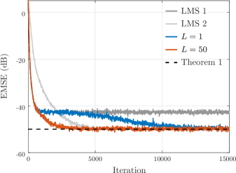
Figure 8: Steady-state analysis of a combination of LMS filters with coefficients feedback. Correlated stationary scenario (see Section VI): M=10𝑀10M=10, σu2=1superscriptsubscript𝜎𝑢21\sigma_{u}^{2}=1, σv2=103superscriptsubscript𝜎𝑣2superscript103\sigma_{v}^{2}=10^{-3}, γ=0.7𝛾0.7\gamma=0.7, μ1=0.01subscript𝜇10.01\mu_{1}=0.01, μ2=0.002subscript𝜇20.002\mu_{2}=0.002; Cyclic coefficients feedback: L=1𝐿1L=1, μ~=30~𝜇30\tilde{\mu}=30, β=0.9𝛽0.9\beta=0.9, and ϵ=102italic-ϵsuperscript102\epsilon=10^{-2} (normalized convex supervisor); L=50𝐿50L=50: μ~=10~𝜇10\tilde{\mu}=10, β=0.9𝛽0.9\beta=0.9, ϵ=103italic-ϵsuperscript103\epsilon=10^{-3}, (normalized convex supervisor).
Refer to caption
Figure 9: Tracking analysis of combinations with coefficients feedback. White nonstationary scenario (see Section VI): M=10𝑀10M=10, σu2=1superscriptsubscript𝜎𝑢21\sigma_{u}^{2}=1, σv2=102superscriptsubscript𝜎𝑣2superscript102\sigma_{v}^{2}=10^{-2}, μ1=0.08subscript𝜇10.08\mu_{1}=0.08, and μ2=0.005subscript𝜇20.005\mu_{2}=0.005; σq2=104superscriptsubscript𝜎𝑞2superscript104\sigma_{q}^{2}=10^{-4} until i=2000𝑖2000i=2000, then σq2105superscriptsubscript𝜎𝑞2superscript105\sigma_{q}^{2}\to 10^{-5} until i=4000𝑖4000i=4000, then σq2106superscriptsubscript𝜎𝑞2superscript106\sigma_{q}^{2}\to 10^{-6}. Parallel-independent (L𝐿L\to\infty): μ~=0.5~𝜇0.5\tilde{\mu}=0.5, β=0.9𝛽0.9\beta=0.9, and ϵ=102italic-ϵsuperscript102\epsilon=10^{-2} (normalized convex supervisor); Cyclic coefficients feedback: L=10𝐿10L=10, μ~=0.7~𝜇0.7\tilde{\mu}=0.7, β=0.7𝛽0.7\beta=0.7, and ϵ=102italic-ϵsuperscript102\epsilon=10^{-2} (normalized convex supervisor); VSS-LMS [4]: μ(i)=0.95μ(i1)+101e(i)2𝜇𝑖0.95𝜇𝑖1superscript101𝑒superscript𝑖2\mu(i)=0.95\cdot\mu(i-1)+10^{-1}\cdot e(i)^{2}, μmax=μ1subscript𝜇maxsubscript𝜇1\mu_{\text{max}}=\mu_{1}, and μmin=μ2subscript𝜇minsubscript𝜇2\mu_{\text{min}}=\mu_{2}.

VI Simulations

The numerical examples in this section illustrate both the performance of combinations with coefficients feedback and the theoretical results from the previous sections. They follow the data model introduced in Section IV, taking the regressor 𝒖isubscript𝒖𝑖\bm{u}_{i} to be a delay line that captures samples u(i)𝑢𝑖u(i) from a zero-mean Gaussian process with σu2=𝔼u(i)2superscriptsubscript𝜎𝑢2𝔼𝑢superscript𝑖2\sigma_{u}^{2}=\operatorname{\mathbb{E}}u(i)^{2}. For simulations with white input data, the u(i)𝑢𝑖u(i) are taken to be zero-mean Gaussian i.i.d. random variable. For simulations with correlated input data, the u(i)𝑢𝑖u(i) follow the first-order autoregressive model

u(i)=γu(i1)+1γ2x(i),𝑢𝑖𝛾𝑢𝑖11superscript𝛾2𝑥𝑖,u(i)=\gamma u(i-1)+\sqrt{1-\gamma^{2}}\,x(i)\text{,} (45)

where x(i)𝑥𝑖x(i) is a zero-mean Gaussian i.i.d. random variable with variance σu2superscriptsubscript𝜎𝑢2\sigma_{u}^{2} and 0<γ<10𝛾10<\gamma<1. Unless stated otherwise, all curves are ensemble averages of 300 independent realizations.
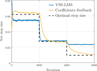
Refer to caption
Figure 10: Tracking analysis of combinations with coefficients feedback: equivalent step size. Same setting as Fig. 9.
Refer to caption
Figure 11: Transient analysis of a combination of LMS filters with coefficients feedback: convex supervisor. Correlated stationary scenario (see Section VI): M=10𝑀10M=10, σu2=1superscriptsubscript𝜎𝑢21\sigma_{u}^{2}=1, σv2=102superscriptsubscript𝜎𝑣2superscript102\sigma_{v}^{2}=10^{-2}, γ=0.7𝛾0.7\gamma=0.7, μ1=0.05subscript𝜇10.05\mu_{1}=0.05, μ2=0.005subscript𝜇20.005\mu_{2}=0.005, L=100𝐿100L=100, and μa=250subscript𝜇𝑎250\mu_{a}=250 (convex supervisor). Ensemble averages of 100010001000 realizations.
Refer to caption
Figure 12: Transient analysis of a combination of LMS filters with coefficients feedback: affine supervisor. White stationary scenario (see Section VI): M=7𝑀7M=7, σu2=1superscriptsubscript𝜎𝑢21\sigma_{u}^{2}=1, σv2=102superscriptsubscript𝜎𝑣2superscript102\sigma_{v}^{2}=10^{-2}, μ1=0.05subscript𝜇10.05\mu_{1}=0.05, μ2=0.01subscript𝜇20.01\mu_{2}=0.01, L=80𝐿80L=80, μη=2subscript𝜇𝜂2\mu_{\eta}=2, and η0.25𝜂0.25\eta\geq-0.25. Ensemble averages of 100010001000 realizations.

VI-A Steady-state and tracking performance

For a stationary system, i.e., for 𝒒i=0subscript𝒒𝑖0\bm{q}_{i}=0 in (12), Fig. 8 compares the steady-state results from Theorem (1) to numerical simulations using a convex supervisor. Given that the supervising parameter is constrained to [0,1]01[0,1], the performance models yield accurate predictions. As discussed in Section IV-A, if η𝜂\eta is unconstrained, coefficients feedback drives the net step size close to zero as in Fig. 7. Since Theorem 1 relies on the assumption that the supervisor has small variance, its estimate of η¯¯𝜂\bar{\eta} is no longer reliable. Nevertheless, (18) can still be used to estimate the steady-state EMSE for specific values of η¯¯𝜂\bar{\eta}. Moreover, the transient analysis from Theorem 2 can be used in this case (see Section VI-B).

To showcase the tracking capabilities of the coefficients feedback topology, let 𝒒isubscript𝒒𝑖\bm{q}_{i} in (12) be a zero-mean Gaussian random variable with covariance 𝑸=σq2𝑰𝑸superscriptsubscript𝜎𝑞2𝑰\bm{Q}=\sigma_{q}^{2}\bm{I}. Recall from Theorem 1 that for small L𝐿L its steady-state error is equivalent to that of a standalone LMS filter with step size μ¯¯𝜇\bar{\mu}, an affine/convex combination of the component filters step sizes. For illustration, we therefore compare its performance to the VSS-LMS filter from [4] in Fig. 9. The VSS-LMS parameters were designed to give good performance in the first, most stringent scenario (σq2=104superscriptsubscript𝜎𝑞2superscript104\sigma_{q}^{2}=10^{-4}). We also include the results for a parallel-independent combination.

Although the performance of both combinations and the VSS-LMS filter are comparable in the first scenario, the same does not hold as the nonstationarity level changes. In the two other scenarios (σq2=105superscriptsubscript𝜎𝑞2superscript105\sigma_{q}^{2}=10^{-5} and σq2=106superscriptsubscript𝜎𝑞2superscript106\sigma_{q}^{2}=10^{-6}), either the parallel-independent or the VSS-LMS has higher misadjustment. The parallel-independent topology performs well in the first and last scenarios because the step size of each component filter was chosen close to the optimal μosuperscript𝜇𝑜\mu^{o} in these cases (see Fig. 10). However, it performs worse when this is not the case. The VSS-LMS algorithm, although effective, is less robust than the normalized convex supervisor used by the combinations [28]. Thus, its performance is sensitive to the choice of parameters and it cannot track the optimal step size in the last scenario (Fig. 10).

VI-B Transient performance

Figs. 3b and 8 already showcased the effectiveness of coefficients feedback in addressing the convergence stagnation issue. Figs. 11 and 12 additionally illustrate the results from Theorem 2 for both convex and affine supervisors. Overall, the transient analysis matches the simulations. Small deviations occur in the convex supervisor case when the combination switches between component filters (see detail in Fig. 11a). This is due to the first-order approximation used to derive the supervisor variance recursion in Section V-C. This phenomenon is not as apparent in the affine supervisor simulations because (40)–(42) are exact when the activation function is linear (Fig. 12a). Still, the supervisor analyses show good agreement and display the same trends as the simulations (Figures 11b–c and 12b–c). Despite the cyclostationary behavior of the component filters due to coefficients feedback, notice that the mean supervising parameters converge to a constant steady-state regime. This observation was used to provide the asymptotic performance results from Theorem 1 without relying on a full transient analysis.

VII Conclusion

This paper proposed a new structure for the combination of adaptive filters by making use of cyclic coefficients feedback. This novel topology is able to theoretically describe standalone VSS adaptive algorithms as instances (L=1𝐿1L=1) of this combination. Steady-state, tracking, and transient analyses showed how cyclic coefficients feedback can improve performance of combinations by addressing the convergence stagnation issue, improving tracking misadjustment, and reducing the supervising parameter variance. Numerical simulations illustrated the good fit of the derived models and showed that existing parallel combinations can be effectively and efficiently improved using the techniques described in this work. This topology opens up new applications for combinations of AFs, such as complexity reduction [36] and rescue techniques [1].

Appendix A Proof of Proposition 1

Proof.

From the cyclic feedback relation (9), observe that L=1𝒘n,a=𝒘i1𝐿1subscript𝒘𝑛𝑎subscript𝒘𝑖1L=1\Rightarrow\bm{w}_{n,a}=\bm{w}_{i-1} for all i𝑖i. Thus, the update of the LMS component filters (1) becomes

𝒘n,i=𝒘i1+μn𝒖ie(i),n=1,2,formulae-sequencesubscript𝒘𝑛𝑖subscript𝒘𝑖1subscript𝜇𝑛subscript𝒖𝑖𝑒𝑖,𝑛12,\bm{w}_{n,i}=\bm{w}_{i-1}+\mu_{n}\bm{u}_{i}e(i)\text{,}\quad n=1,2\text{,} (46)

where we recall that e(i)=d(i)𝒖iT𝒘i1𝑒𝑖𝑑𝑖superscriptsubscript𝒖𝑖𝑇subscript𝒘𝑖1e(i)=d(i)-\bm{u}_{i}^{T}\bm{w}_{i-1} is the global output estimation error. The coefficients error vector statistics in (21) are obtained by first subtracting (46) from 𝒘iosubscriptsuperscript𝒘𝑜𝑖\bm{w}^{o}_{i} to get

𝒘~n,i=𝒘io𝒘i1μn𝒖ie(i),n=1,2.formulae-sequencesubscript~𝒘𝑛𝑖subscriptsuperscript𝒘𝑜𝑖subscript𝒘𝑖1subscript𝜇𝑛subscript𝒖𝑖𝑒𝑖,𝑛12.\widetilde{\bm{w}}_{n,i}=\bm{w}^{o}_{i}-\bm{w}_{i-1}-\mu_{n}\bm{u}_{i}e(i)\text{,}\quad n=1,2\text{.}

Then, notice that the random walk system model from (12) implies that 𝒘io𝒘i1=𝒘~i1+𝒒isubscriptsuperscript𝒘𝑜𝑖subscript𝒘𝑖1subscript~𝒘𝑖1subscript𝒒𝑖\bm{w}^{o}_{i}-\bm{w}_{i-1}=\widetilde{\bm{w}}_{i-1}+\bm{q}_{i}. Hence, we can write

𝒘~n,i=𝒘~i1+𝒒iμn𝒖ie(i),n=1,2.formulae-sequencesubscript~𝒘𝑛𝑖subscript~𝒘𝑖1subscript𝒒𝑖subscript𝜇𝑛subscript𝒖𝑖𝑒𝑖,𝑛12.\widetilde{\bm{w}}_{n,i}=\widetilde{\bm{w}}_{i-1}+\bm{q}_{i}-\mu_{n}\bm{u}_{i}e(i)\text{,}\quad n=1,2\text{.} (47)

Taking the expectation of the appropriate inner products of (47) results in

𝔼𝒘~n,i2𝔼superscriptnormsubscript~𝒘𝑛𝑖2\displaystyle\operatorname{\mathbb{E}}\left\|\widetilde{\bm{w}}_{n,i}\right\|^{2} =𝔼𝒘~i12+Tr(𝑸)absent𝔼superscriptnormsubscript~𝒘𝑖12Tr𝑸\displaystyle=\operatorname{\mathbb{E}}\left\|\widetilde{\bm{w}}_{i-1}\right\|^{2}+\operatorname{Tr}(\bm{Q})
2μn𝔼ea(i)e(i)+μn2𝔼𝒖i2e(i)22subscript𝜇𝑛𝔼subscript𝑒𝑎𝑖𝑒𝑖superscriptsubscript𝜇𝑛2𝔼superscriptnormsubscript𝒖𝑖2𝑒superscript𝑖2\displaystyle-2\mu_{n}\operatorname{\mathbb{E}}e_{a}(i)e(i)+\mu_{n}^{2}\operatorname{\mathbb{E}}\left\|\bm{u}_{i}\right\|^{2}e(i)^{2} (48a)
𝔼𝒘~1,iT𝒘~2,i𝔼superscriptsubscript~𝒘1𝑖𝑇subscript~𝒘2𝑖\displaystyle\operatorname{\mathbb{E}}\widetilde{\bm{w}}_{1,i}^{T}\widetilde{\bm{w}}_{2,i} =𝔼𝒘~i12+Tr(𝑸)absent𝔼superscriptnormsubscript~𝒘𝑖12Tr𝑸\displaystyle=\operatorname{\mathbb{E}}\left\|\widetilde{\bm{w}}_{i-1}\right\|^{2}+\operatorname{Tr}(\bm{Q})
(μ1+μ2)𝔼ea(i)e(i)subscript𝜇1subscript𝜇2𝔼subscript𝑒𝑎𝑖𝑒𝑖\displaystyle-(\mu_{1}+\mu_{2})\operatorname{\mathbb{E}}e_{a}(i)e(i) (48b)
+μ1μ2𝔼𝒖i2e(i)2.subscript𝜇1subscript𝜇2𝔼superscriptnormsubscript𝒖𝑖2𝑒superscript𝑖2.\displaystyle+\mu_{1}\mu_{2}\operatorname{\mathbb{E}}\left\|\bm{u}_{i}\right\|^{2}e(i)^{2}\text{.}

where we used the fact that 𝔼𝒒i2=Tr(𝑸)𝔼superscriptnormsubscript𝒒𝑖2Tr𝑸\operatorname{\mathbb{E}}\left\|\bm{q}_{i}\right\|^{2}=\operatorname{Tr}(\bm{Q}) and that all terms linear in 𝒒isubscript𝒒𝑖\bm{q}_{i} vanish due to A.2.

Note that under A.5, it holds that 𝔼𝒖i2e(i)2=Tr(𝑹u)𝔼e(i)2𝔼superscriptnormsubscript𝒖𝑖2𝑒superscript𝑖2Trsubscript𝑹𝑢𝔼𝑒superscript𝑖2\operatorname{\mathbb{E}}\left\|\bm{u}_{i}\right\|^{2}e(i)^{2}=\operatorname{Tr}(\bm{R}_{u})\operatorname{\mathbb{E}}e(i)^{2} and that A.1 implies that 𝔼e(i)2=ζ(i)+σv2𝔼𝑒superscript𝑖2𝜁𝑖superscriptsubscript𝜎𝑣2\operatorname{\mathbb{E}}e(i)^{2}=\zeta(i)+\sigma_{v}^{2} and 𝔼ea(i)e(i)=ζ(i)𝔼subscript𝑒𝑎𝑖𝑒𝑖𝜁𝑖\operatorname{\mathbb{E}}e_{a}(i)e(i)=\zeta(i). Using these relations, (48) can written as (21). ∎

Appendix B Proof of Proposition 2

Proof.

We start by evaluating the global EMSE minimizer ηosuperscript𝜂𝑜\eta^{o}. Fix η𝜂\eta in the a priori error relation (15) to obtain

ζ(i)=𝔼[ηe1,a(i)+(1η)e2,a(i)]2\zeta(i)=\operatorname{\mathbb{E}}\left[\eta e_{1,a}(i)+(1-\eta)e_{2,a}(i)\right]^{2} (49)

by recalling that ζ(i)=𝔼ea(i)2𝜁𝑖𝔼subscript𝑒𝑎superscript𝑖2\zeta(i)=\operatorname{\mathbb{E}}e_{a}(i)^{2}. Since η𝜂\eta is fixed, we can expand (49) to get, as i𝑖i\to\infty,

ζ=η2ζ1+2η(1η)ζ12+(1η)2ζ2.𝜁superscript𝜂2subscript𝜁12𝜂1𝜂subscript𝜁12superscript1𝜂2subscript𝜁2.\zeta=\eta^{2}\zeta_{1}+2\eta(1-\eta)\zeta_{12}+(1-\eta)^{2}\zeta_{2}\text{.} (50)

We can find ηosuperscript𝜂𝑜\eta^{o} by setting the derivative of (50) to zero. Explicitly,

ζη=0ηΔζ1(1η)Δζ2(i)=0,𝜁𝜂0𝜂Δsubscript𝜁11𝜂Δsubscript𝜁2𝑖0,\frac{\partial\zeta}{\partial\eta}=0\Leftrightarrow\eta\Delta\zeta_{1}-(1-\eta)\Delta\zeta_{2}(i)=0\text{,}

where Δζn=ζ1ζ12Δsubscript𝜁𝑛subscript𝜁1subscript𝜁12\Delta\zeta_{n}=\zeta_{1}-\zeta_{12}. Hence,

ηo=Δζ2Δζ1+Δζ2.superscript𝜂𝑜Δsubscript𝜁2Δsubscript𝜁1Δsubscript𝜁2.\eta^{o}=\frac{\Delta\zeta_{2}}{\Delta\zeta_{1}+\Delta\zeta_{2}}\text{.} (51)

To show that (51) is also a fixed point of the mean supervisor update, take the expected value of (6a) under the supervisor separation assumption A.4 to get

a¯(i)=a¯(i1)+μa𝔼e(i)[y1(i)y2(i)]𝔼f[a(i1)],¯𝑎𝑖¯𝑎𝑖1subscript𝜇𝑎𝔼𝑒𝑖delimited-[]subscript𝑦1𝑖subscript𝑦2𝑖𝔼superscript𝑓delimited-[]𝑎𝑖1,\bar{a}(i)=\bar{a}(i-1)+\mu_{a}\operatorname{\mathbb{E}}e(i)\left[y_{1}(i)-y_{2}(i)\right]\operatorname{\mathbb{E}}f^{\prime}[a(i-1)]\text{,} (52)

where a¯(i)=𝔼a(i)¯𝑎𝑖𝔼𝑎𝑖\bar{a}(i)=\operatorname{\mathbb{E}}a(i). Any fixed point of (52) is such that

μa𝔼e(i)[y1(i)y2(i)]𝔼f[a(i1)]=0subscript𝜇𝑎𝔼𝑒𝑖delimited-[]subscript𝑦1𝑖subscript𝑦2𝑖𝔼superscript𝑓delimited-[]𝑎𝑖10\mu_{a}\operatorname{\mathbb{E}}e(i)\left[y_{1}(i)-y_{2}(i)\right]\operatorname{\mathbb{E}}f^{\prime}[a(i-1)]=0

and since μasubscript𝜇𝑎\mu_{a} and fsuperscript𝑓f^{\prime} are strictly positive, this condition reduces to

𝔼e(i)[y1(i)y2(i)]=0.𝔼𝑒𝑖delimited-[]subscript𝑦1𝑖subscript𝑦2𝑖0.\operatorname{\mathbb{E}}e(i)\left[y_{1}(i)-y_{2}(i)\right]=0\text{.} (53)

From (53), we obtain an expression for ηsuperscript𝜂\eta^{\star} by expanding the estimation error and the component filters outputs. Explicitly, fixing ηsuperscript𝜂\eta^{\star} in (15)–(16), we can then rewrite (53) as

𝔼[ηea,1(i)+(1η)ea,2(i)+v(i)]×[ea,2(i)ea,1(i)]=0.𝔼superscript𝜂subscript𝑒𝑎1𝑖1superscript𝜂subscript𝑒𝑎2𝑖𝑣𝑖delimited-[]subscript𝑒𝑎2𝑖subscript𝑒𝑎1𝑖0.\operatorname{\mathbb{E}}\left[\eta^{\star}\,e_{a,1}(i)+\left(1-\eta^{\star}\right)e_{a,2}(i)+v(i)\right]\times{}\\ \left[e_{a,2}(i)-e_{a,1}(i)\right]=0\text{.} (54)

From the data model assumption A.1, all terms linear in v(i)𝑣𝑖v(i) vanish, so that as i𝑖i\to\infty, (54) becomes

(1η)ζ2+(2η1)ζ12ηζ1=0,1superscript𝜂subscript𝜁22superscript𝜂1subscript𝜁12superscript𝜂subscript𝜁10,(1-\eta^{\star})\zeta_{2}+(2\eta^{\star}-1)\zeta_{12}-\eta^{\star}\zeta_{1}=0\text{,}

which can be rearranged as in (51). ∎

Acknowledgment

The authors would like to thank Dr. Wilder Bezerra Lopes, Prof. Vítor Heloiz Nascimento, and Prof. Magno T. M. Silva for fruitful discussions on this topic.

References

  • [1] A. Sayed, Adaptive filters.   Wiley-IEEE Press, 2008.
  • [2] P. Diniz, Adaptive filtering: Algorithms and practical implementation, 4th ed.   Springer, 2013.
  • [3] R. Harris, D. Chabries, and F. Bishop, “Variable step (VS) adaptive filter algorithm,” IEEE Trans. Signal Process., vol. 34, pp. 309–316, 1986.
  • [4] R. Kwong and E. Johnston, “A variable step size LMS algorithm,” IEEE Trans. Signal Process., vol. 40[7], pp. 1633–1642, 1992.
  • [5] V. Mathews and Z. Xie, “A stochastic gradient adaptive filter with gradient adaptive step size,” IEEE Trans. Signal Process., vol. 41[6], pp. 2075–2087, 1993.
  • [6] K. Mayyas and T. Aboulnasr, “A robust variable step size LMS-type algorithm: Analysis and simulations,” in ICASSP, 1995, pp. 1408–1411.
  • [7] H.-C. Shin, A. Sayed, and W.-J. Song, “Variable step-size NLMS and affine projection algorithms,” IEEE Signal Process. Lett., vol. 11, pp. 132–135, 2004.
  • [8] A. Singer and M. Feder, “Universal linear prediction by model order weighting,” IEEE Trans. Signal Process., vol. 47[10], pp. 2685–2699, 1999.
  • [9] S. Kozat and A. Singer, “Further results in multistage adaptive filtering,” in ICASSP, 2002, pp. 1329–1332.
  • [10] J. Arenas-García, A. Figueiras-Vidal, and A. Sayed, “Mean-square performance of a convex combination of two adaptive filters,” IEEE Trans. Signal Process., vol. 54[3], pp. 1078–1090, 2006.
  • [11] Y. Zhang and J. Chambers, “Convex combination of adaptive filters for a variable tap-length LMS algorithm,” IEEE Signal Process. Lett., vol. 13[10], pp. 628–631, 2006.
  • [12] N. Bershad, J. Bermudez, and J.-Y. Tourneret, “An affine combination of two LMS adaptive filters—transient mean-square analysis,” IEEE Trans. Signal Process., vol. 56[5], pp. 1853––1864, 2008.
  • [13] M. Silva and V. Nascimento, “Improving the tracking capability of adaptive filters via convex combination,” IEEE Trans. Signal Process., vol. 56[7], pp. 3137––3149, 2008.
  • [14] C. Lopes, E. Satorius, P. Estabrook, and A. Sayed, “Efficient adaptive carrier tracking for Mars to Earth communications during entry, descent and landing,” in SSP, 2007, pp. 517–521.
  • [15] J. Arenas-García and A. Figueiras-Vidal, “Adaptive combination of IPNLMS filters for robust sparse echo cancellation,” in MLSP, 2008, pp. 221–226.
  • [16] C. Lopes, E. Satorius, P. Estabrook, and A. Sayed, “Adaptive carrier tracking for Mars to Earth communications during entry, descent, and landing,” IEEE Trans. Aerosp. Electron. Syst., vol. 46[4], pp. 1865–1879, 2010.
  • [17] L. Azpicueta-Ruiz, M. Zeller, A. Figueiras-Vidal, J. Arenas-García, and W. Kellermann, “Adaptive combination of Volterra kernels and its application to nonlinear acoustic echo cancellation,” IEEE Trans. Audio, Speech, Signal Process., vol. 19[1], pp. 97–110, 2011.
  • [18] W. Lopes and C. Lopes, “Incremental-cooperative strategies in combination of adaptive filters,” in ICASSP, 2011, pp. 4132–4135.
  • [19] L. Chamon, W. Lopes, and C. Lopes, “Combination of adaptive filters with coefficients feedback,” in ICASSP, 2012, pp. 3785–3788.
  • [20] L. Chamon, H. Ferro, and C. Lopes, “A data reusage algorithm based on incremental combination of LMS filters,” in Asilomar Conference on Signals, Systems and Computers, 2012.
  • [21] V. Nascimento and R. de Lamare, “A low-complexity strategy for speeding up the convergence of convex combinations of adaptive filters,” in ICASSP, 2012, pp. 3553–3556.
  • [22] H. Ferro, L. Chamon, and C. Lopes, “FIR-IIR adaptive filters hybrid combination,” IET Electronics Letters, vol. 50[7], pp. 501–503, 2014.
  • [23] L. Azpicueta-Ruiz, A. Figueiras-Vidal, and J. Arenas-García, “A normalized adaptation scheme for the convex combination of two adaptive filters,” in ICASSP, 2008, pp. 3301–3304.
  • [24] R. Candido, M. Silva, and V. Nascimento, “Transient and steady-state analysis of the affine combination of two adaptive filters,” IEEE Trans. Signal Process., vol. 58[8], pp. 4064–4078, 2010.
  • [25] V. Nascimento, M. Silva, R. Candido, and J. Arenas-García, “A transient analysis for the convex combination of adaptive filters,” in SSP, 2009, pp. 53–56.
  • [26] S. Kozat, A. Singer, A. Erdogan, and A. Sayed, “Unbiased model combinations for adaptive filtering,” IEEE Trans. Signal Process., vol. 58[8], pp. 4421–4427, 2010.
  • [27] S. Kozat, A. Erdogan, A. Singer, and A. Sayed, “Transient analysis of adaptive affine combinations,” IEEE Trans. Signal Process., vol. 59[12], pp. 6227–6232, 2011.
  • [28] J. Arenas-García, L. Azpicueta-Ruiz, M. Silva, V. Nascimento, and A. Sayed, “Combinations of adaptive filters: Performance and convergence properties,” IEEE Signal Process. Mag., vol. 33[1], pp. 120–140, 2016.
  • [29] M. Lazaro-Gredilla, L. Azpicueta-Ruiz, A. Figueiras-Vidal, and J. Arenas-García, “Adaptively biasing the weights of adaptive filters,” IEEE Trans. Signal Process., vol. 58[7], pp. 3890–3895, 2010.
  • [30] V. Nascimento, M. Silva, L. Azpicueta-Ruiz, and J. Arenas-Garcia, “On the tracking performance of combinations of least mean squares and recursive least squares adaptive filters,” in IEEE International Conference on Acoustics Speech and Signal Processing, 2010, pp. 3710–3713.
  • [31] Y. Huang, J. Benesty, and J. Chen, Acoustic MIMO Signal Processing.   Springer, 2006.
  • [32] H. So and P. Ching, “Comparative study of five LMS-based adaptive time delay estimators,” IEE Proc. Radar, Sonar and Nav., vol. 148[1], pp. 9–15, 2001.
  • [33] B. Widrow and E. Walach, Adaptive inverse control: a signal processing approach.   Wiley-IEEE Press, 2008.
  • [34] R. Candido, M. Silva, and V. Nascimento, “Affine combinations of adaptive filters,” in Asilomar Conference on Signals, Syst. and Comput., 2008, pp. 236–240.
  • [35] M. Silva, V. Nascimento, and J. Arenas-García, “A transient analysis for the convex combination of two adaptive filters with transfer of coefficients,” in ICASSP, 2010, pp. 3842––3845.
  • [36] L. Chamon and C. Lopes, “There’s plenty of room at the bottom: Incremental combinations of sign-error LMS filters,” in International Conference in Acoustic, Speech, and Signal Processing (ICASSP), 2014.