Noetherian symmetries of noncentral forces with drag term

Abstract

We consider the Noetherian symmetries of second-order ODEs subjected to forces with nonzero curl. Both position and velocity dependent forces are considered. In the former case the first integrals are shown to follow from the symmetries of the celebrated Emden-Fowler equation.

Dedicated to Sir Michael Berry on his 75th birthday with great respect and admiration

Mathematics Classification (2010)

: 34C14, 34C20.

Keywords:

Curl forces, anisotropic central forces, Emden-Fowler equation,

1 Introduction

The motion of a particle under the influence of a central force is a standard topic of Classical Mechanics and is treated extensively in almost all text books on the subject. The radial nature of the force implies the conservation of angular momentum and greatly simplifies the analysis of the radial equation, with the orbit being determined by Binet’s formula. However, in most cases the possibility of the central forces being of anisotropic character is usually not treated.
Newtonian forces depending on position and having a nonvanishing curl are usually termed as curl forces. In [3]it was shown that for a plananr isotropic force, $F=f(r){\mathbf{e}}_{\theta}$ when $f(r)=r^{\mu}$, with a nonvanishing curl one can quite generally map the radial equation to the Emden-Fowler equation by defining a transformation of both the independent and dependent variables.

Incidentally the issue of such forces did not escape Whittaker’s [21] attention. In his book the problem of the most general field of force under which a given curve can be described is treated. Starting with a curve $\phi(x,y)=c$ the general form of the component of the acceleration $(X,Y)$ are derived. This expression involves an arbitrary function $u$ of $x,y$, which is related to the square of the velocity of particle. In general the curl condition is $\partial_{x}Y-\partial_{y}X\neq 0$. Of course there is no mention of the possibility of deriving Hamiltonians in this context. In recent times a fairly general treatment of the Ermakov [2] and generalised Ermakov system [13] was also performed which treatment involved forces depending upon both $r$ and $\theta$ with a nonvanishing curl. These analyses were motivated mainly by a desire to examine if the equation was linearisable. Berry and Shukla [4] showed that the force on a particle with complex electric polarizability is known to be not derivable from a potential, i.e., its curl is nonzero. In general curl forces are Newtonian but not Hamiltonian or Lagrangian. However, recently the Hamiltonian formalism of curl forces has been studied in [5].

In [3] the authors performed a detailed analysis of the nature of the motion for specific values of the exponent $\mu$ of the force. In particular their analysis of the case $\mu=-1$ is interesting and begs the question of the possible implications of such a motion evoking as it does an uncanny similarity with the Aharonov-Bohm effect. Furthermore in course of their analysis they determined two first integrals of motion corresponding to $\mu=-3/2$ and $\mu=-5/3$, respectively. The Emden-Fowler (EF) equation which forms the cornerstone of their work is a well-known nonlinear ordinary differential equation and has been extensively studied by Leach et al [15, 16, 17] from the point of view of its symmetries. Consequently one of the objectives of the present article is to show that these first integrals are actually the fruits of the existence of a variational (Noetherian) symmetry of the Emden-Fowler equation.

Consider a Lagrangian system $L:{\mathbb{R}}\times TQ\to{\mathbb{R}}$, on a configuration space $Q$ with local coordinates $q=(q_{1},\cdots,q_{n})$. The action of an one-parameter group of diffeomorphisms $\Phi_{s}$ on ${\mathbb{R}}\times Q$ with the induced vector field reads

$${\cal X}=\eta(t,q)\frac{\partial}{\partial t}+\sum_{i}(\xi^{i}(t,q)\frac{\partial}{\partial q_{i}}+\hat{\xi}^{i}(t,q)\frac{\partial}{\partial{\dot{q}}_{i}}),$$

where

$$\hat{\xi}^{i}(t,q)=\frac{\partial\xi^{i}}{\partial t}-{\dot{q}}_{i}\frac{\partial\eta}{\partial t}+\sum_{j}(\frac{\partial\xi^{i}}{\partial q_{j}}{\dot{q}}_{j}-{\dot{q}}_{i}\frac{\partial\eta}{\partial\partial q_{j}}{\dot{q}}_{j}).$$

The group $\Phi_{s}$ is a Noetherian symmetry of the Lagrangian system if it preserves the action functional $S=\int_{a}^{b}L(t,q,\dot{q})dt$, if

$$\frac{\partial L}{\partial t}\eta+\sum_{i}(\xi^{i}(t,q)\frac{\partial L}{\partial q_{i}}+\hat{\xi}^{i}(t,q)\frac{\partial L}{\partial{\dot{q}}_{i}})+L(\frac{\partial\eta}{\partial t}+\frac{\partial\eta}{\partial q_{j}}{\dot{q}}_{j})=0$$ (1.1)

The Noether theorem states that if $\Phi_{s}$ is a Noether symmetry then

$${\mathbb{J}}(t,q,{\dot{q}})=\sum_{i}\frac{\partial L}{\partial{\dot{q}}_{i}}(\xi^{i}-\eta{\dot{q}}_{i})+L\eta.$$ (1.2)

There are several possible ways to generalise the Berry-Shukla construction. In this paper we briefly outline the curl force in the presence of a coordinate-dependent dissipative force and show that the system can be mapped to the Lane-Emden equation, which appears in the study of stellar structure. Polytropes are a family of equations of state for which the pressure $P$ is given as a power of density $\rho$, $P=\kappa\rho^{\gamma}$, where $\kappa$ and $\gamma$ are constants. The Lane-Emden equation

$$\frac{1}{\xi^{2}}\frac{d}{d\xi}\left(\xi^{2}\frac{d\theta}{d\xi}\right)+\theta^{n}=0$$

combines this $P$ and $\rho$ relation and the equation of hydrostatic equilibrium. This was originally proposed by Jonathan Lane [14] and was analysed by Emden [8]. The Lane-Emden equation can be solved analytically only for a few special, integer values of the index $n:0,1$ and $5$ [18] and for all other values of $n$ we must resort to numerical solutions. Several applications of the Emden-Fowler and Lane-Emden equations of various forms arising in astrophysics [7] and nonlinear dynamics have been reported. The reader is also referred to the now oldish paper by Wang [20] for a sampling of citations of papers dealing with the equation using various approaches.

The paper is organized as follows. In Section 2 we introduce nonisotropic curl forces and briefly recollect the results of Athorne [2] and Haas and Goedert [13]. In Section 3 we show that from the particular solution of the EF equation it is possible to arrive at the results of [3]. Finally by introducing the Lagrangian of the Emden-Fowler equation and taking into consideration its symmetries one can easily derive the first integrals stated in Berry’s and Shukla’s paper.

2 Motion under noncentral forces

The motion of a point particle in the plane, taken for convenience to be of unit mass, is best studied in terms of polar coordinates, $r$ and $\theta$, in terms of which the components of the equation of motion are

$$\ddot{r}-r\dot{\theta}^{2} =F_{r}(r,\theta),$$ (2.1)

$$r\ddot{\theta}+2\dot{r}\dot{\theta} =F_{\theta}(r,\theta).$$ (2.2)

In plane polar coordinates the condition $\nabla\times F\neq 0$ translates into the requirement that

$$\frac{\partial}{\partial r}\left(rF_{\theta}\right)\neq\frac{\partial F_{r}}{\partial\theta}.$$ (2.3)

For the generalised Ermakov system of [13] the radial and transverse components of the force are given by

$$F_{r}(r,\theta) =-w^{2}r+\frac{1}{r^{3}}U(\theta),$$ (2.4)

$$F_{\theta}(r,\theta) =-\frac{1}{r^{3}}\frac{dV}{d\theta}.$$ (2.5)

Here $U(\theta)$ and $V(\theta)$ are arbitrary functions and one may verify that the force satisfies (2.3) and is therefore a curl force. For the generalised Ermakov system there exists the well-known Lewis-Ray-Reid (LRR) invariant

$$I=\frac{1}{2}(r^{2}\dot{\theta})^{2}+V(\theta).$$ (2.6)

In this connection mention has to be made of the method used by Gorringe and Leach [10] to deduce a first integral for a planar system governed by a noncentral force the radial and tangential components of which are given by

$$F_{r}(r,\theta)=-\left[\frac{U^{\prime\prime}(\theta)+U(\theta)}{r^{2}}+\frac{2V^{\prime}(\theta)}{r^{3/2}}\right],\;\;F_{\theta}(r,\theta)=-\frac{V(\theta)}{r^{3/2}}.$$

Here $U(\theta)$ and $V(\theta)$ are arbitrary functions. Note that for such a force $\nabla\times F\neq 0$ if and only if $U(\theta)$ and $V(\theta)$ are not sinusoidal functions of their arguments.

In [2] a class of dynamical systems was considered which included the autonomous Ermakov system and the anisotropic Keplerian central force systems and it was shown that they were linearisable up to a pair of quadratures. In both [13] and [2] the possibility of linearisation rested upon the existence of the LRR invariant which was exploited for this purpose. The central feature of the demonstration consisted in the transformation of the radial coordinate $r$ by invoking an inverse transformation of the form $\psi=\rho(t)/r$ and in using the LRR invariant to replace the time derivative with the derivative with respect to the angular coordinate, $\theta$, via the relation $\dot{\theta}=h(\theta;I)/r^{2}$ obtained from (2.6) with $h^{2}=2(I-V(\theta))$. For the generalised Ermakov system Hass and Goedert then showed that the resulting form of the radial equation is

$$h^{2}\frac{d^{2}\psi}{d\theta^{2}}+\frac{1}{2}\frac{\partial h^{2}}{\partial\theta}\frac{d\psi}{d\theta}+(h^{2}+f(\theta))\psi=\frac{\rho^{3}(\ddot{\rho}+w^{2}\rho)}{\psi^{3}}.$$ (2.7)

Finally to achieve linearisation they demanded that the right-hand-side be of the form

$$\frac{\rho^{3}(\ddot{\rho}+w^{2}\rho)}{\psi^{3}}=a(\theta;I)\frac{d\psi}{d\theta}+b(\theta;I)\psi+c(\theta;I),$$ (2.8)

where $a$, $b$ and $c$ are arbitrary functions of their respective arguments. This condition imposes the necessary restrictions upon the frequency $w$. If one sets $\ddot{\rho}+w^{2}\rho=0$, then of course (2.7) automatically becomes linear. To illustrate the above procedure we consider an example.

$$\ddot{r}-r\dot{\theta}^{2}=0,$$ (2.9)

$$r\ddot{\theta}+2\dot{r}\dot{\theta}=\frac{1}{r^{3}}\sin\theta.$$ (2.10)

The force $F=\sin\theta/r^{3}{\mathbf{e}}_{\theta}$ is single-valued and periodic in the angular coordinate and is in the transverse direction. It is clear that $\nabla\times F=-2\sin\theta/r^{4}$ and is nonvanishing provided $\theta\neq\pm\pi$. Comparison with (2.4) shows that $U(\theta)=0$ and $V(\theta)=\cos\theta$ and the LRR invariant yields $\dot{\theta}=h^{2}(\theta;I)/r^{2}$, where $h^{2}=2(I-\cos\theta)$. Under the transformation $r=1/\psi$ we find that (2.7) reduces to

$$\frac{d^{2}\psi}{d\theta^{2}}+\frac{\sin\theta}{(I-\cos\theta)}\frac{d\psi}{d\theta}+\psi=0.$$ (2.11)

Some numerical solutions of the latter equation and for $|I|>1$ are given in figures 1 and 2. It is now straightforward to deduce the basis of solutions. While for $|I|<1$ in 3.

Remark: The LRR invariant is marked by an absence of any dependence upon the radial velocity and the procedure described above relies upon this as it enables one to solve for $\dot{\theta}$ in terms of $(r,\theta)$ only.

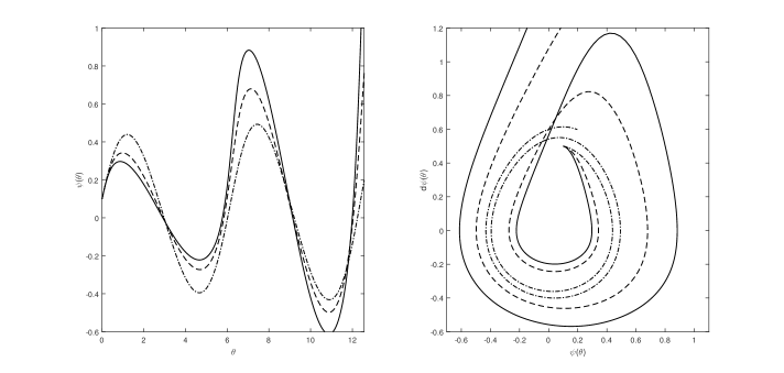
Figure 1: Numerical solution of equation 2.11) for different values of the constant of motion I greater than one. Solid line is for $I=1.1$, dash-dash line is for $I=1.2$, while dash-dot line is for $I=2$. Left figure is the $\theta-\psi$ diagram while right figure is the phase portrait $\psi-d\psi$

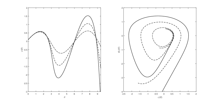
Figure 2: Numerical solution of equation (2.11) for different values of the constant of motion I, smaller than minus one. Solid line is for $I=1.1$, dash-dash line is for $I=-1.2$, while dash-dot line is for $I=-2$. Left figure is the $\theta-\psi$ diagram while right figure is the phase portrait $\psi-d\psi$

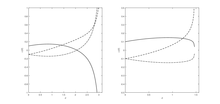
Figure 3: Numerical solution of equation (2.11) for $I=-1$ (left figure) awnd $I=0.5$ (right figure). Solid line is for the initial conditions $(0.1,0.1)$, dash-dash line is for $(-0.1,0.1)$ while dash-dot line is for the initial condition $(0.1,-0.1)$

A depiction of the orbit of the motion in the plane, $(r,\,\theta)$, for the system described by equations (2.9) and (2.10) may be obtained by the numerical evaluation of

$$rr^{\prime\prime}-2r^{\prime 2}+\frac{rr^{\prime}\sin\theta}{2(I-\cos\theta)}-r^{2}=0$$ (2.12)

in which the prime denotes differentiation with respect to the polar angle, $\theta$, or by that of (2.11). In both cases it is necessary to substitute the value of the Lewis-Ray-Reid Invariant. We provide two orbits, one for each option, which suggest that the latter is preferable even if geometrically less satisfactory.

3 Isotropic noncentral forces

Following Berry and Shukla we assume

$$\ddot{r}-r\dot{\theta}^{2}=0,$$ (3.1)

$$r\ddot{\theta}+2\dot{r}\dot{\theta}=f(r).$$ (3.2)

In general it is assumed that $f(r)=Cr^{\mu}$, where $C$ is a constant and may be scaled to unity. Clearly $F=f(r){\mathbf{e}}_{\theta}$ and the condition $\nabla\times F\neq 0$ implies that $\partial(rf(r))/\partial r\neq 0$ which precludes the case $f(r)=C/r$, i.e., the $\mu=-1$ case which was separately examined in detail in their work. In order to map the system (3.1)-(3.2) to the Emden-Fowler equation they introduced the transformation $(r,\theta)\longrightarrow(\tilde{T},\tilde{J})$, where $\tilde{J}=r^{2}\dot{\theta}$ is the angular momentum and is not an invariant and $\tilde{T}$ is the integrated torque defined by

$$\tilde{T}=\int rf(r)dr.$$ (3.3)

It follows from (3.2) that

$$\frac{d\tilde{J}}{dt}=rf(r)$$

and therefore

$$\tilde{T}^{\prime}(\tilde{J})=\dot{r}.$$ (3.4)

Consequently, differentiating with respect to $t$ and using (3.1) and (3.2), we obtain

$$\tilde{T}^{\prime\prime}(\tilde{J})=\frac{\tilde{J}^{2}}{r^{4}f(r)}.$$ (3.5)

Thus, when $f(r)=r^{\mu}$, we have, on making use of (3.3) in (3.5),

$$\tilde{T}^{\prime\prime}(\tilde{J})=A\tilde{J}^{n}\tilde{T}^{m},$$ (3.6)

where

$$A=(\mu+2)^{m},\;\;\;m=-\frac{\mu+4}{\mu+2},\;\;\;n=2.$$ (3.7)

Eqn. (3.6) is the well-known Emden-Fowler equation [15, 16, 17, 11]. The scaling transformations,

$$J=(\mu+2)^{1/n+2}\tilde{J}\quad\mbox{\rm and}\quad T=(\mu+2)\tilde{T},$$ (3.8)

enable us to remove the factor $A$ in the Emden-Fowler equation which now has the appearance

$$T^{\prime\prime}(J)=J^{n}T^{m}\;\;\mbox{with}\;\;n=2,m=-\frac{\mu+4}{\mu+2}.$$ (3.9)

Extending the technique of integrable modulation we obtain [12] the following proposition.

Proposition 3.1

The second-order ordinary differential equation    $T^{{\prime}{\prime}}+dJ^{n}T^{m}=0$ admits a first integral of the form

$$I=\frac{1}{2}(T^{\prime}J-T)^{2}+V(J,T)$$

where $V(J,T)=dJ^{n+2}T^{m+1}/(m+1)$ and $n+m=-3$.

Hence in our case $n=2$ implies $m=-5$.

Now it is known that (3.9) admits the particular solution

$$T(J)=\Lambda J^{(n+2)/(1-m)},\;\;m\neq 1,$$ (3.10)

where

$$\Lambda=\left[\frac{(n+2)(n+m+1)}{(m-1)^{2}}\right]^{1/m-1}.$$ (3.11)

Note that $m=1$ corresponds to $\mu=-3$ and it follows therefore that this case must be separately analysed. In fact it causes (3.9) to reduce to the linear equation

$$T^{\prime\prime}(J)=J^{2}T(J)$$

and may also be analysed by the methods of Section 2 since it corresponds to setting $V(\theta)=-\theta$ in(3.1) and (3.2) which admits the first integral

$$I=\frac{1}{2}(r^{2}\dot{\theta})^{2}-\theta$$ (3.12)

and leads to the linear equation

$$\frac{d^{2}\psi}{d\theta^{2}}+\frac{1}{(\theta+I)}\frac{d\psi}{d\theta}+\psi=0.$$ (3.13)

Consequently on the level surface, $I=c$, if we set $x=\theta+c$ then the above equation becomes

$$\frac{d^{2}\psi}{dx^{2}}+\frac{1}{x}\frac{d\psi}{dx}+\psi=0.$$

Moreover from (3.11) we observe that, as $n=2$, so, when $m=-3$, then $\Lambda=0$ and the solution is trivial. However, $m=-3$ corresponds to $\mu=-1$ and the force $f(r)=1/r$ therefore requires special treatment.

From (3.3) after taking into account the scaling we have

$$T=[r^{\mu+2}-r_{0}^{\mu+2}],$$ (3.14)

where $r_{0}$ is the initial position, which gives $T$ as a function of $r$ while (3.10) gives $T$ as a function of $J$, the angular momentum. By combining these we obtain $J$ as a function of $r$ given by

$$J=\left[\frac{1}{\Lambda}(r^{\mu+2}-r_{0}^{\mu+2})\right]^{\frac{1-m}{n+2}}.$$ (3.15)

The equation for the orbit can be obtained using the fact the (3.4) gives

$$\dot{r}=\frac{dr}{d\theta}\dot{\theta}=T^{\prime}(J)$$

so that

$$\frac{d\theta}{dr}=\frac{J}{r^{2}T^{\prime}(J)},$$ (3.16)

whence using (3.10) and (3.15) we obtain the final equation determining the orbit as

$$\frac{d\theta}{dr}=\left(\frac{1-m}{n+2}\right)\Lambda^{-\frac{2(1-m)}{n+2}}(r^{\mu+2}-r_{0}^{\mu+2})^{-\frac{2(n+m+3)}{n+2}}.$$ (3.17)

The solutions of $r$ and $\theta$ as functions of $t$ follow from (3.2) which upon taking into consideration the scaling of $\tilde{J}$ becomes

$$(\mu+2)^{-1/n+2}\frac{dJ}{dt}=rf(r).$$

Scaling of the time, $t\longrightarrow\tau=(\mu+2)^{1/n+2}t$, causes it to become $dJ/d\tau=rf(r)$ so that

$$\tau=\int\frac{dJ}{dr}\frac{dr}{rf(r)}.$$ (3.18)

Using (3.15) to calculate $dJ/dr$ we find that

$$\tau=\left(\frac{1-m}{n+2}\right)(\mu+2)\Lambda^{\frac{n+m+1}{n+2}}\int(r^{\mu+2}-r_{0}^{\mu+2})^{-\frac{n+m+3}{n+2}}dr+\tau_{0}$$ (3.19)

which explicitly determines $\tau$ and hence $t$ as a function of $r$ and serves in principle to determine $r=r(t)$. We then solve the equation for the orbit, which gives $\theta=\theta(r)$, and we may recover $\theta$ as a function of $t$ by replacing $r$. The solvable case $\mu=-4$ and the solutions for $-1<\mu<1$ may now be easily recovered by appropriately choosing $r_{0}$ as either $\infty$ or zero and they verify the corresponding results stated in [3].

3.1 Symmetries and first integrals of $T^{\prime\prime}=J^{2}T^{m}$ for $m=-5,-7$

Eqn. (3.9) admits the Lagrangian

$$L=T^{\prime 2}+\frac{2}{m+1}J^{n}T^{m+1}$$ (3.20)

and corresponding Hamiltonian is given by

$$H=T^{\prime 2}-\frac{2}{m+1}J^{n}T^{m+1}.$$

We examine Noether symmetries for two values of $\mu=-3/2,-5/3$ or $m=-5,-7$ ( since $m=-\frac{\mu+4}{\mu+2}$) below:

Case a) When $m=-5$, the Emden-Fowler equation has the form

$$T^{\prime\prime}=J^{2}T^{-5}$$

and admits the symmetry generators ($G=\xi\partial_{x}+\eta\partial_{y}$),

$$G_{1}=J\partial_{J}+\frac{2}{3}T\partial_{T}$$ (3.21)

$$G_{2}=J^{2}\partial_{J}+JT\partial_{T}.$$ (3.22)

The Lagrangian in this case is

$$L=T^{\prime 2}-\frac{J^{2}}{2T^{4}}$$

and from Noether’s theorem it is known that the first integral is in general given by

$$I=V-\xi L-(\eta-T^{\prime}\xi)\frac{\partial L}{\partial T^{\prime}}$$

for some suitable function $V$. For $G_{2}$ as given above we find upon setting $V=T^{2}$ that the Lagrangian yields the first integral

$$I=(JT^{\prime}-T)^{2}+\frac{J^{4}}{2T^{4}},$$ (3.23)

which is identical to that derived by Berry and Shukla after reverting to the original variables.

Case b) In a similar fashion with $m=-7$ the corresponding Emden-Fowler equation is derivable from the Lagrangian

$$L=T^{\prime 2}-\frac{J^{2}}{3T^{6}}.$$

Unlike the previous case we have only one symmetry generator which here is given by

$$G_{1}=J\partial_{J}+\frac{1}{2}T\partial_{T},$$ (3.24)

and gives rise to the first integral

$$I=T^{\prime}(JT^{\prime}-T)+\frac{J^{3}}{T^{6}}$$ (3.25)

upon setting $V=0$ and reduces to the corresponding result stated in [3] once we revert to the original polar variables.

It is worth to note that Berry and Shukla considered geometric symmetries of the force, not of the Hamiltonian or Lagrangian.

4 Curl forces in the presence of a dissipative force

The programme of analysis of curl forces initiated by Berry and Shukla can be extended to curl forces in the presence of a dissipative force. Consider a particle moving under a force ${\mathbf{F}}$ including velocity-dependent forces given by

$${\mathbf{F}}(r,\dot{r})=F_{r}(r){\mathbf{e}}_{r}+F_{\theta}{\mathbf{e}}_{\theta}+f_{d}(r,\dot{r}){\mathbf{e}}_{r}.$$ (4.1)

The components of the equation of motion in terms of polar coordinates $r$ and $\theta$ are

$$\ddot{r}-r\dot{\theta}^{2} =F_{r}(r)+f_{d}(r,\dot{r})\quad\mbox{\rm and}$$ (4.2)

$$r\ddot{\theta}+2\dot{r}\dot{\theta} =F_{\theta}(r).$$ (4.3)

When we use the angular momentum, $\tilde{J}=r^{2}\dot{\theta}$, we can express the radial equation as

$$\ddot{r}-\frac{{\tilde{J}}^{2}}{r^{3}}=f_{d}(r,\dot{r}).$$ (4.4)

The integrated torque equation is given by

$$\tilde{T}^{\prime\prime}(\tilde{J})=\frac{\displaystyle{\frac{\tilde{J}^{2}}{r^{3}}}+f_{d}}{rF_{\theta}(r)}=\frac{\tilde{J}^{2}}{r^{4}F_{\theta}(r)}+\frac{f_{d}}{rF_{\theta}}.$$ (4.5)

Thus, when $F_{\theta}(r)=r^{\mu}$ and $f_{d}(r,\dot{r})=r^{\nu}\dot{r}$, we have

$$\tilde{T}^{\prime\prime}(\tilde{J})-\tilde{T}^{\prime}(\tilde{J})\tilde{T}^{\lambda}=J^{2}\tilde{T}^{\sigma},$$ (4.6)

where

$$\lambda=-\frac{\mu+4}{\mu+2}\quad\mbox{\rm and}\quad\sigma=\frac{\nu}{\mu+2}.$$

For $\lambda=0$ case eqn (4.6) can be identified with one of the equation of Kamke’s list. Equation (4.6) is a nonautonomous equation. However, it can be written as the following autonomous system [1]

$$\frac{d^{2}\tilde{T}}{ds^{2}}-\tilde{J}^{2}\tilde{T}^{\sigma}\left(\frac{d\tilde{J}}{ds}\right)^{2} = 0$$ (4.7)

$$\frac{d^{2}\tilde{J}}{ds^{2}}-\tilde{T}^{\lambda}\left(\frac{d\tilde{J}}{ds}\right)^{2} = 0,$$ (4.8)

where $s$ is a new affine parameter and now $\tilde{T}=\tilde{T}\left(s\right)$ and $\tilde{J}=\tilde{J}\left(s\right)$. The system (4.7), (4.8) describes the free motion (geodesic equations) of a particle in a two-dimensional manifold with symmetric connection coefficients

$$\tilde{\Gamma}_{\tilde{J}\tilde{J}}^{\tilde{T}}=-\tilde{J}^{2}\tilde{T}^{\sigma}~{},~{}\tilde{\Gamma}_{\tilde{J}\tilde{J}}^{\tilde{J}}=-\tilde{T}.$$ (4.9)

Hence for the determination of the point symmetries of the system (4.7), (4.8) the results of [19] can be applied.

Therefore we have that in general the system (4.7), (4.8) admits the Lie point symmetries $\tilde{G}_{1}=\partial_{s},~{}\tilde{G}_{2}=s\partial_{s}$. However, when $\sigma=1+4\lambda$, i.e. $\nu=-3\mu-14,$ there exists the extra Lie point symmetry

$$\tilde{G}_{3}={\lambda}\tilde{J}\partial_{\tilde{J}}-\tilde{T}\partial_{\tilde{T}}.$$ (4.10)

Moreover $\tilde{G}_{3}$ is also the unique Lie point symmetry of equation (4.6). The zeroth- and the first-order invariants of $\tilde{G}_{3}$ are

$$w=\left(\tilde{J}\right)^{\frac{1}{\lambda}}\tilde{T}~{},~{}u=\left(\tilde{J}\right)^{\frac{\lambda+1}{\lambda}}\tilde{T}^{\prime}.$$ (4.11)

We select $w$ to be the new independent variable and $u=u\left(w\right)$ to be the new dependent variable. Therefore in the new variables, $\left\{w,u\left(w\right)\right\}$, equation (4.6) is reduced to the following first-order equation

$$\left(\lambda u+w\right)\frac{du}{dw}=\left(1+\lambda\left(1+w^{\lambda}\right)\right)u+\lambda w^{1+4\lambda}\text{.}$$ (4.12)

which is an Abel’s Equation of the second type [6].

Furthermore, when $\lambda=0,~{}\sigma=1$, i.e. $\mu=-4$, $\nu-2\,$, equation (4.6) admits eight Lie point symmetries, which means that there exists a transformation $\left\{\tilde{J},\tilde{T}\left(\tilde{J}\right)\right\}\rightarrow\left\{X,Y\left(X\right)\right\}$ and (4.6) becomes $\frac{d^{2}Y}{dX^{2}}=0$.

On the other hand we introduce the variables $\left\{J,T\left(J\right)\right\}\rightarrow\left\{Y\left(z\right),\frac{dY\left(X\right)}{dz}\right\}$, where the nonautonomous second-order equation (4.6) becomes the autonomous third-order equation

$$\left(\frac{dY}{dz}\right)\left(\frac{d^{3}Y}{dz^{3}}\right)-\left(\left(\frac{d^{2}Y}{dz^{2}}\right)+\left(\frac{dY}{dz}\right)^{2+\lambda}\right)\left(\frac{d^{2}Y}{dz^{2}}\right)-Y^{2}\left(\frac{dY}{dz}\right)^{\sigma+3}=0,$$ (4.13)

which admits always the symmetry vector $Z^{1}=\partial_{z}$. Reduction with the latter symmetry vector leads to (4.6). However for specific values of the constants $\lambda,\sigma$, i.e. $\mu,\nu$, equation (4.13) admits extra symmetry vectors.

Specifically we have that for arbitrary $\lambda,\sigma$ ,  the admitted Lie symmetry is the $Z^{1}$. For $\lambda=0$, and $\sigma=1,$ equation (4.13) admits the Lie symmetries $Z^{1}=\partial_{z}$,  $Z^{2}=z\partial_{z}$. For $\lambda=-1$, and $\sigma=-3$, equation (4.13) admits the Lie symmetries $Z^{1}$ and $Z^{3}=Y\partial_{Y}$, while for  $\sigma=1+4\lambda,\lambda\neq-1$ we have that (4.13) is invariant under the two dimensional Lie algebra$~{}\left\{Z^{1},Z^{4}\right\}$ in which

$$Z^{4}=\left(1+\lambda\right)z\partial_{z}+\lambda Y\partial_{Y}$$ (4.14)

this vector field is related with vector field $\tilde{G}_{3}$ of above.

Again from (4.14) we can see that $Y\left(z\right)=Y_{0}z^{\frac{\lambda}{1+\lambda}}$, is a solution of (4.13) if and only if

$$\left(\lambda\right)^{-2}\left(\lambda Y_{0}\right)^{4+4\lambda}-\left(\lambda Y_{0}\right)^{1+\lambda}\left(1+\lambda\right)^{3\lambda}-\left(1+\lambda\right)^{1+4\lambda}=0,$$ (4.15)

while when $\lambda=-1$, a special solution is the exponential function $Y\left(z\right)=Y_{0}\exp\left(-z\right).$

The general analysis of equation (4.6) is of interests however that is overpass the purpose of this current work and will be published in a forthcoming paper.

5 Outlook and discussion

We have carried forward the programme of analysis of curl forces initiated by Berry and Shukla. This is largely an unexplored area of nonlinear mechanics, though efforts at linearisation of planar systems subject to nonisotropic central forces were performed by Athorne and Haas and Goedert in the context of Kepler-Ermakov theory. We have shown that the first integrals derived by Berry and Shukla are the Noetherian first integrals resulting from the symmetries of the Emden-Fowler equation.

References

- [1] AV Aminova & NAM Aminov, The projective geometric theory of systems of second-order differential equations: straightening and symmetry theorems, Sb Math 201 (2010) 631
- [2] C Athorne, Kepler-Ermakov problems J Phys A: Math Gen 24 (1991) L1385-L1389
- [3] MV Berry & Pragya Shukla, Classical dynamics with curl forces, and motion driven by time-dependent flux J Phys A: Math Theor 45 (2012) 305201 (18pp)
- [4] MV Berry & Pragya Shukla, Physical curl forces: dipole dynamics near optical vortices, J Phys A: Math Theor 46 (2013) 422001 (9pp)
- [5] MV Berry & Pragya Shukla, Hamiltonian curl forces, submitted to Proc R Soc A
- [6] L Bougoffa, New exact general solutions of Abel equation of the second kind, Appl Math Comput 216, 689 (2010)
- [7] S Chandrasekhar, An Introduction to the Study of Stellar Structure, Dover Publications Inc, New York (1957)
- [8] R Emden, Gaskugeln, Anwendungen der mechanischen Warmen-theorie auf Kosmologie und meteorologische Probleme (Leipzig, Teubner, 1907)
- [9] AR Forsyth, A Treatise of Differential Equations, MacMillan & Co, Vol l (London) (1956)
- [10] VM Gorringe & PGL Leach, Conserved vectors for the autonomous system Phys D 27 (1987), no. 1-2, 243-248
- [11] KS Govinder & PGL Leach, Integrability analysis of the Emden-Fowler equation J Nonlin Math Phys (2007) 14 435-453
- [12] P Guha & A Ghose Choudhury, Integrable Time-Dependent Dynamical Systems: Generalized Ermakov-Pinney and Emden-Fowler Equations, Nonlin Dynam Syst Theor, 14 (4) (2014) 355–370
- [13] F Haas & J Goedert, On the linearization of the generalized Ermakov system J Phys A: Math Gen 32 (1999) 2835-2844
- [14] JH Lane, On the Theoretical Temperature of the Sun under the Hypothesis of a Gaseous Mass Maintaining its Volume by its Internal Heat and Depending on the Laws of Gases Known to Terrestrial Experiment, The American Journal of Science and Arts 50 (1870) 57-74
- [15] PGL Leach, First integrals for the modified Emden equation J Math Phys (1985) 26 2510-2514
- [16] PGL Leach, Group theoretical treatment of the generalized Emden-Fowler equation Proc XVIIIth Inter Colloq on Group Theoret Methods in Physics, VV Dodonov and VI Man’ko edd (Nova Science Publishers, New York, 1992)
- [17] PGL Leach, R Maartens & SD Maharaj, Self-similar solutions of the generalized Emden-Fowler equation Int J Nonlinear Mechanics 27(4) 575-582 (1992)
- [18] P Mach, All solutions of the Lane-Emden equation, J Math Phys (2012) 53 062503
- [19] M Tsamparlis & A Paliathanasis, Lie and Noether symmetries of geodesic equations and collineations, Gen Rel Grav 42, 2957 (2010)
- [20] JSW Wang, On the generalized Emden-Fowler equation SIAM Rev. 17 (1975)
- [21] ET Whittaker, A Treatise on the Analytical Dynamics of Particles and Rigid Bodies (Dover, New York, 1944)