NEBULAR: A simple synthesis code for the hydrogen and helium nebular spectrum

Abstract

NEBULAR is a lightweight code to synthesize the spectrum of an ideal, mixed hydrogen and helium gas in ionization equilibrium, over a useful range of densities, temperatures and wavelengths. Free-free, free-bound and two-photon continua are included as well as parts of the H i, He i and He ii line series. NEBULAR interpolates over publicly available data tables; it can be used to easily extract information from these tables without prior knowledge about their data structure. The resulting spectra can be used to e.g. determine equivalent line widths, constrain the contribution of the nebular continuum to a bandpass, and for educational purposes. NEBULAR can resample the spectrum on a user-defined wavelength grid for direct comparison with an observed spectrum; however, it can not be used to fit an observed spectrum.

1 Introduction

Astrophysical nebulae have complex spectra. Photoionization codes, such as CLOUDY (Ferland et al. 2013), calculate realistic spectra of nebulae for a wide range of physical parameters of the gas and the ionizing sources near or within them. These codes may have complex setups and significant execution times because of their ambitious scope.

NEBULAR is not a contender in this area, because it does not fit an observed spectrum, nor does it return physical parameters. However, it synthesizes an accurate and fairly complete spectrum of an ideal, mixed hydrogen and helium gas in ionization equilibrium, over a wide range of temperatures, densities and wavelengths. Hydrogen and helium are the most abundant elements in the Universe, and thus form a central part in the spectral analysis of gaseous nebulae. NEBULAR provides easy and quick access to the most recent atomic computations of these elements. Because it is lightweight, it could be used in larger analysis packages. It is expedient for physical purposes and astronomy alike, whenever the general properties of a spectrum are investigated. For example, it can take the arbitrary wavelength grid of an observed real spectrum as input and compute a model spectrum on the same grid for direct comparison. Because of the simple installation and usage, it can also be used for teaching purposes.

NEBULAR is open source, licensed under the GNU Public License (GPL) and available on Github; this paper refers to version 1.2. NEBULAR is written in C++ and links against common standard libraries, facilitating cross-platform usability and installation.

This paper is organized as follows. Methods and relevant physical relations are recapped in Section 2, together with explanations of the code’s limitations. Section 3 gives an overview of software verification, usage, the output format, and a few applications. A summary is given in Section 4. Three example runs are presented in the Appendix, together with further ancillary tables. All wavelengths in this paper are vacuum wavelengths, and all logarithms refer to base 10.

2 Methods and limitations of the code

The following is a summary of the physical processes involved.

The combined hydrogen and helium spectrum is synthesized from four different components: the free-bound, free-free and two-photon continua, and part of the H i, He i and He ii emission line series. The respective rescaled emission coefficients $j$ are written as

$$j_{\rm fb}(\nu)=\frac{1}{4\pi}N_{X}\,N_{e}\,\gamma_{\rm fb}(\nu)$$ (1)

$$j_{\rm ff}(\nu)=\frac{1}{4\pi}N_{X}\,N_{e}\,\gamma_{\rm ff}(\nu)$$ (2)

$$j_{\rm 2q}(\nu)=\frac{1}{4\pi}N_{X}\,N_{e}\,\gamma_{\rm 2q}(\nu)$$ (3)

$$j_{\rm nn^{\prime}}=\frac{1}{4\pi}N_{X}\,N_{e}\,\gamma_{\rm nn^{\prime}}\;.$$ (4)

Here, $N_{X}$ and $N_{e}$ are the ion and electron number densities in cm^-3, respectively, and $\gamma$ is the emission coefficient (in erg s^-1 cm³ Hz^-1; apart from $j_{\rm nn^{\prime}}$, which has no frequency dependence).

The sources of the input data, as well as the limitations of the code, are reviewed below.

Table 1: Validity matrix for NEBULAR. Extrapolation may be used outside these ranges.

Component	Temperatures	Densities	Wavelength range
	$T$ [1000 K]	${\rm log}\,(N_{e}/{\rm cm}^{-3})$
Free-bound (H i)	$0.1-100$	$-$	$911.8$ Å$-36.5$ $\mu$m
Free-bound (He i)	$0.1-100$	$-$	$504.3$ Å$-36.5$ $\mu$m
Free-bound (He ii)	$0.1-100$	$-$	$228.0$ Å$-36.5$ $\mu$m
Free-free (all)	$0.003-10^{7}$	$-$	Radio to $\gamma$-rays
Two-photon (H i)	$0.3-100$	$\lesssim 8$	$\geq 1215.7$ Å
Two-photon (He i)	$5-20$	$-$	$\geq 625$ Å
Two-photon (He ii)	$1-100$	$\lesssim 8$	$\geq 303.9$ Å
H i lines	$0.5-30$	$2-8$	$911.7$ Å$-27.8$ $\mu$m
He i lines	$5-25$	$1-14$	$2945$ Å$-2.16$ $\mu$m
He ii lines	$0.5-100$	$2-8$	$227.9$ Å$-34.6$ $\mu$m

2.1 Free-bound continuum

Free-bound emission is caused by ions capturing free electrons. Ercolano & Storey (2006) have tabulated the continuous free-bound recombination emission coefficients, $\gamma_{\rm bf}$, of H i, He i and He ii (the ionic states after recombination) over temperatures $10^{2}\leq T\leq 10^{5}$ K with a step size of $\Delta\,{\rm log}_{10}T=0.1$ (hereafter, the logarithmic bases are omitted). NEBULAR performs a cubic spline interpolation over temperatures, and a linear interpolation over frequencies within discontinuities. As stated in Ercolano & Storey (2006), bilinear interpolation reproduces the true values to within 1% or better.

2.2 Free-free continuum

Free-free emission is caused by electrons scattering in the Coulomb field of ions with nuclear charge $Z$. NEBULAR computes the free-free spectrum for H⁺, He⁺ and He⁺⁺. The emission coefficients are

$$j_{\rm ff}(\nu)=\frac{1}{4\pi}\,N_{X}\,N_{e}\;\frac{32\,Z^{2}e^{4}h}{3m_{e}^{2}c^{3}}\left(\frac{\pi h\nu_{0}}{3k_{B}T}\right)^{1/2}\;\times\\ {\rm exp}(-h\nu/k_{B}T)\;g_{\rm ff}(Z,T,\nu)$$ (5)

(e.g. Brown & Mathews 1970). Here, $e$, $m_{e}$, $h$, and $k_{B}$ are the electron charge, electron mass, Planck constant and Boltzmann constant, respectively. $h\nu_{0}$ denotes the ionization energy for hydrogen. Note that this equation must be evaluated in cgs units, in particular the electronic charge is $1e=4.803207\times 10^{-10}$ statC, with $1\,{\rm statC}=1$ cm^3/2 g^1/2 s^-1.

$g_{\rm ff}(Z,T,\nu)$ is the Gaunt factor, a quantum mechanical correction to the classical scattering formalism. For typical conditions in astrophysical nebulae, $g_{\rm ff}\sim 1-2$. Non-relativistic Gaunt factors have been calculated by van Hoof et al. (2014) for a wide range of temperatures, frequencies and nuclear charges. NEBULAR uses the tabulated temperature-averaged $\langle g_{\rm ff}(\gamma^{2},u)\rangle$ for Maxwell-Boltzmann electron distributions, where $\gamma^{2}=Z^{2}\,h\nu_{0}/(k_{B}T)$ and $u=h\nu/(k_{B}T)$.

The data for $\langle g_{\rm ff}(\gamma^{2},u)\rangle$ are available on a log-log grid with regular step sizes in both dimensions. NEBULAR interpolates this grid using a 2D bicubic interpolation from the GNU Scientific Library (GSL v2.1).

2.3 Two-photon continuum

2.3.1 H i and He ii

The 2²S level in hydrogenic ions can e.g. be populated by direct recombination onto that level, and by downward cascades following electron capture to a higher level. A radiative decay to the 1²S level by emission of a single photon is forbidden by the dipole selection rules (Laporte & Meggers 1925). However, the transition may occur if two photons are emitted, whose energies add up to the Ly$\alpha$ energy. The transition probability for the hydrogenic $2^{2}{\rm S}\rightarrow 1^{2}{\rm S}$ two-photon decay is

$$A_{2q}=8.2249\,Z^{6}\,\frac{R_{Z}}{R_{H}}\,{\rm s}^{-1}$$ (6)

(Nussbaumer & Schmutz 1984). Here, $R_{H}$ and $R_{Z}$ are the Rydberg constants for hydrogen and for hydrogenic ions with nuclear charge $Z$, respectively. Two-photon decays from higher levels (Hirata 2008) are ignored, as they contribute on the sub-percent level, only.

The two-photon spectrum has a natural upper cut-off at the Ly$\alpha$ frequency. It peaks at half the Ly$\alpha$ frequency when expressed in frequency units, emphasizing the importance of this process for restframe near-UV and far-UV observations. For low densities, the hydrogen two-photon emission dominates the hydrogen free-bound continuum (Sect. 2.1) below 2000 Å .

The two-photon emission coefficient is

$$\gamma_{2q}(\nu)=\alpha^{\rm eff}_{2^{2}{\rm S}}(T,N_{e})\,g(\nu)\,\left(1+\frac{\sum_{X}N_{X}\,q^{X}}{A_{2q}}\right)^{-1}$$ (7)

Here, $\alpha^{\rm eff}_{2^{2}{\rm S}}$ is the effective recombination coefficient, $g(\nu)$ the frequency dependence, and $q^{X}$ the collision rate transition coefficient; see also eq. (4.29) in Osterbrock & Ferland (2006), and eq. (9) in sts14.

The three factors are discussed in the following.

Effective recombination coefficient $\alpha^{\rm eff}_{2^{2}{\rm S}}$ $\alpha^{\rm eff}_{2^{2}{\rm S}}(T,N_{e})$ is the effective recombination coefficient to the $2^{2}$S level. It has been tabulated for both H i and He ii by Hummer & Storey (1987) over wide temperature and density ranges (Case B, only). The coefficients from the original publication were extracted and digitized, and are reproduced in the Appendix (Tables 4 and 5). For convenience, these tables contain the coefficients for the $2^{2}$P level as well, so that the total $n=2$ effective recombination coefficient may be calculated (not needed for the two-photon emission). For H i, NEBULAR extrapolates $\alpha^{\rm eff}_{2^{2}{\rm S}}(T,N_{e})$ from ${\rm log}\,T=3.0$ to 2.5, from ${\rm log}\,T=4.5$ to 5.0, and from ${\rm log}\,N_{e}=2.0$ to 0.0. For He ii, extrapolation is used from ${\rm log}\,T=3.5$ to 3.0, and from ${\rm log}\,N_{e}=2.0$ to 0.0. These extrapolations are expected to be accurate within a few percent, as the functional dependence of $\alpha^{\rm eff}_{2^{2}{\rm S}}(T,N_{e})$ at these densities and temperatures is weak.

Frequency dependence $g(\nu)$ The frequency dependence of the two-photon spectrum is absorbed in

$$g(\nu)=h\,\frac{\nu}{\nu_{12}}\,A(\frac{\nu}{\nu_{12}})/A_{2q}\,.$$ (8)

Here, $\nu_{12}$ is the Ly$\alpha$ frequency of the respective hydrogenic ion. Nussbaumer & Schmutz (1984) have presented an analytic fit for the frequency dependent transition probability, $A(\nu/\nu_{12})$. It is accurate to within 1% over nearly the full spectral range,

$$A(\nu/\nu_{12})=C\left[y(1-(4y)^{\gamma})+\delta y^{\beta}\,(4y)^{\gamma}\right]\,,$$ (9)

with $y=\frac{\nu}{\nu_{12}}(1-\frac{\nu}{\nu_{12}})$, $\beta=1.53$, $\gamma=0.8$, $\delta=0.88$ and $C=202.0\,Z^{6}\,R_{Z}/R_{H}$ s^-1, where $Z$ is the nuclear charge.

Collisional de-population of the $2^{2}{\rm S}$ level The 2²S level can be de-populated by means of angular momentum changing ($l$-changing) collisions, $2^{2}{\rm S}\rightarrow 2^{2}{\rm P}$, inflicted by other ions and electrons. The $2^{2}$P level may then decay to the $1^{2}$S level by emitting a Ly$\alpha$ photon, reducing the two-photon flux. This is described by the collisional transition rate coefficients, $q^{X}(T,N_{e})$. Rates for $l$-changing collisions at a fixed principal quantum number $n=2$ are much higher than for $n$-changing collisions, and $n=2\rightarrow 3$ collisions typically require $N_{e}\gtrsim 10^{6}$ cm^-3 (e.g. Hummer & Storey 1987). Therefore, $n$-changing collisions are ignored.

Pengelly & Seaton (1964) have developed a theory to calculate these collisional transition rates. Vrinceanu et al. (2012) have argued that these rates are significantly overestimated. This, however, has been disputed by Storey & Sochi (2015) and Guzmán et al. (2016). Consequently, NEBULAR uses the prescription of Pengelly & Seaton (1964). Accordingly, the hydrogen two-photon emissivity becomes significantly reduced for $N_{X}\gtrsim 1000$ cm^-3.

2.3.2 The He i two-photon continuum

The $1{\rm s}2{\rm s}\,^{1}$S and $1{\rm s}2{\rm s}\,^{3}$S states in He i may also decay by two-photon emission to the ground state (Drake et al. 1969). The decay rates for $1{\rm s}2{\rm s}\,^{3}$S are ignored, as they are about 10 orders of magnitude lower than for the ¹S state. The total transition probability is

$$A_{2q}=53.1\,{\rm s}^{-1}$$ (10)

for $1{\rm s}2{\rm s}\,^{1}$S. In analogy to Nussbaumer & Schmutz (1984), the spectral dependence tabulated in Drake et al. (1969) is approximated in NEBULAR,

$$A(y)=C[1+\beta(y-1/2)^{2}+\gamma(y-1/2)^{4}],$$ (11)

with $y=\nu/\nu_{12}$, $C=145.29$ s^-1, $\beta=-2.259$ and $\gamma=-8.77$. This fit is accurate to 0.9% or better over $0.025\leq y\leq 0.975$.

The rest of the treatment is the same as outlined in Sect. 2.3.1, with the notable distinction that no extensive data are available for $\alpha^{\rm eff}(T,N_{e})$. While CLOUDY calculates these parameters internally, NEBULAR relies on the single temperature dependence between $5000-20000$ K listed in Golovatyj et al. (1997). Fortunately, this is not a big drawback: for typical abundances and depending on $T$, the He i two-photon continuum is $2-6$ orders of magnitude below the H i two-photon continuum. Peak emission in $f_{\lambda}$ occurs at around 770 nm.

2.4 Emission lines

2.4.1 H i emission lines

The H i emission line spectrum for Case B (Lyman-thick nebulae) is built from Storey & Sochi (2015) and includes all line transitions from upper levels $n\leq 99$ onto lower levels $n^{\prime}\leq 8$. The latter was chosen in NEBULAR so that the $\alpha$ line of a $j_{nn^{\prime}}$ series has a wavelength shorter than 36 $\mu$m, i.e. it still falls within the free-bound continuum calculated by Ercolano & Storey (2006). The parameter space covers ${\rm log}\,N_{e}=2-6$ and ${\rm log}\,T=2.0-4.4$. The Lyman series ($n^{\prime}=1$) is excluded for Case B.

Linear extrapolation is used from ${\rm log}\,N_{e}=2$ to 0, and has been verified by comparison with Pengelly (1964) for ${\rm log}\,N_{e}=0$ and $T=1250-80000$ K. It is accurate within 2.5% for $T=2500-40000$ K. For $T=1250$ K and $T=80000$ K, the errors are 4% and 7%, respectively. Calculations of the H i line spectrum are limited to upper levels of $n\leq 25$ (Storey & Hummer 1995) if extrapolation is used, and are skipped for $T>50000$ K.

For Case A (Lyman-thin nebulae), the emission coefficients are taken from Storey & Hummer (1995). The same limitations hold as outlined above; the Lyman series ($n^{\prime}=1$) is included .

2.4.2 He ii emission lines

The He ii spectrum for Case A and Case B is based on Storey & Hummer (1995), with a common upper level of $n\leq 25$. Treatment is the same as outlined for H i, with some differences: First, transitions onto lower levels $n^{\prime}\leq 14$ are included. Second, the temperature range is limited to $500\leq T\leq 10^{5}$ K. Third, calculations are skipped if $T>10^{5}$ K.

2.4.3 He i emission lines

The data from Porter et al. (2013) are used (corrigendum to Porter et al. 2012) to construct the He i spectrum for $T=5000-25000$ K, ${\rm log}\,N_{e}=1-14$, and Case B. In total, 44 singlet and triplet lines are available between $2946-21623$ Å.

Figure 1: Hydrogen and helium ionization fractions for $N_{e}=10^{3}$ cm^-3 and $10^{15}$ cm^-3, as calculated by NEBULAR.

2.4.4 Other remarks

Storey & Hummer (1995) and Storey & Sochi (2015) have provided data servers to access and interpolate their data tables. These servers are not directly useful for NEBULAR because of their interactive nature. They were used to extract the data on the pre-defined $({\rm log}\,N_{e},{\rm log}\,T)$ grid points. As the original grids are not strictly regular, Mathematica was used to build a regular grid, enabling bicubic 2D GSL interpolation for NEBULAR. Within rounding errors, NEBULAR yields the same results as the original data servers.

Recently, it has been discussed that the energy distributions of free electrons may not follow a purely thermal Maxwell-Boltzmann distribution (e.g. Storey & Sochi 2015; Zhang et al. 2016). At this point, NEBULAR adopts Maxwell-Boltzmann distributions throughout.

2.5 Ionization fractions

The ionization fractions of H⁺, He⁺ and He⁺⁺ (and their number densities, $N_{X}$), are calculated for a mixed H/He plasma in collisional ionization equilibrium, solving the Saha equation similar to Rouse (1962). Therein, the algorithm starts with a fixed matter density $\rho$, and then iteratively obtains $N_{e}$; the ionization fractions follow. In the case of NEBULAR, the iteration is skipped because $N_{e}$ is a fixed parameter. Figure 1 shows these ionization fractions, calculated for a low and a high density mix. Alternatively, user-defined estimates for the ionization fractions can be given to NEBULAR as command-line arguments.

Figure 2: H$\beta$ equivalent width over the full nebular continuum, as a function of $N_{e}$ and $T$, for a helium abundance of 0.1 by parts. To create this plot, NEBULAR was run on a $(N_{e},\,T)$ grid, and the EWs were evaluated for each grid point.

3 Verification and usage

3.1 Consistency checks

A series of consistency checks have been carried out to minimize the number of bugs in the code.

First, data tables of Pengelly (1964), Drake et al. (1969), Hummer & Storey (1987), Storey & Hummer (1995), Ercolano & Storey (2006), Porter et al. (2012), van Hoof et al. (2014) and Storey & Sochi (2015) are used in the code. They were restructured to allow for easier and homogeneous integration in the software, and some of them had to be digitized manually. This is an error-prone process. All ($N_{e}$,$T$) surfaces of the derived data products were inspected in Mathematica’s interactive 3D visualization module; typographical errors, and errors during restructuring of the multi-dimensional data tables are immediately recognizable. For example, a typographical mistake was found in table VI of Pengelly (1964) for the He ii Pickering series, where it should read 0.39 instead of 3.39 (see Appendix B).

Second, the GSL 2D interpolation performed on the ($N_{e},\,T$) grid has been verified by comparing the numeric results with those given in the literature (e.g. Ercolano & Storey 2006). For the emission line spectra, Storey & Hummer (1995) and Storey & Sochi (2015) have provided dedicated data servers operating on the original data tables; NEBULAR’s GSL 2D interpolation reproduces numerically identical values based on the restructured tables.

Third, some figures in the reference publications compare several quantities with each other. For example, fig. 1 in Ercolano & Storey (2006) displays the free-bound continuum emission coefficient for H i, He i and He ii. A similar plot is found in fig. 4.1 of Osterbrock & Ferland (2006) for the combined free-bound and free-free continuum, also showing the two-photon spectrum. It was verified that the corresponding sub-routines in NEBULAR reproduce these figures (see Appendix A.1 for an example).

Lastly, comparison calculations have been performed with CLOUDY for simple gas configurations. While CLOUDY and NEBULAR rely to a large extent on the same atomic data bases, differences do exist. Most noteworthy, for example, are different amplitudes for the helium free-bound continuum, because CLOUDY is a photo-ionization code, whereas NEBULAR simply solves the Saha equation for a collision ionized gas. To compensate for this, the ionization fractions calculated by NEBULAR may be overridden with command line arguments.

3.2 Command-line arguments

NEBULAR is invoked on the command-line and controlled by mandatory and optional arguments (Table 2). If no arguments are given, NEBULAR reports its usage.

There are three mandatory arguments: a wavelength/frequency range including step size, the electron density $N_{e}$, and the electron temperature $T$. The range is assumed to be a wavelength range in Å if the numeric minimum and maximum values are less than $10^{7}$; otherwise, frequencies [Hz] are assumed. Alternatively, a file containing an ASCII table may be provided, containing the wavelengths for e.g. each pixel of an observed spectrum.

Three example runs with NEBULAR can be found in Appendix A.

3.3 Output

NEBULAR produces an ASCII table with the various components and the total spectrum evaluated at each wavelength (or frequency). The results can be readily displayed in TOPCAT (Taylor 2005).

If a wavelength range is given, then the output spectrum will be in wavelength units ($j_{\lambda}$, erg s^-1 cm^-3 Å^-1). If frequencies are given, then the spectrum will be returned in frequency units ($j_{\nu}$, erg s^-1 cm^-3 Hz^-1). Internally, all calculations are performed in frequency units. An excerpt of the output is shown in Table 3. Optionally, instead of $j=1/(4\pi)\,N_{X}\,N_{e}\,\gamma$, the atomic emission coefficients $\gamma$ can be returned (e.g. to access the tabulated data by Ercolano & Storey 2006; Storey & Sochi 2015). For examples, see Appendix A.

NEBULAR also prints various parameters to the header comment section of the output file, such as the derived ionization fractions, the ionic number densities, and the total physical gas density.

Pure hydrogen (helium) spectra can be produced by setting the abundance to 0 (1).

3.4 Possible applications

The synthesis of a full spectrum from $300-30000$ Å with 0.1 Å resolution takes a few seconds on a 2 GHz CPU. It is straight forward to compute e.g. the equivalent width of a particular emission line over the nebular continuum (Fig. 2), and to study the relative contributions of the various continuum processes (Fig. 4 in Appendix A.2).

Usually, the nebular continuum is weak and often undetected in extragalactic observations. Yet it can become significant at far-UV wavelengths because of the strong two-photon emission. If the continuum has been fixed based on optical observations of e.g. the H$\beta$ line, then its contribution to the GALEX NUV and FUV bandpasses may be estimated (the reason this software was developed, Schirmer et al. 2016). Another application would be the observational properties of the Balmer break at 3646 Å, as a function of spectrograph resolution and dispersion (see Fig. 5, and also Lintott et al. 2009).

4 Summary

NEBULAR is a lightweight code that synthesizes the spectrum of an ideal H/He gas mix in (collision) ionization equilibrium over a wide range of densities, temperatures and wavelengths. It relies on recent atomic computations by others. It’s strengths are mainly on the educational side, to study the response of the spectrum and its various constituents to changes in electron temperature and density. Nonetheless, NEBULAR also has scientific applications, e.g. to determine equivalent line widths and to extrapolate fluxes in unobserved wave bands. To infer accurate physical parameters of a real, astrophysical nebula, full photoionization codes such as CLOUDY must be used.

Appendix A NEBULAR example runs

This Appendix contains some example figures and the NEBULAR syntax used to compute the data.

A.1 Extracting atomic data - emission coefficients

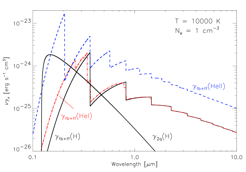
Figure 3: Combined free-bound and free-free continuum for H i (jagged black line), He i (dash-dotted, red), He ii (dashed, blue), and the two-photon continuum for H i (smooth black line), to be compared with fig. 4.1 in Osterbrock & Ferland (2006). Small differences between our data and that of Osterbrock & Ferland (2006) are attributed to the use of recent data from Ercolano & Storey (2006) and van Hoof et al. (2014).

The data for Fig. 3 can be reproduced with the following two commands:

> ./nebular -r 1e13 6e15 1e11 -t 10000 -n 1 -u 2 -k -o out.dat
> awk ’($0!$\sim$/#/) {print $2, $4+$10, $5+$11, $6+$12, $7}’ out.dat > plot.dat

The first command calculates the spectrum. Option -r specifies the frequency range and step size, needed to get the result in frequency units. Option -u 2 specifies that the computations yield the emission coefficients ($\gamma_{\rm fb}$ etc.), i.e. the atomic data tabulated in e.g. Ercolano & Storey (2006), multiplied by frequency $\nu$. Option -k suppresses the calculation of emission lines. A summary of the syntax is given in Table 2.

The second command line is to extract the wavelengths, the sums of free-bound and free-free emission for the three ionic species, and the hydrogen two-photon spectrum, respectively.

A.2 Calculating a model spectrum

Figure 4 shows a model spectrum. The difference to Fig. 3 is that NEBULAR multiplied the various emission coefficients by the electronic and ionic densities. A wavelength range (as compared to a frequency range) is chosen as input, and thus the result is in wavelength units (as opposed to frequency units in the previous example).

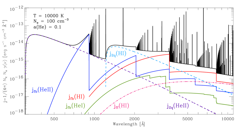
Figure 4: Total emissiion coefficient $j$ for a hydrogen helium gas mix (top thick solid line, including the emission line series). The other three solid lines with the characteristic ionization edges represent the free-bound contributions by H i, He i and He ii. The two dashed lines display the two-photon continua (H i and He ii), and the lower dash-dotted line the H i free-free emission.

The data for Figure 4 were calculated with

> ./nebular -r 300 12000 1 -t 14000 -n 100

If one were to compare this spectrum with a real observation, then it just has to be multiplied with a constant factor (effectively, integrating over the nebula’s volume and folding in the luminosity distance). This would yield the observable spectral flux density, $f_{\lambda}(\lambda)$.

If the observed spectrum is on an arbitrary wavelength scale, then NEBULAR can resample the spectrum on the same grid:

> ./nebular -i <ASCII wavelength table> -t 14000 -n 100

A.3 Visualizing the pseudo-continuum near the Balmer break

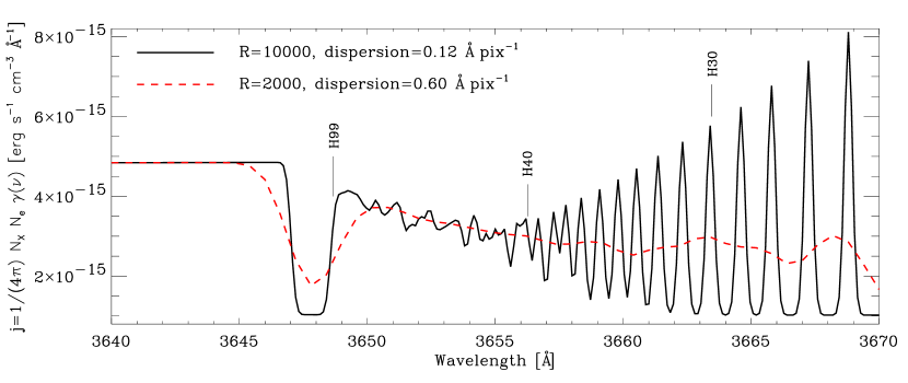
Figure 5: The hydrogen Balmer break at $3646$ Å, as seen by two model spectrographs with resolutions $R=2000$ and $R=10000$, respectively. The confluent high-order Balmer series forms a pseudo-continuum, masking the Balmer break. The broad minimum between 3647 Å and 3649 Å is artificial, because upper levels higher than $n=99$ are not available in NEBULAR.

The data for this plot can be generated by smoothing the model spectrum with a Gaussian kernel, to mimic the finite spectrograph resolution, $R=\lambda/\Delta\lambda$. The FWHM of the kernel is set to $\Delta\lambda$. The spectral dispersion is controlled by the wavelength step size (third numeric argument for option -r). For the $R=10000$ and $R=2000$ examples, dispersions of 0.12 and 0.60 Å$\,{\rm pix}^{-1}$ are used:

> ./nebular -r 3640 3670 0.60 -t 10000 -n 100 -w 1.80 -b -o R2000.dat
> ./nebular -r 3640 3670 0.12 -t 10000 -n 100 -w 0.36 -b -o R10000.dat

Options -w and -b specify the kernel width and suppress the output of header lines, respectively.

Appendix B Corrections to the literature

This is a list of errors (mostly of typographical nature) found in the literature:

• In Table VI of Pengelly (1964) for the He ii Pickering series, for $n=19$, $t^{\prime}=1$ and Case B, it should read 0.39 instead of 3.39.

• Pengelly & Seaton (1964) erroneously have a factor of $\pi^{2}$ in the denominator for the Debye radius (their eq. 33). Correct would be a single factor $\pi$. Subsequent derivations and numeric evaluations, however, are correctly calculated.

• In their eq. (3.40), Brocklehurst (1971) also have a factor of $\pi^{2}$ in the denominator for the Debye radius, and carry it over in their calculations of the collision rates. Spitzer (1956) is cited for the equation, yet in that original work the dependence on $\pi$ is linear. CLOUDY (v13.03) has the same wrong dependence on $\pi^{2}$ in the calculation of the collision rates, a bug that has been fixed in v15.

• In Table 4.2 of Osterbrock & Ferland (2006) the H i Paschen-line series, the values tabulated for $j_{{\rm P}\delta}/j_{{\rm H}\beta}$ actually refer to $j_{{\rm P}\epsilon}/j_{{\rm H}\beta}$. This table has been derived from Pengelly (1964), where this error is absent.

• In Table 4.3 of Osterbrock & Ferland (2006) the relative intensities with respect to He ii$\lambda 4686$ are mistakenly a factor of 10 too low for $n\rightarrow 2$ and $T=5000$, 10000 and 20000 K. This table has been reproduced from Storey & Hummer (1995), where this error is absent.

Appendix C Supplementary tables

Table 2: Command-line arguments for NEBULAR.

Args.	Value	Purpose
-r	min, max, delta [Å  or Hz]	wavelength / frequency range and step size;
		the output will have frequency or wavelength units
-i	input wavelength/frequency table	alternative to -r; ASCII format
-t	electron temperature [K]
-n	electron number density [cm-3]
-f	H+, He+, He++ ion. fractions	optional; calculated internally if omitted
-o	output file name	optional; default: nebular_spectrum.dat
-a	helium abundance ratio by parts	optional; default: 0.10
-c	A or B	optional; Case A/B for emission lines; default: B
-w	FWHM [Å or Hz]	optional; FWHM of a Gaussian kernel to convolve the spectrum
-b	$-$	optional; suppresses header lines if given
-k	$-$	optional; suppresses emission lines if given (faster execution)
-u	0, 1, or 2	0: returns $j=1/(4\pi)\,N_{X}\,N_{e}\,\gamma$ (model spectra)
		1: returns $\gamma$ (atomic data)
		2: returns $\nu\gamma$

Table 3: Resulting output of NEBULAR (abridged). The first two columns contain frequencies and wavelengths. The third column is the total spectrum, either $f_{\nu}$ or $f_{\lambda}$. The remaining columns give the free-bound, two-photon, free-free and emission-line components for H i, respectively (data for He i and He ii are not shown).

$\nu$ [Hz]	$\lambda$ [Å]	$f_{\lambda}$	$j_{\rm fb}$(H i)	$j_{\rm 2q}$(H i)	$j_{\rm ff}$(H i)	$j_{\rm nn^{\prime}}$(H i)
6.16603e+14	4862.0	6.46661e-16	2.92421e-16	2.75241e-16	3.66144e-17	0
6.16578e+14	4862.2	6.46636e-16	2.92431e-16	2.75203e-16	3.66159e-17	0
6.16552e+14	4862.4	6.46612e-16	2.92442e-16	2.75166e-16	3.66174e-17	0
6.16527e+14	4862.6	6.46587e-16	2.92452e-16	2.75128e-16	3.66188e-17	0
6.16502e+14	4862.8	4.42298e-12	2.92463e-16	2.75090e-16	3.66203e-17	4.42234e-12
6.16476e+14	4863.0	6.46538e-16	2.92474e-16	2.75053e-16	3.66218e-17	0
6.16451e+14	4863.2	6.46514e-16	2.92484e-16	2.75015e-16	3.66233e-17	0
6.16426e+14	4863.4	6.46490e-16	2.92495e-16	2.74978e-16	3.66247e-17	0
6.16400e+14	4863.6	6.46465e-16	2.92506e-16	2.74940e-16	3.66262e-17	0
6.16375e+14	4863.8	6.46441e-16	2.92516e-16	2.74902e-16	3.66277e-17	0

Table 4: Effective recombination coefficients to H i $2^{2}$S (upper half) and H i $2^{2}$P (lower half), see also Sect. 2.3. Extracted and reproduced from table 8 in Hummer & Storey (1987). The total recombination coefficient for the $n=2$ level is obtained by adding the $2^{2}$S and $2^{2}$P values.

	${\rm log}\,(N_{e}\,/\,{\rm cm}^{-3})$
	2	3	4	5	6	7	8	9	10
T [K]	$\alpha^{\rm eff}_{{\rm HI}\,2^{2}{\rm S}}[{\rm cm}^{3}\,{\rm s}^{-1}]$
1000	3.594e-13	3.701e-13	3.891e-13	4.226e-13	4.814e-13	5.887e-13	7.959e-13	1.163e-12	1.842e-12
3000	1.843e-13	1.861e-13	1.894e-13	1.950e-13	2.047e-13	2.211e-13	2.491e-13	2.846e-13	3.091e-13
5000	1.334e-13	1.341e-13	1.354e-13	1.377e-13	1.416e-13	1.481e-13	1.592e-13	1.710e-13	1.679e-13
7500	1.020e-13	1.023e-13	1.029e-13	1.039e-13	1.057e-13	1.087e-13	1.137e-13	1.182e-13	1.101e-13
10000	8.373e-14	8.390e-14	8.422e-14	8.477e-14	8.571e-14	8.729e-14	9.006e-14	9.210e-14	8.350e-14
12500	7.152e-14	7.162e-14	7.180e-14	7.213e-14	7.267e-14	7.358e-14	7.525e-14	7.621e-14	6.807e-14
15000	6.268e-14	6.274e-14	6.285e-14	6.305e-14	6.337e-14	6.392e-14	6.497e-14	6.540e-14	5.790e-14
20000	5.059e-14	5.061e-14	5.065e-14	5.072e-14	5.083e-14	5.102e-14	5.147e-14	5.144e-14	4.513e-14
30000	3.690e-14	3.690e-14	3.690e-14	3.689e-14	3.686e-14	3.682e-14	3.687e-14	3.665e-14	3.204e-14
T [K]	$\alpha^{\rm eff}_{{\rm HI}\,2^{2}{\rm P}}[{\rm cm}^{3}\,{\rm s}^{-1}]$
1000	1.151e-12	1.163e-12	1.187e-12	1.235e-12	1.328e-12	1.512e-12	1.912e-12	2.947e-12	5.979e-12
3000	4.854e-13	4.865e-13	4.890e-13	4.943e-13	5.049e-13	5.265e-13	5.703e-13	6.760e-13	9.467e-13
5000	3.185e-13	3.189e-13	3.197e-13	3.216e-13	3.254e-13	3.331e-13	3.489e-13	3.880e-13	4.919e-13
7500	2.251e-13	2.253e-13	2.257e-13	2.265e-13	2.281e-13	2.316e-13	2.386e-13	2.566e-13	3.080e-13
10000	1.747e-13	1.748e-13	1.750e-13	1.755e-13	1.764e-13	1.784e-13	1.823e-13	1.926e-13	2.247e-13
12500	1.429e-13	1.429e-13	1.430e-13	1.434e-13	1.440e-13	1.453e-13	1.478e-13	1.545e-13	1.771e-13
15000	1.208e-13	1.209e-13	1.210e-13	1.212e-13	1.217e-13	1.226e-13	1.243e-13	1.290e-13	1.461e-13
20000	9.220e-14	9.222e-14	9.229e-14	9.243e-14	9.272e-14	9.329e-14	9.425e-14	9.687e-14	1.080e-13
30000	6.217e-14	6.219e-14	6.223e-14	6.231e-14	6.247e-14	6.276e-14	6.319e-14	6.427e-14	7.047e-14

Table 5: Effective recombination coefficients to He ii $2^{2}$S (upper half) and He ii $2^{2}$P (lower half). Extracted and reproduced from table 9 in Hummer & Storey (1987).

	${\rm log}\,(N_{e}\,/\,{\rm cm}^{-3})$
	2	3	4	5	6	7	8	9	10	11	12	13
T [K]	$\alpha^{\rm eff}_{{\rm HeII}\,2^{2}{\rm S}}[{\rm cm}^{3}\,{\rm s}^{-1}]$
3000	8.296e-13	8.373e-13	8.552e-13	8.887e-13	9.487e-13	1.056e-12	1.250e-12	1.627e-12	2.425e-12	4.072e-12	8.155e-12	2.670e-11
5000	6.174e-13	6.207e-13	6.287e-13	6.439e-13	6.712e-13	7.189e-13	8.029e-13	9.551e-13	1.246e-12	1.737e-12	2.632e-12	5.930e-12
7500	4.859e-13	4.876e-13	4.917e-13	4.997e-13	5.140e-13	5.390e-13	5.821e-13	6.578e-13	7.949e-13	9.944e-13	1.272e-12	2.244e-12
10000	4.091e-13	4.101e-13	4.126e-13	4.176e-13	4.265e-13	4.421e-13	4.688e-13	5.149e-13	5.962e-13	7.030e-13	8.167e-13	1.246e-12
12500	3.572e-13	3.578e-13	3.596e-13	3.630e-13	3.691e-13	3.798e-13	3.980e-13	4.292e-13	4.863e-13	5.492e-13	5.996e-13	8.298e-13
15000	3.190e-13	3.195e-13	3.208e-13	3.232e-13	3.277e-13	3.355e-13	3.487e-13	3.713e-13	4.103e-13	4.542e-13	4.748e-13	6.122e-13
20000	2.659e-13	2.661e-13	2.669e-13	2.683e-13	2.710e-13	2.756e-13	2.835e-13	2.968e-13	3.197e-13	3.423e-13	3.381e-13	3.961e-13
30000	2.036e-13	2.037e-13	2.041e-13	2.047e-13	2.059e-13	2.080e-13	2.116e-13	2.176e-13	2.281e-13	2.361e-13	2.199e-13	2.313e-13
50000	1.430e-13	1.430e-13	1.431e-13	1.433e-13	1.437e-13	1.443e-13	1.454e-13	1.473e-13	1.508e-13	1.519e-13	1.352e-13	1.289e-13
100000	8.524e-14	8.524e-14	8.525e-14	8.526e-14	8.529e-14	8.531e-14	8.535e-14	8.541e-14	8.584e-14	8.512e-14	7.384e-14	6.482e-14
T [K]	$\alpha^{\rm eff}_{{\rm HeII}\,2^{2}{\rm P}}[{\rm cm}^{3}\,{\rm s}^{-1}]$
3000	2.830e-12	2.844e-12	2.866e-12	2.908e-12	2.995e-12	3.168e-12	3.516e-12	4.244e-12	5.888e-12	1.051e-11	2.671e-11	9.972e-11
5000	1.926e-12	1.931e-12	1.938e-12	1.953e-12	1.985e-12	2.047e-12	2.174e-12	2.433e-12	2.983e-12	4.390e-12	8.497e-12	2.206e-11
7500	1.407e-12	1.409e-12	1.412e-12	1.418e-12	1.432e-12	1.460e-12	1.516e-12	1.631e-12	1.869e-12	2.459e-12	4.036e-12	8.288e-12
10000	1.121e-12	1.123e-12	1.124e-12	1.127e-12	1.135e-12	1.150e-12	1.181e-12	1.246e-12	1.378e-12	1.706e-12	2.551e-12	4.567e-12
12500	9.375e-13	9.383e-13	9.392e-13	9.411e-13	9.457e-13	9.553e-13	9.753e-13	1.016e-12	1.101e-12	1.310e-12	1.846e-12	3.017e-12
15000	8.082e-13	8.088e-13	8.093e-13	8.106e-13	8.136e-13	8.202e-13	8.340e-13	8.624e-13	9.205e-13	1.067e-12	1.442e-12	2.209e-12
20000	6.366e-13	6.369e-13	6.371e-13	6.378e-13	6.394e-13	6.430e-13	6.507e-13	6.666e-13	6.989e-13	7.828e-13	1.001e-12	1.407e-12
30000	4.502e-13	4.503e-13	4.504e-13	4.507e-13	4.514e-13	4.529e-13	4.563e-13	4.633e-13	4.774e-13	5.161e-13	6.232e-13	7.972e-13
50000	2.857e-13	2.858e-13	2.858e-13	2.859e-13	2.862e-13	2.868e-13	2.880e-13	2.907e-13	2.955e-13	3.102e-13	3.570e-13	4.215e-13
100000	1.488e-13	1.488e-13	1.488e-13	1.488e-13	1.489e-13	1.491e-13	1.495e-13	1.503e-13	1.515e-13	1.552e-13	1.720e-13	1.912e-13

References

- Brocklehurst (1971) Brocklehurst, M. 1971, MNRAS, 153, 471
- Brown & Mathews (1970) Brown, R. L. & Mathews, W. G. 1970, ApJ, 160, 939
- Drake et al. (1969) Drake, G. W., Victor, G. A., & Dalgarno, A. 1969, Physical Review, 180, 25
- Ercolano & Storey (2006) Ercolano, B. & Storey, P. J. 2006, MNRAS, 372, 1875
- Ferland et al. (2013) Ferland, G. J., Porter, R. L., van Hoof, P. A. M., et al. 2013, Rev. Mexicana Astron. Astrofis., 49, 137
- Golovatyj et al. (1997) Golovatyj, V. V., Sapar, A., Feklistova, T., & Kholtygin, A. F. 1997, Astronomical and Astrophysical Transactions, 12, 85
- Guzmán et al. (2016) Guzmán, F., Badnell, N. R., Williams, R. J. R., et al. 2016, MNRAS
- Hirata (2008) Hirata, C. M. 2008, Phys. Rev. D, 78, 023001
- Hummer & Storey (1987) Hummer, D. G. & Storey, P. J. 1987, MNRAS, 224, 801
- Laporte & Meggers (1925) Laporte, O. & Meggers, W. F. 1925, Journal of the Optical Society of America, 11, 459
- Lintott et al. (2009) Lintott, C. J., Schawinski, K., Keel, W., et al. 2009, MNRAS, 399, 129