Tristable and multiple bistable activity in complex random binary networks of two-state units

Abstract

We study complex networks of stochastic two-state units. Our aim is to model discrete stochastic excitable dynamics with a rest and an excited state. Both states are assumed to possess different waiting time distributions. The rest state is treated as an activation process with an exponentially distributed life time, whereas the latter in the excited state shall have a constant mean which may originate from any distribution. The activation rate of any single unit is determined by its neighbors according to a random complex network structure. In order to treat this problem in an analytical way, we use a heterogeneous mean-field approximation yielding a set of equations general valid for uncorrelated random networks. Based on this derivation we focus on random binary networks where the network is solely comprised of nodes with either of two degrees. The ratio between the two degrees is shown to be a crucial parameter. Dependent on the composition of the network the steady states show the usual transition from disorder to homogeneous ordered bistability as well as new scenarios that include inhomogeneous ordered and disordered bistability as well as tristability. The various steady states differ in their spiking activity expressed by a state dependent spiking rate. Numerical simulations agree with analytic results of the heterogeneous mean-field approximation.

1 Introduction

Discrete-state stochastic models can be used to describe discrete processes such as the orientation of a spin or the blinking of quantum dots Frantsuzov09 . Additionally, systems with continuously changing dynamics can be mapped to discrete-state descriptions via coarse-graining Lindner2004 ; HuberTsim2005 ; PikovskyTsim2001 . Despite the simplicity of the single units, the collective effects of ensembles of coupled units can be highly non-trivial.

In earlier works discrete stochastic three-state models have been used to investigate fluctuation driven spin nucleation on complex networks Chen15 . Two- and three-state models have been applied to neuronal systems Dumont2014 ; PrFaSchiZa07 and recently to language dynamics Colaiori15 . Synchronization behavior, phase transitions and reaction to time delayed feedback WoodLind06 ; WoodLind07 ; WoodLind06PRE ; Prager2003 ; EscaffLind12 ; Kouvaris2010 ; HuberTsim2005 ; PikovskyTsim2001 as well as excitability Prager2007 ; Leonhardt2008 are general aspects that apply to a wide range of natural phenomena.

Most of the referenced works consider Markovian – thereby memoryless – discrete-state models WoodLind06 ; WoodLind07 ; WoodLind06PRE ; Pinto2014 . A disordered environment Trimper04 or the reduction of models with a high number of discrete states to a model with fewer states generically demands a non-Markovian description. Therefore, in continuation of previous work Prager2003 ; PrFaSchiZa07 ; Prager2007 in this paper a semi-Markovian model cox1962renewal of stochastic two-state units is considered. As a new point of interest these units are embedded in an uncorrelated random network whose nodes possess different but independent degrees, in particular this excludes networks with high asortativity or dissortativity. The structure of the network is given by the node distribution $p(k)$. A big number of nodes is assumed, it is known that finite size effects Pinto2014 have a strong effect on the dynamic of the stochastic process as well as on the network influence. Complex networks are of top interest in statistical physics because it allows deviation from global coupling without specification of a spatial structure as well as providing a framework to map complex spatial structures to an abstract space. Furthermore, network structures are present in many situations of everyday life, for example transport Barrat2004 ; Jiang2007 ; Mukherjee2003 and supply networks Runions2005 to mention just a few.

The paper is structured as follows. In Section 2 the master equations for stochastic two-state units are derived. In Section 2.3 the heterogeneous mean-field approximation is used to reduce the set of equations. Section 3 applies the formalism to random binary networks and consists of three subsections. In the first subsection the implicit equations for the steady states are derived and analyzed for saddle-node bifurcations. From this, the scaling of the critical coupling strength due to the network embedding is revealed. The second subsection addresses the limit of vanishing noise. Finally, the last subsection shows the results of the numerical solutions of the mean-field equations in presence of finite noise. Apart from the expected homogeneous ordered bistability that is known from globally coupled units Prager2003 ; PrFaSchiZa07 , inhomogeneous ordered and disordered states as well as tristable states are uncovered. These findings are confirmed via microscopic simulations using the original network structure. In these simulations the network exhibits a variable firing activity by approaching different steady states in dependence on the initial conditions. But the firing of the populations is not synchronized and thus the mean-field stays constant. The firing differs in the spike generating rates for the two populations and whether these are in the rest or excited states. The spike time statistics of individual units are discussed separately. Given that the excited state possess an exponentially distributed waiting time, the spike trains are always nearly Poissonian. For a sharp-peaked waiting time density with no variance, the spike trains become highly coherent.

2 Two-state processes on complex networks

2.1 Master equation of coupled two-state units

The stochastic two-state units considered in this work can switch between the states $0$ and $1$. They do so in a stochastic fashion, governed by the waiting time distributions $w_{0,i}(t)$ and $w_{1}(t)$ in the corresponding states, as explained Fig. 1. Focusing on excitable dynamics, state $0$ will be called the resting state and state $1$ the excited state.

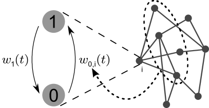
Figure 1: Sketch of the considered units and their topology. The two-state units with the waiting-time distributions $w_{0,i}(t)$ and $w_{1}(t)$ are embedded in a binary random network, as indicated by the dashed lines. In this example are five nodes with degree two and four nodes with degree four. The highlighted unit $i$ is one of the latter, hence its activation waiting-time distribution $w_{0,i}(t)$ is affected by the activity of four neighbors, as indicated by the dotted ellipse and the dotted arrow.

In this way, the transition from rest to excited, i.e. from state $0$ to state $1$, will be assumed as an activation process. The life time in state $0$ is exponentially distributed and the state will be left with the transition rate $\gamma$.

The backward transition (relaxation from excited to rest) is governed by the waiting time density $w_{1}(t)$ to remain in state $1$. So far this density is arbitrary except that its mean value shall be $\tau$ and does not depend on any other parameters such as the noise intensity, the size and structure or possible dynamical states of the network. In the simulations two specific choices are made. First, the relaxation is treated as a Markovian rate process with a exponential waiting time distribution

$$w_{1}(t)=\frac{1}{\tau}\exp\left(-\frac{t}{\tau}\right).$$ (1)

Oppositely, when modeling excitable dynamics, a sharply peaked distribution is more suitable, e.g.

$$w_{1}(t)=\delta(t-\tau)$$ (2)

would yield a constant waiting time without any variance in state $1$ modeling a fixed delay Prager2003 ; Prager2007 ; Kouvaris2010 . As shown in the appendix A, the bifurcations of the steady states are not affected by the specific choice of $w_{1}$. It depends on the mean time $\tau$ spent in the excited state. Only, setups with possible transition to a non-stationary behavior reflect on the choice of $w_{1}$.

The two-state units are located on the $N$ nodes of a complex network. Each stochastic element receives the output from the units to which it is linked in the network by edges. This coupling is mathematically realized by introduction of the adjacency matrix $\mathsf{A}$. The activation rate $\gamma_{i}$ from state $0$ to state $1$ of the $i$th node $i\in\{1,\dots,N\}$ is assumed to depend on a signal function $f_{i}(t)$

$$\gamma_{i} =\gamma[f_{i}(t)],$$ (3)

which contains the adjacency matrix

$$f_{i}(t) =\frac{1}{N}\,\sum_{j=1}^{N}A_{ij}\,s_{j}(t).$$ (4)

Therein, $s_{j}(t)$ is the output signal of node $j$ depending on its state. In this work, undirected and unweighted networks are considered, hence the adjacency matrix is symmetric with elements $A_{ij}=1$, if the units $i$ and $j$ are connected, otherwise $A_{ij}=0$.

Typically, excitable systems stay in the resting state where no output is produced. Upon sufficient excitation they drastically change their intrinsic dynamics which is emitted as a signal. Here such “spiking” is modeled by a two-valued output function $s_{j}(t)$, which can take the values $1$ in the excited state and $0$ otherwise. This setting is motivated by neuronal activity or excitable lasers. A symmetric choice would be more appropriate in order to model magnetic spins.

Eventually, in accordance with previous assumptions, the normalized waiting time distribution density of the activation with the time dependent rate from (4) is given by the exponential function

$$w_{0,i}(t)=\gamma[f_{i}(t)]\,\exp\left(-\int_{0}^{t}\,\gamma[f_{i}(t^{\prime})]\,\mathrm{d}t^{\prime}\right).$$ (5)

Let $P_{i}(0,t)$ denote the occupation probability of unit $i$ to be in state $s_{i}(t)=0$ at time $t$. Analogously $P_{i}(1,t)$ for state $s_{i}(t)=1$. Then the balance of probability flows yields the generalized master equations

$$\dot{P}_{i}(0,t) =-J_{0\rightarrow 1,i}(t)+J_{1\rightarrow 0,i}(t),$$ (6)

$$\dot{P}_{i}(1,t) =-J_{1\rightarrow 0,i}(t)+J_{0\rightarrow 1,i}(t),$$

for all $i\in\{1,\dots,N\}$, where $J_{0\rightarrow 1,i}(t)$ gives the probability flow from state $0$ to $1$ of unit $i$ at time $t$. Since the transition $0\rightarrow 1$ is a rate process, its probability flow is simply given by

$$J_{0\rightarrow 1,i}(t)=\gamma[f_{i}(t)]P_{i}(0,t).$$ (7)

The second probability flow is given by all the probability that has flown into state $1$ up to time $t$ and stayed there for a time, which is given by the waiting time distribution $w_{1}(t)$. Thus it is the convolution of $J_{0\rightarrow 1,i}(t)$ and $w_{1}(t^{\prime})$,

$$J_{1\rightarrow 0,i}(t)=\int_{0}^{\infty}\gamma[f_{i}(t-t^{\prime})]P_{i}(0,t-t^{\prime})w_{1}(t^{\prime})\mathrm{d}t^{\prime}.$$ (8)

Using the normalization condition at a given node

$$P_{i}(0,t)=1-P_{i}(1,t),$$ (9)

the temporal evolution of the occupation probabilities $P_{i}(1,t)$ is then given by (cf. (6))

$$\dot{P}_{i}(1,t)=\gamma[f_{i}(t)](1-P_{i}(1,t))-$$

$$-\int_{0}^{\infty}\gamma[f_{i}(t-t^{\prime})](1-P_{i}(1,t-t^{\prime}))w_{1}(t^{\prime})\mathrm{d}t^{\prime},$$

$$\hskip 105.2751pti\in\{1,\dots,N\}.$$ (10)

This is a set of $N$ coupled linear integro-differential equations for the $P_{i}(1,t)$. The complexity is given by the chosen adjacency matrix $A_{i,j}$ which links the almost $N$ equations by the the signal function, see Eq. (4).

By applying a heterogeneous mean-field approximation as described in Section 2.3, the structure of this set of equations is much simpler and the number of differential equations in the set reduces significantly. As consequence of this approximation, the set will become analytically treatable for special cases in the stationary limit.

But before describing this approximation, an appropriate notation for the values describing the dynamical behavior on a complex network will be introduced.

2.2 Master equation on complex networks

To include the network topology into the description, it is assumed that the complex network structure can be described as a random network. Central value in this description are the degrees $k_{i}$ of the $N$ nodes. For a given adjacency matrix $A_{i,j}$ with values $0,1$ the degree $k_{i}$ of the $i$th node is the number of existing links to other nodes of the network. It becomes

$$k_{i}=\sum_{j=1}^{N}A_{i,j}.$$ (11)

Let $k_{\mathrm{min}}$ and $k_{\mathrm{max}}$ be the minimum and maximum degree occurring in the network, respectively, while $N_{k}$ is the number of units with degree $k\in[k_{\mathrm{min}},k_{\mathrm{max}}]$. In a random network the degrees can be treated as random numbers. Their occupation probability $p(k)$ is defined by $N_{k}$. Then the occupation probability reads

$$p(k)=\lim_{N\to\infty}\frac{N_{k}}{N}.$$ (12)

Mathematically, the limit make sense if $N_{k}~{}\propto~{}N$. Afterwards, sorting the nodes with coinciding degrees $k$ in the network gives the joint probability that any node in the network has this degree and is, respectively, in the dynamical state $s=(0,1)$ at time $t$

$$P(s,k,t)=\sum_{i=1}^{N}\,\delta_{s,s_{i}}\,\delta_{k,k_{i}}\,P_{i}(s_{i},k_{i},t).$$ (13)

Using Bayes’ theorem we split off the occupation probability $p(k)$ as

$$P(s,k,t)=P(s,t|k)p(k).$$ (14)

Normalization reads

$$P(0,k,t)\,+\,P(1,k,t)=p(k).$$ (15)

Hence, for the conditioned probabilities the degree is fixed and it becomes

$$P(0,t|k)\,+\,P(1,t|k)=1.$$ (16)

The chosen conditional probabilities $P(1,t|k)$ neglect that various nodes with the same degree $k$ might be linked to $k$ nodes with different degrees. Therefore, without a further approximation, they are so far not suitable for the description of our situation.

To proceed, the signal function (4) which is coupling the $i$th node to the other nodes will be considered now. Replacing therein the number of the linked node $j$ by the specific degree $k_{j}$ of this node, it becomes

$$f_{i}(t)=\frac{1}{N}\,\sum_{j=1}^{N}\,A_{i,j}s_{k_{j}}(t).$$ (17)

Sorting different degrees gives

$$f_{i}(t)=\sum_{k=k_{min}}^{k_{max}}\,\frac{N_{k}}{N}\,\frac{1}{N_{k}}\,\sum_{j=1}^{N}\,\delta_{k,k_{j}}\,A_{i,j}\,s_{k_{j}}(t).$$ (18)

Every node receives its input depending on the specific linked environment. Due to the disorder contained in the adjacency matrix $A_{i,j}$, the summation is still in general different for distinct nodes. The reduced description for given degrees requires an additional approximation.

2.3 Heterogeneous mean-field approximation

As proposed in Ichinomiya2004 ; Sonnenschein2012 ; Carro2016 , the complex network with the adjacency matrix $A_{i,j}$ and with the given degree distribution $p(k)$ will be replaced by a fully connected network with weighted edges. The latter with adjacency matrix $\tilde{A}_{i,j}$ shall possess the same distribution of the degrees at the nodes. In detail, it is required that the degree-values of all nodes in the new network shall coincide with the corresponding ones in the original network. Accordingly, the following shall hold

$$\sum_{j=1}^{N}A_{i,j}\,=\,k_{i}\,=\sum_{j=1}^{N}\tilde{A}_{i,j}.\quad i=1,\ldots,N.$$ (19)

Whereas the sum at the l.h.s. is running over values $1$ and $0$ of $A_{i,j}$, at the r.h.s. the sum goes over rational numbers. The assumption is made that the probability to have an edge between the $i$th and $j$th node is proportional to the product of the degrees of these nodes, i.e., to $k_{i}\,k_{j}$. This is strictly valid only for uncorrelated networks. Further on, taking into account the conservation of degree as required in (19) the following replacing for a fully connected network is defined

$$\tilde{A}_{ij}=\frac{k_{i}\,k_{j}}{\sum_{l=1}^{N}k_{l}}.$$ (20)

Figure 2 illustrates the replacement. As a result the single nodes with given degree $k$ couple uniquely to a mean filed. Hence, in contrast to the original network, the fully connected network will allow a mean-field representation with respect to all edges with coinciding degrees $k$. In Sonnenschein2012 the validity of this replacement procedure was discussed and it was successfully applied to complex networks with continuous phase oscillators at the nodes. The approach Ichinomiya2004 ; Sonnenschein2012 ; Carro2016 is here generalized to discrete stochastic two state units.

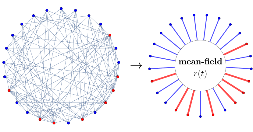
Figure 2: Representation of a random binary network with $k_{1}=12$, $k_{2}=6$ and $N=25$ before and after applying the heterogeneous mean-field approximation.

As a result of the replacement, the signal function in (18) is approximated as

$$\tilde{f}_{i}(t)\approx\frac{1}{N}\sum_{j=1}^{N}\tilde{A}_{ij}s_{j}(t)=\frac{k_{i}}{N\sum_{l=1}^{N}k_{l}}\sum_{j=1}^{N}k_{j}s_{j}(t).$$ (21)

It follows immediately, that the signal at the node with degree $k_{i}$ coincides for all nodes with the same degree. The node value itself enters only multiplicatively into this expression. Hence, the denominator of the sum is equal for all nodes.

Crossing from the summation over all nodes to sums with the same degrees similar transformations as above are made. The different degrees $k_{i}$ are again divided into classes of units with the same degree $k$ and with occupation number $N_{k}$. Obviously, $\sum_{k=k_{\mathrm{min}}}^{k_{\mathrm{max}}}N_{k}=N$ has to be satisfied. The denominator can be rewritten

$$\sum_{j=1}^{N}k_{j}=\sum_{k=k_{\mathrm{min}}}^{k_{\mathrm{max}}}N_{k}k.$$ (22)

In the limit of large number of nodes ${N\to\infty}$ this expression becomes $N\langle k\rangle$ where the symbol $\langle\cdot\rangle=\sum_{k}\;\cdot\;p(k)$ assigns averaging over the degree distribution.

Hence, the signal function of the $i$th node becomes

$$f_{i}(t)=\frac{k_{i}}{N}r(t).$$ (23)

Therein, the mean-field amplitude $r(t)$ is defined by

$$r(t)=\frac{1}{\langle k\rangle}\,\sum_{k=k_{\mathrm{min}}}^{k_{\mathrm{max}}}\,\frac{N_{k}}{N}\,k\,\frac{1}{N_{k}}\sum_{j=1}^{N}\,\delta_{k_{,}k_{j}}\,{s}_{k_{j}}(t).$$ (24)

It is assumed that, after forgetting initial conditions, units with the same degree share stochastic pulse sequences which are statistically identical. Therefore, the same pulse sequence can be assigned to units of the same degree class by taking the average over the corresponding class

$$\overline{s}_{k}(t)=\frac{1}{N_{k}}\sum_{j=1}^{N}\,\delta_{k,k_{j}}\,s_{k_{j}}(t).$$ (25)

Therein, the sum runs over $N_{k}$ items due to the action of the $\delta$-function. Since the number of nodes with degree $k$ scales as $N_{k}\propto N$, application of the limit of large $N$ yields

$$\lim_{N\to\infty}\overline{s}_{k}(t)=P(1,t|k),$$ (26)

which was introduced in (14).

Thus, the mean-field $r(t)$ introduced in (24) becomes in this limit

$$r(t)=\frac{1}{\langle k\rangle}\sum_{k^{\prime}=k_{\mathrm{min}}}^{k_{\mathrm{max}}}p(k^{\prime})k^{\prime}P(1,t|k)=\frac{\langle k\,P_{1,k}(t)\rangle}{\langle k\rangle}.$$ (27)

Eventually, by inserting (23) and (24) via (27) into the mean-field description (15) and (10) the following expression is obtained

$$P(0,t|k)=1-P(1,t|k),$$ (28)

$$\dot{P}(1,t|k)=\gamma\left[\frac{k}{N}r(t)\right]\left(1-P(1,t|k)\right)-$$

$$\int_{0}^{\infty}\gamma\left[\frac{k}{N}r(t-t^{\prime})\right]\left(1-P(1,t-t^{\prime}|k)\right)w_{1}(t^{\prime})\mathrm{d}t^{\prime}.$$

This is now a set of coupled non-linear integro-differential equations, since the mean-field $r(t)$ depends on $P(1.t|k)$ via (27). Though the structure of the equations looks similar to the previous Master equation (10) it is qualitatively different. As the result of the replacement of the adjacency matrix, the number of equations has reduced drastically compared to the system (15) and (10). The index $k$ in (28) is only running over the different possible degrees in the network $k\in[k_{\mathrm{min}},k_{\mathrm{max}}]$ whereas in (15) and (10) it runs over all nodes $N$. In addition, the dependence of the activation rate $\gamma$ on the degree $k$ appears uniquely in the argument for all nodes as linear factor in the signal function, cf. (23). In the master equation for nodes with the degree $k$ it reads

$$\gamma[f]=\gamma\left[\frac{k}{N}r(t)\right].$$ (29)

2.4 Stationary behavior of excitable units

Depending on the specific structure of $\gamma$ this equation can be highly non-linear. Here in this manuscript, the activation rate $\gamma$ is assumed to follow Arrhenius’ law Rice1954 ; Hanggi1990 . The two-state system shall mimic the behavior of stochastic excitable dynamics Lindner2004 with state $0$ being the rest state and state $1$ the excited one, respectively. Transitions to the excited state $1$ is achieved by overcoming a threshold with barrier $\Delta U$ under the influence of noise with intensity $D$. The corresponding Arrhenius’ law of the rate reads

$$\gamma=\gamma_{0}\,\exp\left(-\frac{\Delta U}{D}\right),$$ (30)

with a constant $\gamma_{0}$ defining the time scale.

The coupling between units is assumed to be purely excitatory and thus each coupled unit that is already in the excited state will lower the potential barrier by an amount proportional to the coupling strength $\sigma$, which is the same for every unit throughout this paper. The following ansatz for the potential $\Delta U$ combines the above information

$$\Delta U=1-\sigma\,\frac{k}{N}r(t).$$ (31)

Setting $p(k)=\delta_{k,N}$ restores the globally connected network with $r(t)\rightarrow P(1,t|N)$, which has been earlier studied in detail Kouvaris2010 . Alternatively, it is possible to consider a discrete number of $K$ degrees $k_{i}$, $i=1,\dots,K$. The corresponding degree distribution follows as

$$p(k)=\sum_{i=1}^{K}\,\nu_{i}\,\delta_{k_{i},k}$$ (32)

Insertion of the specific rate and degree distribution (28) yields a set of $K$ nonlinear master equations. A qualitative discussion of the possible stationary solutions $P^{*}(1|k_{i})$ which will be approached as $t\to\infty$ will be outlined. Since the equations are nonlinear there might exist a different number of stationary solutions with different stability. If distributed by (32) and with the rate function (31) these stationary states are defined by the set of $K$ coupled nonlinear algebraic equations

$$P^{*}(1|k_{i})\, =\,\frac{\tau\gamma_{i}^{*}}{1+\tau\gamma_{i}^{*}},$$ (33)

with the stationary spiking rates of the elements with degree $k_{i}$

$$\gamma_{i}^{*} =\gamma\left[\frac{k_{i}}{N}\,r^{*}\right]$$ (34)

and the stationary mean-field amplitude with (33) inserted and averaged over the discrete distribution (32)

$$r^{*} =\frac{1}{\langle k\rangle}\,\left\langle k\,P^{*}(1|k)\right\rangle.$$ (35)

The maximal number of possible stable solutions of this set of equations can be estimated to be of the order $O(2^{K})$. The behavior is similar to a spin chain with $K$ elements. Every population is stable in the rest state $s_{i}=0$. If being coupled, every population with given degree reaches a stationary probability to be in the excited state.

The precise number depends on the specific degree values, the noise intensity $D$ and the coupling constant $\sigma$. Generally for low coupling, respectively for high noise only a single solution exists, which is the disordered state of all populations. Lowering of noise, respectively increasing coupling, enlarges the number with multiple stable states, including inhomogeneous cases and the two homogeneous situations where all populations are in the rest or in the excited states. In general, it depends on the initial conditions which state will be populated.

Corresponding to the selected steady-state-solution the spiking rates differ. The spiking rate from rest to excited is determined by the stationary states of the population which the element belongs to. It is expressed by the rate given in (34) where the specific solution has to be inserted. Such state dependent dynamical behavior of neuronal activity was recently discussed for phase oscillators in Kromer2014 .

In this simplified model no Hopf-bifurcation can take place. All interactions have an aligning effect of the elements similar to a spin chain. Therefore, the existence of stable oscillating, chimaera state, cluster synchronization or chaotic solutions can be excluded. But adding delayed feedback of the mean-field, mixtures of excitatory and inhibitory acting units of the network or systematic shifts in the signal function might be a source for more complex situations.

Special initial conditions (for example all units in the excited state) cause damped oscillations of the mean-field. Even in the case of a $\delta$-function as waiting time density, the assumed exponentially distributed activation times scatter the individual spins with large dispersion. Hence the coherence of special initial conditions is destroyed after a few excitations yielding a stationary mean-field.

Nevertheless, as will be seen in the next section, the individual spins can fire with a small CV resembling oscillatory behavior. In the states with high mean-field values the activation time becomes negligible small. In these situations the spiking is dominated by the recovery time from the excited to the rest state. If this time does not possess remarkable dispersion the CV become vanishingly smalls.

In the next Section 3 further insight into the consequences of several degrees will be given by dealing with the simplest case of network with two populations with different degrees $k_{1},k_{2}$, only.

3 Random binary networks

In the following, the properties of a binary random network Lambiotte2007 ; Sonnenschein2013 ; Carro2016 will be studied. It allows a full sketch of the possible bifurcation scenario appearing in these networks. These ones are randomly connected with two different degrees $k_{1}$ and $k_{2}$.

In terms of the degree distribution for a binary network it is supposed that

$$p(k)=\nu\delta_{k,k_{1}}+(1-\nu)\delta_{k,k_{2}}.$$ (36)

where $\nu\in]0,1[$ is the fraction of nodes with degree $k_{1}$. In this paper $k_{1}>k_{2}$ is set, but due to the symmetry $(k_{1},\nu)\longleftrightarrow(k_{2},1-\nu)$ the alternative case is also included.

The set of two master equations for binary networks read:

$$\dot{P}(1,t|k_{1})=\gamma_{k_{1}}(t)\;(1-P(1,t|k_{1})-$$

$$\int_{0}^{\infty}\gamma_{k_{1}}(t-t^{\prime})(1-P(1,t-t^{\prime}|k_{1}))w_{1}(t^{\prime})\mathrm{d}t^{\prime},$$

$$\dot{P}(1,t|k_{2})=\gamma_{k_{2}}(t)\;(1-P(1,t|k_{2}))-$$

$$\int_{0}^{\infty}\gamma_{k_{2}}(t-t^{\prime})(1-P(1,t-t^{\prime}|k_{2}))w_{1}(t^{\prime})\mathrm{d}t^{\prime},$$ (37)

where we have denoted $\gamma_{k_{1}}(t)=\gamma[k_{1}/Nr(t)]$ and $\gamma_{k_{2}}(t)$, respectively. Equations (37) can be brought into the integral form phdKouvaris :

$$P (1,t|k_{1})=$$

$$\int_{0}^{\infty}\gamma_{k_{1}}(t-t^{\prime})(1-P(1,t-t^{\prime}|k_{1}))z_{1}(t^{\prime})\mathrm{d}t^{\prime},$$

$$P (1,t|k_{2})=$$

$$\int_{0}^{\infty}\gamma_{k_{2}}(t-t^{\prime})(1-P(1,t-t^{\prime}|k_{2}))z_{1}(t^{\prime})\mathrm{d}t^{\prime},$$ (38)

supplemented by initial conditions. Therein, $z_{1}(t)$ is the survival probability of state $1$,

$$z_{1}(t)=1-\int_{0}^{t}w_{1}(t^{\prime})\mathrm{d}t^{\prime}.$$ (39)

Equations (38) have to be supplemented by initial conditions.

3.1 Qualitative discussion of steady states

Equations (38) are suitable for calculating the steady states of this system. For a steady state $\lim_{t\rightarrow\infty}P(1,t|k_{i})=P^{*}(1|k_{i})$ applies. Using (38) and integration by parts gives the following coupled implicit equations for the steady states

$$P^{*}(1|k_{1}) =\frac{\tau\gamma_{k_{1}}^{*}}{1+\tau\gamma_{k_{1}}^{*}},\qquad P^{*}(1|k_{2})=\frac{\tau\gamma_{k_{2}}^{*}}{1+\tau\gamma_{k_{2}}^{*}}.$$ (40)

The values of $P^{*}(1|k_{1})^{*}$ and $P^{*}(1|k_{2})^{*}$ define the stationary order in the two subpopulations. In Eq. (40) we introduced the mean relaxation time of the excited state $\tau=\int_{0}^{\infty}t\,w_{1}(t)\mathrm{d}t$ and the steady state activation rate $\gamma^{*}_{k_{i}}=\gamma[k_{i}r^{*}]$ for $i=1,2$ depending on the steady state mean-field $r^{*}$. Equation (27) defines the order parameter of the full network. It becomes $r^{*}=\left\langle kP^{*}(1|k)\right\rangle/\langle k\rangle$. Taken at steady state, this yields a transcendent equation for the steady state value $r^{*}$ of the mean-field which yields

$$r^{*}=\frac{1}{\langle k\rangle}\left\langle\frac{k}{1+\frac{1}{\tau\gamma_{k}^{*}}}\right\rangle.$$ (41)

This equation can possess several solutions which we will discuss in detail, later on. In case of large noise $D\to\infty$, only the homogeneous disordered solution $r^{*}=1/2$ exists. In this limit the exponential function becomes unity and since we will select $\gamma_{0}\tau\approx 1$ the disordered state is characterized by $r^{*}=1/2$. A constant value of $r^{*}$ does not imply that the activity of the individual nodes has ceased. It is rather the mean activity or flow that is constant (cf. Fig. 8). Oscillating behavior of $r^{*}$ would correspond to synchronization among the units. But without further ingredients like delayed feedback or additional inhibitory coupled nodes such states cannot be reached.

The transition to the disordered state can be studied in more detail. Demanding that the first derivatives of l.h.s. and r.h.s. with respect to $r$ coincide at $r=r^{*}$ , provides a condition for a saddle-node bifurcation. The homogeneous disordered state becomes unstable and two new stable solutions occur.

Execution of the derivatives in (41) results in

$$\frac{k_{1}\nu}{\langle k\rangle}\frac{\tau\;\frac{\partial\gamma_{k_{1}}^{*}}{\partial r^{*}}}{(1+\gamma_{k_{1}}^{*}\tau)^{2}}+\frac{k_{2}(1-\nu)}{\langle k\rangle}\frac{\tau\;\frac{\partial\gamma_{k_{2}}^{*}}{\partial r^{*}}}{(1+\gamma_{k_{2}}^{*}\tau)^{2}} =1.$$ (42)

Using (40) this becomes

$$1=\frac{k_{1}\nu}{\langle k\rangle}(P^{*}(1|k_{1})-(P^{*}(1|k_{1}))^{2})\frac{\partial\log(\gamma_{k_{1}}^{*})}{\partial r^{*}} +$$

$$\frac{k_{2}(1-\nu)}{\langle k\rangle}(P^{*}(1|k_{2})-(P^{*}(1|k_{2}))^{2})\frac{\partial\log(\gamma_{k_{2}}^{*})}{\partial r^{*}}$$ . (43)

Changing the variables to $x_{k_{1}}:=P^{*}(1|k_{1})-\frac{1}{2}$ and $x_{k_{2}}:=P^{*}(1|k_{2})-\frac{1}{2}$ and rearranging the equation gives

$$\frac{x_{k_{1}}^{2}}{a_{1}^{2}}+\frac{x_{k_{2}}^{2}}{a_{2}^{2}} =1.$$ (45)

Equation (45) defines an ellipse with semi-axes

$$a_{1}=\frac{1}{2}\sqrt{\frac{\big{\langle}k\frac{\partial\log(\gamma^{*}_{k})}{\partial r^{*}}\big{\rangle}-4\langle k\rangle}{k_{1}\nu\frac{\partial\log(\gamma_{k_{1}}^{*})}{\partial r^{*}}}}$$ (46)

and similarly $a_{2}$ with the substitutions$k_{1}\rightarrow k_{2}$ and $\nu\rightarrow(1-\nu)$. The ellipse reduces to a point where the two bifurcations merge. It corresponds to $P^{*}(1|k_{1})~{}=~{}P^{*}(1|k_{2})~{}=~{}r^{*}~{}=~{}\frac{1}{2}$, at

$$\left\langle k\frac{\partial\log(\gamma^{*}_{k})}{\partial r^{*}}\right\rangle-4\langle k\rangle=0.$$ (47)

For the $\gamma_{k}$ given by (31), (47) results in

$$\frac{\sigma_{\text{crit}}}{4D_{\text{crit}}}\frac{\langle k^{2}\rangle}{N\,\langle k\rangle}=1.$$ (48)

Comparing this to the well known result of all-to-all coupled stochastic two-state units Kouvaris2010 ,

$$\frac{\sigma_{\text{crit}}}{4D_{\text{crit}}}=1,$$ (49)

it is visible that it differs only by a scaling factor given by the ratio of the first two moments of the degree (density) distribution. This is a typical network effect in mean-field coupled oscillators Restrepo2005 ; ArenasKuths08 ; Boccaletti06 ; Newman03 . The factor can be interpreted as the mean of the degree distribution of the nearest neighbors Dorogovtsev02 assuming that the local structure of the network is treelike. Therefore the effective coupling strength

$$\sigma_{\rm eff}=\sigma\frac{\langle k^{2}\rangle}{\langle k\rangle}=\sigma\frac{\nu k_{1}^{2}+(1-\nu)k_{2}^{2}}{\nu k_{1}+(1-\nu)k_{2}}$$ (50)

will be introduced. Note that it is evident from (47) that this scaling is only obtained if $\gamma$ depends exponentially on the mean-field $r$.

In case of low noise a more detailed picture with possibly multiple solutions and ordered states occur. These solutions can be discussed solving (41) graphically and plotting the r.h.s. versus the l.h.s as presented in Fig. 3 for typical situations.

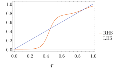
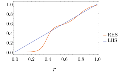
Figure 3: Graphical representation of left- and right-hand side (LHS, RHS) of (41). $D=0.1$, $k_{1}/N=1/2$, $k_{2}/N=1/4$, $\gamma_{0}\cdot\tau=1$. Left: $\nu=0.6$, $\sigma\approx 4.57$, leads to three fix-points; two are stable and one is unstable. Right: $\nu=0.37$, $\sigma\approx 5.19$ gives rise to five fix-points; three stable ones and two unstable ones.

The l.h.s. of equation (41) is a straight line and unbounded whereas the r.h.s. grows monotonically and is bounded between values of the interval $[0,1]$. Hence solutions $r^{*}$ are also in this interval. Solutions with one, three or five intersections can be found. Bifurcations between these monostable, bistable of tristable behavior are saddle-node bifurcations or, if these coincide, a pitchfork bifurcation.

If the number of degrees would be increased, the number of steps will also increase in the same manner, giving rise to even higher multistable states.

3.2 Solutions with vanishing noise

It is illustrative to look first in detail at the case of vanishing noise. Then the r.h.s. of equation (41) vanishes $\propto\exp(-1/D)$ as $r\to 0$ and approaches unity for large values of $r$. In between, the r.h.s. makes two jumps with magnitude $\nu k_{1}/\langle k\rangle$ and $(1-\nu)k_{2}/\langle k\rangle$, respectively. These steps are located at $r_{1}=1/(\sigma k_{1})$ and $r_{2}=1/(\sigma k_{2})$. For the r.h.s. to possess one intersection (monostability) with the straight line $r$, we obtain the following conditions by using that $k_{1}>k_{2}$:

$$\frac{1}{\sigma k_{1}}\,>\,\frac{\nu k_{1}}{\nu k_{1}+(1-\nu)k_{2}},\,\qquad\frac{1}{\sigma k_{2}}>1.$$ (51)

For vanishing noise the monostable state is always the ordered one with $r^{*}=0$, i.e. neither of the two populations is excited.. If one of these inequalities is violated, the mean-field dynamics exhibit bistability. Given that the first one does not hold, besides the ordered solution with $r^{*}=0$, a second stable inhomogeneous state appears. The higher degree population is in the excited state and the lower degree population remains in the non-excited one (cf. Fig. 4(b)). In contrast, if the second inequality is violated bistability occurs between the homogeneous non-excited states and the homogeneous excited ones (cf. Fig. 4(a)). Finally, if both inequalities do not hold, the solution has five intersections according to a tristable solution between the two homogeneous situations and the one non-homogeneous one (cf. Fig. 4(c)).

3.3 Solutions with finite noise and simulations

Examples of the qualitative behavior of the steady states for various noise levels $D$ are presented in Figs. 4(a)-4(c). The graphs have been obtained by numerical solution of (41) and (40). The main difference of these graphs is the ratio $\alpha=k_{1}/k_{2}$. In Fig. 4(a), $\alpha$ equals $3/2$ and for high noise the disordered state with mean-field $r^{*}=1/2$ is stable. The latter bifurcates for lower noise to the known bistability of ordered states Kouvaris2010 which approach $(0,0)$, $(1,1)$ as $D\to 0$. These have been written in terms of the state vector $\mathcal{P}_{1}(t)=(P(1,t|k_{1}),P(1,t|k_{2}))^{\mathrm{T}}$. With respect to the network these solutions are homogeneous states since both populations of the network are ordered in the same states.

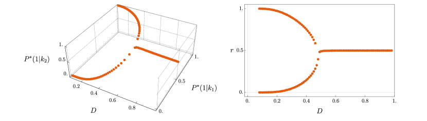
(a)

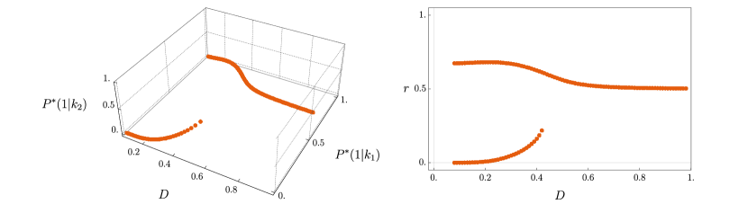
(b)

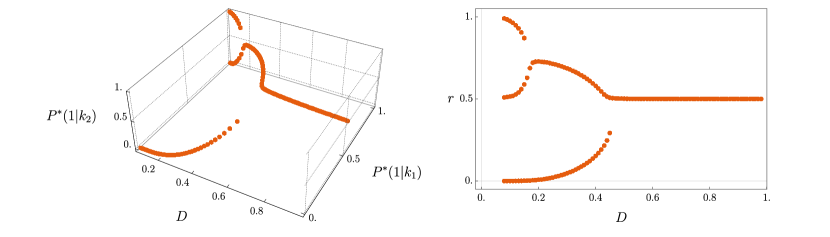
(c)

Figure 4: Stable branches of (37) for $\sigma_{\rm eff}=2$, $\gamma_{0}\cdot\tau=1$, $\nu=0.34$, $k_{1}/N=\frac{1}{2}$ and varying $k_{2}/N$.
4(a)) $k_{2}/N=\frac{1}{3}$: The typical bifurcation into two homogeneous states. This is also observed in networks with all-to-all topology.
4(b)) $k_{2}/N=\frac{1}{8}$: This bifurcation is similar to Fig. 4(a) but the lower degree population cannot be in the excited state anymore.
4(c)) $k_{2}/N=\frac{1}{4}$: In this bifurcation diagram there is a monostable regime for large $D$, a bistable regime with a total ordered and a partial ordered state for intermediate $D$ and the tristable state with three different ordered states for low $D$.

Figure 4(b) presents the qualitative behavior with a strong mismatch of the degrees of the two populations, namely $\alpha=4$. The graph shows that in this parameter region bistability of the two ordered states occurs for lower noise values. With vanishing $D$-values the states become $(0,0)$ and $(0,1)$. In difference to the previous case, the second solution $(0,1)$ is inhomogeneous with respect to the two populations in the network. In the $(0,1)$ state one population is ordered in state $0$ whereas the other approaches an ordered state with mean activity $1$. It is a result of the strong mismatch $\alpha$ of the degrees and of the asymmetry $\nu$ of the two populations. If, for example, the first smaller population with a higher degree is ordered in the excited state $1$, it is not able to excite the second larger population anymore. The latter remains in the ordered rest state $0$.

Also the coexistence of both scenarios is possible and give rise to a tristable parameter region as presented in Fig. 4(c). Here a moderate value of $\alpha=2$ was selected. Lowering the noise intensity, three different regions are visible. First, for high noise $D>0.5$ the monostable disordered solution exists which is apparent in all figures. Lowering the noise this state becomes bistable between the ordered homogeneous states where both populations are in state $0$ and an inhomogeneous network where the population that is smaller and stronger connected is with high probability in the ordered state $1$ but the larger less connected population is still disordered. This is another type of bistability, this time between an homogeneous ordered state and an inhomogeneous disordered state. Finally, by decreasing the noise intensity $D$ further, the third region is entered and the solutions become tristable between $(0,0)$, $(1,0)$ and $(1,1)$ in case of vanishing noise. Stability of the state $(1,0.5)$ as visible in the intermediate region of Fig. 4(c) is an interesting event, because it means that the population of the network with the higher degree is in an ordered state whereas the population with the lower degree is in a disordered state. Such partly ordered states have also been reported for the Ising model on correlated scale-free networks Zhou2007 . These should not be confused with a chimera state, because the units of the subpopulations are not identical and the value of $r$ does not reflect the synchrony of the phases among the units.

In Fig. 5 the distribution of the different stability regimes for varying degree mismatch $\alpha$ and relative concentration $\nu$ are shown for $D=0.1$. The tristable region forms an island surrounded by the different types of bistability and connected to the monostable shore by a very narrow region. Going around the island in an anti-clockwise manner one starts at the homogeneous ordered configuration which gradually becomes more disordered and inhomogeneous with maximal disorder in the middle of the right hand side. After the turning point it gets ordered again but this time in the inhomogeneous regime.

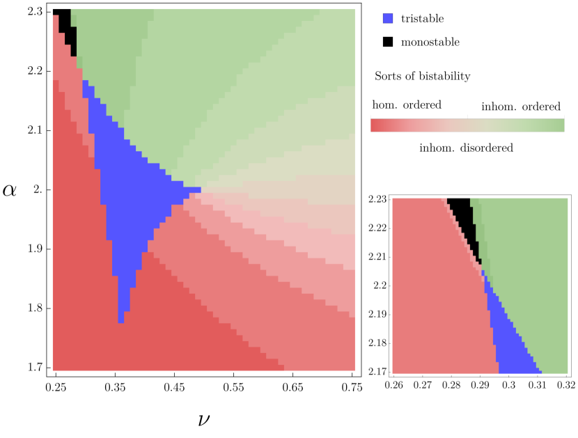
Figure 5: Qualitative behavior of the dynamical regimes in the $\alpha-\nu$ plane for $D=0.1$, $\sigma_{\rm eff}=2$ and $k_{1}/N=1/2$. The graphic beneath the legend is an excerpt of the region between tri- and monostability The two regions will meet in a point which is below resolution.

The presented findings have been confirmed by microscopic simulations of the coupled network, see Eqs. (6) with $w_{0}(t)$ from (5). Numerical investigation of the random binary network is done by solving the Master equations (37) in the Markovian case, namely $w_{1}(t)$ as in (1). As shown in (42) and (40), the equations depend on the first moment of the waiting time distribution rather than the shape of the distribution, although higher moments may play a role for other bifurcations (cf. Appendix A). In addition microscopic simulations of a random binary network with 6000 nodes and full network topology, which corresponds to (10), confirm the made approximations.

Exemplary results are shown in Fig. 6 - 7 which reproduces Fig. 4(c) with two different waiting time distributions. The exponential waiting time distribution which was also used in Fig. 4(c) and a $\delta$-distribution with same mean but no variance.

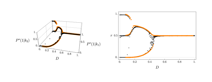
Figure 6: Black stars show the most probable states of the network in a microscopic simulation with $k_{1}=500$, $k_{2}=250$, $N=6000$, $\sigma_{\rm eff}=2$, $\gamma_{0}\cdot\tau=1$, $\nu=0.34$ and $w_{1}(t)$ from (1) after $20\,000$ simulation steps. The orange dots result from the numerical solution of Eq. (37). There are small deviations from Fig. 4(c) which are near the critical points where finite time effects are the strongest. For each $D$-value $11$ equally distributed starting conditions were chosen by preparing the network such that $r\in[0,1]$.

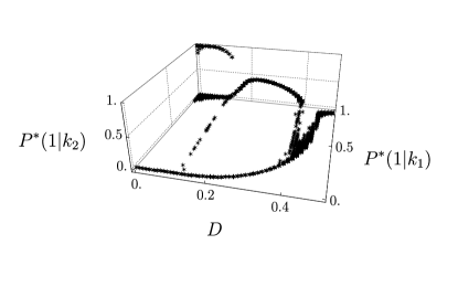
Figure 7: Most probable states of the network in a microscopic simulation in the region $D\in[0,0.5]$ with $w_{1}(t)$ from (2) and other parameters as in Fig. 6. But in this figure for each $D$-value $121$ equally distributed starting conditions were chosen by setting $P(1,0|k_{1})\in[0,1]$ and $P(1,0|k_{2})\in[0,1]$ independently. It shows that the existence of tri- and bistability does not depend on the specific choice of $w_{1}(t)$.

Fig. 8 shows the activity of arbitrary nodes in the two populations in the three different regimes of stable states. The spiking activity of the nodes is presented as symbols versus running time accordingly to the noted degree values $k_{1},k_{2}$ at the r.h.s of the graph.

The firing activity in the two different states is different. As discussed already earlier in Section 2.4, units fire seldom in the rest state, but rapidly in the excited state. This dynamical behavior survives also in the inhomogeneous case. In Fig. 8(a) we present the activity of the units, with an exponential relaxation waiting time distribution. High disorder of the spiking activity in the excited states is the consequence. The CV of the simulated activity is close to $1$, which is the value for an independent Poissonian spike train. Differently, in Fig. 8(b) spiking events from simulations with a $\delta$-distribution are shown. For states where a population $i=1,2$ is in the excited states, i.e. if $P(1|k_{i})\approx 1$, the measured CV possesses values close to zero . This corresponds to a perfectly oscillatory behavior of the units. The period of this spiking coincides with the time $\tau$ the unit stays in the excited state. After this period the unit flips to the rest state. The exponentially distributed time to flip back in the excited state vanishes and also its variance. In consequence, the units behave loike oscillators.

It is important to stress that the constant mean-field value does not correspond to synchronization of the individual units in the excited states, even in case when they practically oscillate. In the rest state the measured CV for both choices of waiting time densities are close to $1$.

4 Conclusion

In this paper, we have investigatedsemi-Markovian stochastic two-state units embedded in a complex network. A theoretical framework has been developed through a heterogeneous mean-field approximation, which is valid for random uncorrelated networks. Our work thus represents an extension of previous studies on globally coupled two-state systems (especially Kouvaris2010 , but also Pinto2014 ; EscaffLind12 ; Dumont2014 ) to two-state systems that have a complex coupling structure.

As an example, we have focused on a random binary network. Thereby we have discovered qualitative changes in the behavior of the steady states. Specifically, structurally new conformations have been found, including tristable and partially ordered states. Additionally the influence of the network on the critical coupling strength has been revealed. We have corroborated all our theoretical results via numerical simulations. We found that the “Markovianity” of the underlying process has no great effect on the positions and the number of steady states and their bifurcations in this simple setting, but still their basins of attraction may be different. Instead the first moment of the waiting time distribution has the greatest impact and higher moments occur only in bifurcations that have at least co-dimension two. It remains for future studies to pursue our analysis explicitly in cases, where more than two different degrees exist. It will be particularly interesting to see how our findings regarding the multistability will generalize.

Networks of stochastic two-state units can be seen as a toy model for magnetic spins, neurons, blinking phenomena or two valued opinions. The occurrence of tristability is also reported in molecular switches Feng2013 ; Lu2013 and in systems of polaritons Cerna2013 ; Paraiso2010 giving hope to perform ternary logical operations in the future. Hence, we expect that our results are relevant for these real-world systems, where the model considered here may serve as an idealized version. The analytic tractability is a strength of our system, but we believe that still many important extensions await consideration, e.g. including network correlations, more sophisticated waiting time distributions or coupling functions.

As underlined previously, the main assumption behind the heterogeneous mean-field approximation is the lack of degree correlations. Random binary networks tend to be disassortative, i.e. nodes with different degrees are preferentially connected as discussed in Sonnenschein2013 . However, for the network examples considered here and for the chosen parameters, these degree correlations become negligible. Therefore, the key assumption is not violated in our study which gave the reason for our analysis. Extending our theory towards correlated networks remains a challenging open problem.

(a)

(b)

Figure 8: Activity of a randomly picked node of each degree of the networks simulated in Figs. 6 - 7 at $D=0.1$ in the three different steady states. Homogeneously activated $(1,1)$, homogeneously at rest $(0,0)$ and inhomogeneously ordered $(1,0)$.
8(a)) Network with exponential $w_{1}$ corresponding to Fig. 6.
8(b)) Network with $\delta$-distributed $w_{1}$ corresponding to Fig. 7.

Author contribution statement
All authors took part in drafting and revising of the manuscript as well as analysis and interpretation of the data. SC carried out simulations and prepared the graphics.

Appendix A Derivation of the characteristic equation

To study the stability of steady states by a characteristic equation, we introduce the vector $\mathcal{P}_{1}(\lambda)$ which is the Laplace transform of the time dependent deviations $\delta\mathcal{P}_{1}(t)=\mathcal{P}_{1}(t)-\mathcal{P}_{1}^{*}$ at a steady state. Then, the linearized version of (37) reads in Laplace space

$$\lambda\mathcal{P}_{1}(\lambda)-\mathcal{P}_{1}(t=0) =\mathsf{J}(\lambda)\mathcal{P}_{1}(\lambda),$$ (52)

with the Jacobian $\mathsf{J}(\lambda)$. Its formal solution is

$$\mathcal{P}_{1}(\lambda) =(\lambda\mathbb{1}-\mathsf{J}(\lambda))^{-1}\mathcal{P}_{1}(t=0)$$

$$=\mathsf{M}^{-1}\mathcal{P}_{1}(t=0).$$ (53)

The final value theorem can be used to calculate the steady states of this system

$$\mathcal{P}_{1}^{*} =\lim_{t\rightarrow\infty}\mathcal{P}_{1}(t)=\lim_{\lambda\rightarrow 0}\lambda\mathcal{P}_{1}(\lambda)$$

$$=\lim_{\lambda\rightarrow 0}\lambda\mathsf{M}^{-1}\mathcal{P}_{1}(t=0)$$

$$=\lim_{\lambda\rightarrow 0}\frac{\lambda}{\det(\mathsf{M})}\text{adj}(\mathsf{M})\mathcal{P}_{1}(t=0),$$ (54)

with

$$\det(\mathsf{M})=\lambda^{2}-\lambda(1-w_{1}(\lambda))\left(\sum_{k}\frac{1}{1+\gamma^{*}_{k}\langle t\rangle}\left(\frac{\partial\gamma^{*}_{k}}{\partial P^{*}_{1,k}}-\gamma^{*}_{k}\right)\right)+$$

$$+(1-w_{1}(\lambda))^{2}\bigg{(}\gamma_{k_{1}}^{*}\gamma_{k_{2}}^{*}-\gamma_{k_{1}}^{*}\frac{1}{1+\gamma_{k_{2}}^{*}\langle t\rangle}\frac{\partial\gamma_{k_{2}}^{*}}{\partial P^{*}(1|k_{2})^{*}}-\gamma_{k_{2}}^{*}\frac{1}{1+\gamma_{k_{1}}^{*}\langle t\rangle}\frac{\partial\gamma_{k_{1}}^{*}}{\partial P^{*}(1|k_{1})^{*}}\bigg{)}$$ (55)

and

$$\text{adj}(\mathsf{M}) =\begin{pmatrix}m_{22}&-m_{12}\\ -m_{21}&m_{11}\\ \end{pmatrix},$$ (56)

$$m_{11} =(1-w_{1}(\lambda))\left(\frac{1}{1+\gamma^{*}_{k_{1}}\langle t\rangle}\frac{\partial\gamma^{*}_{k_{1}}}{\partial P^{*}(1|k_{1})}-\gamma^{*}_{k_{1}}\right)-\lambda,$$

$$m_{12} =(1-w_{1}(\lambda))\frac{1}{1+\gamma^{*}_{k_{1}}\langle t\rangle}\frac{\partial\gamma^{*}_{k_{1}}}{\partial P^{*}(1|k_{2})},$$

$$m_{21} =(1-w_{1}(\lambda))\frac{1}{1+\gamma^{*}_{k_{2}}\langle t\rangle}\frac{\partial\gamma^{*}_{k_{2}}}{\partial P^{*}(1|k_{1})},$$

$$m_{22} =(1-w_{1}(\lambda))\left(\frac{1}{1+\gamma^{*}_{k_{2}}\langle t\rangle}\frac{\partial\gamma^{*}_{k_{2}}}{\partial P^{*}(1|k_{2})}-\gamma^{*}_{k_{2}}\right)-\lambda.$$

The final value theorem states that the limit $\lim_{\lambda\rightarrow 0}\lambda\mathcal{P}_{1}(\lambda)$ is unique if and only if the denominator of $\mathcal{P}_{1}(\lambda)$ has roots with negative real parts and not more than one pole at the origin. Thus indicating bifurcations when one (or several) roots of $\det(\mathsf{M})$ cross the imaginary axis. Therefore $\det(\mathsf{M})=0$ is called the characteristic equation.

The fact that $w_{1}(\lambda)$ is the moment generating function of $w_{1}(t)$ means that $w_{1}(\lambda)=\sum_{k=0}^{\infty}\frac{\langle t^{k}\rangle}{k!}\lambda^{k}$ where $\langle t^{k}\rangle$ is the $k$-th moment of $w_{1}(t)$. Two typical examples are the pairs

$$w_{1}(t)=\delta(t-t_{w}) \longleftrightarrow w_{1}(\lambda)=e^{-\lambda t_{w}}$$ (57)

$$w_{1}(t)=\gamma\,e^{-\gamma\,t} \longleftrightarrow w_{1}(\lambda)=\frac{1}{1+\lambda/\gamma}.$$ (58)

Since $\langle t^{0}\rangle=1$, the term $(1-w_{1}(\lambda))=\sum_{k=1}^{\infty}\frac{\langle t^{k}\rangle}{k!}\lambda^{k}$ and thus $\text{adj}(\mathsf{M})$ is of first order in $\lambda$. Given this information it is clear that $\mathcal{P}_{1}(\lambda)$ has only one pole of order one at the origin.

Appendix B Alternative derivation of (42) using the characteristic equation

To look for saddle-node bifurcations the lowest terms in $\lambda$ of equation (55) will be collected. Identifying $\langle t\rangle=\tau$ results in

$$0= 1-\tau\left(\sum_{k}\left(\frac{1}{1+\gamma^{*}_{k}\tau}\,\frac{\partial\gamma^{*}_{k}}{\partial P^{*}(1|k)}-\gamma^{*}_{k}\right)\right)+$$

$$\tau^{2}\bigg{(}\gamma_{k_{1}}^{*}\gamma_{k_{2}}^{*}-\gamma_{k_{1}}^{*}\frac{1}{1+\gamma_{k_{2}}^{*}\tau}\,\frac{\partial\gamma_{k_{2}}^{*}}{\partial P^{*}(1|k_{2})}-\gamma_{k_{2}}^{*}\frac{1}{1+\gamma_{k_{1}}^{*}\tau}\,\frac{\partial\gamma_{k_{1}}^{*}}{\partial P^{*}(1|k_{1})}\bigg{)}$$

giving

$$\frac{1}{\tau}=\frac{1}{(1+\gamma_{k_{1}}^{*}\tau)^{2}}\,\frac{\partial\gamma_{k_{1}}^{*}}{\partial P^{*}(1|k_{1})}\,+\,\frac{1}{(1+\gamma_{k_{2}}^{*}\tau)^{2}}\,\frac{\partial\gamma_{k_{2}}^{*}}{\partial P^{*}(1|k_{2})}$$ (59)

as the condition for a saddle-node bifurcation. Application of the chain rule in the derivatives, i.e. $\partial\gamma/\partial P=\partial\gamma/\partial r\,\partial r/\partial P$ finally yields

$$\frac{1}{\tau} =\frac{k_{1}\nu}{\langle k\rangle}\frac{1}{(1+\gamma_{k_{1}}^{*}\tau)^{2}}\frac{\partial\gamma_{k_{1}}^{*}}{\partial r^{*}}+\frac{k_{2}(1-\nu)}{\langle k\rangle}\frac{1}{(1+\gamma_{k_{2}}^{*}\tau)^{2}}\frac{\partial\gamma_{k_{2}}^{*}}{\partial r^{*}}.$$ (60)

This is indeed the same equation as (42). This derivation has the positive side effect that with the aid of the characteristic equation all other bifurcation scenarios can be investigated as well.

References

- (1) Frantsuzov P A, Volkán-Kacsó S and Jankó B 2009 Phys. Rev. Lett. 103 207402
- (2) Lindner B, García-Ojalvo J, Neiman A and Schimansky-Geier L 2004 Effects of noise in excitable systems
- (3) Huber D and Tsimring L S 2005 Phys. Rev. E. Stat. Nonlin. Soft Matter Phys. 71 36150
- (4) Pikovsky A and Tsimring L S 2001 Phys. Rev. Lett. 87 250602
- (5) Chen H and Shen C 2015 Phys. A Stat. Mech. its Appl. 424 97–104
- (6) Dumont G, Northoff G and Longtin A 2014 Phys. Rev. E 90 12702
- (7) Prager T, Falcke M, Schimansky-Geier L and Zaks M A 2007 Phys. Rev. E 76 11118
- (8) Colaiori F, Castellano C, Cuskley C F, Loreto V, Pugliese M and Tria F 2015 Phys. Rev. E 91 12808
- (9) Wood K, den Broeck C, Kawai R and Lindenberg K 2006 Phys. Rev. Lett. 96 145701
- (10) Wood K, den Broeck C, Kawai R and Lindenberg K 2007 Phys. Rev. E 76 41132
- (11) Wood K, den Broeck C, Kawai R and Lindenberg K 2006 Phys. Rev. E 74 31113
- (12) Prager T, Naundorf B and Schimansky-Geier L 2003 Coupled three-state oscillators Phys. A Stat. Mech. its Appl. vol 325 pp 176–185
- (13) Escaff D, Harbola U and Lindenberg K 2012 Phys. Rev. E 86 11131
- (14) Kouvaris N, Müller F and Schimansky-Geier L 2010 Phys. Rev. E 82 61124
- (15) Prager T, Lerch H P, Schimansky-Geier L and Schöll E 2007 J. Phys. A Math. Theor. 40 11045
- (16) Leonhardt H, Zaks M A, Falcke M and Schimansky-Geier L 2008 J. Biol. Phys. 34 521–538
- (17) Pinto I L D, Escaff D, Harbola U, Rosas A and Lindenberg K 2014 Phys. Rev. E 89 52143
- (18) Trimper S and Zabrocki K 2004 Memory in diffusive systems
- (19) Cox D R 1962 Renewal Theory Methuen’s monographs on applied probability and statistics (London: Methuen)
- (20) Barrat A, Barthelemy M, Satorras R P and Vespignani A 2004 Proc. Natl. Acad. Sci. U. S. A. 101 3747–3752
- (21) Jiang B 2007 Phys. A 384 647–655
- (22) Mukherjee G, Sen P, Dasgupta S, Chatterjee A, Sreeram P A and Manna S S 2003 Phys. Rev. E. Stat. Nonlin. Soft Matter Phys. 67 36106
- (23) Runions A, Fuhrer M, Lane B, Federl P and Lagan A G R 2005 ACM Trans. Graph. 24 702–711
- (24) Ichinomiya T 2004 Phys. Rev. E - Stat. Nonlinear, Soft Matter Phys. 70
- (25) Sonnenschein B and Schimansky-Geier L 2012 Phys. Rev. E - Stat. Nonlinear, Soft Matter Phys. 85
- (26) Carro A, Toral R and San Miguel M 2016 Sci. Rep. 6 24775
- (27) Rice S 1954 Mathematical analysis of random noise (Dover)
- (28) Hänggi P, Talkner P and Borkovec M 1990 Rev. Mod. Phys. 62 251–341
- (29) Kromer J A, Lindner B and Schimansky-Geier L 2014 Phys. Rev. E - Stat. Nonlinear, Soft Matter Phys. 89
- (30) Lambiotte R 2007 EPL (Europhysics Lett. 78 68002
- (31) Sonnenschein B, Zaks M A, Neiman A B and Schimansky-Geier L 2013 Eur. Phys. J. Spec. Top. 222 2517–2529
- (32) Kouvaris N E 2011 Study of synchronization in discrete biological systems Ph.D. thesis Aristotle university of Thessaloniki, Department of Mathematical, Physical and Computational Sciences
- (33) Restrepo J G, Ott E and Hunt B R 2005 Phys. Rev. E - Stat. Nonlinear, Soft Matter Phys. 71
- (34) Arenas A, Díaz-Guilera A, Kurths J, Moreno Y and Zhou C 2008 Phys. Rep. 469 93–153
- (35) Boccaletti S, Latora V, Moreno Y, Chavez M and Hwang D U 2006 Phys. Rep. 424 175–308
- (36) Newman M E J 2003 SIAM Rev. 45 167–256
- (37) Dorogovtsev S N, Goltsev A V and Mendes J F F 2002 Phys. Rev. E 66 16104
- (38) Zhou H and Lipowsky R 2007 J. Stat. Mech. Theory Exp. 2007 P01009–P01009
- (39) Feng X, Mathoniere C, Jeon I R, Rouzieres M, Ozarowski A, Mathonière C, Rouzières M, Aubrey M, Gonzalez M, Clérac R and Long J 2013 J. Am. Chem. Soc. 135 15880–15884
- (40) Lu M, Jolly M, Gomoto R, Huang B, Onuchic J and Jacob E B 2013 J. Phys. Chem. B 117 13164–13174
- (41) Cerna R, Leger Y, Paraiso T K, Wouters M, Genoud F M, Léger Y, Paraïso T K, Oberli M T P and Deveaud B 2013 Nat. Commun. 4 2008
- (42) Paraiso T K, Wouters M, Leger Y, Genoud F M, Pledran B D, Paraïso T K, Léger Y and Plédran B D 2010 Nat. Mater. 9 655–660