Junction of three off-critical quantum Ising chains and two-channel Kondo effect in a superconductor

Abstract

We show that a junction of three off-critical quantum Ising chains can be regarded as a quantum spin chain realization of the two-channel spin-1/2 overscreened Kondo effect with two superconducting leads. We prove that, as long as the Kondo temperature is larger than the superconducting gap, the equivalent Kondo model flows towards the 2 channel Kondo fixed point. We argue that our system provides the first controlled realization of 2 channel Kondo effect with superconducting leads. Besides its theoretical interest, this result is of importance for potential applications to a number of contexts, including the analysis of the quantum entanglement properties of a Kondo system.

1 Introduction

The Kondo effect Hewson (1993) and the superconductivity Tinkham (2004) are among the most remarkable effects of many-body correlations in condensed matter systems. Specifically, in the former case itinerant electrons conspire to screen a localized magnetic impurity in a conducting media to an isolated spin singlet; in the latter case, electrons pair in two-particle Copper pairs, and eventually condense in a collective ordered state, in which single-particle excitations are fully gapped, with the dependence of the gap on the momentum determined by the specific superconducting state which is created. Remakably, the simultaneous presence of the two effects gives rise to an interesting competition: indeed, it is well-known that Kondo effect is strictly related to low-energy singularities in the single-fermion scattering amplitude of the magnetic impurities, close to the Fermi surface. This clearly conflicts with the presence of an energy gap in the single-fermion spectrum in the superconducting phase, which makes the density of states in the vicinity of the Fermi level equal to 0. Nevertheless, despite the gap, Kondo effect is not necessarily suppressed by the onset of superconductivity. This is due to the well-known result that the fermions effectively screening the impurity are the ones at energies (measured with respect to the Fermi level) ranging from the half-bandwidth all the way down to $k_{B}T_{K}$, with $T_{K}$ being the Kondo temperature and $k_{B}$ the Boltzmann constant Anderson (1970). Therefore, Kondo effect is expected to persist even in a superconducting medium with gap $\Delta$, provided $k_{B}T_{K}\gg\Delta$, which makes the gap itself immaterial for the screening of the magnetic impurity Buitelaar et al. (2002).

In the last two decades, the enormous progress in the fabrication techniques of nanostructures made it possible to realize Kondo effect in a controlled way in e.g. quantum dots at Coulomb blockade Cronenwett et al. (1998); Goldhaber-Gordon et al. (1998) or in single magnetic impurities procolo in contact with metallic leads. More generally, Kondo effect in low-dimensional systems has been explored Dell’Anna (2010), especially in view of its relation to remarkable many-body collective effects avishai_book, such as, for instance the electronic shake-up after a single-electron emission ort_kondo; sindona_1. This motivated further proposals for studying the coexistence/competition between Kondo effect and superconductivity in a quantum dot coupled to superconducting leads, also in a Josephson-junction arrangement (dot connected to two superconducting leads at zero voltage bias and fixed phase difference), which should be able to evidence the crossover between $\pi$-junction (no Kondo effect) and 0-junction (onset of the Kondo effect) Avishai et al. (2001); Choi et al. (2001, 2004); Campagnano et al. (2004). On the experimental side, a remarkable scaling law of the dc-conductance, which results to be a universal function of $\Delta/(k_{B}T_{K})$, has been observed in a single quantum dot contacted laterally to a superconducting reservoir Buizert et al. (2007). While there is still some debate about nonuniversal features, it is basically estabilished that the onset of Kondo effect is effective whenever $K_{B}T_{K}/\Delta\gg 1$ and that the fixed point as $T\to 0$ should correspond to the perfectly screened Nozières fermi liquid Hewson (1993). Other issues which have been studied using quantum dots connected to superconductors are, for instance, the interplay between Kondo effect and Andreev reflection in dots coupled to one normal and one superconducting lead Oguri et al. (2013), or in a dot coupled to topological superconducting leads Lee et al. (2013).

Recently, novel possible realizations of Kondo effect have been proposed at junctions of interacting quantum wires and topological superconductors Béri and Cooper (2012); Altland et al. (2014a); Eriksson et al. (2014); Altland et al. (2014b), in an SNS-junction made with topological superconductors (where it should be detected by looking at the scaling of the current with the system size) GiuAf2; GiuAf3, or in junctions of quantum spin chains Crampè and Trombettoni (2013); Tsvelik (2013); Giuliano and Sodano (2013); Giuliano et al. (2016). In particular, the quantum spin chain realization of the Kondo effect presents a number of theoretically interesting features, such as the possibility of realizing in a ”natural” way the symmetry between channels in the many-channel version of the effect Tsvelik (2013) or, on the theoretical side, the exact integrability of some specific models Tsvelik (2014); Buccheri et al. (2015). On the applicative side, it appears particularly intriguing, due to the possibility of realizing in a controlled way devices behaving as spin chains and/or as junctions of spin chains by means, for instance, of pertinently engineered superconducting quantum wires Giuliano and Sodano (2007), or of quantum Josephson junction networks Giuliano and Sodano (2009, 2010); Cirillo et al. (2011).

In a junction of quantum spin chains the magnetic impurity is determined by the coupling between the chains. Formally, this is evidenced by extending to the junction the Jordan-Wigner transformation Jordan and Wigner (1928), by means of which one realizes quantum spin-1/2 operators in terms of lattice spinless fermion operators (and vice versa). When applied to a junction of more than two chains, the Jordan-Wigner tranformation requires introducing ancillary fermionic degrees of freedom, to preserve the correct commutation relations between corresponding operators. At a three-chain junction, this determines an effective spin-1/2 magnetic impurity which is topological, due to the nonlocal character of the ancillary degrees of freedom Crampè and Trombettoni (2013). The Jordan-Wigner fermion can, therefore, act to realize Kondo effect by screening this effective magnetic impurity. Along this correspondence, in order to recover a gapless single-fermion spectrum, an important requisite is that the chains forming the junction are all tuned at a quantum critical point, either corresponding to the paramagnetic-ferromagnetic phase transition in the quantum-Ising chains Tsvelik (2013); Giuliano and Sodano (2013) or in the XY quantum spin chains Giuliano et al. (2016), or belonging to a critical line of gapless points, such as in the junction of quantum XX spin chains Crampè and Trombettoni (2013).

In this paper we rather focus onto the Kondo effect at a junction of three off-critical (on either the paramagnetic, or the ferromagnetic side) quantum Ising chains, with a nonzero gap in the single-fermion spectrum. Specifically, by going through a rigorous mapping between the off-critical junction of Ising chains and the model for a spin-1/2 magnetic impurity interacting with two superconducting baths, we prove that our system can be regarded as a model for two-channel Kondo effect with superconducting leads.

A first important feature of the system we consider is that it hosts a remarkable realization of overscreened, spin-1/2 two-channel Kondo effect with superconducting electronic baths which, so far, has never emerged in realistic devices based on e.g. quantum dots with superconducting leads. Moreover, our system naturally presents a symmetry between channel, which is typically hard to recover in ”standard” condensed matter-based many-channel Kondo systems Tsvelik (2013); Coleman et al. (1995). Finally, the very fact that our system is based on a junction of spin chains makes it possible to use it for potentially countless numerically- and analitically-based applications, such as, for instance, probing the effects of superconductivity on the entanglement structure of the system Alkurtass et al. (2016) and, more generally, verifying how the Kondo interaction affects the entanglement of the spin chains close to their ”bulk” quantum critical point Amico et al. (2008); Giuliano et al. (2010).

The paper is organized as follows:

• In section 2, we introduce the model Hamiltonian for the junction of three quantum spin chains and map it onto a pertinent fermionic Hamiltonian by employing an adapted version Crampè and Trombettoni (2013) of the Jordan-Wigner transformation;

• In section 3, we rigorously trace out the mapping between the Jordan-Wigner fermionic representation of the junction Hamiltonian and a model for a quantum spin-1/2 impurity interacting with two superconducting baths (”channels”);

• In section 4, we analyze the onset of Kondo regime by means of a pertinently adapted version Giuliano et al. (2016) of poor man’s renormalization group approach to Kondo problem Anderson (1970), finding the necessary conditions to which the Kondo coupling and the single-fermion energy gap must obey, in order to actually recover the Kondo effect;

• In section 5, we discuss whether, and how, Majorana-fermion-like excitations arising at the endpoints of the chains in the magnetically ordered phase affect the Kondo effect, proving that their are basically irrelevant for what concerns Kondo physics;

• In section 6, we describe the strongly coupled Kondo fixed point of the system using a variational approach Campagnano et al. (2004); Giuliano and Tagliacozzo (2004), adapted to the specific case of gapped leads. We conclude that the gap does not substantially affect the structure of the Kondo fixed point, provided the conditions for the onset of Kondo regime are met;

• In section 7, we provide our main conclusions, together with a discussion of possible further developments of our work;

• In appendix A, we present mathematical details about the exact solution of a quantum Ising chain with open boundary conditions in terms of Jordan-Wigner fermions.

2 The model Hamiltonian for the junction

The possibility of realizing two-channel Kondo (2CK) effect at a junction of three critical ferromagnetic quantum Ising chains (QIC)s was originally put forward by Tsvelik Tsvelik (2013) who, later on, also proved the exact solvability of the model, taken in the continuum limit Tsvelik (2014). Here, we consider the generic situation of a junction of three, non (necessarily) critical QICs. Following Tsvelik’s construction, we focus onto a junction of three equal chains, each one consisting of $\ell$ sites. The three (disconnected) chains are described by the model Hamiltonian

$$H_{\rm Chain}=\sum_{\lambda=1}^{3}\>\Biggl{\{}-J\sum_{j=1}^{\ell-1}S_{j+1,\lambda}^{x}S_{j,\lambda}^{x}+h\sum_{j=1}^{\ell}S_{j,\lambda}^{z}\Biggr{\}}\>\>\>\>.$$ (1)

In Eq.(1), $S_{j,\lambda}^{x}$ and $S_{j,\lambda}^{z}$ are quantum, spin-1/2 operators acting on site-$j$ of chain-$\lambda$, $J$ ($>0$) is the ferromagnetic exchange strength between spins on nearest neighboring sites, $h$ is the applied magnetic field in the $z$-direction. With the normalization we chose in Eq.(1), the chains become quantum critical at $J=\pm h/2$ Sachdev (2011). The junction is constructed by connecting the three spins at the endpoints of the three chains by means of a ferromagnetic coupling $J_{\Delta}<J$. The corresponding boundary Hamiltonian is therefore given by

$$H_{\Delta}=-J_{\Delta}\sum_{\lambda=1}^{3}S_{1,\lambda+1}^{x}S_{1,\lambda}^{x}\>\>\>\>,$$ (2)

with periodicity in the index $\lambda$ understood, that is, $S_{1,\lambda+3}^{x}=S_{1,\lambda}^{x}$. The whole system is described by the model Hamiltonian $H=H_{\rm Chains}+H_{\Delta}$. The mapping of the spin-chain junction onto a fermionic Kondo-like Hamiltonian is based onto a generalization of the Jordan-Wigner (JW) fermionization procedure for a single chain with open boundary conditions, which we review in appendix A. Specifically, in order to preserve the correct (anti)commutation relations between operators acting on different chains, one has to introduce a set of Jordan-Wigner spinless lattice fermions per each chain, $\{a_{j,\lambda},a_{j,\lambda}^{\dagger}\}$, in analogy to what is tipically done for a single chain (see appendix A for details) and, in addition, three real-fermionic Klein factors (KF)’s $\sigma^{\lambda}$, one per each chain Crampè and Trombettoni (2013). By definition, each $\sigma^{\lambda}$ anticommutes with all the $a_{j,\lambda^{\prime}},a_{j,\lambda^{\prime}}^{\dagger}$. On introducing the KFs, the JW transformations in Eq.(46) of appendix A are generalized to Crampè and Trombettoni (2013); Tsvelik (2013); Giuliano et al. (2016)

$$S_{j,\lambda}^{+} = ia_{j,\lambda}^{\dagger}\>e^{i\pi\sum_{r=1}^{j-1}a_{r,\lambda}^{\dagger}a_{r,\lambda}}\sigma^{\lambda}$$

$$S_{j,\lambda}^{-} = ia_{j,\lambda}\>e^{i\pi\sum_{r=1}^{j-1}a_{r,\lambda}^{\dagger}a_{r,\lambda}}\sigma^{\lambda}$$

$$S_{j,\lambda}^{z} = a_{j,\lambda}^{\dagger}a_{j,\lambda}-\frac{1}{2}\>\>\>\>.$$ (3)

Due to the identity $(\sigma^{\lambda})^{2}=1$, it is easy to check that, when inserting Eqs.(3) into Eq.(1), the KFs fully disappear from $H_{\rm Chain}$ and that, accordingly, one obtains

$$H_{\rm Chain} = \sum_{\lambda=1}^{3}\Biggl{\{}-\frac{J}{4}\sum_{j=1}^{\ell-1}\>\{a_{j,\lambda}^{\dagger}a_{j+1,\lambda}+a_{j+1,\lambda}^{\dagger}a_{j,\lambda}\}$$ (4)

$$- \frac{J}{4}\sum_{j=1}^{\ell-1}\>\{a_{j,\lambda}a_{j+1,\lambda}+a_{j+1,\lambda}^{\dagger}a_{j,\lambda}^{\dagger}\}+h\sum_{j=1}^{\ell}a_{j,\lambda}^{\dagger}a_{j,\lambda}\Biggr{\}}\>\>\>\>.$$

At variance, the KFs do explicitly appear in $H_{\Delta}$, which takes the form

$$H_{\Delta}=\sum_{\lambda=1}^{3}{\cal T}^{\lambda}\Sigma_{1}^{\lambda}\>\>\>\>,$$ (5)

with

$$\Sigma_{j}^{\lambda}=-\frac{i}{2}\>\sum_{\lambda^{\prime},\lambda^{{}^{\prime\prime}}}\>\epsilon^{\lambda,\lambda^{\prime},\lambda^{{}^{\prime\prime}}}\>[a_{j,\lambda^{\prime}}^{\dagger}+a_{j,\lambda^{\prime}}][a_{j,\lambda^{{}^{\prime\prime}}}^{\dagger}+a_{j,\lambda^{{}^{\prime\prime}}}]\>\>\>\>,$$ (6)

and the effective spin-1/2 operator $\vec{\cal T}$ being given by

$${\cal T}^{\lambda}=-\frac{i}{2}\>\sum_{\lambda^{\prime},\lambda^{{}^{\prime\prime}}}\>\epsilon^{\lambda,\lambda^{\prime},\lambda^{{}^{\prime\prime}}}\sigma^{\lambda^{\prime}}\sigma^{\lambda^{{}^{\prime\prime}}}\>\>\>\>.$$ (7)

The operator $\vec{\cal T}$ typically arises when employing the generalized JW fermionization procedure at a junction of three quantum spin chains Crampè and Trombettoni (2013); Tsvelik (2013); Giuliano et al. (2016): it is regarded as a topological spin-1/2 operator because of its nonlocal character in both the chain and the site index, despite the fact that it only appears in the boundary Hamiltonian $H_{\Delta}$, which is ”concentrated” at the common boundary (the junction) at $j=1$ Béri and Cooper (2012); Béri (2013). As highlighted in appendix A, $H_{\rm Chain}$ in Eq.(4) can be regarded as the sum of three Kitaev Hamiltonians for a one-dimensional p-wave superconductor: on this analogy we will ground most of the following discussion on our system.

3 Mapping onto the two-channel Kondo model with superconducting leads

We are now going to rigorously show that a junction of three off-critical quantum Ising chains can be mapped onto the Kondo problem for a spin-1/2 impurity in contact with two superconducting baths (”channels”). Specifically, we adapt to our problem the mapping procedure derived and discussed in Ref.Coleman et al. (1995) in the case of normal leads. The key step is to go through the expression of the boundary Hamiltonian in terms of Bogoliubov operators for a quasiparticle with energy $\epsilon$, $\{\Gamma_{\epsilon}\}$. This can be done by inverting Eqs.(49) of appendix A and by considering that, in a spinless superconductor, one has the particle-hole correspondence encoded in the relation $\Gamma_{-\epsilon}=\Gamma_{\epsilon}^{\dagger}$, which can be explicitly checked from Eqs.(49,53,55) of appendix A. Looking at the explicit formulas for the quasiparticle wavefunctions, Eqs.(53,55), one therefore obtains

$$a_{1}^{\dagger}+a_{1}=\sum_{\epsilon\neq 0}\left[\frac{\sin(k+\varphi_{k})}{\sqrt{\ell+1}}\right][\Gamma_{\epsilon}+\Gamma_{\epsilon}^{\dagger}]+\left[\frac{\sqrt{2J^{2}-8h^{2}}}{J}\right]\Gamma_{0,L}\>\>\>\>.$$ (8)

$\Gamma_{0,L}$ is the mode operator for the Majorana mode localized at the left-hand endpoint of the chain: the corresponding term in the mode expansion of Eq.(8) only appears in the topological phase of the Kitaev-like Hamiltonian, corresponding to the magnetically ordered phase of the quantum Ising chain. As we discuss in the following, whether a term $\propto\Gamma_{0,L}$ is present in the mode expansion of Eq.(8), or not, does not substantially affect the Kondo physics of the system. Thus, in the following of this section we shall just disregard it and accordingly truncate the mode expansion of $a_{1}^{\dagger}+a_{1}$ to the first term at the right-hand side of Eq.(8). As a result, we eventually obtain

$$a_{1}^{\dagger}+a_{1}=\sqrt{\frac{2}{\ell+1}}\>\sum_{\epsilon}\left[\sin(k+\varphi_{k})[\Gamma_{\epsilon_{k}}+\Gamma_{\epsilon_{k}}^{\dagger}]\right]\>\>\>\>.$$ (9)

By means of an appropriate and straightforward generalization of Eq.(9), we therefore rewrite $\Sigma_{1}^{\lambda}$ in Eq.(7) as

$$\Sigma_{1}^{\lambda} = -\frac{i}{(\ell+1)}\>\sum_{\lambda^{\prime},\lambda^{{}^{\prime\prime}}}\>\sum_{\epsilon^{\prime},\epsilon^{{}^{\prime\prime}}}\>\epsilon^{\lambda,\lambda^{\prime},\lambda^{{}^{\prime\prime}}}\>\left[\frac{h^{2}\sin(k^{\prime})\sin(k^{{}^{\prime\prime}})}{\epsilon_{k^{\prime}}\epsilon_{k^{{}^{\prime\prime}}}}\right]$$ (10)

$$\times [\Gamma_{\epsilon_{k^{\prime}},\lambda^{\prime}}+\Gamma_{\epsilon_{k^{\prime}},\lambda^{\prime}}^{\dagger}][\Gamma_{\epsilon_{k^{{}^{\prime\prime}}},\lambda^{{}^{\prime\prime}}}+\Gamma_{\epsilon_{k^{{}^{\prime\prime}}},\lambda^{{}^{\prime\prime}}}^{\dagger}]\>\>\>\>.$$

The ”bulk” of the chains is instead described by the simple quadratic Hamiltonian given by

$$H_{\rm Chain}=\sum_{\lambda=1}^{3}\>\sum_{\epsilon}\>\epsilon\>\Gamma_{\epsilon,\lambda}^{\dagger}\Gamma_{\epsilon,\lambda}\>\>\>\>.$$ (11)

As we are now going to show, by following the main recipe presented in Ref.Coleman et al. (1995), it is possible to readily recover the total Hamiltonian $H=H_{\rm Chain}+H_{\Delta}$ in terms of an appropriate model Hamiltonian for two superconducting quasiparticle baths undergoing an appropriate Kondo-like interaction with the spin $\vec{\cal T}$ of an isolated spin-1/2 impurity. To do so, let us introduce two sets of quasiparticle annihilation and creation operators, $\{\gamma_{\epsilon,a},\gamma_{\epsilon,a}^{\dagger}\}$, with $a=1,2$, obeying the anticommutation algebra $\{\gamma_{\epsilon,a},\gamma_{\epsilon^{\prime},a^{\prime}}^{\dagger}\}=\delta_{\epsilon,\epsilon^{\prime}}\delta_{a,a^{\prime}}$. Also, we choose the energy levels $\epsilon$ to cohincide with the eigenvalues of the single-chain Hamiltonian in Eq.(48), so that the Hamiltonian for the $\gamma$-modes is given by

$$H_{\gamma}=\sum_{\epsilon}\sum_{a}\epsilon\gamma_{\epsilon,a}^{\dagger}\gamma_{\epsilon,a}\>\>\>\>.$$ (12)

Next. we define real-space lattice fermion operators $\{d_{j,a}\}$ as

$$d_{j,1} = \sum_{\epsilon}\{u_{j}^{\epsilon}\gamma_{\epsilon,1}-v_{j}^{\epsilon}\gamma_{\epsilon,2}^{\dagger}\}$$

$$d_{j,2} = \sum_{\epsilon}\{u_{j}^{\epsilon}\gamma_{\epsilon,2}+v_{j}^{\epsilon}\gamma_{\epsilon,1}^{\dagger}\}\;\;\;\;,$$ (13)

with the wavefunctions $u_{j}^{\epsilon},v_{j}^{\epsilon}$ given in Eqs.(53,55). Now, we notice that, going backwards to a possible lattice Hamiltonian formulation of our construction, we may construct the $\gamma_{\epsilon,a}$-operators as eigenmodes of the superconducting lattice Hamiltonian $H_{\rm Eff}$, defined as

$$H_{\rm Eff}= - \frac{J}{4}\sum_{a=1,2}\sum_{j=1}^{\ell-1}\{d_{j,a}^{\dagger}d_{j+1,a}+d_{j+1,a}^{\dagger}d_{j,a}\}$$ (14)

$$- \frac{J}{4}\sum_{j=1}^{\ell-1}\{d_{j,1}d_{j+1,2}-d_{j,2}d_{j+1,1}+d_{j+1,2}^{\dagger}d_{j,1}^{\dagger}-d_{j+1,1}^{\dagger}d_{j,2}^{\dagger}\}$$

$$+ h\sum_{a=1,2}\sum_{j=1}^{\ell}d_{j,a}^{\dagger}d_{j,a}\>\>\>\>.$$

As proposed in Ref.Coleman et al. (1995), we now use the modes of $H_{\rm Eff}$ two define two independent lattice isospin operators, ${\bf S}_{j}$ and ${\bf T}_{j}$, respectively given by

$${\bf S}_{j}=\frac{1}{2}\>\left[\begin{array}[]{c}d_{j,1}^{\dagger}d_{j,2}+d_{j,2}^{\dagger}d_{j,1}\\ -i(d_{j,1}^{\dagger}d_{j,2}-d_{j,2}^{\dagger}d_{j,1})\\ d_{j,1}^{\dagger}d_{j,1}-d_{j,2}^{\dagger}d_{j,2}\end{array}\right]\>\>\>\>,$$ (15)

and by

$${\bf T}_{j}=\left[\begin{array}[]{c}d_{j,1}^{\dagger}d_{j,2}^{\dagger}+d_{j,2}d_{j,1}\\ -i(d_{j,1}^{\dagger}d_{j,2}^{\dagger}-d_{j,2}d_{j,1})\\ d_{j,1}^{\dagger}d_{j,1}+d_{j,2}^{\dagger}d_{j,2}-1\end{array}\right]\>\>\>\>.$$ (16)

Any component of ${\bf S}_{j}$ commutes with any component of ${\bf T}_{j}$: therefore, the two of them can be regarded as two independent spin-1/2 lattice density operators. Using them as independent channels to screen an isolated spin-1/2 impurity with spin $\vec{\cal T}$, coupled to the site $j=1$ by means of the antiferromagnetic Kondo coupling $J_{K}$, we may write the corresponding boundary Kondo Hamiltonian as

$$H_{K}=J_{K}\sum_{\lambda=1}^{3}\{[S_{1}^{\lambda}+T_{1}^{\lambda}]{\cal T}^{\lambda}\}=$$ (17)

$$- \frac{iJ_{K}}{2}[i(d_{1,1}^{\dagger}-d_{1,1})][d_{1,2}^{\dagger}+d_{1,2}]{\cal T}^{1}+[d_{1,2}^{\dagger}+d_{1,2}][d_{1,1}^{\dagger}+d_{1,1}]{\cal T}^{2}$$

$$+ [d_{1,1}^{\dagger}d_{1,1}][i(d_{1,1}^{\dagger}-d_{1,1})]{\cal T}^{3}\}\>\>\>\>.$$

From Eq.(17) and from the tranformations from the $\gamma$- to the $d$-modes in Eqs.(13), one eventually recovers the Hamiltonian $H_{\Delta}$, once the following identifications are performed

$$\Gamma_{\epsilon,1}+\Gamma_{\epsilon,1}^{\dagger} \leftrightarrow d_{1,1}^{\dagger}+d_{1,1}$$

$$\Gamma_{\epsilon,2}+\Gamma_{\epsilon,2}^{\dagger} \leftrightarrow i(d_{1,1}^{\dagger}-d_{1,1})$$

$$\Gamma_{\epsilon,3}+\Gamma_{\epsilon,3}^{\dagger} \leftrightarrow d_{1,2}^{\dagger}+d_{1,2}\>\>\>\>,$$ (18)

and, of course, $J_{k}\leftrightarrow J_{\Delta}$. The correspondence rules in Eqs.(18) complete the mapping procedure between the lattice two-channel superconducting-Kondo Hamiltonian $H_{\rm Eff}+H_{K}$ and the model Hamiltonian for a junction of three quantum Ising chains. A remarkable feature of our mapping procedure is that it relies on the construction of the spin densities for the two independent channels as in Eqs.(16,17). As extensively discussed in Ref.Coleman et al. (1995), constructing the spin densities in this way implies that, if a site $j$ contains a total spin-1/2 of the ${\bf S}_{j}$-operator, than it must be a singlet of the ${\bf T}_{j}$-operator, with corresponding spin equal to 0, and vice versa. In the ”classical” two-channel Kondo problem, this is crucial a crucial point to build an effective theory for the system at the 2CK-fixed point which, in this regularization scheme, is pushed all the way down to strong coupling, such as in the 1CK-problem Coleman et al. (1995); Giuliano and Tagliacozzo (2004). In the following, we will make use of this properties to get insights of the nature of the fixed point toward which our system is attracted along the Kondo renormalization group trajectory.

4 Perturbative renormalizazion group analysis of the Kondo interaction

In this section, we derive the perturbative renormalization group (RG) equations for the running coupling $J_{\Delta}$. As stated above, for the time being, we disregard the zero-mode Majorana modes in the expansion of $a_{1,\lambda}^{\dagger}+a_{1,\lambda}$: we will come back to a discussion of their effects in the next section. To work out the perturbative renormalization of $J_{\Delta}$, we resort to the imaginary time path-integral formalism, by introducing the Euclidean bulk action for the chains, $S_{\rm Chain}$, given by

$$S_{\rm Chain}=\int\>d\tau\>\left\{\sum_{\lambda=1}^{3}\sum_{j=1}^{\ell}a_{j,\lambda}^{\dagger}(\tau)\partial_{\tau}a_{j,\lambda}(\tau)+H_{\rm Chain}(\tau)\right\}\;\;\;\;,$$ (19)

as well as the boundary action $S_{\Delta}$, which is given by

$$S_{\Delta}=J_{\Delta}\>\int\>d\tau\>\sum_{\lambda=1}^{3}\>{\cal T}^{\lambda}(\tau)\Sigma_{1}^{\lambda}(\tau)\>\>\>\>.$$ (20)

Using $H_{\rm Chain}$ as noninteracting Hamiltonian, in the corresponding interaction representation one may present the partition function for the junction, ${\cal Z}$, as

$${\cal Z}={\cal Z}_{0}\langle{\bf T}_{\tau}\exp[-S_{\Delta}]\rangle\>\>\>\>,$$ (21)

with ${\cal Z}_{0}$ being the partition function for the system at $J_{\Delta}=0$, $S_{\Delta}$ being the boundary action in the interaction representation, and ${\bf T}_{\tau}$ being the imaginary time ordering operator. Following the standard poor man’s recipe to recover the RG equation Anderson (1970); Hewson (1993), we now resort to the frequency domain and explicitly cutoff the integration over frequencies at a scale $D$, so that $S_{\Delta}$ can be rewritten as

$$S_{\Delta}=\int_{-D}^{D}\>\frac{d\Omega}{2\pi}\>\sum_{\lambda=1}^{3}\>{\cal T}^{\lambda}(\Omega)\Sigma_{1}^{\lambda}(-\Omega)\>\>\>\>,$$ (22)

with ${\cal T}^{\lambda}(\Omega)$ and $\Sigma_{1}^{\lambda}(\Omega)$ being the Fourier transform of respectively ${\cal T}^{\lambda}(\tau)$ and $\Sigma_{1}^{\lambda}(\tau)$. To derive the RG equations for the running coupling, we rescale the cutoff from $D$ to $D/\kappa$, with $0<\kappa-1\ll 1$ and, accordingly, we split the integral in Eq.(22) into an integral over $[-D/\kappa,D/\kappa]$ plus integrals over values of $\Omega$ within $[D/\kappa,D]$ and within $[-D,-D/\kappa]$. Leaving aside the two latter integral, as they just provide a correction to the total free energy. We therefore obtain, in analogy to Giuliano et al. (2016)

$$S_{\Delta} \to \int_{-\frac{D}{\kappa}}^{\frac{D}{\kappa}}\>\frac{d\Omega}{2\pi}\>\sum_{\lambda=1}^{3}\>{\cal T}^{\lambda}(\Omega)\Sigma_{1}^{\lambda}(-\Omega)$$ (23)

$$= \frac{1}{\kappa}\int_{-D}^{D}\>\frac{d\Omega}{2\pi}\>\sum_{\lambda=1}^{3}\>{\cal T}^{\lambda}(\frac{\Omega}{\kappa})\Sigma_{1}^{\lambda}(-\frac{\Omega}{\kappa})\;\;\;\;,$$

which, since $S_{\Delta}$ must be scale invariant, implies Giuliano et al. (2016) $\sum_{\lambda=1}^{3}\>{\cal T}^{\lambda}(\frac{\Omega}{\kappa})\Sigma_{1}^{\lambda}(-\frac{\Omega}{\kappa})=\kappa\sum_{\lambda=1}^{3}\>{\cal T}^{\lambda}(\Omega)\Sigma_{1}^{\lambda}(-\Omega)$. Therefore, $J_{\Delta}$ takes no corrections to first order in the boundary coupling. At variance, to second order one finds a nonzero correction, arising from summing over intermediate states with energies within $[D/\kappa,D]$ and within $[-D,-D/\kappa]$. Performing the integration, one eventually obtains that, to leading order in $J_{\Delta}$ (corresponding to one-loop order in the expansion of the action in $S_{\Delta}$), $S_{\Delta}$ is corrected according to $S_{\Delta}\to S_{\Delta}+\delta S_{\Delta}^{(2)}$, with Giuliano et al. (2016)

$$\delta S_{\Delta}^{(2)}=J_{\Delta}^{2}\int_{-D}^{D}\>\sum_{\lambda=1}^{3}\>\frac{d\Omega}{2\pi}\>{\cal T}^{\lambda}(\Omega)\Sigma_{1}^{\lambda}(-\Omega)[\Gamma(D)+\Gamma(-D)]D(1-\kappa^{-1})\>\>\>\>.$$ (24)

The function $\Gamma(\Omega)$ in Eq.(24) is defined to be the Fourier-Matsubara transform of $\Gamma(\tau)=G(\tau)g(\tau)$, with $g(\tau)={\rm sgn}(\tau)$ being the $\sigma$-fermion Green’s function $g(\tau)=\langle{\bf T}_{\tau}[\sigma(\tau)\sigma(0)]\rangle$ and $G(\tau)$ being the imaginary time ordered Green’s function (effectively independent of $\lambda$, due to the equivalence between the three chains)

$$G(\tau)=-\langle{\bf T}_{\tau}\{[a_{1,\lambda}^{\dagger}(\tau)+a_{1,\lambda}(\tau)][a_{1,\lambda}^{\dagger}(0)+a_{1,\lambda}(0)]\}\rangle\>\>\>\>.$$ (25)

From Eqs.(24,25) one may eventually derive the RG equations for the running coupling $J_{\Delta}(D)$ in the form

$$\frac{dJ_{\Delta}(D)}{d\ln\left(\frac{D_{0}}{D}\right)}=J_{\Delta}^{2}(D)\rho(D)\>\>\>\>,$$ (26)

with, in the specific system we are focusing on, $\rho(D)$ being given by

$$\rho(D)=\frac{16}{\pi J^{2}}\>\int_{\Delta_{w}}^{W}\>d\epsilon\>\left[\frac{D^{2}}{(\epsilon^{2}+D^{2})^{2}}\right]\sqrt{(\epsilon^{2}-\Delta_{w}^{2})(W^{2}-\epsilon^{2})}\>\>\>\>.$$ (27)

In Eq.(27), we used $\Delta_{w}$ to denote the single-fermion excitation gap, as discussed in appendix A, while $W=\frac{J}{2}+|h|$ is the energy at the band edge in the single-fermion spectrum and $D_{0}$ is a ${\cal O}(W)$ high-energy reference cutoff. On integrating Eq.(27), one may therefore infer whether the system crosses over towards the Kondo regime, despite the presence of a nonzero gap $\Delta_{w}$ in the spectrum, and, if that is the case, what is the corresponding (Kondo) temperature scale at which the crossover takes place. To analyze the onset of the Kondo regime, we follow the technique highlighted in Dell’Anna (2010). Specifically, we introduce the ($\Delta_{w}$-dependent) ”critical coupling” $J_{\Delta}^{c}(\Delta_{w})$, defined as

$$J_{\Delta}^{c}(\Delta_{w})=\Biggl{\{}\int_{0}^{D_{0}}\>\rho(x)\frac{dx}{x}\Biggr{\}}^{-1}\>\>\>\>.$$ (28)

(Note that, in the definition of $J_{\Delta}^{c}$, we stressed the dependence on the gap $\Delta_{w}$. This is a basic feature of our ”off-critical” model, which makes the main difference between the case we investigate here and the critical limit, extensively discussed in Tsvelik (2013); Giuliano et al. (2016).) Having introduced the critical coupling, the solution to Eq.(26) can be rewritten as

$$J_{\Delta}(D)=\frac{J_{\Delta}(D_{0})J_{\Delta}^{c}(\Delta_{w})}{J_{\Delta}(D_{0})-J_{\Delta}^{c}(\Delta_{w})+J_{\Delta}(D_{0})J_{\Delta}^{c}(\Delta_{w})\>\int_{0}^{D}\rho(x)\frac{dx}{x}}\>\>\>\>.$$ (29)

Within standard poor man’s approach to Kondo problem, the onset of the Kondo regime is signaled by the appearance of a scale $D_{K}$ at which $J_{\Delta}(D)$ diverges. At $D=D_{K}$, therefore, the denominator of the expression at the right-hand side of Eq.(29) must be equal to 0, which is only possible if $J_{\Delta}(D_{0})\geq J_{\Delta}^{c}(\Delta_{w})$. This observation implies that Kondo effect does definitely not take place whenever $J_{\Delta}^{c}(\Delta_{w})/W>1$. At variance, for $J_{\Delta}^{c}(\Delta_{w})/W<1$ the crossover to Kondo regime can take place within an appropriate range of values of $J_{\Delta}(D_{0})$, provided the Kondo crossover scale $D_{K}$, though substantially lower than $W$, is still $>\Delta_{w}$, so to have a nonzero fermion density screening the isolated magnetic impurity at the scale $D_{K}$ Avishai et al. (2001); Choi et al. (2001); Campagnano et al. (2004); Choi et al. (2004). In Fig.1, we plot $J_{\Delta}^{c}(\Delta_{w})/W$ as a function of $\Delta_{w}$. The dashed horizontal line marks the set of points corresponding to $J_{\Delta}^{c}/W=1$. Consistently with what we discuss before, we expect that Kondo regime is fully suppressed by the gap in the single-fermion spectrum throughout all the region with $J_{\Delta}^{c}/W>1$, that is, for $\Delta_{w}>\Delta_{w}^{*}\approx 0.5W$.

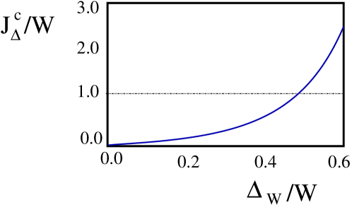
Figure 1: The critical coupling $J_{\Delta}^{c}(\Delta_{w})$ as defined in Eq.(28), as a function of $\Delta_{w}$ for $0\leq\Delta_{w}\leq 0.6$ (in units of the bandwidth $W$). As discussed in the text, the region in which Kondo regime can take place corresponds to values of $J_{\Delta}^{c}/W<1$, that is, the part of the plot lying below the dashed line, corresponding to $J_{\Delta}^{c}/W=1$.

To check the consistency between the RG flow of the running coupling and Eq.(29), we numerically compute $J_{\Delta}(D)$ vs. $D$ by integrating Eq.(26) for different values of $\Delta_{w}$. We report the corresponding curves in Fig.2a): specifically, we find that, for $\Delta_{w}=0.3$ (that is, much lower than $\Delta_{w}^{*}$), $J_{\Delta}(D)$ either flows towards the strongly coupled regime, or not, according to whether $J_{\Delta}(D_{0})>J_{\Delta}^{c}(\Delta_{w})\>(\approx 0.51)$, or $J_{\Delta}(D_{0})<J_{\Delta}^{c}(\Delta_{w})$. At variance, as it clearly appears in Fig.2b), for $\Delta_{w}>\Delta_{w}^{*}$, $J_{\Delta}(D)$ is barely renormalized by the Kondo interaction and shows no evidence of nonperturbative flow towards strong coupling.

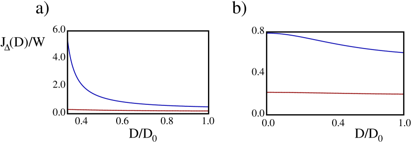
Figure 2: Renormalization Group flow of $J_{\Delta}(D)$ vs. $D$ for different values of the gap $\Delta_{w}$: a) The curves are obtained at $\Delta_{w}/W=0.3$ and for $J_{\Delta}(D_{0})/W=0.6$ (blue solid curve) and $J_{\Delta}(D_{0})/W=0.2$ (red dot-dashed curve). In this case $\Delta_{w}<\Delta_{w}^{*}$ and $J_{\Delta}^{c}(\Delta_{w})/W=0.5$: accordingly, $J_{\Delta}(D)$ flows towards strong coupling for $J_{\Delta}(D_{0})/W=0.6(>J_{\Delta}^{c}(\Delta_{w})$), while it is barely renormalized by the interaction when $J_{\Delta}(D_{0})/W=0.2(<J_{\Delta}^{c}(\Delta_{w})$; b) The curves are obtained at $\Delta_{w}/W=0.6$ and for $J_{\Delta}(D_{0})/W=0.6$ (blue solid curve) and $J_{\Delta}(D_{0})/W=0.2$ (red dot-dashed curve). Since now $\Delta_{w}>\Delta_{w}^{*}$, in neither case $J_{\Delta}(D)$ flows towards the strongly coupled regime.

Once the conditions under which the onset of the Kondo regime take place, it becomes important to infer the dependence of the corresponding Kondo temperature scale $T_{K}$ on both $J_{\Delta}(D_{0})$ and $\Delta_{w}$. By definition, one sets $T_{K}=D_{K}/k_{B}$, where $k_{B}$ is the Boltzmann constant and $D_{K}$ is the scale at which the denominator of Eq.(29) becomes equal to 0. Then, $D_{K}$ is formally given by the equation

$$1+J_{\Delta}(D_{0})\left[\frac{32}{\pi\left(1+\frac{\Delta_{w}^{2}}{W^{2}}\right)}\right]\times$$ (30)

$$\int_{\frac{\Delta_{w}}{W}}^{1}\>du\>\sqrt{u^{2}-\frac{\Delta_{w}^{2}}{W^{2}}}\sqrt{1-u^{2}}\left[\frac{1}{u^{2}+1}-\frac{1}{u^{2}+\frac{D_{K}^{2}}{W^{2}}}\right]=0\>\>\>\>.$$

As stated before, in order for the Kondo regime to take place, it is important that the condition $D_{K}/\Delta_{W}\gg 1$ is satisfied. Within such an hypothesis, we can therefore simply approximate the factor $\sqrt{u^{2}-\frac{\Delta_{w}^{2}}{W^{2}}}$ in Eq.(30) with $u$. In addition, as Kondo physics is mostly a low-energy effect, we may also approximate $\sqrt{1-u^{2}}$ simply with 1. As a result, we eventually obtain

$$T_{K}[J_{\Delta}(D_{0});\Delta_{w}]\approx D_{0}\exp\left[-\frac{\pi\left(W^{2}+\Delta_{w}^{2}\right)}{32WJ_{\Delta}(D_{0})}\right]\>\>\>\>,$$ (31)

with the cutoff $D_{0}\sim W$. As $\Delta_{w}\to 0$, Eq.(31) gives back the result for the Ising limit, once the proper correspondence between the various parameters has been traced out Giuliano et al. (2016). As s general result, Eq.(31) encodes a remarkable ”Kondo temperature renormalizazion”, namely, on increasing $\Delta_{w}$, one sees a remarkable reduction of $T_{K}$, which is consistent with the expected competition between Kondo physics and gapped spectrum Avishai et al. (2001); Choi et al. (2001); Campagnano et al. (2004); Choi et al. (2004). Specifically, Eq.(31) is expected to apply to the regime in which a nonzero $\Delta_{w}$ does not suppress Kondo effect, that is, for $D_{K}/\Delta_{w}\gg 1$. The suppression of Kondo effect with increasing $\Delta_{w}$ can instead be numerically derived, by using the integrated RG flow in Eq.(29) to estimate $T_{K}$ vs. $\Delta_{w}$ at fixed $J_{\Delta}(D_{0})$ and $T_{K}$ vs. $J_{\Delta}(D_{0})$ at fixed $\Delta_{w}$. As a result, one obtains plots such as the ones we show in Fig.3 at the system parameters chosen as discussed in the caption. In particular, the suppression of Kondo effect either on increasing $\Delta_{w}$ at fixed $J_{\Delta}(D_{0})$, or on decreasing $J_{\Delta}(D_{0})$ at fixed $\Delta_{w}$ is evidenced by the fact that the curve $T_{K}[J_{\Delta}(D_{0});\Delta_{w}]$ becomes constantly zero above (below) a critical value of $\Delta_{w}\;(J_{\Delta}(D_{0}))$ at fixed $J_{\Delta}(D_{0})\;(\Delta_{w})$.

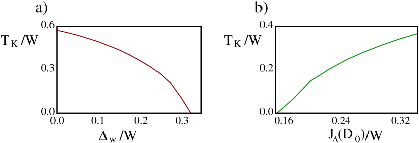
Figure 3: Full plot of the Kondo temperature as a function of $\Delta_{w}$ at fixed $J_{\Delta}(D_{0})$, and of $J_{\Delta}(D_{0})$ at fixed $\Delta_{w}$: a) $T_{K}/W$ vs. $\Delta_{w}/W$ at $J_{\Delta}(D_{0})/W=0.35$ ; b) $T_{K}/W$ vs. $J_{\Delta}(D_{0})/W$ at $\Delta_{w}/W=0.2$.

5 Majorana modes and onset of the Kondo regime

In this section we extend the perturbative RG analysis to additional terms in $H_{\Delta}$ which arise due to emergence of Majorana modes (MM)s at the endpoints of the chain. In particular, we show that, under the required assumptions for recovering Kondo effect, these terms do not affect the onset of Kondo physics. As a starting point, we note that, on including the zero-mode MM in the mode expansion of $a_{1,\lambda}+a_{1,\lambda}^{\dagger}$, Eq.(10) for $\Sigma_{1}^{\lambda}$ is modified to

$$\Sigma_{1}^{\lambda}=\rho^{2}{\cal R}^{\lambda}+\rho\omega_{1}^{\lambda}+\bar{\Sigma}_{1}^{\lambda}\>\>\>\>,$$ (32)

with $\bar{\Sigma}_{1}^{\lambda}$ contributed by nonzero modes and given by the mode expansion in Eq.(10), $\rho=\frac{\sqrt{2J^{2}-8h^{2}}}{J}=2\sqrt{2}\frac{\sqrt{\Delta_{w}W}}{J}$, and

$${\cal R}^{\lambda} = -\frac{i}{2}\sum_{\lambda^{\prime},\lambda^{{}^{\prime\prime}}}\>\epsilon^{\lambda,\lambda^{\prime},\lambda^{{}^{\prime\prime}}}\>\Gamma_{0,L}^{\lambda^{\prime}}\Gamma_{0,L}^{\lambda^{{}^{\prime\prime}}}$$

$$\omega_{1}^{\lambda} = -i\sum_{\lambda^{\prime},\lambda^{{}^{\prime\prime}}}\>\epsilon^{\lambda,\lambda^{\prime},\lambda^{{}^{\prime\prime}}}\Gamma_{0,L}^{\lambda^{{}^{\prime\prime}}}\times$$ (33)

$$\left[\sum_{\epsilon}\left(\frac{h\sin(k)}{\epsilon_{k}}\right)[\Gamma_{\epsilon_{k},\lambda^{\prime}}+\Gamma_{\epsilon_{k,\lambda^{\prime}}}^{\dagger}]\right]\>\>\>\>.$$

On inserting Eq.(32) into the expression of $H_{\Delta}$, one eventually finds

$$H_{\Delta}=H_{\Delta}^{(0)}+H_{\Delta}^{(1)}+\bar{H}_{\Delta}\>\>\>\>,$$ (34)

with

$$H_{\Delta}^{(0)} = J_{0}\>\sum_{\lambda=1}^{3}{\cal T}^{\lambda}{\cal R}^{\lambda}$$

$$H_{\Delta}^{(1)} = J_{1}\>\sum_{\lambda=1}^{3}{\cal T}^{\lambda}\omega_{1}^{\lambda}$$

$$\bar{H}_{\Delta} = \bar{J}\>\sum_{\lambda=1}^{3}{\cal T}^{\lambda}\bar{\Sigma}_{1}^{\lambda}\>\>\>\>.$$ (35)

$J_{0},J_{1}$ and $\bar{J}$ in Eq.(35) are three in principle independent running couplings which, at the bare level, are respectively given by $J_{0}=\rho^{2}J_{\Delta}$, $J_{1}=\rho J_{\Delta}$, and $\bar{J}=J_{\Delta}$. $\bar{H}_{\Delta}$ in Eq.(35) is basically the same operator as one gets in the absence of MMs. We have performed the full perturbative RG analysis of the corresponding running coupling strength $\bar{J}(D)$ in the previous section and have concluded that, under appropriate conditions on $\Delta_{w}$ $J(D_{0})$, the system can develop Kondo effect, corresponding to a marginally relevant rise of $\bar{J}(D)$, as $D$ is lowered from $D_{0}$ towards $D_{K}$. $H_{\Delta}^{(0)}$ takes the form of a ”RKKY”-like coupling between two topological spin-1/2 operators, $\vec{\cal T}$ determined by the Klein factors $\sigma^{\lambda}$, and $\vec{\cal R}$, determined by the MMs $\Gamma_{0,L}^{\lambda}$ as from Eq.(33). Based on dimensional counting arguments for boundary interaction terms Cardy (1996), one expects that, on lowering $D$, the corresponding running coupling $J_{0}(D)$ scales as $J_{0}(D)=J_{0}(D_{0})\frac{D_{0}}{D}$ and, similarly, that $J_{1}(D)$ scales as $J_{1}(D)=J_{1}(D_{0})\left(\frac{D_{0}}{D}\right)^{\frac{1}{2}}$. Apparently, on lowering $D$, this implies a rise of both $J_{0}(D)$ and $J_{1}(D)$ faster than $\bar{J}(D)$. However, one has to recall that, by definition, the scaling must be terminated at the scale $D=D_{K}$. At such a scale, one obtains

$$J_{0}(D_{K})=\rho^{2}J_{\Delta}\frac{D_{0}}{D_{K}}\sim\frac{W^{2}}{J^{2}}\frac{\Delta_{w}}{D_{K}}\>J_{\Delta}\>\>\>\>.$$ (36)

Within the magnetically ordered phase, the condition $|2h|<J$ implies $|W|/J\leq 1$. Moreover, our assumtion on the onset of the Kondo regime implies $\Delta_{w}/D_{K}\ll 1$, which eventually yields $J_{0}(D_{K})\ll J_{\Delta}$. By means of a similar argument, one readily concludes that $J_{1}(D_{K})\ll J_{\Delta}$, as well. As a result, all the way down to $D=D_{K}$, $H_{\Delta}^{(0)}$ and $H_{\Delta}^{(1)}$ merely provide a perturbative, small additional boundary interaction, which we neglect, against the relevant Kondo-like interaction $\bar{H}_{\Delta}$. It would be interesting to analyize whether it is possible to modify the Hamiltonian $H_{\Delta}$ so to eventually make the RKKY-interaction to be relevant, in the magnetically ordered phase. In fact, this would provide a tool to monitor the emergence of MMs in terms of pertinent modifications in the boundary phase diagram associated to $H_{\Delta}$ (suppression of Kondo effect). This, however, lies outside the scope of this work, and we plan to discuss it in a future publication. We thus conclude that, at least down to the scale $D=D_{K}$, the MMs do not provide sensible modification to the Kondo RG flow of the boundary coupling $J_{\Delta}(D)$, which makes the discussion of the previous section to be equally valid for the paramagnetic, as well as for the ferromagnetic phase of the spin chains.

6 Description of the strongly coupled Kondo fixed point

In the previous sections we have shown that Kondo effect in our system is recovered whenever, at a given value of $\Delta_{w}$, one has $J_{\Delta}(D_{0})>J_{\Delta}^{c}(\Delta_{w})$, implying a flow of the boundary interaction towards the strongly coupled Kondo fixed point (KFP). In this section, we provide a description of the sytem at the KFP. To do so, we combine the formal description of the KFP in the gapless case developed in Coleman et al. (1995); Giuliano and Tagliacozzo (2004) with a pertinently modified version of the projection variational approach used to study the single-channel KFP with superconducting leads Campagnano et al. (2004). The starting point is the observation that the topological spin $\vec{\cal T}$ is only coupled to the total spin density at the site $j=1$. As a consequence of the properties of the two spin-1/2 operators ${\bf S}_{j}$ and ${\bf T}_{j}$ introduced in section 3, $j=1$ hosts total spin-1/2 of ${\bf S}_{1}$ and total spin-0 of ${\bf T}_{1}$, or vice versa. As a result, when coupled to both spins by means of the 2CK-like interaction in Eq.(17), $\vec{\cal T}$ can give rise to either a total 0-spin spin singlet, or to a total spin-1 spin triplet state. In the noninteracting limit $J_{\Delta}=0$, the actual groundstate of the system is an equally-weighted mixture of singlet- and triplet-states. As $J_{\Delta}$ is turned on, we expect that, the larger is $J_{\Delta}$, the higher is the relative weight of the singlet states versus the triplet states Campagnano et al. (2004). To formally ground this observation, we define the operator ${\cal P}_{g}={\bf I}+g\sum_{\lambda=1}^{3}{\cal T}^{\lambda}\Sigma_{1}^{\lambda}$. For $g=-4$, ${\cal P}_{g}$ fully projects out the localized triplet. To set the ”optimal” value of $g$ at a given $J_{\Delta}$, one employs a variational procedure, consisting in evaluating the average value of the total Hamiltonian onto the projected out state at fixed $g$, ${\cal E}[J_{\Delta};\Delta_{w};g]$, and, at a given $J_{\Delta}$, in choosing $g$ so to minimize ${\cal E}[J_{\Delta};\Delta_{w};g]$. This determines a curve $g(J_{\Delta})$, from which one can infer what is the optimal state as $J_{\Delta}\to\infty$ (KFP). We define the projected state $|\Psi\rangle_{g}$ as

$$|\Psi\rangle_{g}=\frac{{\cal P}_{g}|{\rm GS};\Uparrow\rangle}{\sqrt{\langle{\rm GS};\Uparrow|{\cal P}_{g}^{2}|{\rm GS};\Uparrow\rangle}}\>\>\>\>,$$ (37)

with $|{\rm GS};\Uparrow\rangle=|{\rm GS}\rangle\otimes|\Uparrow\rangle$ and $|{\rm GS}\rangle$ being the groundstate of the chain Hamiltonian in Eq.(11), while $|\Uparrow\rangle$ being one of the two eigestates of ${\cal T}^{z}$ (we expect our final result not to sensibly depend on the choice of the initial state to project out, which enables us to arbitrarely choose the initial state). It is simple, now, to prove that one gets

$$\langle{\rm GS};\Uparrow|{\cal P}_{g}^{2}|{\rm GS};\Uparrow\rangle=1+\frac{3g^{2}}{16}\>\>\>\>.$$ (38)

Moreover, one also obtains

$$\langle{\rm GS};\Uparrow|{\cal P}_{g}H_{\rm Chains}{\cal P}_{g}|{\rm GS};\Uparrow\rangle$$ (39)

$$= E_{\rm GS}\left\{1+\frac{3g^{2}}{16}\right\}+3g^{2}\Psi_{1}[\Delta_{w}]\Psi_{2}[\Delta_{w}]\>\>\>\>,$$

with

$$\Psi_{1}[\Delta_{w}] = \left[\frac{1}{\pi(1+\Delta_{w})^{2}}\right]\>\int_{\Delta_{w}}^{W}\>\frac{d\epsilon}{\epsilon}\>\sqrt{\epsilon^{2}-\Delta_{w}^{2}}\sqrt{W^{2}-\epsilon^{2}}$$

$$\Psi_{2}[\Delta_{w}] = \left[\frac{1}{\pi(1+\Delta_{w})^{2}}\right]\>\int_{\Delta_{w}}^{W}\>d\epsilon\>\sqrt{\epsilon^{2}-\Delta_{w}^{2}}\sqrt{W^{2}-\epsilon^{2}}\>\>,$$

(40)

and $E_{\rm GS}=\langle{\rm GS}|H_{\rm Chain}|{\rm GS}\rangle$. In order to find out the last contribution to the averaged energy, we need the following identities

$$[\sum_{\lambda=1}^{3}\Sigma_{1}^{\lambda}{\cal R}^{\lambda}]^{2} = \frac{3}{16}-\frac{1}{4}\sum_{\lambda=1}^{3}\Sigma_{1}^{\lambda}{\cal T}^{\lambda}$$

³ $$= -\frac{3}{64}+\frac{1}{4}\sum_{\lambda=1}^{3}\Sigma_{1}^{\lambda}{\cal T}^{\lambda}\>\>\>\>.$$ (41)

Therefore, we obtain

$$\langle{\rm GS};\Uparrow|{\cal P}_{g}H_{\Delta}{\cal P}_{g}|{\rm GS};\Uparrow\rangle=\left[\frac{3g}{8}-\frac{3g^{2}}{64}\right]J_{\Delta}\>\>\>\>,$$ (42)

so that we eventually get

$${\cal E}[J_{\Delta};\Delta_{w};g]=E_{\rm GS}+\frac{3g^{2}\Psi_{1}[\Delta_{w}]\Psi_{2}[\Delta_{w}]+\frac{3}{8}g\left(1-\frac{g}{4}\right)J_{\Delta}}{1+\frac{3g^{2}}{16}}\>\>\>\>.$$ (43)

The condition $\partial_{g}{\cal E}[J_{\Delta};\Delta_{w};g]=0$ is satisfied by either setting $g=g_{1}[J_{\Delta};\Delta_{w}]$, or $g=g_{2}[J_{\Delta};\Delta_{w}]$, with

$$g_{1}[J_{\Delta};\Delta_{w}] = \frac{2{\cal H}[\Delta_{w}]-J_{\Delta}-2\sqrt{{\cal H}^{2}[\Delta_{w}]-{\cal H}[\Delta_{w}]J_{\Delta}+J_{\Delta}^{2}}}{3J_{\Delta}/4}$$

$$g_{2}[J_{\Delta};\Delta_{w}] = \frac{2{\cal H}[\Delta_{w}]-J_{\Delta}+2\sqrt{{\cal H}^{2}[\Delta_{w}]-{\cal H}[\Delta_{w}]J_{\Delta}+J_{\Delta}^{2}}}{3J_{\Delta}/4}\>\>,$$

(44)

and ${\cal H}[\Delta_{w}]=16\Psi_{1}[\Delta_{w}]\Psi_{2}[\Delta_{w}]$. In Fig.4, we plot ${\cal H}[\Delta_{w}]/W$ vs. $\Delta_{w}/W$. We see that ${\cal H}[\Delta_{w}]$ keeps finite at not-too-large values of $\Delta_{w}$. Therefore, we may readily compute $g_{j}^{*}=\lim_{J_{\Delta}\to\infty}g_{j}[J_{\Delta};\Delta_{w}]$ from Eqs.(44), obtaining $g_{1}^{*}=-4,g_{2}^{*}=\frac{4}{3}$. The latter value corresponds to projecting out the singlet and, therefore, it maximizes ${\cal E}$. Therefore, we take for good the former value which, as expected, corresponds to fully projecting out the triplet and to having a localized singlet at the effective magnetic impurity. We therefore conclude that having a nonzero $\Delta_{w}$ does not spoil Nozière’s picture of the system’s groundstate as a localized spin singlet at the impurity. As a result, we may readily describe the system’s groundstate as a twofold degenerate singlet, formed by $\vec{\cal T}$ and either one between ${\bf S}_{1}$ and ${\bf T}_{1}$ which can be simply described within our approach as discussed in Coleman et al. (1995); Giuliano and Tagliacozzo (2004).

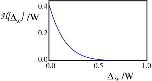
Figure 4: Plot of the function ${\cal H}[\Delta_{w}]$ vs. $\Delta_{w}$ (both quantities are measured in units of $W$).

7 Discussion and conclusions

In this paper we rigorously prove that a junction of three off-critical quantum Ising chains can be regarded as a quantum spin chain realization of the two-channel spin-1/2 overscreened Kondo effect with two superconducting leads. By making a combined use of a pertinently adapted version of poor man’s perturbative RG approach to the Kondo problem Anderson (1970); Hewson (1993) and of the variational approach to the strong coupling fixed point based on progressively projecting out from the Hilbert space states different from a localized singlet at the impurity site Campagnano et al. (2004); Giuliano and Tagliacozzo (2004), we show that, on lowering the reference energy scale $D$, the system flows all the way down to 2CK-fixed point.

Our result paves the way to the possibility of realizing and studying in a controlled setting 2CK-effect with superconducting lead, so far never considered in a solid-state quantum dot device. In fact, our proposed device appears to be within the reach of nowadays technology in nanostructures and could be engineered by means, for instance, of a pertinent Josephson junction network Giuliano and Sodano (2013). To detect the effect in the quantum spin chain system, one may look, for instance, at the scaling with $D$ of the local magnetization at the endpoints of the chains (such as discussed in Giuliano et al. (2016)). Alternatively, in the Josephson junction network realization of the system one can in principle detect the effect by means of an appropriate dc Josephson current measurement Giuliano and Sodano (2013).

Besides the theoretical interest, our results are potentially of interest for what concerns quantum entanglement properties of the system, which suggests a possible further development of our research towards quantum computation related issues. Finally, it would be interesting to study how the effect is modified by e.g. the introduction of disorded in the chains, by inhomogeneities in the boundary couplings, etc. Such a topics, though interesting, lie nevertheless beyond the scope of this work and we will possibly reserve them for a further publication.

We thank P. Sodano and A. Trombettoni for insightful discussions during the preparation of this work.

Appendix A Fermionization and explicit solution of a single quantum Ising chain with open boundary conditions

In this appendix, we review the Jordan-Wigner fermionization procedure applied to a single QIC with open boundary conditions and eventually present the exact solution of the model Hamiltonian in terms of Jordan-Wigner fermions. The Hamiltonian for a single chain is given by

$$H_{1}=-J\sum_{j=1}^{\ell-1}S_{j+1}^{x}S_{j}^{x}+h\sum_{j=1}^{\ell}S_{j}^{z}\>\>\>\>.$$ (45)

The Jordan-Wigner tranformation Jordan and Wigner (1928) allows us for trading the bosonic Hamiltonian $H_{1}$ for a fully fermionic one, by introducing a set of spinless lattice fermions $\{a_{j},a_{j}^{\dagger}\}$, obeying the basic anticommutation relations $\{a_{j},a_{j^{\prime}}^{\dagger}\}=\delta_{j,j^{\prime}}$. The relations between the bosonic spins and the fermionic operators are determined so to preserve the correct (anti)commutation relations. They are therefore given by

$$S_{j}^{+} = a_{j}^{\dagger}\>e^{i\pi\sum_{r=1}^{j-1}a_{r}^{\dagger}a_{r}}$$

$$S_{j}^{-} = a_{j}\>e^{i\pi\sum_{r=1}^{j-1}a_{r}^{\dagger}a_{r}}$$

$$S_{j}^{z} = a_{j}^{\dagger}a_{j}-\frac{1}{2}\>\>\>\>,$$ (46)

with

$$S_{j}^{x} = \frac{1}{2}[S_{j}^{+}+S_{j}^{-}]$$

$$S_{j}^{y} = \frac{-i}{2}[S_{j}^{+}-S_{j}^{-}]\>\>\>\>.$$ (47)

On inserting Eqs.(46) into the Hamiltonian in Eq.(45), we readily resort to the fully fermionized version of $H_{1}$, given by

$$H_{1}=-\frac{J}{4}\>\sum_{j=1}^{\ell-1}\{a_{j}^{\dagger}a_{j+1}+a_{j+1}^{\dagger}a_{j}\}$$ (48)

$$- \frac{J}{4}\>\sum_{j=1}^{\ell-1}\{a_{j}a_{j+1}+a_{j+1}^{\dagger}a_{j}^{\dagger}\}+h\sum_{j=1}^{\ell}a_{j}^{\dagger}a_{j}\>\>\>\>.$$

The Hamiltonian in Eq.(48) is Kitaev’s model Hamiltonian for a one-dimensional p-wave superconductor Kitaev (2001), with the various parameter (in the notation of Kitaev (2001)) chosen as $w=\Delta=\frac{J}{4}$, $\mu=-h$. To explicitly determine the energy eigenmodes of $H_{1}$, $\Gamma_{\epsilon}$, we assume that they take the form

$$\Gamma_{\epsilon} = \sum_{j=1}^{\ell}\{[u_{j}^{\epsilon}]^{*}a_{j}+[v_{j}^{\epsilon}]^{*}a_{j}^{\dagger}\}$$

$$\Gamma_{\epsilon}^{\dagger} = \sum_{j=1}^{\ell}\{v_{j}^{\epsilon}a_{j}+u_{j}^{\epsilon}a_{j}^{\dagger}\}\>\>\>\>,$$ (49)

with $u_{j}^{\epsilon},v_{j}^{\epsilon}$ being the lattice version of the quasiparticle wavefunction solving the Bogoliubov-de Gennes (BDG) equations for a superconductor de Gennes (1999). Imposing the commutation relation $[\Gamma_{\epsilon},H_{1}]=\epsilon\Gamma_{\epsilon}$, one therefore obtains the BDG equations for $(u_{j}^{\epsilon},v_{j}^{\epsilon})$, in the form

$$\epsilon u_{j}^{\epsilon} = -\frac{J}{4}\{u_{j+1}^{\epsilon}+u_{j-1}^{\epsilon}\}+\frac{J}{4}\{v_{j+1}^{\epsilon}-v_{j-1}^{\epsilon}\}+hu_{j}^{\epsilon}$$

$$\epsilon v_{j}^{\epsilon} = \frac{J}{4}\{v_{j+1}^{\epsilon}+v_{j-1}^{\epsilon}\}-\frac{J}{4}\{u_{j+1}^{\epsilon}-u_{j-1}^{\epsilon}\}-hv_{j}^{\epsilon}\>\>\>\>,$$ (50)

for $1<j<\ell$, supplemented with the boundary conditions at $j=1,\ell$ given by (see Giuliano et al. (2016) for a detailed discussion of the implementation of open boundary conditions within the fermionic description of open quantum spin chains)

$$u_{0}^{\epsilon}+v_{0}^{\epsilon}=u_{\ell+1}^{\epsilon}-v_{\ell+1}^{\epsilon}=0\>\>\>\>.$$ (51)

In solving Eqs.(50) in combination with the boundary conditions in Eq.(51), we look for solutions of the form

$$\left[\begin{array}[]{c}u_{j}^{\epsilon}\\ v_{j}^{\epsilon}\end{array}\right]=\left[\begin{array}[]{c}u_{k}\\ v_{k}\end{array}\right]e^{ikj}\>\>\>\>.$$ (52)

At a given $k$, we then find two independent solutions at energy $\pm\epsilon_{k}$, with $\epsilon_{k}=\sqrt{\frac{J^{2}}{4}+h^{2}-Jh\cos(k)}$, and the two solutions respectively given by

$$\left[\begin{array}[]{c}u_{j}^{\epsilon}\\ v_{j}^{\epsilon}\end{array}\right]_{+}=\sqrt{\frac{2}{\ell+1}}\>\left[\begin{array}[]{c}\cos\left(\frac{\varphi_{k}}{2}\right)\sin\left[kj+\frac{\varphi_{k}}{2}\right]\\ -\sin\left(\frac{\varphi_{k}}{2}\right)\cos\left[kj+\frac{\varphi_{k}}{2}\right]\end{array}\right]\;\;\;\;,$$ (53)

for the positive energy solution, with the allowed values of $k$ determined by the secular equation

$$\sin\left[k(\ell+1)+\varphi_{k}\right]=0\>\>\>\>,$$ (54)

and

$$\left[\begin{array}[]{c}u_{j}^{\epsilon}\\ v_{j}^{\epsilon}\end{array}\right]_{-}=\sqrt{\frac{2}{\ell+1}}\>\left[\begin{array}[]{c}\sin\left(\frac{\varphi_{k}}{2}\right)\cos\left[kj+\frac{\varphi_{k}}{2}\right]\\ -\cos\left(\frac{\varphi_{k}}{2}\right)\sin\left[kj+\frac{\varphi_{k}}{2}\right]\end{array}\right]\;\;\;\;,$$ (55)

for the negative-energy solution, with

$$\cos(\varphi_{k})=-\frac{\frac{J}{2}\cos(k)-h}{\epsilon_{k}}\>\>\>,\>\>\sin(\varphi_{k})=\frac{\frac{J}{2}\sin(k)}{\epsilon_{k}}\>\>\>\>.$$ (56)

with the allowed values of $k$ again given by Eq.(54). On rewriting the dispersion relation as

$$\epsilon_{k}=\sqrt{\left(\frac{J}{2}\mp h\right)^{2}+Jh\left[\cos(k)\pm 1\right]}\>\>\>\>,$$ (57)

we see that the system presents a single-fermion excitation gap $\Delta_{w}=\left|\frac{J}{2}-|h|\right|$, with quantum phase transitions at the quantum critical points $\frac{J}{2}=\pm h$ and the gap $\Delta_{w}$ correspondingly closing at $k=\pi$ or at $k=0$. The junction of quantum-critical Ising chains has been largely discussed by Tsvelik Tsvelik (2013, 2014). In the main text of this paper we instead focused onto the off-critical regime, with a fully gapped JW fermion excitation spectrum for the single chains. When the off-critical chain lies in the magnetically ordered phase, corresponding to the topological superconducting phase of Kitaev Hamiltonian (that is, within the parameter range $\frac{|2h|}{J}<1$), additional low-energy sub-gap modes arise, which, in the long-chain limit ($\ell\to\infty$) evolve into the localized zero-Majorana modes at the endpoints of the chain Kitaev (2001). Here, as we are only interested in the boundary physics at the $j=1$-boundary, we consider only the solution corresponding to the localized mode near the left-hand endpoint of the chain, with exponentially decaying wavefunction given by

$$\left[\begin{array}[]{c}u_{j}^{0}\\ v_{j}^{0}\end{array}\right]_{L}=\left[\frac{\sqrt{J^{2}-4h^{2}}}{2\sqrt{2}h}\right]\>\left[\begin{array}[]{c}1\\ -1\end{array}\right]\>\left(\frac{2h}{J}\right)^{j}\>\>\>\>.$$ (58)

As expected, the solution in Eq.(58) becomes non normalizable as $\left|\frac{2h}{J}\right|\geq 1$ and, therefore, it can no more be accepted as physically meaningful.

References

- Hewson (1993) A. C. Hewson, The Kondo problem to heavy fermions (Cambridge University Press, New York, 1993).
- Tinkham (2004) M. Tinkham, Introduction to Superconductivity (Dover Books on Physics, 2004).
- Anderson (1970) P. W. Anderson, Journal of Physics C: Solid State Physics 3, 2436 (1970).
- Buitelaar et al. (2002) M. R. Buitelaar, T. Nussbaumer, and C. Schönenberger, Phys. Rev. Lett. 89, 256801 (2002).
- Cronenwett et al. (1998) S. M. Cronenwett, T. H. Oosterkamp, and L. P. Kouwenhoven, Science 281, 540 (1998).
- Goldhaber-Gordon et al. (1998) D. Goldhaber-Gordon, H. Shtrikman, D. Mahalu, D. Abusch-Magder, U. Meirav, and M. A. Kastner, Nature 391, 156 (1998).
- Avishai et al. (2001) Y. Avishai, A. Golub, and A. D. Zaikin, Phys. Rev. B 63, 134515 (2001).
- Choi et al. (2001) M.-S. Choi, C. Bruder, and D. Loss, Physica C: Superconductivity 352, 162 (2001).
- Choi et al. (2004) M.-S. Choi, M. Lee, K. Kang, and W. Belzig, Phys. Rev. B 70, 020502 (2004).
- Campagnano et al. (2004) G. Campagnano, D. Giuliano, A. Naddeo, and A. Tagliacozzo, Physica C: Superconductivity 406, 1 (2004).
- Buizert et al. (2007) C. Buizert, A. Oiwa, K. Shibata, K. Hirakawa, and S. Tarucha, Phys. Rev. Lett. 99, 136806 (2007).
- Oguri et al. (2013) A. Oguri, Y. Tanaka, and J. Bauer, Phys. Rev. B 87, 075432 (2013).
- Lee et al. (2013) M. Lee, J. S. Lim, and R. López, Phys. Rev. B 87, 241402 (2013).
- Béri and Cooper (2012) B. Béri and N. R. Cooper, Phys. Rev. Lett. 109, 156803 (2012).
- Altland et al. (2014a) A. Altland, B. Béri, R. Egger, and A. M. Tsvelik, Phys. Rev. Lett. 113, 076401 (2014a).
- Eriksson et al. (2014) E. Eriksson, A. Nava, C. Mora, and R. Egger, Phys. Rev. B 90, 245417 (2014).
- Altland et al. (2014b) A. Altland, B. Béri, R. Egger, and A. M. Tsvelik, Journal of Physics A: Mathematical and Theoretical 47, 265001 (2014b).
- Crampè and Trombettoni (2013) N. Crampè and A. Trombettoni, Nucl. Phys. B 871, 526 (2013).
- Tsvelik (2013) A. M. Tsvelik, Phys. Rev. Lett. 110, 147202 (2013).
- Giuliano and Sodano (2013) D. Giuliano and P. Sodano, EPL (Europhysics Letters) 103, 57006 (2013).
- Giuliano et al. (2016) D. Giuliano, P. Sodano, A. Tagliacozzo, and A. Trombettoni, Nuclear Physics B 909, 135 (2016).
- Tsvelik (2014) A. M. Tsvelik, New Journal of Physics 16, 033003 (2014).
- Buccheri et al. (2015) F. Buccheri, H. Babujian, V. E. Korepin, P. Sodano, and A. Trombettoni, Nuclear Physics B 896, 52 (2015).
- Giuliano and Sodano (2007) D. Giuliano and P. Sodano, Nuclear Physics B 770, 332 (2007).
- Giuliano and Sodano (2009) D. Giuliano and P. Sodano, EPL (Europhysics Letters) 88, 17012 (2009).
- Giuliano and Sodano (2010) D. Giuliano and P. Sodano, Nuclear Physics B 837, 153 (2010).
- Cirillo et al. (2011) A. Cirillo, M. Mancini, D. Giuliano, and P. Sodano, Nuclear Physics B 852, 235 (2011).
- Jordan and Wigner (1928) P. Jordan and E. Wigner, Z. Phys. 47, 531 (1928).
- Coleman et al. (1995) P. Coleman, L. B. Ioffe, and A. M. Tsvelik, Phys. Rev. B 52, 6611 (1995).
- Alkurtass et al. (2016) B. Alkurtass, A. Bayat, I. Affleck, S. Bose, H. Johannesson, P. Sodano, E. S. Sørensen, and K. Le Hur, Phys. Rev. B 93, 081106 (2016).
- Amico et al. (2008) L. Amico, R. Fazio, A. Osterloh, and V. Vedral, Rev. Mod. Phys. 80, 517 (2008).
- Giuliano et al. (2010) D. Giuliano, A. Sindona, G. Falcone, F. Plastina, and L. Amico, New Journal of Physics 12, 025022 (2010).
- Giuliano and Tagliacozzo (2004) D. Giuliano and A. Tagliacozzo, Journal of Physics: Condensed Matter 16, 6075 (2004).
- Sachdev (2011) S. Sachdev, Quantum Phase Transitions (Cambridge University Press, New York, 2011).
- Béri (2013) B. Béri, Phys. Rev. Lett. 110, 216803 (2013).
- Dell’Anna (2010) L. Dell’Anna, Journal of Statistical Mechanics: Theory and Experiment 2010, P01007 (2010).
- Cardy (1996) J. Cardy, Scaling and Renormalization in Statistical Physics (Cambridge Lecture Notes in Physics, 1996).
- Kitaev (2001) A. Y. Kitaev, Physics-Uspekhi 44, 131 (2001).
- de Gennes (1999) P. G. de Gennes, Superconductivity Of Metals And Alloys (Westview Press, Boulder, 1999).