The OPD Photometric Survey of Open Clusters
II. robust determination of the fundamental parameters of 24 open clusters

Abstract

In the second paper of the series we continue the investigation of open cluster fundamental parameters using a robust global optimization method to fit model isochrones to photometric data. We present optical UBVRI CCD photometry (Johnsons-Cousins system) observations for 24 neglected open clusters, of which 14 have high quality data in the visible obtained for the first time, as a part of our ongoing survey being carried out in the 0.6m telescope of the Pico dos Dias Observatory in Brazil. All objects were then analyzed with a global optimization tool developed by our group which estimates the membership likelihood of the observed stars and fits an isochrone from which a distance, age, reddening, total to selective extinction ratio $R_{V}$ (included in this work as a new free parameter) and metallicity are estimated. Based on those estimates and their associated errors we analyzed the status of each object as real clusters or not, finding that two are likely to be asterisms. We also identify important discrepancies between our results and previous ones obtained in the literature which were determined using 2MASS photometry.

1 Introduction

Open clusters have long been recognized as key objects to investigate the kinematics of star formation regions, aspects of the Galactic spiral structure, or even the chemical abundance gradients in the disk of our Galaxy.

As examples of galactic parameters derived from such studies we can mention the measurement of the rotational velocity of the spiral pattern of the Galaxy by Dias & Lépine (2005), which allowed for the determination of the location of the co-rotation radius, and a lower limit of the age for the spiral pattern. The connection of the co-rotation radius and the gradient of [Fe] abundance in the Galaxy was also obtained using open clusters as discussed in Lépine et al. (2011) and Barros et al. (2013).

The efforts of our group have focused on the study of these objects throughout the last years to determine, in a systematic and consistent manner, fundamental parameters such as age, distance, reddening, metallicity and kinematical information for a large sample as possible. The main long term goal is to achieve robust statistical significance of the results obtained for open clusters. In spite of all studies that have been made, examining the DAML02 open clusters catalog (Dias et al., 2002), it is clear that much work remains to be done. Although most of the objects have estimates of the distance and age, about 50$\%$ have no reliable determination based on good quality optical photometry. The majority of clusters had parameters estimated using only near infra-red data from The Two Micron All Sky Survey (2MASS) catalog photometry. The main problem with this scenario is that 2MASS data is good for clusters which are well defined and clearly differentiated from the surrounding field which may not be always the case. Indeed as shown in Netopil et al. (2015), where the authors present a thorough analysis of the major large scale open cluster homogeneous parameters databases, there are trends or constant offsets which are significant. The authors also show that in some cases the databases can have 20% or more problematic objects, which limits the usability of these databases.

In that context, optical photometric data is still the one of the best choices to study open clusters. In this work we present 24 objects studied in our photometric Survey of Open Clusters. The survey has the goal to increase the open clusters homogeneous database with good quality observational optical data, based on UBVRI photometry performed at Pico Dos Dias Observatory - LNA/BRAZIL. The survey is described in detail in Caetano et al. (2015) (hereafter paper I). Of the 24 clusters presented, 14 have had their UBVRI data obtained for the first time.

Along with good quality observational data, the determination of fundamental parameters such as age, distance and reddening is also a key aspect of open cluster studies. In an attempt to maintain a good level of homogeneity in the determination of these parameters, we have in last years developed a tool based on global optimization techniques that removes most of the subjectivity involved in isochrone fitting while also allowing it to be reproducible within the uncertainties. The procedure allows the user to take into account important factors such as the binary fraction, initial mass function and observational uncertainties. Following the procedure outlined in detail in our previous works, the fundamental parameters for the 24 open clusters presented in this work were robustly determined from isochrone fits to the data.

Having achieved reasonable stability, we also make the code freely available to the community through a web-site dedicated to the results of this project . The code produces a wide range of output information, as stellar membership probabilities, stellar density maps, among others, which may prove to be suitable for other studies of open clusters.

The paper is organized as follows: In Sec. 2 we summarize the observational procedure, the data reduction technique as well as the transformation of the instrumental magnitudes to the standard system. In Sec. 3. we give an overview of the code and how it works and mention the main changes introduced since the last version used in Paper I. In Appendix A the details of the changes are presented. In Sec. 4 we present the color-color and color-magnitude diagrams analysis for each object and discuss the results. In Sec. 5 we give our final conclusions.

2 Observations and data reduction

All clusters targeted in the survey were observed using the same instrumental setup which is described in detailed in paper I. We used the CCD 106, a SITe SI003AB $1024\times 1024$ CCD back-illuminated camera with Johnson-Cousins UBVRI filters attached to Boller & Chivens 0.6 m telescope.

For the 14 new clusters presented in this work, images were collected in 24 through 26 of June 2010, during the same observing run which ended on the 28th June 2010. The observational strategy adopted is exactly the same as the one presented in detail in paper I, as well as the data reduction, which was performed using the softwares and techniques briefly summarized below.

All the images were pre-processed in a standard way, e.g. were trimmed, had the bias subtracted, were corrected for shutter timing effects and for sky flat field.

The instrumental magnitudes and the position of the stars in each frame were derived by the point spread function (PSF) method. We used the software STARFINDER (Diolaiti et al., 2000) which was developed for crowed stellar field analysis, adapted to be executed automatically, as described in detail in paper I.

The equatorial coordinates for each detected star were computed using the coordinates expressed in the detector reference system given by STARFINDER and the UCAC4 (Zacharias et al., 2013). The transformation between the CCD reference system and equatorial system was made through linear equations since the field is small.

2.1 Transformation to the standard system

In each night we performed observations of at least five Landolt standard fields from Clem & Landolt (2013) at different air masses. The standard fields were used to calibrate the images to the standard Johnson system considering the calibration equations given below:

$$u=U+u1+u2X+u3(U-B)$$ (1)

$$b=B+b1+b2X+b3(B-V)$$ (2)

$$v=V+v1+v2X+v3(B-V)$$ (3)

$$r=R+r1+r2X+r3(V-R)$$ (4)

$$i=I+i1+i2X+i3(V-I)$$ (5)

where upper case letters represent the magnitudes and colors in the standard system and lower case letters were adopted for the instrumental ones and X is the air mass. The coefficient values are reported in an online Table available at the web-site of the project.

The best fit was obtained by a global optimization procedure that minimized the differences between the magnitudes of the observed standard stars calculated in the standard system with those catalogued values from Clem & Landolt (2013). The final values of the coefficients are given by the mean of the results of one hundred runs of the fitting procedure and the uncertainty was estimated by the standard deviation of the solution sample. The global optimization procedure requires the definition of a parameter space which will be searched and for this we adopted typical coefficients values for the OPD site plus a range of $10\%$ to accommodate unknown variations and errors.

We present all the transformation coefficients, rms values, interesting plots as the residual of the fit to the standard stars and the errors as a function of the magnitude of all observed stars, as well as the data, in the web-site dedicated to the technical information and results of this project, and we refer the reader to it for further details.

The quality of the nights presented in this paper was checked comparing the data of the standard stars with those obtained in the night published in the paper I. The mean differences (not systematic) are typically about 0.02 mag with standard deviation lower than 0.05 mag in each filter.

3 Determining Fundamental parameters

To obtain the fundamental parameters for open clusters (age, distance, E(B-V) and metalicity) we have developed a code that employs a global optimization technique known as Cross-Entropy to perform the fitting of theoretical isochrones to photometric data. The basic procedure of the global optimization method can be summarized as follows:

1. a sample containing the initial values of the parameters to be optimized is randomly generated, according to predetermined criteria;

2. a synthetic cluster is generated for each set of parameters based on a given initial mass function and binary fraction and the theoretical isochrones of Girardi et al. (2000) and Marigo et al. (2008);

3. the synthetic cluster is compared with the observational data and a likelihood is calculated;

4. the full set of solutions is ranked based on the likelihood and a pre-defined percentage of those is selected;

5. a new sample of solutions is randomly generated, based on the distribution of the best ranked solutions of the item (iv).

6. the optimization process in items (ii) to (v) is then repeated until a stopping criteria (for example, number of iterations) is satisfied.

The procedure above is repeated for a user defined number of times performing a bootstrap procedure to re-sample with replacement the observational data. The objective is to obtain the final distribution of solutions from where we obtain the most probable one, which we adopt as the mode of the distribution. The uncertainty in the solution is the robust standard deviation of the solution sample.

The objective function used to obtain the likelihood of the solution in item (iii) is weighted by a non-parametric membership probability computed for the stars, taking into consideration their position relative to the cluster center, the star density in the particular position of the field and the multidimensional photometric data, in addition to the photometric errors. The main objective of this procedure is to minimize the subjectivity in the selection of stars and maximize the contrast of cluster features in relation to the field stars in the CMDs, allowing for a more robust fit to the available data.

The in depth code details and other relevant information are described in Oliveira et al. (2013), Dias et al. (2012), Monteiro & Dias (2011) and Monteiro et al. (2010). Also in the context of the results of the OPD Survey, we have also made a summarized discussion in Caetano et al. (2015), paper I in this series.

Since the publication of paper I we have also made several improvements to the code. We performed a general reorganization, introduced a new free parameter, the total to selective extinction ratio $R_{V}$ and implemented a way of defining the cluster region not as circle but as an iso-density region from the density map. Other minor improvements were also made aiming at making the tool publicly available. We discuss the modifications in detail in Appendix A.

For consistency, given the changes introduced in the code, we checked previously determined solutions for clusters in paper I. The comparison of our results obtained with the present version of the code to those given in the paper I shows no significant difference. The average and standard deviation of the differences of our results to those of paper I are $-0.1\pm 0.1$ mag in E(B-V), $-1\pm 332$ pc in distance, $-0.6\pm 0.2$ yr in logt, $0,005\pm 0,008$ in metallicity.

The code is written in IDL (Interactive Data Language) and has been optimized to run on multi-core on OS LINUX. A WINDOWS version is available for one core only. Basically the execution time depends on the number of the stars, number of filters, the number of the runs and the number of cores. As an example to illustrate the performance, for one hundred member stars with UBVRI data, using five i7 cores the code takes about ten hours to finalize 50 runs. As mentioned before, the code is freely available to the comunity through a web-site dedicated to the results of this project

4 Results and discussions

In this work we applied the method described previously to our UBVRI data with respective errors to determine the fundamental parameters of the studied objects. As in paper I and references therein, to make the CE more efficient in finding the global solution we adopt band $=0.15$ and $\alpha=0.4$ for the tuning parameters of the method. In practice, in each iteration $15\%$ of the best solutions were used to generate new parameter value distributions and the lower $\alpha$ value is used to slow the convergence rate of the algorithm to keep it from converging to a local minimum.

In Table 1 the code parameters used in the fitting procedure for all studied clusters are given. For all clusters $100\%$ of the stars were considered as binary. As discussed in (Monteiro et al., 2010), in the most extreme case the choice of 100% binary fraction introduces a small systematic error in the determined distance and reddening (usually within the parameter uncertainties of the fit) and does not affect the age. Ideally the binary fraction should be determined through other means and then incorporated in fitting procedure, but adopting a binary fraction of 100% essentially gives us upper limits for distance and reddening.

The tabulated isochrones used in the code were taken from Girardi et al. (2000) and Marigo et al. (2008), the same ones used in Paper I, and the parameter space was chosen as follows:

• age: from log(age) =6.60 to log(age) =10.15;

• distance: from 1 to 10 000 parsecs;

• $E(B-V)$: from 0.0 to 3.0;

• Metallicity (Z): from 0.001 to 0.30 dex with steps of $Z=0.05$ dex.

• $R_{V}$: from 2.0 to 4.0

The final value of the metallicity parameter was transformed to [Fe/H], adopting the same approximation considered in the Padova database of stellar evolutionary tracks and isochrones: $[Fe/H]=logZ/Z\odot$ with $Z\odot=0.019$. The errors were obtained by the usual propagation formula.

To determine parameter estimate errors we perform the fit for each data set 50 times, each time re-sampling from the original data set with replacement to perform a bootstrap procedure. Through this Monte-Carlo procedure new synthetic clusters are also generated each time from the theoretical isochrones using the adopted IMF. In practice this allows us to incorporate in the error estimate the effect of variations in the realizations of the synthetic clusters. The final uncertainties in each parameter are then obtained by the standard deviation of the runs.

The current version of the code can provide a series of outputs, including an estimation of the photometric membership. It also gives the user several plots that allow for a general inspection before running the full CE isochrone fit. As examples we mention important diagnostic plots such as the density map, sky chart with the proper motion of the stars, CMDs with membership, CMDs with vector proper motion overploted. Many secondary plots are also given such as the CMDs of stars inside and outside the chosen cluster region, CMDs of stars in different radii (or density selected), among others. The The Digitized Sky Survey (DSS) images may also be useful to provide independent estimates such as the radius $R_{c}$ to be used in tuning parameters. All of the plots mentioned above were used extensively in obtaining the results for the clusters in this work. In the interest of brevity we do not include all these plots here but we refer the reader to the survey web-site for the complete graphs for all studied clusters.

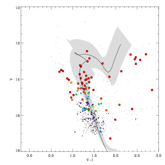
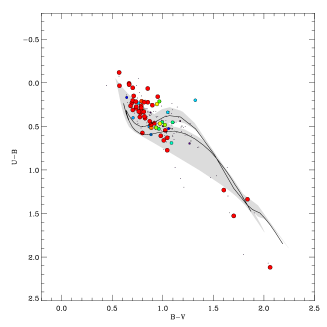
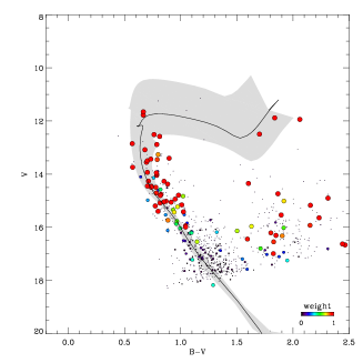
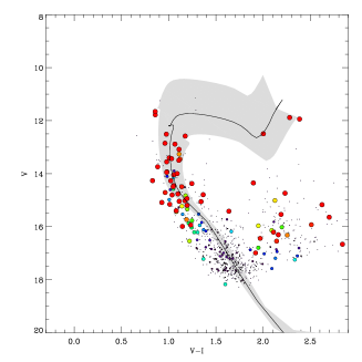
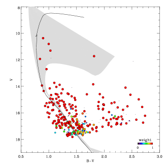
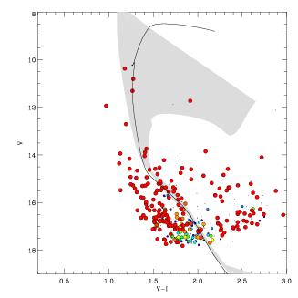
In Table 2 we present the final results for the 24 clusters investigated in this work. The isochrones fitted to the data for each cluster are shown in Figures 1 through 12 as well as Figures 14 and 17 and details are discussed below. We point out that the studied clusters in this work have not had UBVRI photometry obtained previously and fundamental parameters values available in the DAML02 catalog up to now were mostly from other authors using 2MASS data. For the 14 new clusters in this work, this is the first determination of reddening, distance, age and metallicity based on high quality CCD UBVRI photometry.

Below a detailed discussion of some of the most interesting clusters studied is presented.

4.1 Asterisms or real clusters?

As reported in paper I several candidates observed in this project may not be a real open clusters. Some cases have unclear CMDs which are difficult to analyze, even with automated statistical tools. Therefore, as in paper I, we opted to also perform a visual inspection of multiple data sources and diagnostics to provide better constrains to the code parameters used in the fitting procedure. Other more subjective criteria were also used in the final decision to indicate if the object is or not a real cluster.

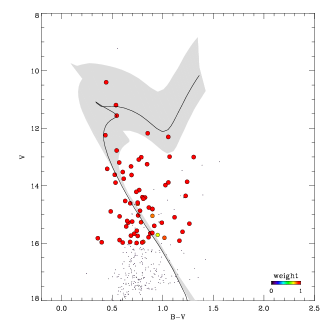
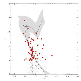
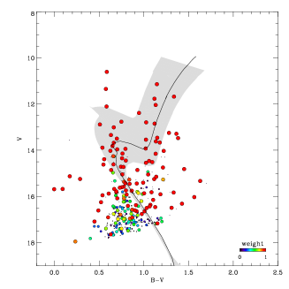
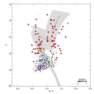
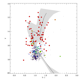
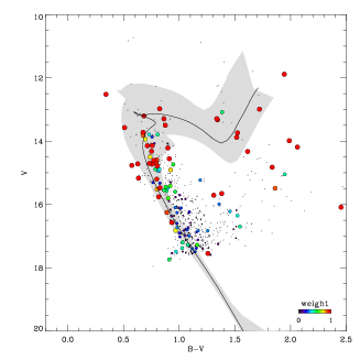
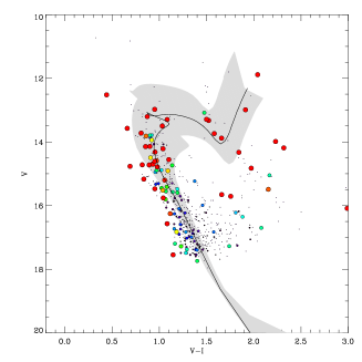
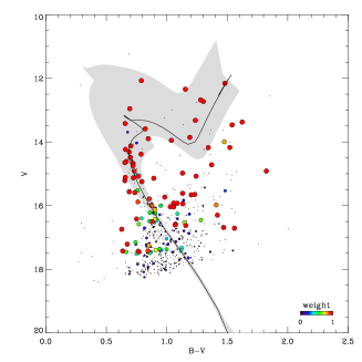
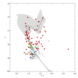
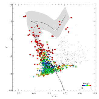
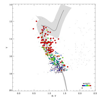
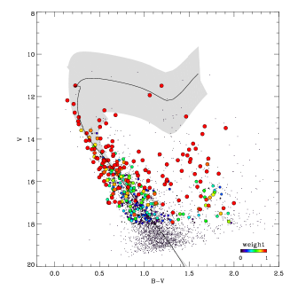
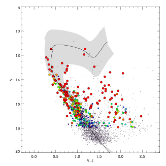
One of the first aspects we evaluate, even before performing the fit, is the CMD of the object, which we plot with the estimated photometric membership likelihood for the stars (as in Figures 1 through 12). This allows us to gauge the level of contamination present in the data and make decisions on weather restrictions in the definition of cluster area (smaller radius or higher iso-density region) will be necessary or not. It also helps in deciding if additional cuts based on color or magnitude may improve the fitting.

The second important aspect to be evaluated is the density map of the field (see for example Figure 13). With this plot we can evaluate if the over-density, which is used to automatically determine the cluster center, is clearly present. It may be the case that the over-densities cannot be separated from random density fluctuations of the non cluster stars spatial distribution. In such cases, although the code finds a fit, we tend to take lack of clear over-density as indication that the object may not be a real cluster. The density plot also lets the user decide if a radial definition of cluster region is adequate or if a iso-density would be more appropriate such as in cases where the typical King profile distribution is not present.

A third aspect which we have also incorporated in our quality control of the results is the evaluation of all the available proper motion information by visual inspection of proper motion charts combined with the CMD plot such as displayed on Figure 13. The code also produces a plot of the sky chart of the field with the proper motion vectors over-plotted. In both cases we evaluate visually if there is any coherence in the proper motion vectors, taking into account the known errors in the UCAC4 catalog. We are working in ways to implement an automation of this procedure into the code. Also related to the proper motions is the evaluation of results from kinematic analysis of Dias et al. (2014) when available where we compare proper motions to cluster proper motions obtained in that work.

A forth consideration is also made based on visual inspection of available catalog images such as those from 2MASS and most frequently the ones from DSS. In those images we are mainly searching for patterns that could be the result of stellar over-densities.

Finally, since the code produces probability distributions for the estimated parameters, we can also use this information, in particular the shape of the distributions to infer some properties of the solution. For well defined clusters the distributions are usually gaussian in shape. Distributions that tend to be flat are the result of degeneracy of that particular parameter. Large deviations from the mode are also indication of poor fits. By evaluating these properties we can subjectively decide if the procedure is fitting a real cluster or not.

When the analysis above gives contradicting results and the cluster being studied is flagged d (dubious) or nf (not found) in the DAML02 catalog, we understand that this is a strong evidence that the candidate is not a real cluster. This was the case for the objects Dolidze 33, ESO 447-29 and ESO 392-13 as discussed below.

4.2 Dolidze 33

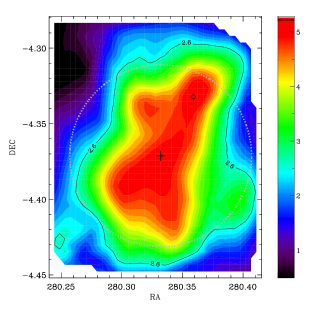
The candidate Dolidze 33 had originally a diameter of 9 arcmin and flag d (dubious) in DAML02 catalog. In Figure 13 we present the density map and the CMD with stellar vector proper motion over-plotted. Although the density map shows a region with a density 2.5 times greater than the field, the number of stars is small ($5stars/arcmin^{2}$). No initial selection criterion, either by radius or density, produced a clear signature in the CMD. There are only nine stars with $V\leq 14$ of which seven had membership greater than $51\%$. However these stars have incoherent proper motions. Finally the isochrone fit obtained by the CE (see Figure 14) is not satisfactory for the blue filters (B-V) and red filters (V-I) and does not present a Gaussian distribution of solutions for the age.

Considering the criteria mentioned above we decided to classify the Dolidze 33 as an asterism and not a real cluster.

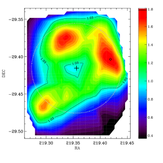
4.3 ESO 447-29

The candidate ESO 447-29 seems to be made up of the brightest stars in the observed field of about 10 arcmin. However there is no clear open cluster feature in the density map or the CMD as one can see in the Figures 4 and 15. In the density diagram the density peak is only two times greater than background as can be seen in Fig. 15. The CMD with VPDs also shows that the brightest stars of the field ($V\leq 14$) have no similar proper motion as can be seen in Fig. 15.

One issue with this cluster is that the data seem to indicate that it has a radius larger than the field of the observations. Perhaps high quality observations with a very wide field would allow us to define better the CLUSTER and FIELD populations. As it is with our available data and the considerations above we decide to classify this object as an asterism.

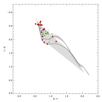
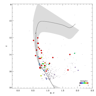
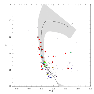
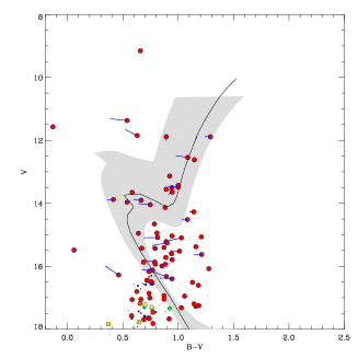
4.4 ESO 392-13

The candidate ESO 392-13 received the flag nf in the DAML02 catalog, indicating that it was not found in the visual inspection of the visual image of the DSS. In fact only one hundred stars have been detected in our observations and the density map indicates low contrast with respect to the background.

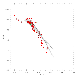
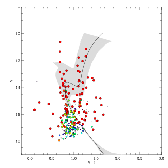
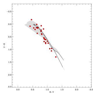
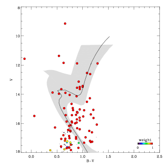
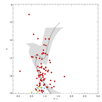
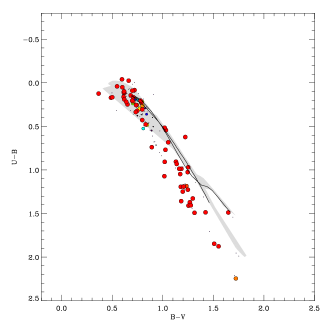
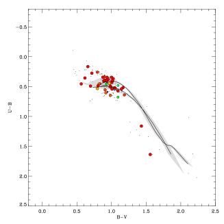
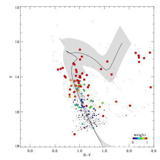
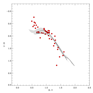
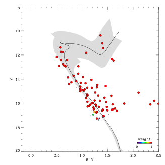
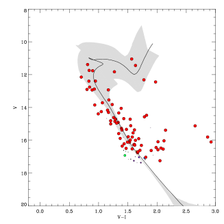
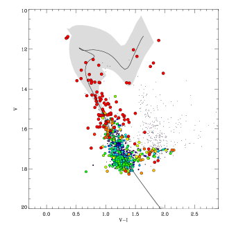
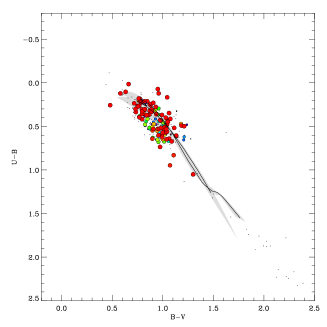
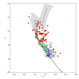
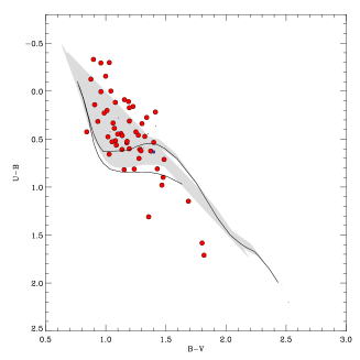
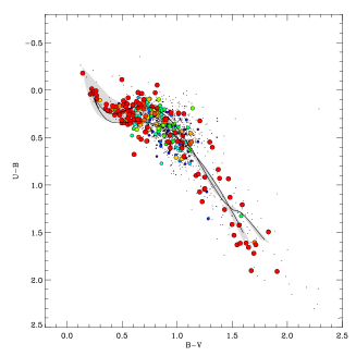
However, one interpretation of the CMD is a signature of a possible open cluster with a main sequence between $V\approx 12$ and $V\approx 19$, a turn-off $V\approx 12$ and possible giants at $(B-V)\approx 1.4$.

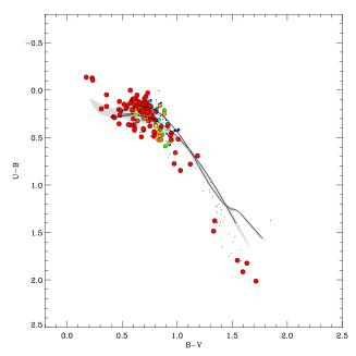
Inspecting the color-color diagram we see a group of stars with $(U-B)\leq 0.25$ and $(B-V)\leq 0.75$ that are clearly not members if we take the solution found to be true (see the Figure 9). However, eliminating those stars would leave a large gap in the main sequence that would be inconsistent with a real open cluster. This is corroborated by the inspection of the vector proper motion of that particular group showing no clear signature of group motion. Based on these considerations we classify this object as not a cluster.

4.5 Ruprecht 100

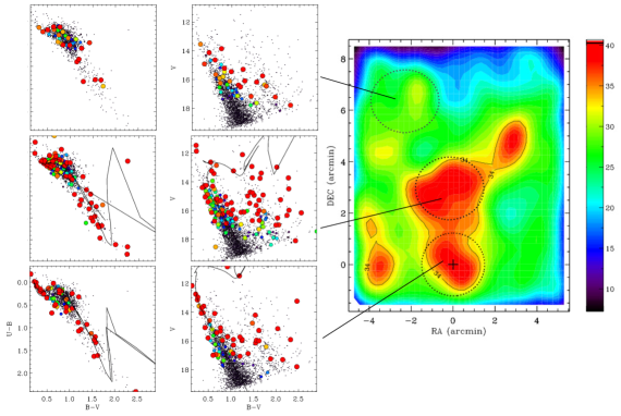
The open cluster Ruprecht 100 is an interesting case where the CMD shows two apparent populations of different ages and located about the same distance, which occur because the cluster is located toward the Sagittarius-Carina spiral arm ($l=297.7210^{\rm o}$ and $b=-0.2067^{\rm o}$). In this case, the addition of the possibility to delineate cluster regions with iso-density contours helps us to obtain a correct interpretation of the CMD and consequently a better fit to the data, as discussed below.

With the density map we can choose different regions to extract the stars initially considered as members of the cluster trying to maximize the contrast of cluster features in relation to the field stars in the CMDs. In the case of Ruprecht 100, the density map clearly shows two distinct peaks as can be seen in Fig. 16. In the fit done in Paper I, the region selected was centered on the higher density peak (middle panel in the Figure 16), with a radius of 3 arcmin and the CMD displays a turn-off at $V\approx 14$. However, we see that the secondary peak (lower panel in the Figure 16), distant about 3.5 arcmin in declination from the center, shows a population with little difference from that presented from the peak at the center of the image. In the CMD it coincides with a younger population. In the Figure 16 we also present a third region taken in the field out of the density peak which shows an expected field population.

These similarities in the two density peaks led us to the hypothesis that they are actually all part of the same cluster which does not have the classical King profile from a spherically symmetric distribution of stars. This would make the turn-off at $V\approx 14$ a contamination from the content of the Sagittarius-Carina arm, mainly constituted of a young population. In the CMD there are giants stars seen at different distances and reddening values, indicated also by the somewhat random distribution of stars with $B-V>1.5$. The final fit for this cluster presented in the Figure 17 was then done with the cluster region being defined by an iso-density region taken at 32 $star/arcmin^{2}$.

The scenario seen here is similar to the one reported by Carraro et al. (2006) for two open cluster candidates in their work, which they concluded to be just visual effects, accumulations of stars produced by the patchy nature of the inter- stellar absorption toward the Galactic bulge. Both clusters are in the Sagittarius-Carina arm region. Also according to Carraro, spatial over-densities in this direction can be effects of variable extinction. We take this discussion as evidence that indeed the cluster is a non circular structure with a slightly younger age as previously determined.

4.6 Trumpler 25

The cluster Trumpler 25 is also in the Sagittarius-Carina arm direction ($l=349.1562^{\rm o}$ and $b=-01.7738^{\rm o}$) and the scenario is similar to the one described for Ruprecht 100 (see CMD presented in Figure 7). While the density map shows a peak density, the CMD presented in the Figure 7 appears to have two distinct populations with two possible turn-offs, the younger at $V\approx 11$ and the older one at $V\approx 14$.

The analysis of the CMD with the stellar vector proper motion over-plotted show that the five stars with $V\leq 13$ and $(B-V)\leq 0.6$ that seem to represent the top of the main sequence of the younger population, show proper motions that are inconsistent with a group motion. These stars received low membership when the cluster region was defined by an iso-density region taken at about 8 $star/arcsec^{2}$.

For this case our interpretation is that the younger population is a feature of the Sagittarius-Carina arm region. It is also supported by the analysis of Carraro (2006, c.f. their Figures 12 and 13).

4.7 Comparison with the literature

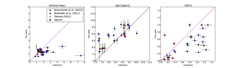
The results we obtained in this work do agree in general with other results obtained in the literature. However important discrepancies emerge when we categorize determinations from different sources. In Figure 18 we show the comparison of our results to those from the literature obtained by McSwain & Gies (2005), Kharchenko et al. (2013), Bukowiecki et al. (2011), Tadross (2011) and Carraro et al. (2006). It is clear that the best agreement to our results are from those estimates based on optical data. This is to be expected since their data set retain the higher degree of similarity to our own data, despite different isochrone fitting procedures that migh have been used. The estimates of Bukowiecki et al. (2011) and Tadross (2011) also agree well with our own even though they used 2MASS data to obtain their final parameter estimates. The results of Kharchenko et al. (2013) however show large discrepancies from our results. There are clear systematic differences in the age and E(B-V) obtained from their work. Curiously if we compare the common estimates of Bukowiecki et al. (2011) and Kharchenko et al. (2013) they do not agree among themselves, sometimes with large discrepancies beyond the uncertainties, despite the use of the same 2MASS data set. Although it is beyond the scope of this work these discrepancies warrant further investigation.

5 Conclusions

In this second paper of the series we present robust determination of the fundamental parameters of 24 open clusters from UBVRI photometry.

The code was improved in many aspects and is now more consistent with the formalism of probability distributions and a Bayesian approach to account for prior information for the stars. It is also made available for public use in a web-site developed to provide the results obtained in this project.

We presented results of the estimation of fundamental parameters of the 24 open clusters studied, 14 of which were objects for which we obtained UBVRI photometry for the first time. Some clusters were previously studied in Paper I but were re-evaluated in this work to check for the consistency of the results. The results for these clusters agree with those published in paper I, which validates the new formalism and improvements made in the code.

The results for the other clusters studied, for which we used quality UBVRI photometry obtained for the first time explore the current possibilities and limitations of the code. In particular, we emphasize that for some cases the code can work well with the automatically set parameters such as radius, density cut-off and others, but for other cases such as Ruprecht 100 or ESO 392-13 for example, a more careful analysis is necessary.

On the other hand, for some of the objects classified as clusters for which we obtained fundamental parameters, the results do not agree with previously published values in the literature derived from 2MASS data. We also found important discrepancies when comparing our results to one obtained from 2MASS photometry. In particular we also encounter important differences, not accommodated by the quoted uncertainties, between estimates from distinct authors based on the same 2MASS photometry.This subject is important and we plan to explore it further in a future study with a greater sample of open clusters for which we will have high quality UBVRI photometry.

Finally, given the fact that we have used quality UBVRI photometry, with a robust photometric membership probability estimation procedure, which takes into account the observational errors involved, we are confident that we obtained non-subjective, reliable results with realistic errors for the estimated parameters. These results will contribute to improve the open cluster information published in the DAML02 catalog available to all the community.

Appendix A Updates to the code

One of the main modification in our code was a rewrite of the algorithm that performed the non-parametric membership likelihood estimation. We have done this to make the algorithm more consistent with the formalism of probability distributions and a Bayesian approach. The motivation for the change is the possibility of incorporating new information as it becomes available in a more transparent way through clearly stated prior probabilities.

In essence the changes introduced allowed us to take the information from photometry, spatial density and distribution of stars as individual probability density functions (PDFs). These PDFs were then combined in a joint probability distribution that, after proper normalization, was used in a Bayesian hypothesis test.

The hypothesis test is based on the assumption that any given observed field of an open cluster will have stars that belong to the cluster (defined here as $H_{1}$) and others that do not (defined here as $H_{2}$). Throughout the text we also refer to stars that belong to these two distinct populations as CLUSTER and FIELD stars respectively. We also assume that the open cluster is always associated with a star density enhancement observed in a field, from which the code can determine a position which is defined as the cluster center. This position can also be set by the user if it is needed. We also assume that the further a star is from this defined center, the less likely it is to be a CLUSTER star.

This approach is more interesting from a formal point of view because it allows for missing data to be taken into account naturally. In this way if a star has no data for a given filter it will not have a PDF for it and the final probabilities are estimated based only on the available information for each star, after proper normalization.

Given the considerations above, for a given observed field the code performs the following procedures:

• with the RA and DEC coordinates of the stars the code calculates the density map using a kernel density estimate with a bandwidth determined automatically or defined by the user. The code determines automatically the bandwidth to be used based on the well known Silverman’s rule. The kernel bandwidth is then given by ${SIG\_PIX}\approx 1.06\sigma N^{-1/5}$,where $\sigma$ is the standard deviation of the sample of distance between stars and N is the number of stars.

• if not supplied by the user, from the density map the code determines the center of the cluster as the point where the density distribution peaks;

• from the RA and DEC of the stars the code determines the radius of the cluster as the standard deviation of all the distances between stars in the sample;

• with the determined radius the code separates the sample in two sub samples: CLUSTER and FIELD stars;

• from the data for each filter we determine a probability density function (PDF) and define, as in previous versions of the code, a photometric PDF given by the joint probability of all filters as $PHOT_{PDF}=U_{PDF}\times B_{PDF}\times V_{PDF}\times R_{PDF}\times I_{PDF}$. The code obtains photometric PDFs for the CLUSTER and FIELD regions respectively;

• from the density map the code obtains a PDF, $DENS_{PDF}$ using the kernel density estimate obtained in the first item;

• since we take the distance of a given star to the cluster center as an information on the membership of that star, we also adopt a PDF that describes this assuming Gaussian distribution such that $DIST_{PDF}=\frac{1}{\sqrt{2\pi\sigma^{2}}}EXP[-0.5(D_{S}/RADIUS)^{2}]$ where $D_{S}$ is the distance of star S to the center of the cluster;

• from all the information listed above the code obtains final CLUSTER and FIELD joint distributions by calculating $CLUSTER_{PDF}=DIST_{PDF}\times PHOT_{PDF}\times DENS_{PDF}$ and normalizing;

After all the steps listed above are taken, the code performs a Bayesian hypothesis test by calculating:

$$P(H_{1}\mid D)=\frac{P(D\mid H_{1})\,P(H_{1})}{P(D\mid H_{1})\,P(H_{1})\;+\;P(D\mid H_{2})\,P(H_{2})}$$ (6)

where $H_{1}$ is the hypothesis that any given star of the data set $D$ is a cluster star and $H_{2}$ is the complementary that the star is a field object. The prior probabilities $P(H_{1})$ and $P(H_{2})$ are estimated from the data considering the two populations, CLUSTER and FIELD, as determined by the code. From the star counts in the two different populations we take $P(H_{1})=n_{C}/n_{T}$ and $P(H_{2})=n_{F}/n_{T}$, where $n_{C}$ and $n_{F}$ are the number of stars in the CLUSTER and FIELD populations. $n_{T}$ is the total number of the stars in the sample. We have tested other prior probabilities but they led to minor differences in the final results.

Here we also introduced the possibility of taking the actual spatial structure of the cluster into account by allowing the CLUSTER region to be defined by an iso-density limit obtained from the density map. This tool is useful for clusters that show irregular stellar densities for which the usual King profile assumption is clearly inadequate. The procedure was critical in revising the results of the previous paper for Ruprecht 100 as discussed in Section 4.

The final result of the procedure above is to provide a membership probability for each star based on the data provided, which is then used as a weight in the global optimization procedure.

Another important addition is the inclusion of $R_{v}$ as a new free parameter. To accomplish this we implemented the detailed relations of reddening developed by Cardelli et al. (1989) which allowed us to establish the extinction values in each filter used based on a given $R_{v}$ and we refer the reader to that work for further details. The parameter space limits in this work were used in accordance with the discussion of Turner (1976) so that $2.0~{}<~{}R_{V}~{}<~{}4.0$.

Since we perform a bootstrap analysis of the fits we have access to an estimate of the probability distributions of the solutions. This in turn allows us to use the mode of the distributions to estimate final solutions to the parameters. We have implemented this feature in the current version of the code. The mode solution is now also taken to be the adopted final solution.

Table 1: The tuning parameters used in the cross-entropy fitting procedure. The first two columns (after the cluster identification) give the central coordinates. Column 4 gives the characteristic cluster radius ($R_{c}$), calculated based on the distribution of distances of each star of the sample to the center of the cluster. Column 5 gives the width ($\sigma$) of the Gaussian kernel used in the density profile. Column 6 gives $P_{cut}$, the adopted normalized cut-off. For all clusters $100\%$ of the stars were considered as binary. The values in the column radius marked with an asterisk corresponding to the density value used to select the stars.

Cluster	$\alpha_{c}$	$\delta_{c}$	radius	sig-pix	$P_{cut}$
	J2000.0	J2000.0	arcmin	arcmin
BH 217	259.071	-40.8222	1.0	1.0	0.51
Dolidze 33	280.328	-04.3797	2.5	1.0	0.95
Dolidze 35	291.36	+11.65	3.5	0.97	0.51
ESO 021-06	213.961	-78.5243	4.8	0.91	0.51
ESO 099-06	232.422	-64.8856	5.5	0.64	0.95
ESO 456-09	268.547	-32.4720	25.0*	0.55	0.90
Loden 991	206.336	-62.0311	6.0	0.77	0.95
Lynga 13	252.240	-43.4276	2.0	0.69	0.51
NGC 6588	275.200	-63.8100	3.0	0.87	0.51
Ruprecht 100	181.450	-62.6500	32.0*	0.54	0.60
BH 200	252.484	-44.1799	5.5*	0.80	0.51
ESO 008-06	223.894	-83.4423	5.5	1.06	0.51
ESO 099-06	232.471	-64.8864	5.0	0.86	0.90
ESO 139-54	271.170	-58.5388	5.0	0.85	0.90
ESO 397-01	286.037	-33.3978	5.0	0.86	0.95
ESO 447-29	219.356	-29.4155	5.5	1.00	0.90
NGC 6840	298.813	+12.1261	5.0*	0.77	0.51
Ruprecht 111	218.942	-59.9390	2.1	0.74	0.51
Trumpler 25	218.942	-59.9390	8.2*	0.74	0.51
Collinder 307	248.784	-51.0006	1.9	0.71	0.51
ESO 392-13	261.726	-34.6952	5.5	1.04	0.51
ESO 518-03	251.771	-25.8091	4.0	0.80	0.51
Loden 1002	208.562	-65.3297	5.0	0.65	0.95
Ruprecht 121	250.419	-46.1559	5.5	0.71	0.90

For Loden 991 we adopted a cut-off at $B-V\leq 0.5$. For NGC 6588 stars with $V\leq 13.5$, for ESO139-54 stars with $V\leq 16.0$. For ESO 456-09 we adopted a cut-off at $B-V\geq 1.8$ and stars with $V\leq 11.8$ received zero weight. For Ruprecht 100 we adopted a cut-off at $B-V\geq 2.0$ and stars with $V\leq 18.0$ received zero weight. For Loden 1002 stars with $B-V\geq 1.25$ and $17.0>V>14.0$ were given a weight of zero.

Table 2: Basic parameters obtained for the investigated clusters.

	This work					Literature
Cluster	$E(B-V)$	Distance	Log(Age)	Z	$R_{v}$	$E(B-V)$	Distance	Log(Age)	Ref.
	(mag)	(pc)	(yr)			(mag)	(pc)	(yr)
BH 217	$1.00\pm 0.04$	$1675\pm 182$	$7.75\pm 0.35$	$0.006\pm 0.005$	$3.02\pm 0.01$	$0.80$	$1210$	$7.54$	1
BH 217						$1.30\pm 0.10$	$1723\pm 190$	$7.54\pm 0.10$	2
BH 217						$1.15\pm 0.03$	$1693\pm 126$	$7.65\pm 0.05$	3
Dolidze 33	$0.91\pm 0.03$	$975\pm 226$	$7.70\pm 0.86$	$0.006\pm 0.005$	$3.01\pm 0.01$	$1.16\pm 0.09$	$1930\pm 212$	$7.30\pm 0.10$	2
Dolidze 35	$0.53\pm 0.06$	$869\pm 89$	$8.65\pm 0.12$	$0.027\pm 0.007$	$3.02\pm 0.05$	$1.25\pm 0.10$	$1317\pm 145$	$8.30\pm 0.05$	2
ESO 021-06	$0.04\pm 0.09$	$1426\pm 201$	$9.45\pm 0.19$	$0.027\pm 0.008$	$3.13\pm 0.04$	$0.104\pm 0.008$	$2473\pm 272$	$9.50\pm 0.05$	2
ESO 021-06						$0.21\pm 0.03$	$1745\pm 104$	$9.10\pm 0.05$	3
ESO 099-06	$0.10\pm 0.03$	$1617\pm 200$	$9.70\pm 0.24$	$0.019\pm 0.007$	$3.07\pm 0.04$	$0.229\pm 0.018$	$1274\pm 140$	$8.90\pm 0.05$	2
ESO 456-09	$0.43\pm 0.05$	$795\pm 76$	$9.05\pm 0.14$	$0.019\pm 0.007$	$3.14\pm 0.05$	$1.187\pm 0.094$	$7475\pm 822$	$10.05\pm 0.05$	2
Loden 991	$0.31\pm 0.04$	$1534\pm 127$	$9.00\pm 0.11$	$0.027\pm 0.005$	$3.04\pm 0.05$	$1.249\pm 0.100$	$2628\pm 289$	$7.25\pm 0.10$	2
Lynga 13	$0.46\pm 0.04$	$1308\pm 103$	$8.80\pm 0.14$	$0.019\pm 0.006$	$3.04\pm 0.05$	$1.041\pm 0.083$	$3412\pm 375$	$9.20\pm 0.05$	2
NGC 6588	$0.05\pm 0.01$	$2159\pm 357$	$9.65\pm 0.24$	$0.027\pm 0.008$	$3.13\pm 0.03$	$0.042\pm 0.003$	$4757\pm 523$	$9.40\pm 0.05$	2
NGC 6588						$0.10\pm 0.03$	$960\pm 44$	$9.20\pm 0.07$	4
Ruprecht 100	$0.27\pm 0.04$	$1980\pm 175$	$8.55\pm 0.24$	$0.021\pm 0.006$	$2.78\pm 0.38$	$0.729\pm 0.058$	$2589\pm 285$	$8.60\pm 0.05$	2
BH 200	$0.72\pm 0.04$	$1746\pm 208$	$7.90\pm 0.32$	$0.005\pm 0.004$	$3.03\pm 0.03$	$1.00\pm 0.03$	$1475\pm 106$	$7.35\pm 0.05$	3
ESO 099-06	$0.09\pm 0.02$	$684\pm 84$	$8.95\pm 0.41$	$0.021\pm 0.007$	$3.15\pm 0.04$	$0.229\pm 0.018$	$1274\pm 140$	$8.90\pm 0.05$	2
ESO 139-54	$0.08\pm 0.02$	$938\pm 130$	$9.00\pm 0.22$	$0.024\pm 0.007$	$3.08\pm 0.05$	$0.33\pm 0.03$	$1706\pm 105$	$9.10\pm 0.05$	3
ESO 397-01	$0.10\pm 0.03$	$1022\pm 157$	$9.65\pm 0.26$	$0.015\pm 0.007$	$3.11\pm 0.04$	$0.19\pm 0.03$	$1089\pm 65$	$9.10\pm 0.05$	3
ESO 447-29	$0.04\pm 0.02$	$1292\pm 126$	$9.60\pm 0.25$	$0.011\pm 0.007$	$3.09\pm 0.04$	$0.104\pm 0.008$	$1634\pm 180$	$9.50\pm 0.05$	2
NGC 6840	$0.16\pm 0.05$	$1296\pm 147$	$9.70\pm 0.37$	$0.015\pm 0.007$	$3.09\pm 0.05$	$0.25\pm 0.05$	$1970\pm 90$	$9.11\pm 0.03$	4
Ruprecht 111	$0.48\pm 0.04$	$1681\pm 189$	$8.90\pm 0.10$	$0.014\pm 0.007$	$3.02\pm 0.01$	$0.37\pm 0.03$	$1121\pm 70$	$9.15\pm 0.05$	3
Trumpler 25	$0.57\pm 0.06$	$1203\pm 98$	$8.90\pm 0.09$	$0.027\pm 0.006$	$3.04\pm 0.03$	$0.937\pm 0.100$	$1818$	$8.350\pm 0.05$	2
Collinder 307	$0.67\pm 0.04$	$1341\pm 155$	$8.50\pm 0.17$	$0.009\pm 0.007$	$3.06\pm 0.06$	$0.84\pm 0.10$	$1300$	$8.40$	5
Collinder 307						$0.83\pm 0.03$	$1551\pm 107$	$8.40\pm 0.05$	3
ESO 392-13	$0.44\pm 0.05$	$691\pm 104$	$8.95\pm 0.16$	$0.014\pm 0.006$	$3.12\pm 0.06$	$0.750\pm 0.100$	$816$	$7.950\pm 0.10$	2
ESO 518-03	$0.29\pm 0.03$	$1440\pm 142$	$9.05\pm 0.18$	$0.017\pm 0.006$	$3.14\pm 0.04$	$0.369\pm 0.100$	$1266$	$9.170\pm 0.05$	2
Loden 1002	$0.30\pm 0.03$	$1235\pm 183$	$9.05\pm 0.81$	$0.024\pm 0.008$	$3.19\pm 0.02$	$0.396\pm 0.100$	$1332$	$8.000\pm 0.10$	2
Ruprecht 121	$0.25\pm 0.04$	$698\pm 55$	$9.45\pm 0.22$	$0.019\pm 0.004$	$3.19\pm 0.01$	$1.041\pm 0.100$	$1239$	$8.425\pm 0.05$	2

(1) McSwain & Gies (2005); (2) Kharchenko et al. (2013); (3) Bukowiecki et al. (2011); (4) Tadross (2011); (5) Carraro 2006

Figure 1: The fit results obtained by the cross-entropy method applied to the UBVRI data for the cluster BH 200. The symbol size and color are proportional to membership of each star and are meant as a guideline only. The individual values of membership are given in the survey web-site along with other useful data. The line represents the fit of the isochrones from Girardi et al. (2000). The light-shaded region shown represents the estimated $1\sigma$ uncertainty in the fit.

Figure 2: Same as Figure 1, but for ESO139-54.

Figure 3: Same as Figure 1, but for ESO397-01.

Figure 4: Same as Figure 1, but for ESO447-29.

Figure 5: Same as Figure 1, but for NGC6840.

Figure 6: Same as Figure 1, but for Ruprecht111.

Figure 7: Same as Figure 1, but for Trumpler25.

Figure 8: Same as 1, but for Collinder307.

Figure 9: Same as Figure 1, but for ESO392-13.

Figure 10: Same as Figure 1, but for ESO518-03.

Figure 11: Same as Figure 1, but for Loden1002.

Figure 12: Same as Figure 1, but for Ruprecht121.

Figure 13: In the left panel are given the density map for the candidate Dolidze 33. Dotted line indicates the radius of the cluster and the solid line contour the density values above $1\sigma$ of the background level. In the right panel are given the CMD with the stellar vector proper motion in arbitrary units overplotted.

Figure 14: Same as Figure 1, but for Dolidze33.

Figure 15: In the left panel are given the density map for the candidate ESO 447-29. Dotted line indicates the radius of the cluster and the solid line contour the density values above $1\sigma$ of the background level. In the right panel are given the CMD with the stellar vector proper motion in arbitrary units overplotted.

Figure 16: In the right side of the panel is presented the density map of the observed region centered in the cluster Ruprecht 100. In the left side of the panel are presented the CMDs related to the marked regions in the density map. The final fit for this cluster was then done with the cluster region being defined by an iso-density region taken at 32 $star/arcmin^{2}$

Figure 17: Same as Figure 1, but for Ruprecht 100.

Figure 18: Comparison of the results obtained in this work with other determinations from the literature as listed in Table 2. The identity loci is indicated by the solid line.

References

- Barros et al. (2013) Barros, D. A., Lépine, J. R. D., & Junqueira, T. C. 2013, MNRAS, 435, 2299
- Bukowiecki et al. (2011) Bukowiecki, Ł., Maciejewski, G., Konorski, P., & Strobel, A. 2011, Acta Astron., 61, 231
- Caetano et al. (2015) Caetano, T. C., Dias, W. S., Lépine, J. R. D., et al. 2015, New A, 38, 31
- Cardelli et al. (1989) Cardelli, J. A., Clayton, G. C., & Mathis, J. S. 1989, ApJ, 345, 245
- Carraro et al. (2006) Carraro, G., Janes, K. A., Costa, E., & Méndez, R. A. 2006, MNRAS, 368, 1078
- Clem & Landolt (2013) Clem, J. L. & Landolt, A. U. 2013, AJ, 146, 88
- Dias et al. (2002) Dias, W. S., Alessi, B. S., Moitinho, A., & Lépine, J. R. D. 2002, A&A, 389, 871
- Dias & Lépine (2005) Dias, W. S. & Lépine, J. R. D. 2005, ApJ, 629, 825
- Dias et al. (2014) Dias, W. S., Monteiro, H., Caetano, T. C., et al. 2014, A&A, 564, A79
- Dias et al. (2012) Dias, W. S., Monteiro, H., Caetano, T. C., & Oliveira, A. F. 2012, A&A, 539, A125
- Diolaiti et al. (2000) Diolaiti, E., Bendinelli, O., Bonaccini, D., et al. 2000, in Astronomical Society of the Pacific Conference Series, Vol. 216, Astronomical Data Analysis Software and Systems IX, ed. N. Manset, C. Veillet, & D. Crabtree, 623
- Girardi et al. (2000) Girardi, L., Bressan, A., Bertelli, G., & Chiosi, C. 2000, A&AS, 141, 371
- Kharchenko et al. (2013) Kharchenko, N. V., Piskunov, A. E., Schilbach, E., Röser, S., & Scholz, R.-D. 2013, A&A, 558, A53
- Lépine et al. (2011) Lépine, J. R. D., Cruz, P., Scarano, Jr., S., et al. 2011, MNRAS, 417, 698
- Marigo et al. (2008) Marigo, P., Girardi, L., Bressan, A., et al. 2008, A&A, 482, 883
- McSwain & Gies (2005) McSwain, M. V. & Gies, D. R. 2005, ApJS, 161, 118
- Monteiro & Dias (2011) Monteiro, H. & Dias, W. S. 2011, A&A, 530, A91
- Monteiro et al. (2010) Monteiro, H., Dias, W. S., & Caetano, T. C. 2010, A&A, 516, A2
- Netopil et al. (2015) Netopil, M., Paunzen, E., & Carraro, G. 2015, A&A, 582, A19
- Oliveira et al. (2013) Oliveira, A. F., Monteiro, H., Dias, W. S., & Caetano, T. C. 2013, A&A, 557, A14
- Tadross (2011) Tadross, A. L. 2011, Journal of Korean Astronomical Society, 44, 1
- Turner (1976) Turner, D. G. 1976, AJ, 81, 1125
- Zacharias et al. (2013) Zacharias, N., Finch, C. T., Girard, T. M., et al. 2013, AJ, 145, 44