Proper Motion of the Leo II Dwarf Galaxy Based On
Hubble Space Telescope Imaging.

Abstract

This article reports a measurement of the proper motion of Leo II, a dwarf galaxy that is a likely satellite of the Milky Way, based on imaging with the Hubble Space Telescope and Wide Field Camera 3. The measurement uses compact background galaxies as standards of rest in both channels of the camera for two distinct pointings of the telescope and a QSO in one channel for each pointing, resulting in the weighted average of six measurements. The measured proper motion in the the equatorial coordinate system is $(\mu_{\alpha},\mu_{\delta})=(-6.9\pm 3.7,-8.7\pm 3.9)$ mas century^-1 and in the Galactic coordinate system is $(\mu_{\ell},\mu_{b})=(6.2\pm 3.9,-9.2\pm 3.7)$ mas century^-1. The implied space velocity with respect to the Galactic center is $(\Pi,\Theta,Z)=(-37\pm 38,117\pm 43,40\pm 16)$ km s^-1 or, expressed in Galactocentric radial and tangential components, $(V_{r},V_{tan})=(21.9\pm 1.5,127\pm 42)$ km s^-1. The space velocity implies that the instantaneous orbital inclination is $68^{\circ}$, with a 95% confidence interval of $(66^{\circ},80^{\circ})$. The measured motion supports the hypothesis that Leo II, Leo IV, Leo V, Crater 2, and the globular cluster Crater fell into the Milky Way as a group.

1 INTRODUCTION

Among the original seven dwarf galaxies known in the halo of the Milky Way, Leo I and Leo II are the most remote. Bellazzini et al. (2005) estimates the heliocentric distance of Leo II to be $233\pm 15$ kpc from the luminosity of the tip of the red giant branch in the $V-I$ color-magnitude diagram. Given its large distance, the question arises whether Leo II is a gravitationally-bound satellite of the Milky Way or a galaxy just passing by. Knowing the kinematics of the galaxy is necessary to answer this question. Koch et al. (2007) measured the systemic heliocentric velocity to be $79.1\pm 0.6$ km s^-1 based on radial velocities of 171 likely member stars, which is consistent with an earlier measurement of $76.0\pm 1.3$ km s^-1 (Vogt et al., 1995) based on a sample of 31 stars within the core. The radial velocity needs to be augmented with a measurement of the proper motion to obtain the instantaneous heliocentric space velocity of the dwarf. Transforming this velocity into a coordinate system at rest at the center of the Milky Way will, together with a knowledge of the Galactic potential, determine whether Leo II is bound.

Lépine et al. (2011) uses Hubble Space Telescope (HST) imaging with the Wide Field and Planetary Camera 2 and a time baseline of 14 years to make the only published measurement of the proper motion of Leo II: $(\mu_{\alpha},\mu_{\delta})=(10.4\pm 11.3,-3.3\pm 15.1)$ mas century^-1 in the equatorial coordinate system. This result is derived from the motion of 3224 likely stars of Leo II in a coordinate system defined by 17 compact background galaxies. The study assumes a distance of 230 kpc and a radial velocity of 79 km s^-1 to calculate, with additional assumptions about the Sun’s galactocentric distance and its motion with respect to the LSR, galactocentric radial and tangential velocities of $21.5\pm 4.3$ km s^-1 and $265.2\pm 129.4$ km s^-1, respectively. This velocity implies that the motion is mostly tangential; however, the uncertainty in the tangential component is large compared to typical Galactic velocities. The current work contributes a measurement with smaller uncertainty.

Deriving galactocentric motions requires adopting certain properties of Leo II and the Sun’s galactocentric distance and motion with respect to the LSR. Table 1 lists the values adopted in this article.

Table 1: Leo II and the LSR at a Glance

Quantity	Value	Reference
(1)	(2)	(3)
Right Ascension, $\alpha$ (J2000.0)	11:13:28.8	Coleman et al. (2007)
Declination, $\delta$ (J2000.0)	22:09:06.0	′′
Galactic longitude, $\ell$	$220\fdg 1691$
Galactic latitude, $b$	$+67\fdg 2313$
Ellipticity, $e$	$0.11$	′′
Core radius, $r_{c}$	$2\farcm 64\pm 0\farcm 19$	′′
Position angle, $\theta$	$6\fdg 7\pm 0\fdg 9$	′′
Heliocentric distance, $d$	$233\pm 15$ kpc	Bellazzini et al. (2005)
Heliocentric radial velocity, $v_{r}$	$79.1\pm 0.6$ km s-1	Koch et al. (2007)
$R_{LSR}$	$8.2$ kpc	Bland-Hawthorn &
$V_{LSR}$	$237$ km s-1	Gerhard (2016)
$u_{\odot}$	$-10.0\pm 1.0$ km s-1	′′
$v_{\odot}$	$11.0\pm 2.0$ km s-1	′′
$w_{\odot}$	$7.0\pm 0.5$ km s-1	′′

The organization of the rest of the article is as follows. Section 2 describes the data, Section 3 derives the proper motion, Section 4 presents the results and compares them to the previous measurement, Section 5 discusses some implications of the proper motion, and Section 6 briefly summarizes the results.

2 OBSERVATIONS AND DATA

The data consist of HST imaging for two distinct pointings in the direction of Leo II taken at two epochs that are approximately two years apart for both. This article designates them as Leo-II-1 and Leo-II-2. The detector and filter are the Wide Field Camera 3 (WFC3) and F350LP, respectively. Table 2 provides additional details. WFC3 has two 4096$\times$2051 CCDs or channels: UVIS1 and UVIS2. The direction of each pointing is that of a spectroscopically-confirmed QSO located at or near the center of UVIS1. This work uses images from both the UVIS1 and UVIS2 fields; thus, there are four distinct fields: Leo-II-1-UVIS1, Leo-II-1-UVIS2, Leo-II-2-UVIS1, and Leo-II-2-UVIS2. Figure 1 portrays the locations of the fields in a 10$\times$10 arcmin² section of the sky centered on Leo II and taken from the STScI Digitized Sky Survey.

Table 2: Information about Pointings and Images

	R.A.	Decl.	Date			Texp
Pointing	(J2000.0)	(J2000.0)	$yyyy-mm-dd$	Detector	Filter	(s)
(1)	(2)	(3)	(4)	(5)	(6)	(7)
Leo II-1	11:13:35	+22:13:02	$2010-05-12$	WFC3	F350LP	$4\times 633$
						$8\times 661$
			$2012-04-06$			$4\times 626$
						$8\times 653$
Leo II-2	11:13:41	+22:12:43	$2010-05-11$	WFC3	F350LP	$4\times 633$
						$8\times 661$
			$2012-05-01$			$4\times 626$
						$8\times 653$

Figure 1: Approximate location and orientation of the two fields in a 10$\times$10 arcmin² section of the sky centered on Leo II. North is up and East is to the left. The more northern and westward pointing is Leo-II-1. The star symbol for each pointing represents the QSO in the UVIS1 field. The dashed ellipse delineates the core of Leo-II. The values for the center, position angle, ellipticity, and core radius of the galaxy are from Table 1. Note significant overlaps among the fields.

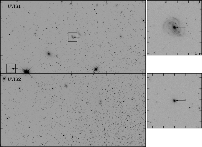
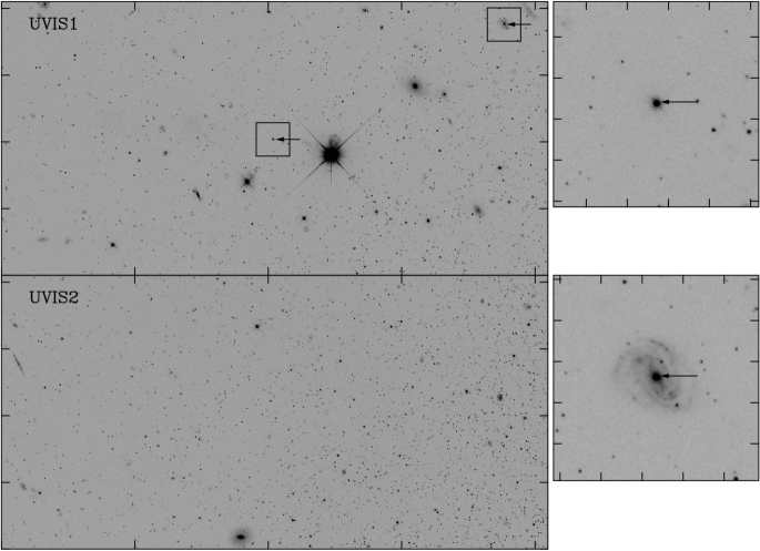
Figure 2 shows the Leo-II-1-UVIS1 (top left) and Leo-II-1-UVIS2 (bottom left) fields. Each shows the average, with cosmic ray rejection, of 12 exposures taken at the first epoch. The QSO near the center of the Leo-II-1-UVIS1 field is at the center of a $250\times 250$ pixel² box and an arrow points to it. The smaller top-right panel depicts the region of the image within this box, with the arrow again pointing to the QSO. Because of the overlap between the Leo-II-1-UVIS1 and Leo-II-2-UVIS1 fields, the QSO centered in the Leo-II-2 pointing is also present in the lower left section of Leo-II-1-UVIS1 and an arrow also points to it. A $250\times 250$ pixel² box is also centered on the QSO and the bottom right panel shows the region of the image within this box, with an arrow again pointing at the QSO. Figure 3 is analogous to Fig. 2 for the Leo-II-2 pointing.

Figure 2: The Leo-II-1-UVIS1 (top-left panel) and Leo-II-1-UVIS2 (bottom-left panel) fields. The QSO near the middle of the UVIS1 field is at the center of a $250\times 250$ pixel² box; an arrow points to the QSO and the smaller top-right panel shows the section of the image inside of this box. Another QSO in the bottom-left region of the UVIS1 field is also at the center of a $250\times 250$ pixel² box. An arrow points to this QSO and the bottom-right panel shows the section of the image inside of this box.

Figure 3: Similar to Figure 2 for the Leo-II-2-UVIS1 and Leo-II-2-UVIS2 fields.

We identified the two QSOs with photometry from the Sloan Digital Sky Survey Data Release 3 (Abazajian et al., 2005) using the method described in Richards et al. (2005) and confirmed them with spectra taken with the MMT Blue Channel Spectrograph on 2008 January 15. Q1113+2213, at the center of the Leo-II-1-UVIS1 field, has V=20.6 and the spectrum in Figure 4 implies a redshift of 0.56. Q1113+2212, at the center of the Leo-II-2-UVIS1 field, has V=21.5 and Figure 5 implies a redshift of 1.45.

Figure 4: Spectrum of Q1113+2213 in the Leo-II-1-UVIS1 field taken with the Blue Channel Spectrograph and the 300-line grating on the MMT on 2008 January 15. The spectrum covers 5200 Å, the resolution is 22 Å with the 3.5-arcsec slit, and the exposure time was 1800 s. The spectrum has been smoothed by a running mean of 9 points, which is approximately the resolution. The measured redshift is 0.56.

Figure 5: Same as Fig. 4 for Q1113+2212 in the Leo-II-2-UVIS1 field. The exposure time was 1500 s and the measured redshift is 1.45.

Measuring a proper motion involves taking images at different epochs. If the images are taken with a CCD, the degradation with time of the charge transfer efficiency (CTE) can introduce spurious motions, as shown for the STIS detector by Bristow (2004) and further discussed by Bristow et al. (2005). A degrading CTE is present in all of the CCDs, past and present, on HST. Minimizing its effect on precision astrometry has been a challenge and several techniques have been employed. 1) Numerical modeling of the charge transfer process and correcting the existing science images (Bristow & Alexov, 2002). 2) Multi-field imaging of the target with different orientations of the CCD; thus, averaging out the effects of degrading CTE (e.g., Kallivayalil et al., 2006). 3) Adopting an empirical model for how degrading CTE affects the centroid of an object as a function of its S/N and including the amplitude of this spurious shift in the fit of the transformation between the epochs (e.g., Pryor et al., 2010). 4) Pre-flashing the CCD, or introducing a “fat zero,” to fill charge traps just before the science image is taken (e.g., Anderson et al., 2012). STScI now recommends this approach for WFC3 if the average sky value is less than 12 electrons (Dressel, 2015). 5) Injection of charge into every n-th row just before the science image is taken (Bushouse et al., 2011). The injected charge fills charge traps when injected and during the readout. The current study adopts this approach — the second-epoch images have injected charge — because it eliminates the cause of CTE at its source. In the Leo-II-1-UVIS1 field, injected charge is present in every 17${}^{\mbox{th}}$ row starting with the 25${}^{\mbox{th}}$ and ending with the 2048${}^{\mbox{th}}$. This is designated as the (17, 25, 2048) injection pattern. The patterns for the remaining fields are (17, 4, 2027) for Leo-II-1-UVIS2, (17, 25, 2048) for Leo-II-2-UVIS1, and (17, 4, 2027) for Leo-II-2-UVIS2. The actual amount of charge arriving at the destination pixel depends on the history of charge loss and, possibly, charge gain as the charge packet is clocked through the CCD. The noise in the charge injection is less than expected from Poisson statistics, amounting to about 18 electrons per pixel in the injection row (Bushouse et al., 2011).

Because the first epoch data were taken soon after the installation of the WFC3, when the CTE was high, we chose not to use the charge injection option on these data, avoiding the added noise. The wide bandpass was also expected to produce significant average sky levels (they are 56-80 electrons), reducing the effect of CTE degredation. The end of Section 3.2 presents evidence that CTE losses in the first-epoch data have not had a significant impact on our results.

3 DATA REDUCTION AND ANALYSIS

Measuring a proper motion of a resolved stellar system such as Leo II from HST imaging involves two major tasks. The first is determining the most accurate centroids of stars and of bright and compact features in background galaxies. We visually inspected each galaxy. The second is matching the objects in the images at multiple epochs and deriving the relative shift between the member stars and the background galaxies and QSOs. The proper motion is proportional to this shift. The methods for both steps employed in this work are nearly identical to those in Pryor et al. (2015); thus, the current work only briefly comments on the minor differences, although it still presents the key diagnostic plots.

3.1 Measuring the Coordinates

The method for measuring the centroids of stars and galaxies employed in this work differs from that described in Pryor et al. (2015) in two ways. The first is that the correction for the geometrical distortions for the WFC3 with the F350LP filter come from Kozhurina-Platais (2014). This correction is more uncertain than those for filters used more widely, but this is automatically accounted for by the empirical estimates of our measurement uncertainties described in Sections 3.2 and 4.

The second difference is the way that the images were corrected for the degrading CTE. The current work uses the charge injection technique, described in Section 2. The standard HST pipeline uses charge-injected bias images to remove the injected charge, but the removal is incomplete. Therefore, before processing the images with DOLPHOT (Dolphin, 2000) to obtain the first estimate for a centroid and flux of an object, our method subtracts from each row with charge injection the difference between the robust (biweight) mean of the pixel values in the row and the robust mean of the pixel values in six nearby rows. The uncertainty of each pixel value in a row with charge injection is the sum in quadrature of a robust estimate of the standard deviation of the values in the row and the Poisson noise of the net signal in that pixel (the signal minus the robust row mean).

At the end of identifying objects and measuring their positions, there are 1153 objects common to the two epochs in the Leo-II-1-UVIS1 field: the central QSO, 101 selected galaxies (including the QSO in the corner), and 1051 stars with S/N greater than 10 at the first epoch. These can be succinctly written as (1153,1,101,1051). These numbers are (2330,0,145,2185) for Leo-II-1-UVIS2; (897,1,142,754) for Leo-II-2-UVIS1; and (1459,0,176,1283) for Leo-II-2-UVIS2. The S/N above is the average of the values from the individual images at an epoch. The positions of both QSOs and the galaxies are determined in the same way with templates derived from the individual images.

Figure 6 shows the uncertainty in the location of an object in the $X$ direction, $\sigma_{x}$, (top panel) and in the $Y$ direction, $\sigma_{y}$, (bottom panel) as a function of $(\mbox{S/N})^{-1}$ for the Leo-II-1-UVIS1 field. The estimate of the uncertainty in a given direction is the scatter of the transformed coordinates around their mean. The figure shows a nearly linear dependence of $\sigma_{x}$ and $\sigma_{y}$ on $(\mbox{S/N})^{-1}$, that $\sigma_{x}\approx\sigma_{y}\approx 0.01$ pixel for the stars with the highest S/N, and that $\sigma_{x}\approx\sigma_{y}\approx 0.05$ pixel for S/N = 20. The uncertainties for the other three fields are similar.

Figure 6: The rms scatter around the mean of the X-component (top panel) and the Y-component (bottom panel) of the centroid of an object as a function of $(\mbox{S/N})^{-1}$ for the first-epoch exposures in the Leo-II-1-UVIS1 field. The slanted cross is for a star and the open circle for a galaxy, with the size of the circle proportional to the FWHM of the galaxy image.

3.2 Measuring the Proper Motion

The standard coordinate system is a system co-moving with Leo II. It is defined by the locations, corrected for geometrical distortions, in the chronologically first exposure. Let $\mu_{x}$ and $\mu_{y}$ be the components of the motion of an object, in pixel yr^-1, in this system. The stars of Leo II should have $(\mu_{x},\mu_{y})$ consistent with zero, while the foreground stars and background galaxies generally should not. The exception are those few foreground stars that happen to have the same proper motion as Leo II. Contamination by Milky Way stars is unimportant in any case since the Besançon model (Robin et al., 2003) predicts fewer than 10 such stars in each of our fields. The identification of field stars is the same as in our previous articles (e.g., Pryor et al., 2015): those whose $\mu_{x}$ or $\mu_{y}$ differ from zero by a statistically significant amount (have a contribution to the $\chi^{2}$ of the fit of the transformation larger than 9.1, which corresponds approximately to a 1% chance of occurence). For the Leo II data, eliminating all trends of $\mu_{x}$ and $\mu_{y}$ with $X$ and $Y$ required the most general second-order transformation plus a cubic term in $X$. As in our previous work (e.g., Pryor et al., 2015), it is necessary to add a constant in quadrature to the coordinate uncertainties to make the $\chi^{2}$ per degree of freedom of the fitted transformation equal to one. These values range from 0.0025 pixel to 0.0042 pixel, which are similar to values found to be necessary previously. The error bars in all of the figures in this paper include these additive uncertainties.

Figure 7 shows $\mu_{x}$ (top panels) and $\mu_{y}$ (bottom panels) as a function of S/N for the Leo-II-1-UVIS1 field. The panels on the left are for the likely stars of Leo II (plus signs) and the QSO (a filled star), whereas the panels on the right are for background galaxies (filled triangles), field stars (open circles), and, again, the QSO. Similarly, Figures 8, 9, and 10 are for the other three fields. The left panels in the four figures show that the mean motion $(<\mu_{x}>,<\mu_{y}>)$ for the stars of Leo II is consistent with zero. As expected, the scatter decreases with increasing S/N. The panels on the right show that field stars have a significant motion in the standard coordinate system. These motions need not show any correlations or trends unless some of the field stars are associated with each other. The motion of the background galaxies should not show any trends with S/N; instead, the mean motion should be offset from zero by an amount proportional to the proper motion of Leo II. The points for the galaxies have a larger scatter and larger error bars than those for the stars and, thus, the offset from zero is difficult to ascertain visually.

Figure 7: Motion in the standard coordinate system, $\mu_{x}$ and $\mu_{y}$, as a function of S/N for objects in the Leo-II-1-UVIS1 field. The panels on the left are for the likely stars of Leo II (plus signs) and the QSO (filled star). The panels on the right are for the background galaxies (filled triangles), field stars (open circles), and, again, the QSO.

Figure 8: The same as Figure 7 for the Leo-II-1-UVIS2 field.

Figure 9: The same as Figure 7 for the Leo-II-2-UVIS1 field.

Figure 10: The same as Figure 7 for the Leo-II-2-UVIS2 field.

Figure 11: Motions in the standard coordinate system, $\mu_{x}$ and $\mu_{y}$, as a function of $X$ (left panels) and $Y$ (right panels) for the Leo-II-1-UVIS1 field. The symbols have the same meaning as in the previous plot.

Figure 12: The same as Figure 11 for the Leo-II-1-UVIS2 field.

Figure 13: The same as Figure 11 for the Leo-II-2-UVIS1 field.

Figure 14: The same as Figure 11 for the Leo-II-2-UVIS2 field.

The next four figures (11 — 14) show $\mu_{x}$ as a function of $X$ (top panels) and $\mu_{y}$ as a function of $Y$ (bottom panels) for the four fields in Leo II. Here, the location of an object, $(X,Y)$, is the location in the standard coordinate system. The likely stars of Leo II are at rest in this system; thus, the plus symbols representing them in the figures should show no trends with $X$ or $Y$ and have $<\mu_{x}>=0$ and $<\mu_{y}>=0$. A deviation from this distribution would be indicative of errors in determining the centroids. A visual inspection of the four figures shows no significant deviations, though the large scatter of the points may hide subtle patterns. The field stars represented by open circles show, as expected, a wide range of motions in the standard coordinate system owing to their wide range of distances and velocities with respect to the Sun and no dependence on $X$ or $Y$. The filled triangles representing the galaxies should also show no trends, though their $<\mu_{x}>$ and $<\mu_{y}>$ are expected not to be consistent with zero. A visual inspection of the figures indicates no significant trends with either $X$ or $Y$, but the large scatter of the points may hide subtle patterns.

Figures 15 — 18 are scatter plots of $(\mu_{x},\mu_{y})$ for the four fields. The top-left panel is for all of the objects; the meaning of the symbols is the same as in the previous figures, with the one difference that the size of the open circle representing a field star has been reduced to enhance the visibility of the other, more important, objects. The scale of the plot ensures that all of the objects with a measured motion are depicted. This plot should show the likely stars of Leo II scattering around $(0,0)$ with an approximately symmetric Gaussian distribution. The galaxies should have a similar, though wider, distribution, but around $(\mu_{x},\mu_{y})\neq(0,0)$. The plot in the lower-left panel of the four figures is for the field stars and galaxies only; it has the same scale as the panel above. The plot in the upper-right panel is for the likely stars of Leo II only, with a zoomed-in scale. The plot in the lower-right panel has the same scale as the one directly above and is for galaxies only.

Figure 15: Scatter plot of the measured values of $(\mu_{x},\mu_{y})$ for the objects in the Leo-II-1-UVIS1 field. Top-left panel: the plot for all of the objects. Bottom-left panel: that for the QSO, galaxies, and field stars. Top-right panel: a zoomed-in view for the likely stars of Leo II. Bottom-right panel: the same view as the above panel for the QSO and galaxies.

Figure 16: The same as Figure 15 for the Leo-II-1-UVIS2 field.

Figure 17: The same as Figure 15 for the Leo-II-2-UVIS1 field.

Figure 18: The same as Figure 15 for the Leo-II-2-UVIS2 field.

Visual inspection of the upper-right panels in Figures 15 – 18 shows that the distributions for the likely stars of Leo II are well-behaved: there are no obvious distortions from azimuthal symmetry. Similarly, examining the lower-right panels shows that the galaxies are less symmetrically distributed, though perhaps no more so than expected from their smaller number and larger scatter.

Figure 1 shows that the Leo-II-1-UVIS1 field overlaps a portion of the Leo-II-2-UVIS1 field and that the Leo-II-1-UVIS2 field overlaps portions of the Leo-II-2-UVIS1 and Leo-II-2-UVIS2 fields. Because the orientations of the fields are the same to about 0$\fdg$3, the values of $\mu_{x}$ and $\mu_{y}$ derived from different fields can be compared directly in the overlap regions. Plotting the differences of the $\mu_{x}$ values, $\Delta\mu_{x}$, or $\mu_{y}$ values, $\Delta\mu_{y}$, versus $X$, $Y$, or S/N shows no trends. The weighted means of $\Delta\mu_{x}$ and $\Delta\mu_{y}$ are zero within their uncertainties for both stars and galaxies in all three overlap regions. The $\chi^{2}$ of the scatter around these means is approximately one per degree of freedom for the galaxies when the motion uncertainties are increased as is discussed in Section 4. This argues that our final proper motion uncertainties are correct. The $\chi^{2}$ of the scatter around the mean differences for the stars is larger than one per degree of freedom, suggesting that the individual stellar motions have an additional additive uncertainty of 0.002 pixel yr^-1 — 0.008 pixel yr^-1 (8 mas century^-1 — 30 mas century^-1), depending on the region and component. We have not incorporated this additional uncertainty into our analysis because the uncertainty in the transformation to the standard coordinate system, which is determined collectively by the stars, contributes negligibly to the uncertainty for all of the final measured proper motions presented in the next section.

After the completion of the analysis reported above, a software correction for the decreasing CTE became available in the WFC3 reduction pipeline (Ryan et al., 2016). In response to a question from the referee, we repeated the analysis using the corrected first-epoch images. The resulting changes in the X- and Y-components of the mean proper motion of Leo II were 0.1 and 0.6 of their uncertainties, respectively, indicating that changes in the CTE have not significantly affected our measured proper motion. Moreover, examining the equivalents of the left-hand panels of Figures 7 — 10 clearly shows the stellar $\mu_{y}$ increasing with increasing S/N in the UVIS1 data and the reverse trend in the UVIS2 data. These trends are not present in our original figures. A more detailed examination of the data reveals that the trend is strongest for stars with smaller Y-values in UVIS1 and with larger Y-values in UVIS2. Thus, correcting for CTE losses is producing the expected pattern of changes in the stellar $\mu_{y}$ values. The surprise is that the uncorrected data show no signature of CTE losses, while the corrected data do. Perhaps the pipeline software is over-correcting the losses in the regime of our first-epoch data or perhaps the charge injection of our second-epoch data is producing an effective CTE approximately equal to that of our first epoch. In any case, the effect of CTE losses on our measured proper motion is small and we favor the value resulting from our original analysis, which is presented below.

4 RESULTS

Table 3 lists the six estimates of the proper motion in the equatorial coordinate system. In this article, $(\mu_{\alpha},\mu_{\delta})$ are the components of the proper motion in the direction of increasing right ascension and declination. Each estimate with a “g” in column (2) is derived from the mean motion of the galaxies in the standard coordinate system in the corresponding field, whereas, each estimate with a “q” is derived from the motion of the centrally-located QSO. As in Pryor et al. (2015), it is necessary to increase the uncertainties in the galaxy motions by a multiplicative factor to produce a $\chi^{2}$ per degree of freedom of one for the average galaxy motion. In the current work the factor is 1.78, 1.68, 2.27, and 1.95 for the fields Leo-II-1-UVIS1, Leo-II-1-UVIS2, Leo-II-2-UVIS1, and Leo-II-2-UVIS2, respectively. Since the QSOs were treated as galaxies, all of the uncertainties in Table 3 reflect these values.

Table 3: Measured Proper Motion of Leo II

		$\mu_{\alpha}$	$\mu_{\delta}$
Field	Ref.	(mas century-1)
(1)	(2)	(3)	(4)
Leo II-1-UVIS1	g	$-22.7\pm 8.5$	$-12.5\pm 8.7$
′′	q	$-15.9\pm 22.7$	$-16.9\pm 23.3$
Leo II-1-UVIS2	g	$-10.1\pm 7.3$	$-13.6\pm 7.8$
Leo II-2-UVIS1	g	$-1.5\pm 9.0$	$-3.6\pm 9.0$
′′	q	$4.6\pm 19.1$	$-22.3\pm 28.3$
Leo II-2-UVIS2	g	$1.9\pm 6.7$	$-3.7\pm 7.0$
Weighted mean		$-6.9\pm 3.7$	$-8.7\pm 3.9$

Figure 19 shows the measurements from Table 3 as filled triangles (galaxies) and filled stars (QSOs) together with their weighted mean (bold crossed error bars) and the measurement by Lépine et al. (2011) (open square). The weighted mean is also given in the bottom line of Table 3 and Equation 1 below. This measured proper motion of Leo II is the main result of this study.

Figure 19: The six independent estimates of the proper motion of Leo II from this study (filled triangles and stars) together with their weighted mean (bold crossed error bars), and the measurement by Lépine et al. (2011) (open square).

$$(\mu_{\alpha},\mu_{\delta})=(-6.9\pm 3.7,-8.7\pm 3.9)\ \textrm{mas}\ \textrm{century}^{-1}.$$ (1)

Comparing the six measurements of $\mu_{\alpha}$ produces a $\chi^{2}=6.3$ for five degrees of freedom, implying a probability $P=0.28$ of seeing $\chi^{2}$ equal to or larger than this value. For the corresponding measurements of $\mu_{\delta}$, $\chi^{2}=1.8$ and $P=0.88$. The agreement among the six measurements is acceptable; therefore, the uncertainties in the measured proper motion are realistic.

The measurement of the proper motion of Leo II in this work is in reasonable agreement with that from Lépine et al. (2011). The $\alpha$ components differ by 1.5 $\sigma$, while the $\delta$ components agree within their uncertainties. Our measurement has smaller uncertainties, despite the seven times shorter time baseline, because the larger passband and less-degraded CCDs produced a greater number of galaxies determining the standard of rest. The smaller pixel size and using a template constructed for each galaxy also contributed to the better astrometric precision.

Equation 2 expresses the measured proper motion of Leo II in the galactic coordinate system.

$$(\mu_{\ell},\mu_{b})=(6.2\pm 3.9,-9.2\pm 3.7)\ \textrm{mas}\ \textrm{century}^{-1}.$$ (2)

The proper motion in Equations 1 or 2 can be converted to the galactic-rest-frame (grf) proper motions $(\mu_{\alpha}^{\mbox{\tiny grf}},\mu_{\delta}^{\mbox{\tiny grf}})$ and $(\mu_{\ell}^{\mbox{\tiny grf}},\mu_{b}^{\mbox{\tiny grf}})$, which are those seen by an observer at the location of the Sun and at rest with respect to the Galactic center. In addition, one can use the proper motion to calculate the Galactocentric space velocity. The components in a cylindrical coordinate system are $\Pi$, $\Theta$, and $Z$, where $\Pi$ is positive outwards, $\Theta$ is positive in the direction of Galactic rotation, and $Z$ is positive in the direction of the north Galactic pole. The radial and tangential components in a spherical coordinate system of the Galactocentric space velocity are $V_{r}$ and $V_{t}$, respectively. Calculating the above quantities requires adopting specific values for the distance of the Sun from the Galactic center, the circular speed of the LSR, the motion of the Sun with respect to the LSR, and the distance and radial velocity of Leo II with respect to the Sun. Table 1 lists the adopted values and Table 4 the derived motions. The instantaneous space velocity implies an orbital inclination of 68^∘ with a 95% confidence interval of $(66^{\circ},80^{\circ})$. The instantaneous angular momentum vector points at $(\ell,b)=(192^{\circ},-22^{\circ})$, with a 95% confidence interval of $(149^{\circ},237^{\circ})$ for $\ell$ and $(-24^{\circ},-10^{\circ})$ for $b$.

Table 4: Derived Motions of Leo II

Quantity	Value	Comment
(1)	(2)	(3)
$(\mu_{\alpha},\mu_{\delta})^{\mbox{\tiny{Grf}}}$	$(1.7\pm 3.7,11.0\pm 3.9)$ mas century-1
$(\mu_{\ell},\mu_{b})^{\mbox{\tiny{Grf}}}$	$(-10.0\pm 3.9,5.0\pm 3.7)$ mas century-1
$(\Pi,\Theta,Z)$	$(-37\pm 38,117\pm 43,40\pm 16)$ km s-1
$V_{r}$	$21.9\pm 1.5$ km s-1
$V_{t}$	$127\pm 42$ km s-1
$i$	$68^{\circ}$ $(66^{\circ},80^{\circ})$

5 DISCUSSION

If Leo II is bound gravitationally to the Milky Way, its Galactocentric velocity provides a lower limit on the mass of the Galaxy. If the gravitational potential of the Milky Way is spherically symmetric, then the lower limit on its mass $M$ is

$$M=\frac{R(V_{r}^{2}+V_{t}^{2})}{2G},$$ (3)

where $R$ is the Galactocentric radius of the galaxy and $G$ is the universal constant of gravity. Substituting in the measured velocities from Table 4 and $R=236$ kpc gives $M=(5\pm 3)\times 10^{11}$ $M_{\odot}$. The stated uncertainty in this lower limit of the mass comes from the uncertainty in the velocity of Leo II. The location of Leo II is at about the virial radius of the Milky Way — probably slightly outside $r_{200}$ and inside $r_{vir}$ (see van der Marel et al., 2012, for example, for definitions of these quantities). Bland-Hawthorn & Gerhard (2016) reviews the observations and concludes that the virial mass of the Milky Way is $M_{vir}=(1.3\pm 0.3)\times 10^{12}\ M_{\odot}$ and $r_{vir}=282\pm 30$ kpc, which implies a mass inside the location of Leo II of $(1.2\pm 0.3)\times 10^{12}\ M_{\odot}$. The above lower limit on this mass is a factor of two below the range from observations and implies that Leo II is likely to be gravitationally bound to the Galaxy and does not provide a strong constraint on its total mass.

Torrealba et al. (2016) announced the discovery of the nearby dwarf galaxy Crater 2 and points out that this galaxy is aligned in three dimensions with the globular cluster Crater and the dwarf galaxies Leo IV, Leo V, and Leo II. The study argues that these objects were accreted as a bound group which was then tidally disrupted. If this is the case, then the Galactic-rest-frame proper motion of Leo II should be at least approximately aligned along the great circle passing through these objects. The great circle connecting Leo II and Crater 2, the two ends of the line of objects, has a position angle at the location of Leo II of $167\fdg 1$ (measured from north, through east). The equatorial galactic-rest-frame proper motion from Table 4 has a position angle of $9^{\circ}\pm 19^{\circ}$, which is $22^{\circ}$ from the great circle and, thus, is aligned within the uncertainty. The direction of motion indicates that Leo II would be leading the group. Torrealba et al. (2016) notes that the galactocentric radial velocities of the objects show that they are not on a single orbit. Instead, the orbits are co-planar with a range of energies probably acquired during the disruption of the group at perigalacticon. Thus, all of the orbits should have similar perigalacticons and the perigalacticon of Leo II should be at least as small as the smallest current Galactocentric distance of the members of the group — 120 kpc for Crater 2 (Torrealba et al., 2016). Integrating the orbit of Leo II in a fixed Galactic potential starting with the space velocity in Table 4 finds a larger perigalacticon of 161 kpc. However, the 95% confidence interval for this quantity is large, $(36,233)$ kpc, and there is a 31% chance that the perigalacticon is 120 kpc or less. Thus, the measured proper motion of Leo II is consistent with the proposal that it was part of a small group of objects which fell into the Galaxy and was tidally disrupted.

Pawlowski & Kroupa (2013) discuss the membership of the satellites of the Milky Way in the vast polar structure (VPOS). The pole of the orbit of Leo II given at the end of Section 4 allows a test of whether its orbit is aligned with the plane of the VPOS. The pole of the VPOS-3 plane is $(\ell,b)=(169\fdg 5,-2\fdg 8)$. The two poles are separated by about $29^{\circ}$, which is within the scatter of orbital poles discussed by Pawlowski & Kroupa (2013).

6 SUMMARY

We have measured the proper motion of the Leo II dwarf galaxy using images from four fields obtained with HST and WFC3 at two epochs separated by approximately two years. The measurement uses compact background galaxies and QSOs as the standard of rest.

The weighted proper motion of Leo II is $(\mu_{\alpha},\mu_{\delta})=(-6.9\pm 3.7,-8.7\pm 3.9)$ mas century^-1. The measurement from this study is in good agreement with that from Lépine et al. (2011) and has about a three times smaller uncertainty in each component.

The method of using deep multi-epoch (preferably more than two) HST imaging with compact background galaxies as the standard of rest is the best approach today for measuring the proper motions of dwarf galaxies in the halo of the Milky Way. These observations are building up a three-dimensional picture of the halo kinematics. This picture contains clues to help understand the formation of our Galaxy and its halo, galactic interactions, galactic associations (streams or planar alignments), and the amount and distribution of dark matter.

References

- Abazajian et al. (2005) Abazajian, K. et al. 2005, AJ, 129, 1755
- Anderson et al. (2012) Anderson, J., MacKenty, J., Baggett, S., & Noeski, K. 2012, “The Efficacy of Post-Flashing for Mitigating CTE-Losses in WFC3/UVIS Images” (Baltimore:STScI)
- Bellazzini et al. (2005) Bellazzini, M., Gennari, N., & Ferraro, F. R. 2005, MNRAS, 360, 185
- Bland-Hawthorn & Gerhard (2016) Bland-Hawthorn, J., & Gerhard, O. 2016, ARAA 54, 1
- Bushouse et al. (2011) Bushouse, H., Baggett, S., Gilliland, R., Noeske, K., & Petro, L. 2011, WFC3 Instrument Science Report, WFC3 ISR 2011-02
- Bristow (2004) Bristow, P. 2004, STIS Model-Based Charge Transfer Inefficiency Correction Example Science Case 1: Proper Motions of Dwarf Galaxies (CE-STIS-2004-003; Garching:ST-ECF)
- Bristow & Alexov (2002) Bristow, P., & Alexov, A. 2002, Modeling Charge Coupled Device Readout: Simulations Overview and Early Results (CE-STIS-ISR 2002; Garching:ST-ECF)
- Bristow et al. (2005) Bristow, P., Piatek, S., & Pryor, C. 2005, ST-ECF Newsletter, 38, 12
- Coleman et al. (2007) Coleman, M. G., Jordi, K., Rix, H.-W., Grebel, E. K., & Koch, A. 2007, AJ, 134, 1938
- Dolphin (2000) Dolphin, A. E. 2000, PASP, 112, 1383
- Dressel (2015) Dressel, L., 2015. “Wide Field Camera 3 Instrument Handbook, Version 7.0” (Baltimore:STScI)
- Kafle et al. (2014) Kafle, P. R., Sharma, S., Lewis, G. F., & Bland-Hawthorn, J. 2014, ApJ, 794, 59
- Kallivayalil et al. (2006) Kallivayalil, N., van der Marel, R. P., Alcock, C., Axelrod, T., Cook, K. H., Drake, A. J., & Geha, M. 2006, ApJ, 638, 772
- Koch et al. (2007) Koch, A., Kleyna, J. T., Wilkinson, M. I., Grebel, E. K., Gilmore, G. F., Wyn Evans, N., Wyse, R. F. G., & Harbeck, D. R. 2007, AJ, 134, 566
- Kozhurina-Platais (2014) Kozhurina-Platais, V. 2014, WFC3 Instrument Science Report, WFC3 ISR 2014-12 (Baltimore:STScI)
- Lépine et al. (2011) Lépine, S., Koch, A., Rich, R. M., & Kuijken, K., 2011, ApJ, 741, 100
- Pawlowski & Kroupa (2013) Pawlowski, M. S., & Kroupa, P. 2013, MNRAS, 435, 2116
- Pryor et al. (2010) Pryor, C., Piatek, S., & Olszewski, E. W. 2010, AJ, 139, 839
- Pryor et al. (2015) Pryor, C., Piatek, S., & Olszewski, E. W. 2015, AJ, 149, 42
- Richards et al. (2005) Richards, G. T. et al. 2005, MNRAS, 360, 839
- Robin et al. (2003) Robin, A. C., Reylé, C., Derrière, & Picaud, S. 2003, A&A, 409, 523
- Ryan et al. (2016) Ryan, R. E., Jr. et al. 2016, WFC3 Instrument Science Report WFC3 2016-001 (Baltimore: STScI) in WFC3 STAN, No. 22
- Torrealba et al. (2016) Torrealba, G., Koposov, S. E., Belokurov, V., & Irwin, M. 2016, MNRAS, 459, 2370
- van der Marel et al. (2012) van der Marel, R. P., Fardal, M., Besla, G., Beaton, R. L., Sohn, S. T., Anderson, J., Brown, T., & Guhathakurta, P. 2012, ApJ, 753, 8
- Vogt et al. (1995) Vogt, S. S., Mateo, M., Olszewski, E. W., & Keane, M. J. 1995, AJ, 109, 151