Radial excitations of current-carrying vortices

Abstract

We report on the existence of a new type of cosmic string solutions in the Witten model with $\mathrm{U}(1)\times\mathrm{U}(1)$ symmetry. These solutions are superconducting with radially excited condensates that exist for both gauge and ungauged currents. Our results suggest that these new configurations can be macroscopically stable, but microscopically unstable to radial perturbations. Nevertheless, they might have important consequences for the network evolution and particle emission. We discuss these effects and their possible signatures. We also comment on analogies with non-relativistic condensed matter systems where these solutions may be observable.

Introduction

Linear topological defects, e.g., vortex lines in condensed matter physics [1, 2], superfluid vortices (see e.g. [3]), non-Abelian vortices (see e.g. [4]), also frequently appear as solutions of high energy field theories where they are called cosmic strings [5]; these include grand unified (GUT) or superstring theories. Such strings yield many cosmological and astrophysical consequences [6, 7] that have not all been yet fully investigated. Many microscopic models have been discussed, providing direct contact with the underlying field theory [8].

Even in the simplest models such as the popular $\mathrm{U}(1)$ Abelian Higgs model with a Mexican hat potential, there are no known analytical solutions, straight and static ones [9] having only been constructed numerically. These so-called Abelian–Higgs or Abrikosov-Nielsen–Olesen (ANO) vortices have a localized energy-momentum tensor and a quantized magnetic-like flux with the magnetic-like field pointing in the direction of the string axis. Numerical solutions were found in Refs. [10, 11, 12] and their gravitational effects have been studied in Refs. [11, 12, 13, 14, 15, 16, 17].

The ANO string and flux tube widths are inversely proportional, respectively, to the Higgs and the gauge boson masses. When these masses are equal, the strings saturate the Bogomolonyi–Prasad–Sommerfield (BPS) bound [18] implying that the energy per unit length is proportional to the topological charge. This, in turn, guarantees stability; the fields then satisfy a set of coupled first order differential equations whose solutions are also not analytically known and thus have to be constructed numerically. Furthermore, it was shown that BPS strings remain so in curved space-time, i.e., they satisfy the same energy bound as in flat space-time [14, 15].

Cosmic strings however can be, and more often than not are [19] superconducting [20], carrying persistent currents that can be spacelike (like an ordinary current), timelike (akin to a charge), or null (chiral or lightlike [21]). Currents up to $10^{20}$ Amps (GUT case) can be induced by either bosonic or fermionic [22] charge carriers. In the former case, the scalar field that undergoes spontaneous symmetry breaking, leading to the formation of the strings, couples non-trivially to a second one. For appropriate choices of the self-couplings and vacuum expectation values of the scalar fields, the second field can form a condensate in the core of the string.

While standard cosmic strings have energy per unit length $\varepsilon$ equal to their tension $\mu$, this ceases to be true in the presence of a current. The relation between the energy per unit length and the tension of a superconducting string solution of the $\mathrm{U}(1)\times\mathrm{U}(1)$ model has been discussed in detail in [23, 24] and it has been suggested that the equation of state is of logarithmic form [25]. This has been confirmed numerically in [26]. Superconducting solutions also exist in other models, such as the semilocal $\mathrm{SU}(2)_{\rm global}\times\mathrm{U}(1)_{\rm local}$ model [27, 28] as well as in the $\mathrm{SU}(2)_{\rm local}\times\mathrm{U}(1)_{\rm local}$ electroweak model [29].

In this Letter we report on a new type of solutions in the $\mathrm{U}(1)\times\mathrm{U}(1)$ model: superconducting strings with radially excited condensates. These solutions possess a finite number of nodes in the scalar field function associated to the unbroken $\mathrm{U}(1)$ symmetry. Radial excitations of solitonic-like solutions are quite well known: they appear in non-topological soliton systems such as $Q$-balls and boson stars [30] with an unbroken symmetry as well as in topological soliton systems such as magnetic monopoles [31] in which a continuous symmetry gets spontaneously broken. To our knowledge they were so far never considered in the present context. Yet, studying the solutions of the $\mathrm{U}(1)\times\mathrm{U}(1)$ model using both analytical and numerical techniques, we find that they are a generic prediction. They are thus important to understand the mathematical structure of the theory, and may have nontrivial consequences for the evolution of the string network as well as the emission of particles during reconnection between two strings.

1 The model

We study the Witten model of superconducting strings with bosonic currents [20]. This model contains two complex scalar fields $\phi$ and $\sigma$ which are minimally coupled to two (different) U(1) gauge fields. Using a metric with signature $(+,-,-,-)$, the Lagrangian density reads

$$\mathcal{L}= -\frac{1}{4}F_{\mu\nu}F^{\mu\nu}-\frac{1}{4}G_{\mu\nu}G^{\mu\nu}+\frac{1}{2}D_{\mu}\phi\left(D^{\mu}\phi\right)^{*}$$

$$+\frac{1}{2}D_{\mu}\sigma\left(D^{\mu}\sigma\right)^{*}-V(\phi,\sigma),$$ (1)

where the potential is given by

$$V(\phi,\sigma)=\frac{\lambda_{1}}{4}(|\phi|^{2}-\eta_{1}^{2})^{2}+\frac{\lambda_{2}}{4}|\sigma|^{2}(|\sigma|^{2}-2\eta_{2}^{2})+\frac{\lambda_{3}}{2}|\phi|^{2}|\sigma|^{2},$$ (2)

the gauge covariant derivatives read

$$D_{\mu}\phi=\left(\partial_{\mu}-\mathsf{i}\,e_{\phi}B_{\mu}\right)\phi\ \ ,\ \ D_{\mu}\sigma=\left(\partial_{\mu}-\mathsf{i}\,e_{\sigma}A_{\mu}\right)\sigma\ ,$$ (3)

and the field strength tensors of the two U(1) gauge fields $A_{\mu}$ and $B_{\mu}$ are

$$G_{\mu\nu}=\partial_{\mu}B_{\nu}-\partial_{\nu}B_{\mu}\ \ ,\ \ F_{\mu\nu}=\partial_{\mu}A_{\nu}-\partial_{\nu}A_{\mu}\ .$$ (4)

In the following we will use cylindrical coordinates $(t,r,\theta,z)$ and work with the ansatz

$$B_{\mu}\mbox{d}x^{\mu}=\frac{1}{e_{\phi}}\left[n-P\left(r\right)\right]\mbox{d}\theta\ ,\ \phi(r,\theta)=\eta_{1}h(r)\,\mbox{e}^{\mathsf{i}n\theta}\ ,\$$

$$A_{\mu}\mbox{d}x^{\mu}=A_{z}(r)\mbox{d}z+A_{t}(r)\mbox{d}t\ ,\ \sigma(t,r,z)=\eta_{1}f(r)\,\mbox{e}^{\mathsf{i}(\omega t-kz)}.$$ (5)

From now on, we shall restrict attention to the case $e_{\sigma}=0$, for which the external gauge field $A_{\mu}$ can be set to zero as well; in fact, this gauge field is sourced by the current flowing along the string but hardly backreacts on the string microstructure [24]. In Section 4 we briefly comment on the case $e_{\sigma}\neq 0$.

Introducing the dimensionless coordinate $x:=\sqrt{\lambda_{1}}\eta_{1}r$, the equations of motion only depend on the dimensionless coupling constants

$$\alpha^{2}=\frac{e_{\phi}^{2}}{\lambda_{1}}\ ,\ q=\frac{\eta_{2}}{\eta_{1}}\ ,\ \gamma_{i}=\frac{\lambda_{i}}{\lambda_{1}}\ \ (i=2,3),$$ (6)

as well as the (also dimensionless) state parameter $w:=(k^{2}-\omega^{2})/(\lambda_{1}\eta_{1}^{2})$; they read

$$\left(\frac{P^{\prime}}{x}\right)^{\prime} =\alpha^{2}\frac{Ph^{2}}{x}\ ,$$ (7)

$$\frac{1}{x}\left(xh^{\prime}\right)^{\prime} =h\left(\frac{P^{2}}{x^{2}}+h^{2}-1+\gamma_{3}f^{2}\right)\ ,$$ (8)

$$\frac{1}{x}\left(xf^{\prime}\right)^{\prime} =f\left[w+\gamma_{2}\left(f^{2}-q^{2}\right)+\gamma_{3}h^{2}\right],$$ (9)

where a prime denotes a derivative with respect to $x$. The boundary conditions at the string axis $x=0$ and at infinity read

$$P(x)|_{x=0} =n\ ,\ h(x)|_{x=0}=0\ ,\ f^{\prime}(x)|_{x=0}=0\ ,$$

$$\lim_{x\rightarrow\infty}P(x) =0\ ,\lim_{x\rightarrow\infty}h(x)=1\ ,f(x)\mathop{=}_{x\to\infty}o\left(x^{-1/2}\right)$$ (10)

The important physical quantities of the solutions are the energy per unit length $\varepsilon$ and the tension $\mu$, given (in rescaled units) by

$$\varepsilon=-2\pi\int xT^{t}_{t}\,\mbox{d}x\ \ ,\ \ \mu=-2\pi\int xT^{z}_{z}\,\mbox{d}x\ ,$$ (11)

respectively, with the energy-momentum tensor

$$T_{\mu\nu}=-2\frac{\delta\mathcal{L}}{\delta g^{\mu\nu}}+g_{\mu\nu}\mathcal{L}\ ,$$ (12)

as well as the (rescaled) absolute value $I$ of the current :

$$I=2\pi\sqrt{|w|}\int xf^{2}\,\mbox{d}x\ .$$ (13)

Note that our model bears strong similarities with that of Ref. [32] provided one makes the replacements $\eta_{1}\to 1$, $\beta_{1}\to 2\lambda_{1}$, $\beta_{2}\to\lambda_{2}/2$, $\beta^{\prime}\to\lambda_{3}/2$ and $\alpha\to\lambda_{2}\eta_{2}^{2}/2$; it was shown that different types of solutions may exist in this model, but for the purpose of exhibiting our new configuration, we shall only consider the regime of parameters for which the corresponding ANO vortices (without currents) under consideration are of type II [7] and restrict attention to the case $n=1$ for simplicity.

2 Small condensates

To motivate the existence of excited solutions, let us first consider the regime where the condensate is sufficiently small that we can neglect the term $\propto f^{3}$ in (9) as well as the back-reaction on $h$, i.e. the term $\propto f^{2}$ in (8). Assuming the currentless ANO vortex to be stable (hence choosing $n=1$), we follow the analysis of Witten [20] and perturb the scalar field $\sigma$ around $\sigma(x)\equiv 0$ in the background of this vortex. This will tell us whether in a given setting the vortex can sustain the additional structure.

Taking the boundary conditions into account, we assume the following simple ansatz for the Higgs field function

$$h(x)=\left\{\begin{array}[]{lll}\kappa\,x&{\rm for}&0\leq x<1/\kappa,\\ 1&{\rm for}&1/\kappa\leq x,\end{array}\right.$$ (14)

where $\kappa$ is a freely adjustable constant giving the characteristic size of the Higgs field variations. For $x\geq 1/\kappa$, equation (9) then becomes

$$\frac{1}{x}\left(x\,f^{\prime}\right)^{\prime}=\left(w-\gamma_{2}\,q^{2}+\gamma_{3}\right)f.$$ (15)

This is a modified Bessel equation whose only solution decaying strictly faster that $x^{-1/2}$ at infinity is

$$f(x)=C_{1}K_{0}\left(\sqrt{w-\gamma_{2}q^{2}+\gamma_{3}}\,x\right)\ ,$$ (16)

where $C_{1}\in\mathbb{R}$ is an integration constant and $K_{0}$ is the zeroth order modified Bessel function of the second kind. In the interior region $x<1/\kappa$, equation (9) becomes

$$\frac{1}{x}\left(x\,f^{\prime}\right)^{\prime}=\left(w-\gamma_{2}\,q^{2}+\gamma_{3}\,\kappa\,x\right)f.$$ (17)

To find its solutions, it is useful to define the variable $Y(x)$ and the function $F$ by

$$Y(x)\equiv\sqrt{\gamma_{3}}\kappa x^{2},\ \ F\left[Y(x)\right]=\exp\left[\frac{Y(x)}{2}\right]f(x).$$ (18)

Equation (17) is then rewritten as the linear, second order differential equation

$$Y\frac{\mbox{d}^{2}F}{\mbox{d}Y^{2}}+(1-Y)\frac{\mbox{d}F}{\mbox{d}Y}+m\,F=0\ ,$$ (19)

where

$$m\equiv-\left(\displaystyle\frac{w-\gamma_{2}q^{2}}{4\sqrt{\gamma_{3}}\kappa}+\frac{1}{2}\right)\ .$$ (20)

Eq. (19) is the confluent hypergeometric equation [34]. It has only one regular solution at the origin, namely $F(Y)=C_{2}L_{m}(Y)$, where $L_{m}$ denotes the Laguerre function with parameter $m$ and $C_{2}\in\mathbb{R}$ is another integration constant. So, for $x<1/\kappa$, the only regular solution of (17) is

$$f(x)=C_{2}\,\mbox{e}^{-\sqrt{\gamma_{3}}\kappa x^{2}/2}L_{m}(\sqrt{\gamma_{3}}\kappa x^{2}),\,C_{2}\in\mathbb{R}.$$ (21)

The requirement that $f$ and $f^{\prime}$ should be continuous at $x=1/\kappa$ gives two matching conditions. The first one is a relation between $C_{1}$ and $C_{2}$. The other one gives a constraint on $m$ with a discrete set of solutions (see [33] for more details.) That is, regular solutions decaying sufficiently fast at infinity exist only for these discrete values of $m$, which was to be expected since the linearized version of Eq. (9) solved here is nothing but a two dimensional Schrödinger equation in a confining potential with a finite number of bound states.

In the limit $\sqrt{\gamma_{3}}/\kappa\to\infty$, these solutions are localized in the domain $x\ll 1/\kappa$, so that (21) is valid up to a region where $f$ is exponentially small. Regular solutions are then given in terms of the Laguerre polynomials [34], restricting $m$ to be a natural integer. As the $m^{\rm th}$ Laguerre polynomial has $m$ strictly positive roots, the corresponding function $f$ has $m$ nodes (see Fig. 1, dashed lines for $m=1$ and $m=2$). In practice, the finite value of $\kappa$ gives a cutoff on $m$, of the order of $\sqrt{\gamma_{3}}/(4\kappa)$. For the numerical solutions shown in the figure, we estimate that $\sqrt{\gamma_{3}}/(4\kappa)\approx 4.90$ for $m=1$ and $\sqrt{\gamma_{3}}/(4\kappa)\approx 4.32$ for $m=2$, respectively. Since nonlinear effects tend to reduce the number of solutions, we thus expect to have a few of them when working with the full set of equations. This is compatible with the fact that for these parameters, only solutions with $0$, $1$, and $2$ nodes exist, see the next section. In the following, for simplicity we denote by $m$ the number of nodes of the function $f$, although it does not exactly follow (21).

The existence of bound states around an otherwise stable ANO vortex is the reason why an ordinary cosmic string can become superconducting [20]. Our discussion here goes one step further by showing that there is a finite number of such bound states, each of which leading to an instability in the current condensate, an instability that will be tamed by the nonlinear terms: one therefore expects that for each value of $w$, the full nonlinear set of equations should lead to a series of solutions with finite energy per unit length and tension in the form of a ground state and excited modes.

Indeed, so far, we have worked to linear order in $f$. When including the nonlinear term $\propto f^{3}$ and its backreaction on $h$ and $P$, the amplitude of the regular, asymptotically decaying solutions depends on the values of $w$. Since the boundary conditions and asymptotic behaviors of bounded solutions remain similar to the linear case, one can conjecture they remain discrete, and can be continuously deformed into the linear solutions, so it seems reasonable to assume that the qualitative features of the solutions do not change. This results in a discrete set of series of solutions, each of them extending over a finite interval of $w$. We present these solutions numerically in the next section. In Fig. 2, we present the dependence of $w$ on $f(0)$ due to the nonlinear and backreaction terms.

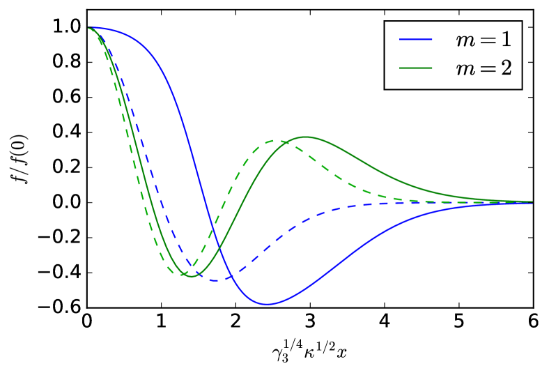
Figure 1: Solutions with $m=1$ and $2$ in the chiral limit $w=0$. The parameters are $\gamma_{2}=5000$, $\gamma_{3}=100$, $q=0.1$ and $\alpha=10^{-2}$. Dashed lines show the corresponding solutions in the small condensate approximation for $\sqrt{\gamma_{3}}/(4\kappa)\gg 1$, see Eq. (21). Under this assumption, $f/f(0)$ is, for each value of $m$, a universal function of the rescaled coordinate $\gamma_{3}^{1/4}\kappa^{1/2}x$ here used. Although the qualitative behavior of the solution is well captured by the perturbative approximation, the actual behavior requires the full numerical solution. One can also check that the behavior close to the string core ($r\to 0$) corresponds to the expected $1-f/f(0)\propto r^{2}$

3 Numerical results

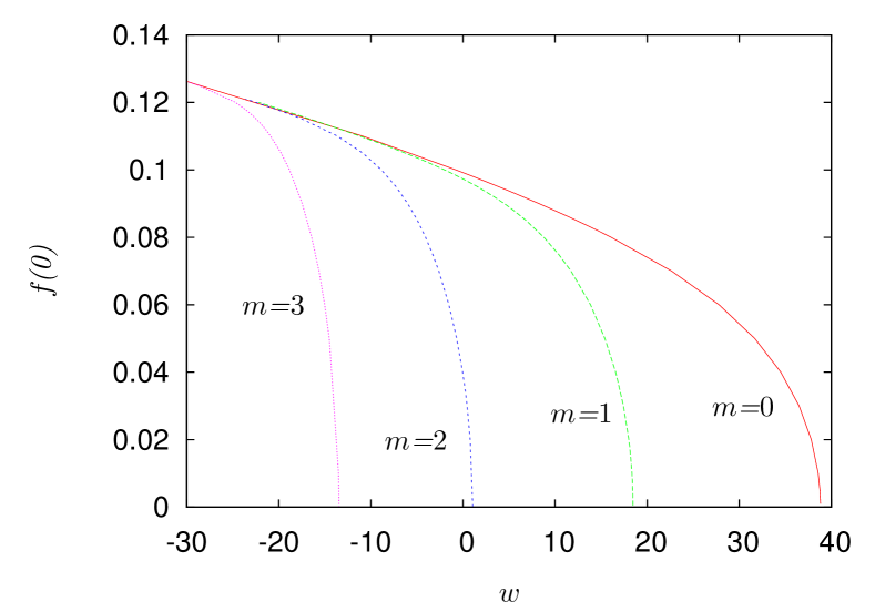
Figure 2: Value $f(0)$ of the condensate function along the string axis as a function of the state parameter $w$ for excited state numbers $m=0,1,2,3$ and the same parameters as in Fig. 1.

We have solved numerically the set of coupled non-linear differential equations (7), (8), and (9), subject to the appropriate boundary conditions (10) using an iterative Newton-Raphson/collocation method with automatic grid selection [35]. The relative errors of our solutions are typically of the order of $10^{-7}$ to $10^{-10}$. We have studied a large number of parameter values, $\alpha\in[10^{-3},10^{-1}]$, $\gamma_{i}\in[1,10^{3}]$, $i=2,3$ and $q\in]0,1]$, but report only on one specific case that is generic enough and displays the main qualitative features. The choice was made in order to fulfill the necessary constraints (see e.g. [26]) by a large margin and to allow the existence of solutions in the chiral limit $w=0$. The chiral solutions with $m=1,2$ nodes for our choice of parameters are shown in Fig. 1, together with the approximate perturbative solutions. The constant $\kappa:=h^{\prime}|_{x=0}$ is extracted from the numerical data. Our numerical results show that for this choice of parameters chiral solutions can only possess up to 2 nodes, i.e., $m\leq 2$. This is shown in Fig. 2, where we give the value of $f(0)$ as function of the state parameter $w$. This shows that, while for node number $m=0,1,2$ electric, magnetic as well as chiral solutions exist, $m=3$ solutions are always electric.

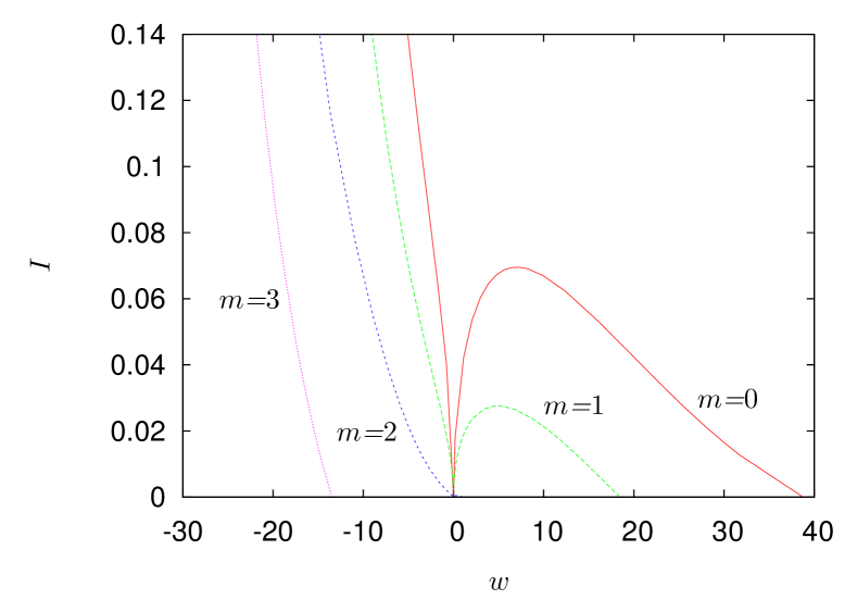
Figure 3: Current $I$ as a function of the state parameter $w$ and the same parameters as in Fig. 1.

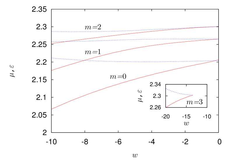
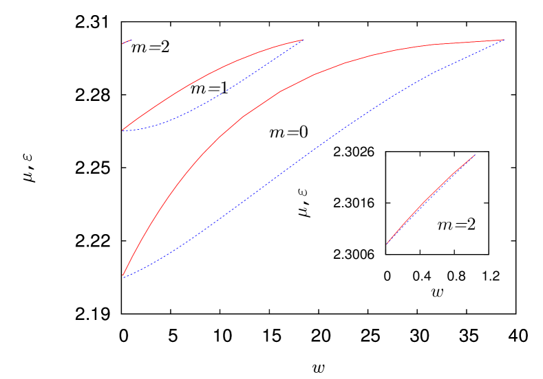
Figure 4: Energy per unit length $\varepsilon$ (red solid) and tension $\mu$ (blue dashed) as functions of the state parameter $w$ and for the same parameters as in Fig. 1 in the electric regime (top) and in the magnetic regime (bottom), respectively.

Fig. 3 displays the current $I$ of the superconducting string. We observe that the maximal possible current on the string in the magnetic regime decreases with increasing node number. In Fig. 4, we show the energy per unit length $\varepsilon$ as well as the tension $\mu$ of the strings. The qualitative behaviour of these quantities is similar in all cases.

Carter devised a macroscopic stability criterion [36] stating that a necessary condition for stability of superconducting strings is that the velocities of longitudinal (L), $c_{{}_{\mathrm{L}}}$, and transverse (T) perturbations, $c_{{}_{\mathrm{T}}}$, given by

$$c_{{}_{\mathrm{L}}}=\sqrt{-\frac{\mbox{d}\mu}{\mbox{d}\varepsilon}},\ \ c_{{}_{\mathrm{T}}}=\sqrt{\frac{\mu}{\varepsilon}},$$ (22)

respectively, should be real for the string to be stable. This occurs for the state parameter less than a limiting value (in general different for each series of solutions) which we denote by $w_{\mathrm{Carter}}$. As can be seen from Fig. 4, in our example we have $w_{\textrm{Carter}}\approx-4$ for $m=0$, and $w_{\textrm{Carter}}\approx-9$ for $m=1,2$. We expect that $w$ can become positive for a different choice of parameters, as demonstrated for $m=0$ in [23].

This criterion being a necessary condition, it permits to restrict the range of parameters in which stable solutions may exist, but doesn’t guarantee stability, even to linear order: they may support unstable modes not captured by this macroscopic criterion. Determining the presence or absence of such modes requires linearizing the field equations from the Lagrangian (1). A full linear stability analysis is beyond the scope of the present letter and will be presented in [33]. Here we exemplify the point by focusing on perturbations of $f$ only, keeping the other fields fixed. 

Inserting $f(x)=f_{0}+\delta f$, where $f_{0}(x)$ is a solution to the full set of equations (7), (8), (9) and $\delta f(x)$ is real and small, we find that (9) becomes – neglecting terms of order $(\delta f)^{2}$ and higher – a Schrödinger-type equation for $\delta f$ with potential $V_{\textrm{eff}}(x)=w+3\gamma_{2}f_{0}^{2}-\gamma_{2}q^{2}+\gamma_{3}h_{0}^{2}$, where $h_{0}(x)$ is a solution to (7), (8), (9). We find that for the solutions plotted in Fig. 1, this potential is strictly positive for the fundamental solution, but becomes negative in some range of the coordinate $x$ for the excited solutions for $w\leq 0$. This indicates a possible instability. Solving numerically the time-dependent equation on $\delta f$, we found that an unstable mode indeed exists. This is illustrated in Fig. 5, showing $V_{\textrm{eff}}$ for the fundamental and the two excited solutions computed in the small-condensate limit as well as the corresponding unstable modes. Since an instability already shows up in this linearized model, one should envisage that most of the excited solutions may be unstable. The question remains to what extent this is a generic (parameter-dependent) statement. Moreover, in the magnetic regime for which $w>0$, there must exist a threshold $w_{\mathrm{th}}$ above which the potential becomes positive definite again. The relevant solutions may then be stable provided $w_{\mathrm{th}}$ is below $w_{\mathrm{Carter}}$ defined above.

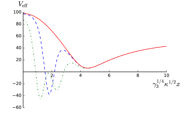
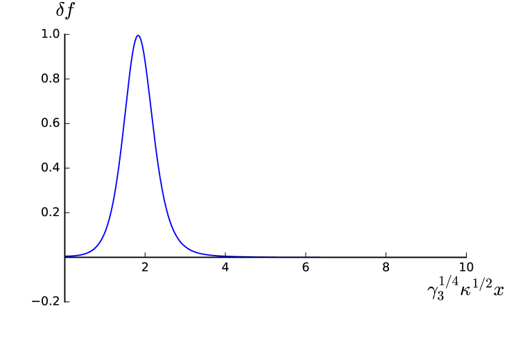
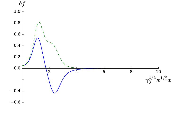
Figure 5: Top panel: Effective potential $V_{\textrm{eff}}$ for the solutions with $m=0$ (red, continuous), $m=1$ (blue, dashed), and $m=2$ (green, dot-dashed) in the small-condensate limit. The profile of $h$ is a hyperbolic tangent with parameters chosen to match those of the numerical solution with $m=0$. Middle panel: profile of the unstable mode for the solution with $m=1$. (The normalization is arbitrary.) Bottom panel: profiles of the two unstable modes for the solution with $m=2$.

4 Discussion

The above strings are of the purely spatially local type as far as the current is concerned, and this may, in some GUT-based models for instance, be considered unlikely, as most symmetries then are expected to be gauged. Indeed, many superconducting cosmic string models consider actual electromagnetic currents, and may even be used to produce large-scale primordial magnetic fields. The excited states found here are based on an uncoupled model, but we have constructed the corresponding solutions in the case where $\sigma$ is given a gauge coupling too, i.e. for $e_{\sigma}\not=0$, and found that the basic features are left unchanged [33]. Besides, as discussed in Ref. [37], the influence of such an extra coupling is expected to be mostly negligible on the microstructure and we confirmed this expectation for the excited solutions. On the other hand, such a coupling could source a different external field, leading to a more complicated large scale magnetic structure; this should be considered in a cosmological context.

We would also like to remark that the main qualitative features of these solutions persist in a dynamical space-time, i.e. when coupling the matter equations to the Einstein equation. We have checked this numerically and will report on the details of our results elsewhere [33].

We find some of these solutions to fulfill the macroscopic stability criterion of Carter, which uses integrated, macroscopic quantities regardless of the details of the underlying field theoretical model. In contrast, the microscopic stability analysis of these solutions is very much model-dependent. Since the integrated quantities stem from the underlying model though, we expect that a solution that is macroscopically unstable will also be unstable when investigating the micro-physics. Our preliminary results indicate that the excited solutions may be classically unstable microscopically, so we should not expect them to be directly observable through, e.g., gravitational lensing. Besides, it would be very difficult to distinguish an excited from a standard cosmic string through the deficit angle alone. On the other hand, the fact that these solutions are unstable may offer a possibility to detect them through particle emission during the collision and recombination of two strings. For instance, the large fluctuations of the fields during the collision may locally excite the condensate, producing a solution with $m\neq 0$ along a segment of one or both strings, the sharp transition regions between the parts with $m=0$ and $m\neq 0$ producing a current kink propagating along the string axis. Since the solutions with $m\neq 0$ are unstable, they will locally decay to the fundamental one, emitting high-energy particles. One can thus expect radiation with high energy to be emitted along a one-dimensional region of space, following the trajectory of the kink. In return, this emission should reduce the average velocity of the string network, transforming its kinetic energy into massive particle radiation.

Interestingly, the excited solutions may have close analogues in Bose-Einstein condensates, which would open possible paths to observations in laboratory experiments. It is now well known [1] that rotating condensates develop vortex lines akin to cosmic strings. Let us consider a cold gas made of two different atoms, or a single species of atoms with two internal states coupling differently to some external electromagnetic fields creating the confining potential. In principle, the potentials experienced by the two types of atoms can be tuned so that only one type of atoms condenses in the lowest-energy state, while the other type can condense inside a vortex core. The vortex could then support a supercurrent, exactly like the strings considered in this letter. Moreover, from the similarity between (7) and the stationary Gross-Pitaevskii equation, one can expect to find the same structure of solutions, with one fundamental configuration minimizing the energy and, depending on the parameters, a set of excited ones with a more complicate structure for the condensate of the second type of atoms. (This will be true generically provided the potential experienced by the second type of atoms is quadratic close to the vortex line.) To the best of our knowledge, the question of whether such a setup is possible or not is still pending.

References

- [1] A. Fetter and A. Svidzinsky, J. Phys.: Condens. Matter 13, R135 (2001).
- [2] A. A. Abrikosov, Journal of Physics and Chemistry of Solids 2, 199 (1957).
- [3] J. F. Annett, “Superconductivity, Superfluids and Condensates”, Oxford University Press (2004); A. L. Fetter, Rev. Mod. Phys. 81, 647 (2009).
- [4] M. Shifman and A. Yung, “Supersymmetric solitons”, Cambridge University Press (2009).
- [5] M. B. Hindmarsh and T. W. B. Kibble, Rept. Prog. Phys. 58, 477 (1995); See also A. Vilenkin and E. P. S. Shellard, “Cosmic Strings and Other Topological Defects,” Cambridge University Press (2000).
- [6] P. A. R. Ade et al. [Planck Collaboration], Astron. Astrophys. 571, A25 (2014).
- [7] T. Vachaspati, L. Pogosian and D. Steer, Scholarpedia 10 (2015) no.2, 31682, [arXiv:1506.04039 [astro-ph.CO]].
- [8] E. Allys, JCAP 1604, 009 (2016); Phys. Rev. D 93, 105021 (2016).
- [9] H. Nielsen and P. Olesen, Nucl. Phys. B 61, 45 (1973); (Reprinted in Rebbi, C. (ed.), Soliani, G. (ed.): Solitons and Particles, 365-381).
- [10] H. J. Vega abd F. A. Schaposnik, Phys. Rev. D 14, 1100 (1976).
- [11] D. Garfinkle and P. Laguna, Phys. Rev. D 39, 1552 (1989).
- [12] P. Laguna and P. Matzner, Phys. Rev. D 36, 3663 (1987).
- [13] D. Garfinkle, Phys. Rev. D 32, 1323 (1985).
- [14] B. Linet, Phys. Lett. A 124, 240 (1987).
- [15] A. Comtet and G. Gibbons, Nucl. Phys. B 299, 719 (1988).
- [16] M. Christensen, A.L. Larsen and Y. Verbin, Phys. Rev. D 60, 125012 (1999).
- [17] Y. Brihaye and M. Lubo, Phys. Rev. D 62, 085004 (2000).
- [18] E. B. Bogomolny, Sov. J. Nucl. Phys. 24 449 (1976); (Reprinted in Rebbi, C. (ed.), Soliani, G. (ed.): Solitons and Particles, 389-394).
- [19] A. C. Davis and P. Peter, Phys. Lett. B 358, 197 (1995).
- [20] E. Witten, Phys. Lett. B 153, 243 (1985).
- [21] B. Carter and P. Peter, Phys. Lett. B 466, 41 (1999).
- [22] C. Ringeval, Phys. Rev. D63 063508 (2001); Phys. Rev. D64, 123505 (2001).
- [23] P. Peter, Phys. Rev. D 45 1091 (1992).
- [24] P. Peter, Phys. Rev. D 46 3322 (1992).
- [25] B. Carter and P. Peter, Phys. Rev. D 52, 1744 (1995).
- [26] B. Hartmann and B. Carter, Phys. Rev. D 77, 103516 (2008).
- [27] E. Abraham, Nucl. Phys. B 399 197 (1993).
- [28] P. Forgacs, S. Reuillon and M. S. Volkov, Nucl. Phys. B 751, 390 (2006); Phys. Rev. Lett. 96, 041601 (2006).
- [29] J. Garaud and M. S. Volkov, Nucl. Phys. B 826, 174 (2010).
- [30] B. Kleihaus, J. Kunz and M. List, Phys. Rev. D 72, 064002 (2005).
- [31] P. Breitenlohner, P. Forgacs and D. Maison, Nucl. Phys. B 383, 357 (1992); Nucl. Phys. B 442, 126 (1995); P. Peter and E. Huguet, Astropart. Phys. 12, 277 (2000).
- [32] E. Babaev and J. M. Speight, Phys. Rev. B 72, 180502 (2005); P. Forgács and Á. Lukács, Phys. Rev. D94, 125018 (2016); Phys. Lett. B 762, 271 (2016).
- [33] B. Hartmann, F. Michel and P. Peter, in preparation.
- [34] M. Abramowitz, I. A. Stegun and I. Ann, Handbook of Mathematical Functions with Formulas, Graphs, and Mathematical Tables, Applied Mathematics Series 55, Washington D.C., USA (1972).
- [35] U. Ascher, J. Christiansen and R. D. Russell, Math. Comput. 33 (1979), 659; ACM Trans. Math. Softw. 7, 209 (1981).
- [36] B. Carter, Phys. Lett.B 228 466 (1989).
- [37] P. Peter, Phys. Rev. D 46, 3335 (1992).
- [38] R. L. Davis and E. P. S. Shellard, Nucl. Phys. B 323, 209 (1989); R. H. Brandenberger, B. Carter, A. C. Davis and M. Trodden, Phys. Rev. D 54, 6059 (1996).