Cellular Legendrian contact homology for surfaces, part I
Abstract.
We give a computation of the Legendrian contact homology (LCH) DGA for an arbitrary generic Legendrian surface in the -jet space of a surface. As input we require a suitable cellular decomposition of the base projection of . A collection of generators is associated to each cell, and the differential is given by explicit matrix formulas. In the present article, we prove that the equivalence class of this cellular DGA does not depend on the choice of decomposition, and in the sequel [35] we use this result to show that the cellular DGA is equivalent to the usual Legendrian contact homology DGA defined via holomorphic curves. Extensions are made to allow Legendrians with non-generic cone-point singularities. We apply our approach to compute the LCH DGA for several examples including an infinite family, and to give general formulas for DGAs of front spinnings allowing for the axis of symmetry to intersect .
1. Introduction
The Legendrian contact homology (abbrv. LCH) algebra of a Legendrian submanifold, , in the -jet space, , of a manifold is a differential graded algebra (abbrv. DGA) with generators determined by the double points of the Lagrangian projection of and with differential defined via counts of suitable spaces of pseudo-holomorphic disks. The LCH algebra was outlined in a more general setting as part of the wider class of symplectic field theory invariants in [22] and, for Legendrian submanifolds in -jet spaces, was first rigorously constructed in [14, 17].
Aside from being able to distinguish Legendrian isotopy classes, the LCH algebra is useful in identifying the border between symplectic flexibility and rigidity. For example, the existence of an augmentation of the LCH algebra of a displaceable Legendrian implies that satisfies the Arnold conjecture for exact Lagrangian immersions–roughly speaking, the projection of to must have enough double points to generate half of the homology of [16, 12]. In contrast, Legendrian submanifolds whose LCH algebras have vanishing homology have been constructed to have only double point [11]. A sample of other applications of LCH algebras include (i) surgery exact triangles explaining the effect of Legendrian surgery/symplectic handle attachment on the symplectic and contact homology of Stein manifolds and their contact boundaries [2]; (ii) a complete invariant for smooth knots in [32, 13, 25, 20] (iii) connections between the LCH algebra of -dimensional Legendrian knots and topological invariants of knots such as the Kauffman and HOMFLY polynomial [34, 29]; (iv) results concerning Lagrangian cobordisms in symplectizations [18, 8, 4].
For -dimensional Legendrians (in a -jet space), the LCH algebra is combinatorially computable, as the pseudo-holomorphic disks used to define the differential may be identified using the Riemann mapping theorem [5]. Moreover, after placing the front diagram of into a standard form, the count of such disks can be carried out in an algorithmic manner [31]. As a result, the LCH algebra is an effective tool for distinguishing Legendrian knots with reasonably sized diagrams, and is useful in distinguishing many pairs of Legendrian knots in the current tables.
In contrast, the explicit computation of Legendrian contact homology for higher dimensional Legendrians is much more challenging as direct counts of the relevant moduli of pseudo-holomorphic disks are not feasible. For Legendrians in -jet spaces, a major step towards explicit computation was carried out in [10] where it was shown that the count of pseudo-holomorphic disks can be replaced by a count of certain rigid gradient flow trees (abbrv. GFTs). This replaces the need to identify pseudo-holomorphic disks with a problem phrased entirely in terms of ODEs. However, GFTs are themselves complicated global objects. Consequently, explicit computations of the full DGA have been limited to several restricted classes of 2-dimensional Legendrians: conormal lifts of smooth knots in [13]; two-sheeted Legendrians surfaces [7]; and Legendrian tori constructed from -dimensional Legendrian knots via front and isotopy spinnings [19]. There have also been a number of partial DGA computations in higher dimensions: front spinning [15, 9]; and DGA maps induced from Lagrangian cobordims [8, 30].
In this paper and its companion [35], we give a computation of the LCH algebra with -coefficients for all -dimensional Legendrians in the -jet space of a surface. For a surface and a Legendrian , we define a cellular DGA, , that requires as input a suitable polygonal decomposition of the base projection (to ) of . To each -, -, and -cell in the decomposition we associate a collection of generators with the precise number of generators determined by the appearance of the front projection of above the cell. After placing the generators associated to a particular cell and its boundary cells into matrices, the differential of is characterized by explicit formulas. See Figure 4 for a brief summary.
The standard notion of equivalence used when considering Legendrian contact homology DGAs is known as stable tame isomorphism. This is at least as strong as the notion of homotopy equivalence for DGAs. Our main result is:
Theorem 1.1.
For any -dimensional , the cellular DGA is equivalent to the Legendrian contact homology DGA of with coefficients in . In particular, up to stable tame isomorphism, does not depend on the choice of polygonal decomposition, and is a Legendrian isotopy invariant.
In the present article, we define the cellular DGA, and prove independence of the choice of polygonal decomposition. In [35], we construct a stable tame isomorphism between the Legendrian contact homology DGA of and the cellular DGA of obtained from a particular choice of polygonal decomposition. Here, we use the reformulation of the differential in terms of GFTs [10]. We produce relatively explicit coordinate models for Legendrian surfaces to make our computations of LCH.
The differential in the cellular DGA is local in the sense that it preserves sub-algebras corresponding to generators associated to the closure of any particular cell. Starting with the splash construction [23], similar localization techniques have been developed in the case of -dimensional Legendrians where they have been applied to study augmentations of the LCH algebra and to relate the LCH algebra with invariants defined via the techniques of generating families and constructible sheaves [24, 38, 33]. The localizing splash construction has since been generalized to higher dimensional Legendrians [26, 30]. We expect that the cellular DGA may also provide an approach for extending the other applications to the -dimensional case. In particular, in the upcoming article [36] we apply Theorem 1.1 to give a necessary and sufficient condition for the existence of augmentations in terms of a -dimensional generalization of the Morse Complex Sequences studied in [28], which exists in the presence of a generating family for the Legendrian.
Although the number of generators of can be quite large, it is often possible to reduce the number of generators to a much smaller size while retaining an explicit formula for the differential. The idea is to cancel generators in pairs via a suitable stable tame isomorphisms. Throughout Section 5, we illustrate this process with explicit examples. In that section we also show how to the relax conditions on the cell decomposition (for example, allowing cone points which arise naturally in [13, 7]), which further reduces the set of generators. See Sections 5.3 and 5.4.
In Section 2, we recall background material on DGAs and Legendrian surfaces in -jet spaces. The definition of the cellular DGA is given in Section 3, where it is verified that differential has degree and satisfies ; see Theorem 3.2. Theorem 4.1 of Section 4 shows that for any fixed Legendrian , the stable tame isomorphism type of the cellular DGA is independent of the choice of polygonal decomposition and of other auxiliary choices. In Section 5.1 and 5.2, we compute the LCH of two Legendrian spheres. In Section 5.5 we compute the LCH for front-spun knots, expressing it as a natural DGA operation. Some of these computations agree with pre-existing ones. In Section 5.6, we provide a family of spheres many of which have identical Linearized homology groups, but are distinguished by product operations that would be difficult to identify without explicit formulas for differentials.
We remark that knowledge of LCH is neither assumed nor required in the current article. The required background on LCH and GFTs is postponed until [35].
2. Background
2.1. Differential graded algebras
In this article, we consider Differential Graded Algebras (abbrv. DGAs) with -coefficients and -grading for some non-negative, integer . The differential of a DGA has degree and satisfies the Liebniz rule .
A based DGA is a DGA with a chosen subset such that is freely generated by , as an associative (non-commutative) -algebra with identity. That is, so that elements of can be written uniquely as -linear combinations of words in the elements of . Furthermore, we require that the generating set consists of homogeneous elements, so that the -grading, , is determined by the assignment of degrees to generators, , and the requirement that when and are homogeneous elements.
We say that the differential is triangular with respect to a total ordering of the generating set given by if for all , where and denotes the subalgebra generated by .
2.1.1. Stable tame isomorphism
An elementary automorphism of is a graded algebra map such that for some , we have when , and where belongs to the subalgebra generated by . A tame isomorphism between based DGAs is an isomorphism of DGAs , i.e. a graded algebra isomorphism satisfying , that is a composition of elementary automorphisms of followed by an isomorphism that extends some bijection of generating sets .
The degree stabilization of a based DGA, , with generating set, , is the based DGA, , with generating set, , where the new generators are assigned degrees , , and satisfies
Definition 2.1.
Two based DGAs are stable tame isomorphic if after stabilizing each of the DGAs some (possibly different) number of times they become isomorphic by a tame isomorphism.
It can be checked that stable tame isomorphism satisfies the properties of an equivalence relation. We occasionally say that two based DGAs are equivalent to mean that they are stable tame isomorphic.
The following theorem will serve as our primary method for producing stable tame isomorphisms.
Theorem 2.1.
Let be a based DGA such that is triangular with respect to the ordered generating set . Suppose that
| where , |
and let denote the -sided ideal generated by and . Then, is free and triangular with respect to the ordered generating set . Moreover, with these generating sets, and are stable tame isomorphic.
Typically we use the same notation for an element of and its equivalence class in a quotient of . Note that to write the differential in in terms of the generating set, , we simply replace all occurrences of (resp. ) in by (resp. by ).
Proof.
This is essentially due to [5, Section 8.4].
If necessary, we can reorder as to arrange that and are consecutive while preserving the triangular property of . Thus, we can suppose with , and show is stable tame isomorphic to where . It is clear that is indeed freely generated by since we have the vector space decomposition, where is the subalgebra generated by . We next need the following.
Lemma 2.1.
There exists a DGA map such that for any , (), with .
Proof.
The projection is a DGA map. We will construct to be a homotopy inverse to .
Note that inherits a filtration from , where is the sub-algebra generated by . In particular, are all freely generated by with . Begin by defining , and on generators by
Then, extend as an algebra homomorphism, and extend to be a -derivation, meaning that . A direct verification shows that
hold when applied to generators of and , respectively. This implies that the identities in fact hold on all of and . [In general, if are DGA maps, and is a -derivation, then holds if and only if it holds on a generating set for .]
Now, for , we inductively define maps and to satisfy
-
(1)
is a chain map,
-
(2)
is a -derivation, and
-
(3)
.
Supposing and have been defined, we extend them to maps and . Begin by setting
Note that , since is triangular. Thus, this definition makes sense, and we indeed have with . Next, extend as an algebra homomorphism, put , and then extend to as a -derivation. We check that and again satisfy (1)-(3). Note that (2) holds by construction. Once (1) is known, (3) follows from the definition of since the identity holds when applied to generators of .
To verify (1), compute:
where at the second equality we used that since is triangular.
Thus, the construction proceeds inductively with satisfying the stated requirements of the Lemma. ∎
We now construct a stable tame isomorphism. Denote the generators of the stabilization, , as where, for , , and and are the two new generators from stabilization with ; the degree of the stabilization is chosen so that and . Define an algebra map by
is a chain map: It suffices to verify that holds when applied to generators. Compute
For , , so we have
is a tame isomorphism: Note that for all , where . Thus, we can write
where and .
∎
Remark 2.2.
-
(i)
The notion of stable tame isomorphism appears in [5] and is now prevalent in the literature surrounding Legendrian contact homology.
-
(ii)
A variation on stable tame isomorphism arises from requiring that the word that appears in in the definition of elementary isomorphism belongs to with respect to some ordering of generators for which is triangular. We do not know whether the equivalence on based algebras generated by such isomorphisms is distinct from stable tame isomorphism. However, we note in passing that the proof of Theorem 4.1 shows that the DGAs corresponding to distinct compatible cell decompositions of are related by this stronger equivalence.
2.2. Legendrian surfaces
Let be a surface. The -jet space, , has a standard contact structure given by the kernel of the contact form where is the Louiville -form on and is the coordinate on the factor. Any choice of local coordinates on leads to coordinates on with respect to which the contact form appears as
We denote by
the projections which are known respectively as the front projection and base projection.
A surface is Legendrian if . The singularities of front and base projections of Legendrian submanifolds are well studied, cf. [1]. In this -dimensional setting, after possibly perturbing by a small Legendrian isotopy, we may assume that such that is an embedded -manifold and is a discrete set; near each the front projection has the following standard forms.
-
•
Any has a neighborhood, , whose front projection is the graph of a smooth function defined on a neighborhood of , i.e.
In particular, the restriction of to is an immersion. We often refer to connected subsets of and/or their front projections as sheets of .
-
•
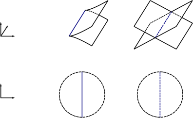
Any point in has a neighborhood whose front projection is diffeomorphic to a standard cusp edge, i.e. a semi-cubical cusp crossed with an interval, see Figure 1. Locally cusp edges belong to the closure of two sheets of that we refer to as the upper and lower sheets of the cusp edge.
-
•
Any point in has a neighborhood whose front projection is diffeomorphic to a standard swallow tail singularity. In fact, there are two types of swallow tail singularities that we refer to as upward and downward swallow tails. The Legendrian, , in defined by the generating family,
has a standard upward swallow tail singularity when . The front projection of is given by
The standard downward swallow tail singularity is obtained by negating the -coordinate. See [1, p. 47].
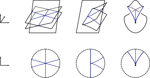
A swallow tail point, , lies in the closure of two cusp edges of ; the base projections of these two cusp edges form a semi-cubical cusp curve in with the cusp point at . The two cusp edges that meet at a swallowtail point have either their upper or lower sheet in common. (The other two sheets associated with these cusp edges meet at the crossing arc that terminates at .) When the swallowtail is upward (resp. downward) the common sheet appears above (resp. below) the two sheets that cross in the front projection.
As long as is an embedded Legendrian, the front projection of must be transverse to itself. [Since the and coordinates are recovered by .] Again, after a small perturbation, we can assume is also transverse to and as well as to the self intersection set of to arrange that the self intersections of are as follows:
-
•
Along crossing arcs two sheets of intersect transversally.
-
•
At isolated triple points three sheets of meet in a manner that is pairwise transverse, and so that the crossing arc between any two of the sheets is transverse to the third sheet. In the base projection, three crossing arcs meet at a single point, but are pairwise transverse.
-
•
At isolated points, , a cusp-sheet intersection occurs where a cusp edge cuts transversally through a sheet of . The crossing arcs between this sheet and the upper and lower sheets of the cusp edge both end at . The base projections of these two crossing arcs meet at a semi-cubical cusp point on the base projection of the cusp edge.
We refer to the union of the crossing arcs, cusp edges, and swallowtail points in either the front or base projection (depending on context) as the singular set of . We denote the base projection of the singular set as . When has generic base projection, we write
where points in are in the image of a single crossing are or cusp edge, and is a finite set containing the image of codimension parts of the front projection as well as points in the transverse intersection of the image of two distinct cusp edges and/or crossing arcs. Often, we will refer to the base projections of cusp edges, and crossing arcs as the cusp locus and the crossing locus. See Figures 1 and 2 for the local appearance of the singular set.
[l] at 38 48 \pinlabel [b] at 2 86 \pinlabel [l] at 38 200 \pinlabel [l] at 22 226 \pinlabel [b] at 2 238 \pinlabelCusp Edge [t] at 202 -4 \pinlabelCrossing Arc [t] at 394 -4 \endlabellist
[l] at 38 48 \pinlabel [b] at 2 86 \pinlabel [l] at 38 200 \pinlabel [l] at 22 226 \pinlabel [b] at 2 238 \pinlabelTriple Point [t] at 178 -4 \pinlabelCusp-Sheet Intersection [t] at 354 -4 \pinlabelSwallow Tail [t] at 530 -4 \endlabellist
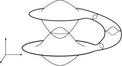
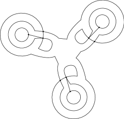
Conversely, any surface in matching the above description and without vertical tangent planes is the front projection of a unique Legendrian . See Figure 3 for an example of a Legendrian surface in pictured in its front and base projection.
2.2.1. Maslov potentials
A generic loop in is disjoint from swallowtail points and crosses cusp edges transversally. Let where (resp. ) is the number of points where crosses from the upper to lower sheet (resp. lower to upper sheet) at a cusp edge. The (minimal) Maslov number for , is the smallest positive integer value taken by , or if all loops have .
A Maslov potential is a locally constant function
whose value increases by when passing from the lower sheet to the upper sheet at a cusp edge. When is connected, any two Maslov potentials differ by the overall addition of a constant.
3. Definition of the cellular DGA
In this section we associate a DGA to a Legendrian surface, , using an appropriately chosen cell decomposition of . Initially we assume that the front projection of does not contain any swallowtail singularities as this simplifies the definition. In Sections 3.7-3.13, we complete the definition by addressing the case when swallowtail points are present.
3.1. Compatible cell decompositions
Let be a surface. By a polygonal decomposition of , we mean a CW-complex decomposition of ,
with characteristic maps satisfying:
-
(i)
The characteristic maps for -cells are smooth.
-
(ii)
For any two cell , preimages of -cells divide the boundary of into intervals that are mapped homeomorphically to -cells by .
Note that we allow that the same -cell may appear multiple times in the boundary of a given -cell. Compare with the decomposition pictured in Figure 11.
Let be a Legendrian submanifold with generic front projection, and denote by the base projection of the singular set of , where and are the singularities of codimension and respectively. We say that a polygonal decomposition of is compatible with or -compatible if is contained in the -skeleton of . From the nature of codimension singularities, it follows that must be contained in the -skeleton.
[t] at 62 26 \pinlabel [tr] at -3 3 \pinlabel [r] at 12 78 \endlabellist
 \labellist\pinlabel [t] at 50 282
\pinlabel [r] at -2 240
\endlabellist
\labellist\pinlabel [t] at 50 282
\pinlabel [r] at -2 240
\endlabellist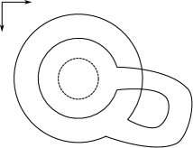
3.2. Definition of the cellular DGA
Assume that is a compatible polygonal decomposition for a Legendrian whose front projection is without swallowtail points. We now associate a differential graded algebra, , to using . We will refer to as the cellular DGA of , and in Section 3.7 we extend the definition to allow swallowtail points.
The definition of requires the following additional data associated to . For each -cell, , we choose an initial and terminal vertex from points of that are mapped to -cells by , and label these points and . We allow that , but in this case we must also declare a direction for the path around the circle from to .
3.3. The algebra
When referring to sheets of above a cell we mean those components of that are not contained in a cusp edge. We denote the set of sheets of above as where is an indexing set. The sets are partially ordered by decreasing -coordinate, and we write if above . Two sheets are incomparible if and only if they meet in a crossing arc above in the front projection of .
The algebra is the free unital associative (non-commutative) -algebra with generating set arising from the cells of as follows. For each cell we associate one generator for each pair of sheets , satisfying . We denote these generators as , , or in the case of a -cell, -cell, or -cell respectively. The superscript will sometimes be omitted from notation.
3.4. The grading on
A choice of Maslov potential, , for allows us to assign a -grading to as follows (where is the Maslov number of ). Each of the generators is a homogeneous element with degree given by
| (1) |
When is connected the grading is independent of the choice of .
3.5. Algebra in
In the remainder of the article, we often make computations in the ring, , of matrices with entries in . Any linear map extends to a linear map by applying entry-by-entry. Moreover, if is an algebra homomorphism (resp. a derivation), then the resulting extension is also an algebra homomorphism (resp. a derivation). Note that a derivation of with will annihilate any matrix of constants in , so that for instance we can compute if .
In our notation, we will use to denote a matrix with all entries except for the -entry which is .
3.6. Defining the differential
We define the differential, , by requiring ; specifying values on the generators of ; and then extending as a derivation. Generators that correspond to cells of dimension , and are considered separately in the definition.
3.6.1. -cells
For a zero cell, , extend the partial ordering to a total linear order via a bijection , so that the (non-cusp) sheets above are labeled as with . Using this ordering, we arrange the generators corresponding to into a strictly upper triangular matrix with -entry given by if and otherwise. The differential is then defined so that the matrix equation
| (2) |
holds with applied entry-by-entry.
Lemma 3.1.
There is a unique way to define so that (2) holds. Moreover, is independent of the choice of extension of to a total order, and .
Proof.
Uniqueness is clear since contains each as an entry. That such a definition is possible requires that all non-zero entries of correspond to non-zero entries of . Using for the entries of , the -entry of is where the latter sum is over those such that and hence vanishes unless . It is also clear that the sum depends only on and not the choice of extension to a total order.
To see that , compute
∎
3.6.2. -cells
For generators corresponding to a -cell, , extend to a total order via a bijection and form an matrix with . The characteristic map for allows us to refer to the -cells at the boundary of as initial and terminal vertices, and we denote these cells as and . (It may be the case that .) The values, , are determined by the matrix equation
| (3) |
where are matrices formed from the generators corresponding to in a manner that will be described presently.
For convenience of notation, we only define as the definition of is identical. Each sheet above belongs to the closure of a unique sheet of . Since we have already chosen a bijection, , this produces an order preserving injection . Those sheets of not in the image of meet in pairs at cusp points above . We form so that the entry is if and , ; the entry is if the and sheets of meet at a cusp above ; and all other entries are . Alternatively, one can think of using the total ordering arising from to form a matrix out of the and then inserting blocks of the form along the diagonal for each pair of sheets of that meet at a cusp above . For example, if there are sheets above and the top two meet at a cusp at , then .
Lemma 3.2.
There is a unique way to define so that (3) hold. Moreover, is independent of the extension of to a total order, and .
Proof.
In order to be able to define so that (3) will hold, we need to know that for any entries of , the corresponding entry of the right hand side of (3) is . This is only an issue when is in the base projection of a crossing arc as otherwise is a full strictly upper triangular matrix, and in general the matrices (resp. ) are strictly upper triangular (resp. upper triangular). Assuming the and sheets cross above , it suffices to check that is strictly upper triangular with the -entry equal to . This is clear since the sheets of that correspond to the and sheets of must also have the same -coordinate above .
To check independence of from the choice of total order, we again only need to consider the case of a crossing arc above . The two choices of total order lead to matrices and that are related by conjugation by the permutation matrix associated to the transposition of the two sheets that cross. The corresponding matrices and are related in the same manner. Therefore, the equations are equivalent since
where we use the observation from Section 3.5 in the -nd equivalence.
To verify , observe that in all cases because of (2) combined with the block nature of the matrix and the computation . We compute
∎
3.6.3. -cells
For a -cell, , the partial ordering of sheets in is a total ordering, so we take for the indexing set and label sheets as with . Using this ordering of sheets above , we identify the sheets above all of the edges and vertices that appear along the boundary of with subsets of . Then, for each such edge (resp. vertex) we can place the corresponding generators (resp. ) into an matrices with blocks of the form (resp. ) inserted in the position along the diagonal whenever sheets meet at a cusp above the edge (resp. vertex).
Recall that for each -cell we have chosen initial and terminal vertices, and , along the boundary of that are mapped to -cells of via the characteristic map, , for the -cell. Let and denote paths in that proceed counter-clockwise and clockwise respectively from to . (If , then we choose one of these paths to be constant and the other to be the entire circle as mentioned in Section 3.2.) We let (resp. ) denote the matrices associated (as in the previous paragraph) to the successive edges of that appear in the image of (resp. ). In addition, we let and be the matrices associated (as in the previous paragraph) to the initial and terminal vertices and . Collecting the generators corresponding to into the strictly upper triangular matrix , we define so that
| (4) |
where the exponent, , is (resp. ) if the parametrization of the edge corresponding to given by has the same (resp. opposite) orientation as the characteristic map of the -cell. See Figure 4.
| -cell: |
\labellist\pinlabel [t] at 4 -4
\pinlabel [bl] at 2 12
\endlabellist |
|
| -cell: |
\labellist\pinlabel [b] at 4 14
\pinlabel [b] at 116 14
\pinlabel [b] at 58 18
\endlabellist |
|
| -cell: |
\labellist\pinlabel [l] at 156 40
\pinlabel [t] at 52 0
\pinlabel [l] at 198 133
\pinlabel [tr] at -3 3
\pinlabel [r] at 118 168
\pinlabel [r] at 20 76
\pinlabel [bl] at 202 184
\pinlabel [bl] at 102 84
\endlabellist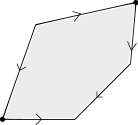
|
Lemma 3.3.
We can uniquely define so that (4) holds. Moreover, .
Proof.
First, observe that since the matrices are strictly uppertriangular, and hence nilpotent in , the inverse of is given by the finite geometric series
That the equation (4) may be obtained relies on the right hand side being strictly upper triangular. This follows since the first two terms are strictly upper triangular and the -rd and -th terms both have the form where is strictly upper triangular.
Next, each corresponds to a -cell, , in . Moreover, has initial and terminal vertices (using the orientation of to distinguish initial from terminal). Denote by and the matrices associated to these vertices using the total ordering and insertion of blocks specified by the -cell . We claim that
| (5) |
Indeed, as long as there are not two sheets of that meet at a cusp above , this is just (3) with matrices formed using the total order from . If it does happen that share a cusp edge in their closure above , then the matrix , (resp. ) is obtained from the corresponding matrix in (3) by forming a block matrix with (resp. ) inserted at the part of the diagonal of (resp. ). Then, using block matrix calculations, (5) follows from (3) and the calculation for matrices
This gives us that where the correspond to the initial and terminal vertex of with respect to the orientation given by or rather than by the orientation of itself. That is, if , and if . Since for and , the sums arising from expanding and using the Liebniz rule telescope to give
and
With these formulas in hand, follows in a straightforward manner from (4). ∎
Explicit examples computing this differential appear in Section 5.
3.7. Extending the definition to allow swallowtail points
For a Legendrian with swallowtail points and compatible polygonal decomposition , the DGA is defined in the same general manner. For a cell whose closure is disjoint from the base projections of swallowtail points, generators and differentials are defined as in Section 3.2. The appropriate modifications of the definition for -cells, -cells, and -cells that border swallow tail points are given below in 3.10, 3.12, and 3.13.
3.8. Local appearance near a swallowtail point
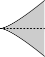
Suppose that is the base projection of a swallowtail point of . The singular locus near consists of arcs that share a common end point at . Two of these arcs are projections of cusp edges that meet in a semi-cubical cusp point at , and the third is a crossing arc that lies between the cusp arcs. See Figure 5. In a neighborhood of , we refer to the region between the two cusp arcs (right of the cusp point in Figure 5) as the swallowtail region. Note that there are more sheets above the swallowtail region than there are above its complement.
 \labellist\pinlabel [c] at 58 92
\pinlabel [c] at 58 66
\pinlabel [c] at 266 92
\pinlabel [c] at 266 66
\endlabellist
\labellist\pinlabel [c] at 58 92
\pinlabel [c] at 58 66
\pinlabel [c] at 266 92
\pinlabel [c] at 266 66
\endlabellist
Recall that the appearance of the front projection of near a swallowtail point has one of two distinct types depending on if the is an upward or downward swallow tail. We use the convention of indexing the sheets that meet at an upward (resp. downward) swallowtail point as , , (resp. , , ), so that (resp. ) denotes the upper (resp. lower) sheet and the and (resp. and ) sheets cross near . The single sheet outside the swallowtail region that contains in its closure is then labeled (resp. ).
3.9. Decorations at swallowtail points
Defining in the presence of swallowtail points requires some additional data. Within a neighborhood of each swallowtail point, , we choose a labeling of the two regions (subsets of -cells of ) that border the crossing arc that ends at ; label one of the regions with an and the other with a . See Figure 5.
3.10. -cells
In case the -cell, , is the projection of a swallowtail point the definition of the algebra does not require serious modification. Just note that we do consider the swallowtail point itself to be a sheet of so that there are the same number of generators as if were located in the complement of the swallowtail region. The differential is defined by (2) as usual.
3.11. Matrices associated to a swallowtail point
For each swallow tail point, , we will use several matrices formed from the generators, , associated to (which is necessarily a -cell of ). Near , we suppose that there are sheets above the swallow tail region, and in the complement of the swallow tail region. This is partly inspired by the swallowtail discussion of Cerf theory in [27].
The sheets above itself are totally ordered, and we let denote the matrix with non-zero entries . For , we let denote the matrix obtained from by inserting the block along the main diagonal at the (possibly non-consecutive) and rows and columns with the rest of the entries in these rows and columns equal to .
In the case of an upward swallowtail point that involves sheets and , we use the following matrix notations:
| (7) |
In the case of a downward swallowtail point that involves sheets and , we use
| (8) |
For instance, if there are -sheets above the swallow tail region of an upward swallow tail, , that involves sheets , and , then
Remark 3.1.
These somewhat mysterious matrices may be interpreted in a nice way using generating families. When is defined by a generating family, , the sheets of above correspond to the critical points of . Suppose that the entries, , of are replaced with the mod count of gradient trajectories connecting sheet to near the swallow tail point, but outside of the swallowtail region. Then, the matrices and are continuation maps determined by the collection of handleslides that end at the swallowpoint as specified in [27]. The matrices and represent the differential in the Morse complex of above a point belonging to the crossing arc that ends at the swallowtail point, with respect to the ordering of basis vectors (i.e. sheets of ) as they appear above the regions decorated with and . See [36] for more details.
Lemma 3.4.
We have
Moreover, for an upward swallowtail
| (9) |
for a downward swallowtail
| (10) |
Proof.
We verify these formulas in the case of an upward swallowtail. The case of a downward swallowtail is similar.
Compute
where the second equality follows since and . That is similar.
For the second equation of (9), we compute from definitions
To establish the first equation of (9), begin by observing that, for the permutation matrix of the transposition , we have
| (11) |
Indeed, because all entries below the row of are , and . Next, note that
| (12) |
where the second equality is due to the block in the rows of . Finally, using (11) and (12) compute
(In the -rd equality we used that and are both self inverse.)
This gives . Since , multiplying on left and right by gives . One checks that , so this completes the proof.
∎
3.12. -cells
Suppose that a -cell has its initial vertex, , or terminal vertex, , at a swallowtail point. The generators, , associated to arise from the partially ordered set of sheets as usual, and the differential is again characterized by (3). However, some adjustment may be required in forming the matrices . To simplify notation, we define in case is a swallowtail point, , and we note that an identical definition applies for if is a swallowtail point.
-
•
Suppose is outside the interior of the swallowtail region near , including if lies in either of the cusp arcs ending at . We then form the matrices and as in 3.6.2. (No issues arise as the sheets of are then totally ordered by , and the swallow tail point in is in the closure of a unique sheet of .)
-
•
Suppose is in the interior of the swallowtail region, and is not contained in the crossing arc that terminates at . Then, is totally ordered, and we form as in 3.6.2. In addition, we set
(resp. ) if is an upward (resp. downward) swallow tail point. (That is, in the upward (resp. downward) case we form as if the upper (resp. lower) of the swallowtail sheets above meet at a cusp above .)
-
•
Suppose is contained in the crossing arc that ends at the swallowtail point above . In forming the matrix, , there are two possible choices for extending the ordering of to a total order. If the total ordering used agrees with the ordering of sheets on the side of the swallow tail decorated with an , then we set
(13) If instead the ordering agrees with the side of the swallow tail decorated with a , then
(14)
Lemma 3.5.
With and formed in this manner, equation (3) leads to a well defined definition of , and .
Proof.
First, we verify well-definedness. The total ordering of is uniquely determined except in the case where is contained in a crossing locus. Suppose that this is the case and that is a swallowtail point. (When is a swallowtail point the same argument applies.) Changing the choice of total ordering conjugates by the permutation matrix, , of the transposition The corresponding definitions of from (13) and (14) are related in the same manner since
Thus, as in the proof of Lemma 3.2, the two versions of (3) that arise from different choices of ordering of are equivalent.
Since the and sheets cross above , it is also necessary to check that the entry of the right hand side of (3) is . Here, it is enough to check that is strictly upper triangular with the -entry equal to . (This implies that has the desired property, and a similar argument or the argument of Lemma 3.2 applies to the term.) Since either ordering produces an equivalent equation, we can assume that the total ordering for sheets of coincides with the order of sheets in the region. Then, we can compute the diagonal block at rows of to be
The computation goes through as before since, according to Lemma 3.4, it is still the case that . ∎
3.13. -cells
For a -cell, , the boundary of the domain of the characteristic map can be viewed as a polygon, , with edges mapping to -cells and vertices mapping to -cells of . Some vertices may have their sufficiently small neighborhoods in mapping to a region near a swallowtail point that is labeled with an or . We indicate this pictorially by placing an or near the corresponding corner of , and we form a new polygon by adding an extra edge that cuts out each such corner. Thus, the edges of each correspond to either a -cell of or an or region at a swallow tail point. Those edges corresponding to -cells receive orientations according to the orientation of the -cells (provided by characteristic maps). We orient the new and edges so that the orientation points away from the endpoint shared with the crossing arc that terminates at the swallow tail point. See Figure 6.
\labellist\pinlabel [r] at -4 113
\pinlabel [b] at 60 142
\pinlabel [l] at 21 185
\endlabellist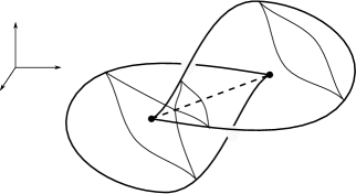
\labellist\pinlabel [t] at 112 82
\pinlabel [b] at 112 88
\pinlabel [t] at 206 82
\pinlabel [b] at 206 88
\pinlabel [c] at 156 122
\pinlabel [c] at 156 47
\pinlabel [c] at 49 128
\pinlabel [c] at 253 128
\pinlabel [r] at 66 84
\pinlabel [l] at 248 84
\pinlabel [tr] at 108 56
\pinlabel [br] at 106 113
\pinlabel [tl] at 209 58
\pinlabel [bl] at 189 129
\pinlabel [b] at 170 86
\endlabellist
\labellist\pinlabel [b] at 30 12
\pinlabel [b] at 134 12
\pinlabel [br] at 50 86
\pinlabel [bl] at 112 86
\pinlabel [t] at 96 6
\pinlabel [tr] at 232 40
\pinlabel [tl] at 378 40
\pinlabel [br] at 270 102
\pinlabel [bl] at 338 102
\pinlabel [t] at 318 6
\pinlabel at 81 54
\pinlabel at 308 54
\endlabellist
Next, we assign a matrix to each vertex of . We identify each such vertex with a -cell in by using the characteristic map of and declaring that both endpoints of and edges are identified with the swallowtail point of the corresponding or region. As before, we use the total ordering of sheets above and the nature of the singular set above to form a matrix from the generators of the -cell with the following modifications made when is a swallowtail point.
-
•
Suppose is the initial vertex of an or edge with respect to the orientation of that edge. Then, we respectively set or .
-
•
Suppose is the terminal vertex of an or edge or that small neighborhoods of are mapped within the swallow tail region, but not to one of the regions or . Then, if the swallowtail is upward , and if the swallowtail is downward . (That is, we form as if were located on the portion of the cusp edge at the swallowtail point that is in the same half of the swallow tail region as the image of a neighborhood of .)
-
•
If the -cell is in the complement of the swallowtail region, then no adjustment is required to define . (That is, .)
Next, we assign a matrix to each edge of as follows.
-
•
Suppose is an edge corresponding to a -cell of . Then, we use the total ordering of the sheets above and the nature of the singular set above to place the generators associated to into an matrix . This is precisely as in Section 3.6.3. We then set
-
•
Suppose is an edge corresponding to an region at a swallowtail point. Then, we take .
-
•
Suppose is an edge corresponding to a region. Then, we take .
We form an upper triangular matrix from the generators associated to . To define , we make a choice of an initial and terminal vertex and from the vertices of . [Once again, if , then a direction needs to be chosen for the path around from to .] We let and denote paths around that respectively proceed counter-clockwise and clockwise from to . [If , one of these paths is constant as specified by the choice of direction from to .]
Let (resp. ) denote the matrices associated to successive edges of that appear along (resp. ), and let and be the matrices associated to the vertices and . We define so that
| (15) |
where the exponent, , is (resp. ) if the orientation of the corresponding edge of agrees (resp. disagrees) with the orientation of . Here, it is useful to note that and .
Lemma 3.6.
Equation (4) leads to a well defined definition of , and .
Proof.
Equation (15) may be used to define , since the matrices and are strictly upper triangular and the are upper triangular with ’s on the diagonal. [Thus, both products have the form with strictly upper triangular, so that the entries on the main diagonal cancel.]
Recall that matrices have been assigned to all edges and vertices of . For an edge, , of let , and denote the matrices so assigned to and the initial and terminal vertices and of (with respect to the orientation of ). We claim that
| (16) |
Note that can then be checked using an argument similar to the proof of Lemma 3.3 with (16) used in place of (5). In the case where corresponds to a -cell of , (16) follows from observing the relation between the matrices and , formed when viewing and as belonging to the boundary of , and the matrices and from (3) that are used in defining the differential of the generators associated to . As in the proof of Lemma 3.3, if it is not the case that two sheets of meet at a cusp above , then and provided that, in forming and , we use the ordering of sheets above and follow the provisions of 3.12.
An explicit example computing this differential with swallowtails appears in Section 5.2.
We summarize the results of Section 3.
Theorem 3.2.
The cellular DGA satisfies . A choice of Maslov potential, , on provides a -grading on for which has degree .
Proof.
That has been verified during the definition of . Using equation (1) it is straightforward to verify that has degree . ∎
4. Independence of cell decomposition
In this section we prove the following:
Theorem 4.1.
The stable tame isomorphism type of the cellular DGA is independent of the choice of cell decomposition and additional data.
This requires showing independence of the following items:
-
(1)
The orientation of -cells.
-
(2)
The choice of initial and terminal vertex for each -cell.
-
(3)
The choice of decorations at swallow tail points.
-
(4)
The choice of cell decomposition .
These results are obtained in Corollary 4.1, Corollary 4.2, and Theorem 4.6 below. Before embarking upon their proof we collect some algebraic preliminaries.
4.1. Ordering of generators
Our main tool for producing stable tame isomorphisms will be Theorem 2.1 whose application requires a DGA to have its generating set ordered so that the differential becomes triangular. Such orderings are provided for the cellular DGA in the following Lemma 4.1.
The cellular DGA was constructed in Section 3 with a specific genererating set. Define a partial ordering of this generating set, , by declaring that if
-
(1)
The cell corresponding to has larger dimension than the cell corresponding to , or
-
(2)
The same cell, , corresponds to both and , and subscripts and for and are such that and holds in .
Lemma 4.1.
The differential of is triangular with respect to any ordering of the generating set that extends .
Proof.
As in the proof of Lemma 3.1, we have with the sum over those sheets such that . Therefore, all of these generators satisfy .
In the formula (3) that characterizes , only and give rise to terms that do not correspond to cells of lower dimension. Recall that a total ordering is used to form the matrices and , so that the term corresponds to a sum in where . Since , unless the sheets and are incomparible in . However, if this is the case then the entry was checked to be in Lemma 3.2 and Lemma 3.6. The term is handled similarly.
For a generator corresponding to a -cell, only the terms and are relevant. Since the sheets above a -cell are totally ordered, we have for . ∎
4.2. Elementary modifications to a compatible polygonal decomposition
To prove Theorem 4.1, we begin by showing that the stable tame isomorphism type of is invariant under certain local changes to the defining data.
4.2.1. Subdividing a -cell
We say that compatible cell decompositions and for are related by subdividing a -cell if is obtained from by dividing a -cell, , into two pieces, and , by placing a new vertex somewhere along . Let and denote the endpoints of in that become endpoints of and respectively in . See Figure 7 (a).
[b] at 60 86 \pinlabel [b] at 248 86 \pinlabel [b] at 302 86 \pinlabel [t] at 3 76 \pinlabel [t] at 116 76 \pinlabel [t] at 220 76 \pinlabel [t] at 276 76 \pinlabel [t] at 332 76 \pinlabel [c] at -26 76 \pinlabel [c] at -26 8 \pinlabel [c] at 136 8 \pinlabel [c] at 288 8 \endlabellist

Theorem 4.2.
Suppose that and are related by subdividing a -cell. Moreover assume that:
-
(1)
The orientation of agrees with the orientation of .
-
(2)
The and regions at swallow tail points, as well as initial and terminal vertices for -cells of and are chosen in an identical way.
Then, the corresponding cellular DGAs are stable tame isomorphic.
Proof.
Let and denote the DGAs associated to and respectively. We fix a total ordering of the sheets in , and use this choice to produce total orderings of and . We can then collect corresponding generators of (resp. ) into matrices (resp. ) where, in the case that or is a swallow tail point, we follow the instructions from 3.12 when forming or .
Assume the orientation of is from to , as the argument for the reverse orientation is similar. Then, we have
and
We can extend the partial ordering, , to a total ordering so that all of the generators corresponding to are greater than the generators corresponding to . Working in increasing order of the , we then apply Theorem 2.1 inductively to cancel the generators in pairs with the . [Note that the sheets above are in bijection with the sheets of and have the same partial ordering. Therefore, the generators and are in bijective correspondence.] In the resulting quotient, the entries of will all be replaced by the corresponding entries of . This is because of the order that we cancel the ; at the inductive step, any of the terms that would appear in have already been cancelled, and we indeed have where is the corresponding entry in (which is less than as required in Theorem 2.1).
Thus, the resulting stable tame isomorphic quotient is obtained from by replacing with , and replacing all occurrences of in with . [Note that this includes in if is a -cell bordering . When compared with there is an extra factor in corresponding to the edge . This term is replaced with in the quotient.]
∎
Corollary 4.1.
The stable tame isomorphism type of is independent of the orientation of -cells of .
4.2.2. Subdividing a -cell
Suppose that and are cell decompositions of that are compatible with and that is obtained from by removing a -cell, , that borders two distinct -cells, and , of . Thus, has a single -cell, , satisfying
Note that (because is compatible with ) it is necessarily the case that is disjoint from . We say that and are related by subdividing a -cell of . See Figure 8.
Theorem 4.3.
Suppose and are related by subdividing a -cell. Suppose in addition that:
-
(1)
Initial and terminal vertices are chosen for -cells of and so that the initial and terminal vertices of are chosen to coincide with those of , and the choice made for all remaining -cells of coincides with the choice for the corresponding -cells of .
-
(2)
The and sides of the crossing locus are assigned near each swallowtail point in an identical manner for and . Here, we allow for the possibility that borders and regions at either of its endpoints.
Then, the associated cellular DGAs are stable tame isomorphic.
Proof.
As in Section 3.13, let , , and denote the polygons associated to the -cells , of and the -cell respectively. In addition, for , let denote the paths around from the initial vertex to the terminal vertex. Note that the edge appears precisely once along either or and once along either or . Since interchanging the notations of and has no effect on the definition of the differential from (15), we can assume without loss of generality that and each contain exactly once. Moreover, in view of Corollary 4.1 we may assume that the orientation of agrees with the orientation of . Using for concatenation of paths, we can then write
where and some of these paths may be constant. Note that
| (17) |
See Figure 8.
[c] at 132 132 \pinlabel [c] at 308 124 \pinlabel [c] at 722 132 \pinlabel [l] at 230 132 \pinlabel [tr] at -2 122 \pinlabel [t] at 90 2 \pinlabel [b] at 98 264 \pinlabel [t] at 162 8 \pinlabel [bl] at 170 236 \pinlabel [bl] at 390 224 \pinlabel [tl] at 390 44 \pinlabel [l] at 404 138 \pinlabel [br] at 306 216 \pinlabel [t] at 306 28 \pinlabel [t] at 824 28 \pinlabel [tr] at 544 122 \pinlabel [b] at 634 264 \pinlabel [t] at 626 2

In view of Corollary 4.1, we may assume the orientation of is from the initial vertex to the terminal vertex. Using Theorem 2.1, we now show that the DGAs and are stable tame isomorphic. Collect generators of (resp. ) associated to and (resp. to ) into matrices and (resp. ). We choose an extension of the ordering of generators of from to a total order so that the generators corresponding to are larger than any other -cell generators. Using this ordering we can inductively cancel the with the using Theorem 2.1. [Indeed, expanding the product of edges along that appears in equation (15) for allows us to write
| (18) |
where the matrix is strictly upper triangular with and has its entry in the sub-algebra generated by generators from -cells and -cells different from and also those with such that at least one of the first and last inequalities is strict, i.e. those with . Therefore, we can apply Theorem 2.1 and inductively quotient by ideals generated by and according to the increasing ordering of these generators. For the inductive step, it is important to observe that, as long as for such that , equation (18) shows that where belongs to the subalgebra generated by those with .]
The resulting quotient has the and removed from the generating set. Moreover, the relations
allow us to find
| (19) |
(We have indicated which parts of the paths and the various portions of the product correspond to. The matrices are as in Section 3.13, and some of them may be or matrices from corners decorated at swallowtail points.)
Finally, note that becomes identical to after making the substitution (19). [Compare with (17).] It follows that the identification of with provides an isomorphism between this quotient of and .
∎
Corollary 4.2.
The stable tame isomorphism type of is independent of the choices of initial and terminal vertices for -cells.
Proof.
Let be an -compatible polygonal decomposition of , and let be any -cell of . Let denote a cellular DGA formed from using and as the initial and terminal vertices for .
Pick a -cell, , appearing in the boundary of and modify the cell decomposition to by adding a loop edge, , from to itself that is contained in . This subdivides into two pieces and where is exterior to and is interior to . Choose initial and terminal vertices of to be and , and choose both initial and terminal vertices of to be . Keep all other choices the same. Then according to Theorem 4.3 the DGA associated to is stable tame isomorphic to . On the other hand, if we reverse the role of and , we see that the DGA associated to modified so that the initial and terminal vertices and for are both replaced with is also stable tame isomorphic to . Since stable tame isomorphism satisfies the properties of an equivalence relation, it follows that the stable tame isomorphism type of is independent of the choice of and . See Figure 9. ∎
[t] at 74 -2 \pinlabel [b] at 82 260 \pinlabel [t] at 384 -2 \pinlabel [b] at 402 258 \pinlabel [tl] at 534 38 \pinlabel [tl] at 854 38 \pinlabel [c] at 268 124 \pinlabel [c] at 590 124 \endlabellist

4.2.3. Deleting an edge with -valent vertex
Suppose that an edge of has an endpoint at a -valent vertex. The edge and vertex must be disjoint from the singular set , and therefore we can delete them to produce another -compatible cell decomposition of which we denote as .
Theorem 4.4.
For and related by deleting an edge with -valent vertex, the associated cellular DGAs for are stable tame isomorphic.
Proof.
Cancel the generators of the -cell with the generators of the univalent vertex as in the proof of Theorem 4.2. ∎
4.3. Independence of and decorations at swallow tail points
Theorem 4.5.
The stable tame isomorphism type of the cellular DGA is independent of the choice of and regions at swallowtail points.
Proof.
It suffices to establish stable tame isomorphism between cellular DGAs and arising from a common -compatible decomposition, , such that the choice of and regions is opposite at a single swallowtail point, , as pictured in Figure 10. We give the proof only in the case of an upward swallowtail with sheets above the swallow tail region and so that sheets and meet at the swallowtail point. The case of a downward swallowtail is similar.
Using Theorems 4.2 and 4.3 as well as Corollaries 4.1 and 4.2, we may assume that
-
•
The -cell, , that has an endpoint at and is contained in the crossing arc is oriented away from .
-
•
The -cells containing the and regions are distinct.
-
•
The initial and terminal vertices of these -cells are disjoint from , and the orientations of the paths around the boundaries of the -cells agree with the orientation of as they pass around the corner of the and regions.
Fixing an orientation of (the base surface) near the swallowtail point, we collect the generators for the -cell that sits to the left (resp. right) of into matrices and . We form a matrix from the generators for by using the total ordering of sheets as it appears to the left of , so that rows and columns of and correspond to the same sheets. The generators associated to the swallowtail point itself are placed in an matrix , and we have matrices , , , and as defined in Section 3.11. We suppose that for (resp. ), the region is to the right (resp. left) of and the region is to the left (resp. right) of . See Figure 10.
We define an algebra morphism by requiring that when applied entry by entry
| (20) |
and for any generator that is not associated to the -cell . To verify that (20) can be obtained by a unique assignment of values it is necessary to note that where is strictly upper-triangular with entry is equal to . The latter claim holds since it is true for and also for
| (21) |
We claim that is in fact a tame isomorphism from to itself. To verify, note that for each generator , since the term from (21) is strictly upper triangular, it follows from (20) that
where belongs to the sub-algebra generated by generators with . Define so that and for any generator not equal to . The are elementary isomorphisms111In fact, the satisfy the stronger requirement discussed in Remark 2.2. . Moreover, it is straightforward to check that can be written as the composition of all of the provided that we compose in such a way that the subscripts increase from right to left, with respect to a total ordering of the that extends . Thus, is indeed a tame isomorphism.
To complete the proof, we check that . Note that it is enough to verify this equality when the two sides are applied entry-by-entry to the matrices , , and . This is because these matrices contain the only generators for which the entries of can appear in the differential. To this end, we compute:
1.
where we used that is self inverse.
2. Using for the permutation matrix of the transposition ,
where we used (21), that since the and columns and rows of agree with those columns of the identity matrix, and that . (The ’s appear in because the matrix was formed using the ordering of sheets above which has the and sheets in the opposite order that they appear in above .)
3. With denoting a matrix corresponding to the terminal end point of , we compute
Here, the 3rd and 4th equalities used identities from Lemma 3.4. ∎
4.4. Common refinements for -compatible cell decompositions
Let and be any cell decompositions for that are compatible with . After modifying by an ambient isotopy of , preserving the sets and , we can assume that the cells of and intersect transversally in each of the strata , , and . That is, if and satisfy , then they intersect transversally when viewed as subsets of the -dimensional manifold . [This just amounts to requiring that the only common -cells of and are in , and that all -cells and -cells of and are transverse in ] Such a modification of does not affect the cellular DGA.
Theorem 4.6.
Proof.
By subdividing edges and -cells, we can assume that:
| (22) | All characteristic maps for both are embeddings of closed disks into . |
We construct a -rd -compatible cell decomposition , and then show that is related to both and in the required manner.
Defining
We start by defining on . Here, the -cells of are the union of the -cells of and that belong to . These two sets are disjoint except for , and to obtain the one cells of in we just subdivide the -cells of at any -cells of not in .
To extend the construction of to all of , we include the -skeletons of both and in the -skeleton of . Note, that all -cells and -cells in intersect transversally, so we triangulate this union of -skeletons by adding new -valent vertices at intersections of -cells of and in . Denote this union of -skeletons as .
The components of are open surfaces with polygonal boundary in . They are planar, since they are contained in cells of the , and can be subdivided into disks by adding some extra -cells that connect distinct boundary components. This completes the construction of .
It remains to prove that is related to both of the by the allowable moves:
-
(A)
Adding/deleting an edge with totally ordered sheets that borders two distinct -cells.
-
(B)
Adding/deleting a -cell that subdivides a -cell.
-
(C)
Adding/deleting an edge with a -valent vertex.
For this purpose, let be a -cell in and consider the polygonal decomposition of consisting of preimages of cells of .
Step 1.
Remove all and -cells from the interior of , by repeated application of (A)-(C). This is done as follows. If there is more than one -cell in , then there must be some edge that borders two distinct -cells which we delete to decrease the number of -cells. [The sheets of are totally ordered above the edge since it is in the interior of and the singular set is contained in the -skeleton of .] Once there is only one -cell in the polygonal decomposition of , then either the -skeleton is the boundary of or there exists a -valent vertex in the interior. [To find it, start with any edge in the interior. Building a path inductively starting with this edge, we can either find some closed loop in the -skeleton that contains this edge, which would contradict their only being one -cell, or we can find a -valent vertex.] Repeatedly cancelling -valent vertices with their corresponding edges removes all remaining and -cells from the interior of .
Step 2.
Applying Step 1 to each of the -cells of leaves an -compatible polygonal decomposition that has the same -cells and same -skeleton as . The only remaining difference is that some of the -cells of are subdivided, and we can remove these subdivisions using (A).
∎
5. Examples and Extensions
In Sections 5.1 and 5.2, we compute some examples of the cellular DGAs of Legendrian spheres. In Sections 5.3 and 5.4, we extend the definition of the DGA to allow for Legendrians with (non-generic) cone point singularities, and to allow the flexibility of having more the one crossing arc above a given -cell. We then apply this extensions to give an algebraic description of the DGA of surfaces obtained from spinning a -dimensional Legendrian around an axis, allowing for the possibility that the axis intersects the Legendrian. Finally, in Section 5.6 we compute the DGA of a family of Legendrian spheres. Many pairs of spheres from this family have linearized contact homology groups with the same ranks but can be distinguished with product operations.
For some of these examples, the LCH has been (partially or completely) computed before with holomorphic curves consistent with our computations. So such computations can be viewed as “empirical evidence” that the cellular DGA is the same as LCH.
5.1. Legendrian spheres
For these next two examples, the linearized contact homology has already been partially computed and used to show that they form an infinite family of distinct Legendrian spheres with the same rotation class and Thurston-Bennequin invariant [15, Proposition 4.10 and Theorem 4.11].
Example 5.1.
Recall the Legendrian pictured in Figure 3. We use the polygonal decomposition, , of indicated in Figure 11.
[br] at 108 158 \pinlabel [c] at 128 82 \pinlabel [l] at 158 124 \pinlabel [br] at 80 198 \pinlabel [b] at 216 126 \pinlabel [c] at 128 34 \pinlabel [l] at 264 132 \pinlabel [c] at 128 140 \endlabellist
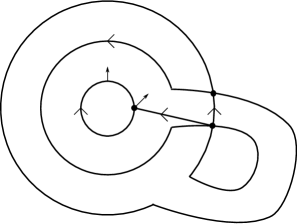
Generators for the cellular DGA are determined once we assign an indexing set to the sheets above each cell of . In all cases, if consists of sheets, we use for the indexing set in such a way that the -coordinates are non-increasing, . This uniquely specifies the indexing for cells that are not contained in the crossing locus. For such cells, it is convenient to specify the indexing of sheets by choosing a bordering -cell, and ordering sheets as they appear above this -cell. In Figure 11 the choice is indicated with arrows pointing from the cells in the crossing locus to a neighboring -cell.
In the definition of the cellular DGA, the generators associated to a given cell are placed into several, possibly distinct matrices depending on the context, eg. generators for a -cell may be placed into different matrices when computing the differentials of the two bordering -cells. When working through examples, it is convenient to fix particular matrices containing the generators of each cell and then write all differentials in terms of these initial matrices. For , we form initial matrices , and , as well as matrices , , , and by ordering rows and columns according to our indexing of sheets. All of these matrices are strictly upper triangular. We note that the matrices and have their -entry equal to and that there are no generators associated to cells that appear on the boundary of . We choose as for both and the initial point of
Differentials are then determined by the matrix formulas
| (23) | ||||
| (26) | ||||
Here, the notation (resp. ) indicates the matrix obtained from by inserting the block (resp. ) along the diagonal at row and column and In particular, In addition, is the permutation matrix associated to the transposition . Note that and are conjugated by in the formula for because the indexing of sheets above and was chosen to agree with the ordering above where sheets and appear in opposite order than they do above .
The cellular DGA of has generators. While the differential of each generator is easily obtained from the above matrix formulas, calculations with this version of the DGA would probably be handled best by a computer. However, applying Theorem 2.1 allows us to find a much smaller stable tame isomorphic quotient. We essentially cancel matrices of generators in pairs, following a sequence of simple homotopy equivalences applied to the polygonal decomposition of
Proposition 5.1.
The DGA of is stable tame isomorphic to a DGA, , with generators and of degrees
with differentials
Proof.
We will show how to cancel generators of the cellular DGA using Theorem 2.1 in order to arrive at as a stable tame isomorphic quotient. Throughout we use the same notation for generators and their equivalence classes in various quotients of , and we use the symbol to indicate that equality holds in the currently considered quotient.
Consider the equation
The -entries of and are both , so, using the notation , we have . The remaining entries of can be inductively canceled with the entries of , leaving
| (27) |
Proceeding in a similar manner, the equation
| (28) |
allows us to cancel all entries of , except for , with the corresponding entries of . In the quotient, we have
The equation for becomes
| (29) |
We can thus cancel as indicated in the following
The first and last equations imply and Finally,
| (30) |
We have canceled all generators except for and Since the result follows.
∎
Example 5.2.
Let denote copies of from Example 5.1 cusp-connect summed as in Figure 12. Each cell in Example 5.1 now has copies which we indicate with a superscript, such as Note that there is only one cell. We add a corresponding second superscript when labeling the Reeb chords; for example, the unique non-zero entry in is Except for the differentials are exactly as in (23) with appropriate subscripts. For example, For if we set equal to the start point of cell then
Proposition 5.2.
The DGA of is stable tame isomorphic to a DGA, , with generators of degrees
with differentials
As alluded to before, a partial computation for these examples appears in [15, Proposition 4.10 and Theorem 4.11]. In particular, using -holomorphic disks, the paper computes that the degree subspace of the linearized Legendrian contact homology is [Linearized LCH was introduced in [5]. Briefly, an augmentation, if it exists, is a DGA-morphism Define a graded algebra morphism on the generators by Define as the sum of words of length one in One can check that The linearized LCH is ] This computation agrees with ours. To see this consistency, note that since there are no generators of grading 0, there is a unique (graded) augmentation. Thus, the degree subspace of the linearized cellular homology is freely generated by and so isomorphic to
5.2. An example with swallowtail points
Consider the Legendrian, , which is pictured in Figure 6 together with a compatible decomposition of . As in the earlier example, we fix upper-triangular matrices by placing generators of into rows and columns according to the ordering of sheets above each cell. For the -cell that contains the crossing locus, we use the ordering of sheets as they appear above . (This choice of ordering is indicated in Figure 6 by the arrow pointing from to .)
The differential of any generator can be computed using the matrix formulas of Section 3.7. Here we write out and explicitly.
To compute we would consider the polygon pictured in Figure 6 that arises from considering the boundary of along with the location of the and decorations. Note that, for , the matrices and associated to the swallowtail points and are all equal to . Taking the upper vertex of for and , with the path around from to chosen to be counter-clockwise, we have
| (31) |
where is the permutation matrix of the transposition which appears because the labeling of sheets and above and is opposite. (Notations are as in Example 5.1.)
We now consider . As the ordering of rows and columns of agrees with the ordering of sheets above the and corners at the swallow tail points, we have
| (32) |
where
The cellular DGA for has generators, but once again appropriate applications of Theorem 2.1 produce a much smaller stable tame isomorphic quotient.
Proposition 5.3.
The cellular DGA of is stable tame isomorphic to a DGA with a single generator with and .
Remark 5.3.
This agrees with the DGA of the standard -dimensional Legendrian unknot, . In fact, it can be shown that and are Legendrian isotopic.
Proof.
We first compute
and apply Theorem 2.1 to cancel with so that and . (Again, denotes equality in the presently considered quotient.) Independent of the choices of and for the -cell , we have
so that we may cancel with .
Next, a parallel sequence of applications of Theorem 2.1 results in
For computing , we take and to be the vertex that is the common endpoint of and and choose the path around the boundary of to be clock-wise. We then have
In particular, we can use the following entry-by-entry evaluations to cancel all of the along with and as indicated:
where the terms and are in the subalgebra generated by entries of . (Hence, and satisfy the condition of the term from the statement of Theorem 2.1.)
5.3. Cone points
In this subsection, we extend the definition of the cellular DGA to allow for Legendrians whose front projections have cone point singularities.
The standard cone is the (non-generic) front projection of a Legendrian cylinder in . A point on the front projection of a Legendrian is called a cone point if there is a diffeomorphism of a neighborhood of in onto a neighborhood of that takes the front projection of to the standard cone. The inverse image in of a cone point singularity is an , so that neighborhoods of cone points in are topologically cylinders.
Consider a Legendrian with generic base and front projections except for the presence of finitely many cone points whose base projections are disjoint from the image of cusps and crossings. Write and for the base projection of cone points, and the remaining singular set of . Let be a polygonal decomposition of that contains (resp. ) in its -skeleton (resp. -skeleton).
We associate a DGA, , to as in Section 3 using with the following modification at a cone point. Assume that near a zero cell, , sheets of are labeled with the cone point connecting sheets and . Note that a Maslov potential on must have ; see the desingularization of the cone point in Figure 13.
-
(1)
The generators associated to are with and with
The corresponding upper triangular matrix, , (the -entry is ) satisfies . This same matrix is used when occurs as an initial or terminal vertex of a bordering -cell or -cell.
-
(2)
Choose a -cell that borders , and label one of the occurrences of as a vertex along with a . When computing for , we add an additional edge to at this vertex, and insert the matrix
(33) into the product of edges that appears in .
Proposition 5.4.
The DGA is equivalent to the cellular DGA of .
Proof.
By a small Legendrian isotopy, becomes front and base generic with the cone point replaced by swallowtail points, connected by -cusp edges, and -crossing arcs, cf. [7, Section 3.1]. In the base projection, the image of the cusp edges bounds a square, , whose vertices are swallowtail points. Two opposite corners of the square are upward swallowtails on the lower sheet of the cone point, and the other two opposite corners are downard swallowtails on the upper sheet. Crossing arcs appear as diagonals of the square. See Figure 13. There are sheets of above the interior of .
Produce from an -compatible polygonal decomposition (for this generic perturbation of ) by replacing the single -cell, , that was the cone point with the natural decomposition of the square into 4 triangles from Figure 13. Modify the -cells that had previously had endpoints at so that their endpoints are vertices of in such a way that the corner labeled with is replaced with some sequence of edges around the square starting with .
To prove the proposition we produce the cone point DGA from the cellular DGA via repeated application of Theorem 2.1. As a first step, we orient the boundary edges of consistently, and then cancel the generators associated to of the boundary edges of with the generators of their terminal vertex. The generators and differentials of these edges are simply
where all and matrices are with diagonal entries given by the appropriate or . (There are no or entries above the diagonal.) In the resulting quotient, generators of the three -cells have become , and generators associated to the vertices of are now equal. We use subscripts and for the matrices associated to the vertices of and the non-zero edge. See Figure 13.
[l] at 230 212 \pinlabel [l] at 230 74 \pinlabel [l] at 248 124 \pinlabel [bl] at 180 168 \pinlabel [b] at 124 248 \pinlabel [br] at 72 168 \pinlabel [t] at 124 -2 \pinlabel [tl] at 180 76 \pinlabel [r] at -2 124 \pinlabel [tr] at 72 76 \endlabellist
 \labellist\pinlabel [r] at -2 98
\pinlabel [r] at -2 144
\pinlabel [l] at 244 98
\pinlabel [l] at 244 144
\pinlabel [t] at 98 -2
\pinlabel [t] at 144 -2
\pinlabel [b] at 144 244
\pinlabel [b] at 98 244
\pinlabel [t] at 54 118
\pinlabel [l] at 124 52
\pinlabel [b] at 184 124
\pinlabel [r] at 118 182
\pinlabel at 70 66
\pinlabel at 178 66
\pinlabel at 178 176
\pinlabel at 70 176
\pinlabel [tl] at 126 116
\pinlabel [tr] at 32 44
\endlabellist
\labellist\pinlabel [r] at -2 98
\pinlabel [r] at -2 144
\pinlabel [l] at 244 98
\pinlabel [l] at 244 144
\pinlabel [t] at 98 -2
\pinlabel [t] at 144 -2
\pinlabel [b] at 144 244
\pinlabel [b] at 98 244
\pinlabel [t] at 54 118
\pinlabel [l] at 124 52
\pinlabel [b] at 184 124
\pinlabel [r] at 118 182
\pinlabel at 70 66
\pinlabel at 178 66
\pinlabel at 178 176
\pinlabel at 70 176
\pinlabel [tl] at 126 116
\pinlabel [tr] at 32 44
\endlabellist
Notations for cells in the interior of are indicated in Figure 13. Above the -cells and -cells in the interior of , we label sheets from to as they appear above the neighboring -cell indicated by the small arrows in Figure 13. This ordering specifies the notation for generators. In this proof, the notation for matrices is fixed, so that, eg., the matrix always has rows and columns ordered according to the ordering of sheets above , and is always ordered as above . The crossing locus results in the following entries above the diagonal:
Matrix entries and
As in Section 3.13, for computing differentials of -cells containing swallowpoints, we add additional edges at corners labeled with or . We notate the matrices associated to these edges as illustrated in Figure 13. These matrices are
For the -cells (resp. , ), we choose initial and terminal vertices to be the endpoints of (resp. of ). We have differentials
where the matrices and are permutation matrices for the transpositions and , and .
We begin to cancel generators. First, observe that
and use Theorem 2.1 to cancel the boxed generators. [The product of strictly upper triangular matrices has all -entries , so the -entry of is the sum of the -entries from , , , and .] The remaining non-zero entries of are in correspondence with those of , so we cancel
[The condition on the ordering of generators required to apply Theorem 2.1 is verified as in proof of Theorem 4.3.] Note that in the quotient, we have
so we can compute and cancel
Record that
With non-zero entries of and now in correspondence, cancel
This gives , so that
Hence, we can modify our usual orderings of generators (arising as in Lemma 4.1) by moving to be the first generator. This allows us to cancel all entries of other than (the entry of is ) by
With already canceled, the remaining generators in are in correspondence with those from ; cancel
To summarize where we are, the only remaining generators associated to the cells of are and the entries of , , and except for which has . We have
Using gives
Then, gives
[The range of in the summations is different from in the definitions of and because .] Next, compute
where
and
Using that and shows that
so we compute
Combining the previous computations gives
Observe that is upper triangular with -entry .
Next, since the -entries of , , and are all , the formula for shows
After making this cancellation,
and another careful matrix multiplication shows
This matrix has all above diagonal entries in the and rows and columns equal to . Thus, the entries of in these rows and columns agree with the entries of , and we have, for and ,
Here, we cancel beginning with (resp. ), and then with decreasing (resp. increasing), so that inductively when we cancel the equation simplifies to
Thus, all of the , , , , and are in the quotient. The remaining generators from are in correspondence with the generators, and we cancel
In the quotient, we have and
which gives the relations
At this point all generators above the square have been canceled except for with . Moreover, the matrix associated to each of the corners of is , and to all of the outer edges is except for the edge labeled in Figure 13 which has with as in the definition of the DGA with cone points. Thus, the appearances of in the differential of bordering cells matches the definition of the cone point DGA. ∎
5.4. 1-cells with more than one crossing or cusp arc
Often it is possible to relax the requirement that at most crossing or cusp arc lies above each -cell. We do not attempt to give the most general statement here, but restrict ourselves to an illustrative example that will be useful for the class of examples in Section 5.6.
For , suppose that is a polygonal decomposition of that is -compatible except near a -sided simple closed curve contained in the -skeleton of . In a neighborhood of , there appear several crossing arcs that project to small shifts of in the normal direction, and no other crossing or cusp arcs. See Figure 14. Above , is a union of sheets that project homeomorphically to . Suppose further that no two sheets of cross each other more than once above .
[tr] at 46 58 \endlabellist

With this set-up, we associate a variant of the cellular DGA to . For definiteness of notation, choose one side of , and label the sheets of as in the order they appear above this side of . Let be the permutation such that appears in position on the other side of . Note that for , and cross above if and only if . To each -cell (resp. -cell) of , assign generators (resp. ) for all with . (So multiple pairs of crossing sheets contribute to multiple 0s to the upper triangle, as in the single crossing case.) The differential is defined as in the case of the cellular DGA: -cells in have ; -cells in have ; when a -cell or -cell appear in the boundary of a -cell, we place the generators into matrices or being sure to order rows and columns using the ordering of sheets above the -cell. For instance, above -cells on the side of where sheets of above appear in order (resp. ) generators associated to a bordering -cell in are placed as (resp. where is the permutation matrix .)
Proposition 5.5.
The DGA is stable tame isomorphic to the cellular DGA of .
Proof.
For simplicity, we consider the case when the decomposition of consists of a single -cell at and -cell at in detail, with a similar argument applying in general. We produce a -compatible polygonal decomposition from by replacing the decomposition of the single closed curve, , with a decomposition as in Figure 15; using coordinates , we take the crossing arcs in to be at , each decomposed into a -cell, and a -cell . Additional -cells are given by running perpendicularly through the annulus connecting the -cells of the different crossing arcs. See Figure 15
Denote the Cellular DGA of by . We place generators of corresponding to the translates of the original - and -cell of into matrices , , for , and place the generators corresponding to vertical product cells of the form (resp. into matrices , , for . For the and we take the ordering of sheets (and labeling of generators) to agree with the ordering in the bordering region that has smaller -coordinate. In this proof, these notations for matrices are fixed (including the ordering of rows and columns).
[r] at 472 4 \pinlabel [r] at 472 36 \pinlabel [r] at 472 68 \pinlabel [r] at 472 100 \pinlabel [l] at 482 20 \pinlabel [l] at 482 52 \pinlabel [l] at 482 84 \pinlabel [l] at 536 20 \pinlabel [l] at 536 52 \pinlabel [l] at 536 84 \pinlabel [t] at 598 4 \pinlabel [t] at 598 36 \pinlabel [t] at 598 68 \pinlabel [t] at 598 102

To describe the differential, let be the sequence of transpositions corresponding to the crossing arcs as increases from to . So, if the crossings occur at , then the sheet in position immediately before is in position after . Notice that the products
then have the property that the sheet labeled before is labeled after . In particular, the permutation defined prior to the statement of the proposition is .
For the subalgebra generated by the and generators (above ) we have
[The -entry of is .] We cancel all of the and generators with and some of the generators via the following inductive procedure.
To begin, for , cancel with , and for , cancel [We apply Theorem 2.1 repeatedly, so that increases as we go. Thus, any terms that appear in are already when the theorem is applied.]
For , inductively suppose that we have canceled all of the generators of with , and with , as well as all entries with the property that the sheets labeled and before cross one another at some . Moreover, suppose that in the quotient, we have
and when and cross before .
Then, the differential becomes
Note that the final term is ; it is upper-triangular (because of the entries that are equal to .) For , we cancel and . For , we cancel
[This entry has not yet been canceled because of the assumption that no two sheets cross each other more than once in .] In the quotient, since , it follows that
and so that the induction proceeds.
At the conclusion of the procedure, the only remaining generators are those entries of corresponding to sheets that do not cross one another above , and we have
| (34) |
At this point, differentials of the have simplified as
Then, using a similar inductive procedure, we can cancel all of the and for , as well as those entries of corresponding to sheets and that cross somewhere in . In the quotient, we have the relation
| (35) |
The remaining generators in this final quotient of are exactly as in the description of , and the differentials agree as well in view of the relations (34) and (35).
∎
5.4.1. Extension to multiple cone points
The DGA with cone points from Proposition 5.4 has a similar easy extension to the case where has several cone points projecting to the same point . Suppose that above there are cone points joining the pairs of sheets . In this case, form a DGA as in Proposition 5.4 with the two modifications:
-
(1)
The -cell at has generators with and for all .
-
(2)
The matrix where
(36)
Proposition 5.6.
The resulting DGA is equivalent to the DGA from Proposition 5.4.
Proof.
To see this, isotope the front projection of so that the cone points appear at distinct points of in a small neighborhood of . Then, form a cellular decomposition where the single -cell at is expanded to a string of -cells, at cone points connected by a sequence of -cells, , all located in the corner of that was labeled with . All of the generators for the , and , as well as the -entries of are canceled by a sequence of applications of Theorem 2.1. (At the inductive step, cancel with all of the generators of and the entries of for .) When computing the differential of -cell that contains the string of -cells and -cells, the contribution to the product of edges from this corner is the product of the individual matrices
and in the quotient for all . ∎
5.5. Front spinning a Legendrian knot
In this subsection, we show how the DGA of a surface which is the front-spin of a 1-dimensional Legendrian knot can be derived from the DGA of the knot. The result agrees with known computations when the axis of rotation and the knot do not intersect, and provides new examples when the axis and knot do intersect.
5.5.1. The suspension of a DGA
We begin with some algebraic preliminaries, which are motivated by a homotopy theory for DGAs (or more generally for differential graded operad algebras where the operad might not be the associative one). Suppose is a DGA freely generated by triangular with respect to these generators (see Section 2.1.1), possibly unital, and with an arbitrary coefficient ring. Define the suspension of as follows:
-
•
is freely generated by
-
•
the grading of is the same as it is in while
-
•
and where is a derivation defined by its image of the generators (So for example, if is unital, and )
We assume is unital if is.
We also consider a variation of this construction. Let be a sub-DGA of generated by some subset of the generating set. Define the suspension of relative to to be the DGA as above except that for all elements
Lemma 5.1.
If and are stable tame isomorphic then so too are and If is a sub-DGA as above of both and and the elementary automorphisms in the definition of stable-tame isomorphism fixes then the suspensions of and relative to are stable tame isomorphic.
Proof.
It is easy to check that if is a stabilization with new generators then with new generators So assume is an elementary isomorphism, defined on generators as (In the language of Section 2.1.1, while is the identity on all other generators.) We claim the algebra isomorphism defined on generators by
is a (tame) DGA isomorphism.
First note that This is obvious on generators, while the inductive (on word-length) step follows from linearity and the following relation on monomials:
First note that since then for generator For the other generators,
These are equal by the relation above.
If the suspensions are relative, the same formulas and arguments apply after recalling that for ∎
5.5.2. Spun cellular decomposition
Let denote the standard contact structure. Let be the lower-dimensional analog of the front projection Let be a Legendrian embedding of the union of (a non-negative ) number of circles sitting in as well as a (non-negative) number of arcs in whose endpoints sit on the -axis. We impose the following condition on the front projections of the arcs in If we reflect the arcs’ fronts through the -axis, the arcs and their reflections must glue together to form the front of a collection of (smooth) Legendrian circles. An arbitrary Legendrian embedding of circles and arcs can achieve these conditions with a Legendrian isotopy. Embed as Consider the rotation about the -axis, as defined in [15, Section 4]. We say that the front spin of is the Legendrian surface in standard contact whose front is given by this rotation. Note that is a Legendrian embedding of a collection of spheres and/or tori. In the case when two arc endpoints have the same front projection in then the spun surface has a cone point. We consider Legendrians with possibly multiple pairs of matching arc-front-endpoint conditions, but we assume no three arcs have fronts with the same endpoint.
Consider a cellular decomposition of where in the case that has a Legendrian arc, the decomposition includes as a 0-cell. For each cell of excluding the 0-cell if it appears, we associate two cells for which we denote by and The first is simply the cell after embedding as The second is the embedded spun about the -axis; that is, a radially symmetric map of with the ends and mapping to the same cell as . Note that the crossing/cusp 0-cells become analogous 1-cells under spinning.
If is a 0-cell of then we denote by again the 0-cell of As mentioned above, if represents a crossing 0-cell of then the corresponding cell in sits below a cone point.
5.5.3. The cellular DGA of a front spin
Proposition 5.1.
Proof.
This can be deduced from a (greatly shortened) argument along the lines of the isomorphism between the Cellular DGA and LCH proved for -dimensional Legendrians in [35].
However, this is not necessary, since in the -dimensional case the Cellular DGA is almost identical to the LCH DGA as computed after the addition of splashes or dips, [23], [37]. To give a definite isomorphism, we use the version of splashes from [24] where the generators and differentials for the LCH DGA of a -dim Legendrian are stated in Propsition 4.1 of [24]. There is broken into a product of elementary tangles containing either a single left cusp, right cusp, or crossing. To the right of the -th elementary tangle, a collection of splashes is given (for all ), and this produces two upper triangular matrices of generators labeled in [24] as and . In addition, when there is a crossing (resp. right cusp) in the -th elementary tangle, there is a single generator (resp. ).
A -compatible polygonal decomposition of arises in an obvious way by taking the -cells to occur at cusps and crossings. Label the - and -cells, so that from left to right they appear as . If we identify the Cellular DGA generators and with and respectively, then the differentials almost agree. The differences are the following:
-
(1)
At -cells with crossings, there are more generators, and , in the LCH DGA.
-
(2)
At -cells with right cusps, there are more generators, , , , , , and .
Repeated applications of Theorem 2.1 (that the reader may by now find routine) cancel these generators in pairs. In this quotient of the LCH DGA, the differential agrees precisely with the Cellular DGA differential.
∎
We can now state the main proposition of Subsection 5.5
Proposition 5.2.
-
(1)
Suppose has no arc components. The DGA is the suspension of
-
(2)
Suppose has arc components whose front projections have distinct endpoints. The DGA is the suspension of relative to the sub-DGA associated to the 0-cell.
-
(3)
Suppose has arc components whose front projections have pairs of matching endpoints. The DGA is the suspension of relative to the sub-DGA associated to the 0-cell, with the following modification. Let be the matrix of generators above the 0-cell. We replace with from equation (36).
Proof.
As we see from Sections 3.6.1 and 3.6.2 that for each generator of type and in the cellular has a pair of generators generators and A quick check shows for either type of generator. (If sits above the 0-cell there are no new generators of type )
Let denote the suspension of which a priori may not equal We first verify that This holds by definition in case (1) and by a tautology in case (2), so consider case (3). Recall is the matrix of elements sitting over the 0-cell
Recall Assume we have shown that if Then the general case follows from induction:
Since and from (33) it suffices to show
Recall Let denote the -entry of the matrix and denote the Kronecker delta. We compute each entry of each term in each of the four left hand side summands.
So the second and third summands cancel, while the first and fourth match the first and second on the right hand side.
Let and denote the strictly upper-triangular matrices of generators as in Section 3.6, modified appropriately if a crossing or cusp pair is involved. Then is given by (2), are given by (3), and is given by (4). We verify the identity for as is easier and are immediate.
Let denote the -cells used to define the cellular DGA of We use polar coordinates for to refer to the -cells (polar lines) and -cells (polar rectangles) which define the cellular DGA of For example, all 1-cells that contain cusp or crossing loci are on lines. If a -cell is indicated to lie on (resp. ), this means that we consider the -cell as the boundary of a -cell lying counter-clockwise (resp. clockwise) to it. We orient all -cells in the positive polar coordinate direction. Fix a -cell with initial and terminal vertices We use below that and Also, for the relative suspension case (so ), equals the 0 matrix when there are no cone points in case (2), and equals when there are in case (3).
∎
5.5.4. A comparison with older front-spun computations
The first case (where there are no Legendrian arcs) is already known in the literature. The second two cases (Legendrian arcs spinning to possibly induce cone points, or not) are new.
Corollary 5.1.
The cellular DGA computation in the first example agrees with pre-existing computations of the LCH DGA, up to stable tame isomorphism.
Proof.
A partial computation of the LCH DGA of this example was done, up to certain quadratic terms, in [15, Proposition 4.17]. The complete LCH computation was done in [19, Theorem 1.1], which states that up to stable tame isomorphism, the LCH DGA of is the suspension of the LCH DGA of The result then follows from Lemma 5.1 and Propositions 5.1 and 5.2. ∎
5.6. A family of examples
The following generalizes a family of Legendrian spheres considered in [3].
We introduce Legendrians, , where ,
-
•
is a permutation with the property that
-
•
and satisfies .
To construct , start with copies of the standard -dimensional Legendrian placed vertically above one another so that their left and right cusps all share common -coordinates. For some pairs of unknots, the lower strand of the upper unknot crosses the upper strand of the lower unknot twice to form a Hopf link. This is specified by the permutation as follows: Labeling the strands near left cusps in with descending -coordinate as , for the -th strand crosses the -th strand twice if and only if . Arrange that the front diagram is symmetric, so that when we spin the front diagram around the midpoint (in the -direction) it produces a stack of two dimensional unknots with one circular crossing arc for each with . Call this spun front .
Next, to the right of the previously constructed front, we create one more Legendrian sphere, . Begin with a single -dimensional unknot; apply consecutive Type 1 Reidemeister moves to produce a front with left cusps and crossings. Then, spin around the midpoint to produce a -dimensional Legendrian sphere that is standard -dimensional unknots joined together by a sequence of cone points.
Finally, to arrive at , we connect these two pieces by joining the -th unknot from to the -th cusp edge from by a tube whose cross-sections are Legendrian unknots. Here, we label the unknots of with descending -coordinate, but label the cusp edges of with ascending -coordinate, starting with . See Figure 16.
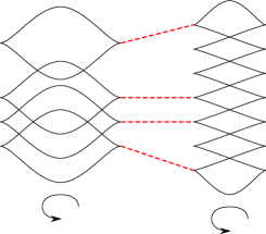
Theorem 5.4.
The DGA of is equivalent to a DGA with generators
and differentials
The grading is given by
where and .
The crossing configurations that lead to terms in are depicted in Figure 17. We prove Theorem 5.4 at the end of this subsection.
[r] at -5 344 \pinlabel [l] at 64 320 \pinlabel [l] at 64 368 \pinlabel [l] at 90 344 \pinlabel [r] at 470 344 \pinlabel [l] at 586 320 \pinlabel [l] at 586 352 \pinlabel [l] at 586 392 \pinlabel [l] at 586 280 \pinlabel [l] at 614 344 \pinlabel [r] at 4 94 \pinlabel [l] at 130 152 \pinlabel [l] at 130 82 \pinlabel [l] at 130 42 \pinlabel [l] at 130 114 \pinlabel [l] at 194 94 \pinlabel [l] at 482 40 \pinlabel [l] at 482 0 \pinlabel [l] at 482 82 \pinlabel [l] at 482 152 \pinlabel [l] at 532 94

Among the , there are many examples of pairs of Legendrians whose linearized homology groups have identical ranks, but are distinguished by the ring structure on linearized cohomology. We briefly recall the definition of the ring structure. Let be a graded augmentation, and write where denotes the linear -span of the generators of . The conjugated differential
has the form
Dualizing gives operations
The linearized cohomology complex is , and the operation descends to a well defined associative product of degree on the linearized cohomology
The set of isomorphism types of the rings
depends only on the stable tame isomorphism type of and is hence a Legendrian isotopy invariant [6].
Observe that for any there is at least one augmentation, , such that . (Take to vanish identically on generators.) Moreover, for , the operation is independent of (due to the absence of monomials of degree or more in ). Thus, the ring structure on is independent of the choice of (with ). This ring is an invariant of .
For example, consider the case where is
the Poincare polynomial of is
By choosing the sequence appropriately, this can be an arbitrary polynomial of the form
| (37) |
for any .
Proposition 5.7.
-
(1)
For arbitrary , there exists and such that the groups
have the same Poincare polynomial.
-
(2)
If there exists with such that , then these groups are not isomorphic as rings. In particular, and are not Legendrian isotopic.
Recall that for all -dimensional Legendrian spheres in standard contact such as the “classical” Legendrian invariants do not contain any information: there is only one smooth isotopy class, the Thurston-Bennequin number is 1, and the rotation class vanishes [15].
Proof.
(1) follows since for arbitrary the Poincare polynomial has the form given in (37).
(2) follows since in , the image of is -dimensional. (It is the span of .) However, when has and , there is some such that . This implies that , so that the image of has dimension or more. ∎
As a specific example where (2) applies, consider
Remark 5.5.
Proof of Theorem 5.4.
We use the extended version of the cellular DGA from Propositions 5.5 and 5.6, so we work with a decomposition of where all of the crossing arcs (resp. cone points) of (resp. ) correspond to a single circle (resp. single -cell) in the -skeleton of . Moreover, by methods similar to those used in the proof of Proposition 5.5, we can position the cusp arcs so that together their projection is as in Figure 18. In more detail, the cusp edges of the part of all project to a circle in ; the cusp edges that are part of to the left of (i.e., together with the tubes connecting to ) project to an arc with two end points on the circle. This leads to the cellular decomposition pictured in Figure 18. Since the cusp edges above any given edge all involve distinct pairs of sheets, the only modification to the usual definition of the DGA is that when computing the differential of bordering cells, at -cells (resp. -cells) we insert one block (resp. block) for every pair of sheets that cusp above the -cell. In particular, above the -cells and the associated matrices have blocks all along the diagonal.
at 80 82 \pinlabel at 186 106 \pinlabel at 330 116 \pinlabel [bl] at 180 62 \pinlabel [r] at 116 82 \pinlabel [tr] at 240 36 \pinlabel [b] at 232 128 \pinlabel [tr] at 60 45 \pinlabel [l] at 310 82 \pinlabel [l] at 228 92 \pinlabel [l] at 280 62

Step 1. Canceling generators in the part of .
Above , has sheets. We have differentials
| (38) | ||||
| (39) |
where
| (40) |
That is, is block diagonal with the blocks along the diagonal.
Note that the matrix has ’s in the entries. Therefore, we compute from (38)
Thus, we can adjust our usual triangular partial ordering of generators (as in Lemma 4.1), , by taking these to be the smallest generators. With this adjustment to the ordering, for all with , we can cancel
where (canceling with increasing), the term belongs to the sub-algebra generated by generators that are strictly smaller than with respect to . In the quotient, we have
and the latter equality shows that
| (41) |
Thus, for we can cancel
We DO NOT cancel . Instead, set , and observe that
| (42) |
Finally, we cancel all remaining generators, with themselves; note that (39) gives for ,
where belongs to the sub-algebra generated by generators satisfying , and similar for .
To summarize, the only generator remaining from the matrices is whose differential is given by (42)
Step 2. Canceling generators in the part of .
Above , has sheets. The matrices have generators in all of there entries with . The matrices and have generators and in the entries with and , with the remaining entries (as specified Proposition 5.5). There are no generators associated to the vertices and As indicated in Figure 18, we label sheets above these cells as they appear above . The notation for these matrices is fixed. We have differentials
| (43) | ||||
| (44) | ||||
| (45) |
Recall so that the -entry of is
Start by canceling
Observe, that in the quotient
| (46) |
(because the -entry of and is since both factors are upper triangular, and the -entry of is the sum of the -entries of the three factors).
Next, we will cancel as many of the entries of with as we can. When doing so, in order to meet the hypothesis of Theorem 2.1, we will need to modify the ordering of generators. For the entries of and , we require that if and only if (where each of and has the form or ). Remaining generators are all larger than those from and and are ordered as in Lemma 4.1.
With this ordering, we can cancel
In the quotient, the values of are as follows, depending on the parity of and :
| (47) |
[These formula are verified using induction on and the relation
In doing so, it is useful to note that if is not in the quotient then, since , we must have even and odd.]
The generators with and will not be canceled. They have differentials
| (48) |
[At the first equality, note that there is no generator, and for the second equality use that unless is even.]
Finally, we cancel as many entries of as we can with the entries of , using
In doing so, it is convenient to rewrite (44) as
giving the entry-by-entry formula
Thus, for all with , we cancel
[To apply Theorem 2.1, we order so that all entries of are greater than all entries of (the generators belong to the subalgebra generated by the generators in the current quotient), and so that if and only if .] All generators with and remain in the quotient. For such generators, is even and is odd so we use (47) to compute
| (49) | ||||
Note that these formulas agree with those from the statement of the theorem with the role of and interchanged.
To summarize, in Step 1 and Step 2 we have now cancelled all of the generators besides and those and with and . The differentials of the and have been computed in (48) and (49). It remains only to calculate . Using that
[At the second equality, we used that the condition on the first (resp. second) summation implies crosses (resp. crosses ), so is odd (resp. even).] Since
the result follows. [The second equality uses that is unless there is a tube connecting one of the unknots on the left to the -th cusp edge. The final inequality uses (46).]
∎
References
- [1] V.I. Arnold, S. M. Gusein-Zade, A.N. Varchenko. Singularities of differentiable maps. Volume 1. Modern Birkhauser Classics, Monogr. Math., 82, Birkh user Boston, Boston, MA, 1985
- [2] Frederic Bourgeois, Tobias Ekholm and Yakov Eliashberg. Effect of Legendrian surgery. Geom. Topol. 16 (2012), no. 1, 301–389
- [3] F. Bourgeois, J. Sabloff, L. Traynor. Lagrangian cobordisms via generating families: construction and geography. Algebr. Geom. Topol. 15 (2015), no. 4, 2439–2477
- [4] B. Chantraine Lagrangian concordance is not a symmetric relation Quantum Topology 6 (2015), No. 3, 451-474.
- [5] Yuri Chekanov. Differential algebra of Legendrian links. Invent. Math., 150 (2002), no. 3, 441–483.
- [6] Gokhan Civan, John B. Etnyre, Paul Koprowski, Joshua M. Sabloff, Alden Walker. Product structures for Legendrian contact homology. Mathematical Proceedings of the Cambridge Philosophical Society (2011) 150:02, 291–311.
- [7] Georgios Dimitroglou Rizell. Knotted Legendrian surfaces with few Reeb chords, Alg. Geom. Top. 11 (2011) 2903–2936.
- [8] Georgios Dimitroglou Rizell. Legendrian Ambient Surgery and Legendrian Contact Homology , ariv: 1205.5544
- [9] Georgios Dimitroglou Rizell and Roman Golovko. Estimating the number of Reeb chords using a linear representation of the characteristic algebra ariv:1409.6278
- [10] Tobias Ekholm. Morse flow trees and Legendrian contact homology in 1-jet spaces. Geom. Topol., 11:1083–1224, 2007.
- [11] T. Ekholm, Y. Eliashberg, E. Murphy, and I. Smith. Constructing exact Lagrangian immersions with few double points GAFA, 23 (2013), no. 6, 1772–1803.
- [12] T. Ekholm, J. Etnyre, and J. Sabloff. A duality exact sequence for Legendrian contact homology. Duke Mathematical Journal. 150 (2009), no. 1, 1–75
- [13] Tobias Ekholm, John Etnyre, Lenny Ng, and Michael Sullivan. Knot contact homology. Geom. Topol. 17 (2013), no. 2, 975–1112
- [14] Tobias Ekholm, John Etnyre, and Michael Sullivan. The contact homology of Legendrian submanifolds in . J. Differential Geom., 71(2):177–305, 2005.
- [15] Tobias Ekholm, John Etnyre, and Michael Sullivan. Non-isotopic Legendrian submanifolds in . J. Differential Geom., 71(1):85–128, 2005.
- [16] Tobias Ekholm, John Etnyre, and Michael Sullivan. Orientations in Legendrian contact homology and exact Lagrangian immersions. Internat. J. Math. 16 (2005), no. 5, 453–532.
- [17] Tobias Ekholm, John Etnyre, and Michael Sullivan. Legendrian contact homology in . Trans. Amer. Math. Soc., 359(7):3301–3335 (electronic), 2007.
- [18] Tobias Ekholm, Tamas Kalman and Ko Honda. Legendrian knots and exact Lagrangian cobordisms. ariv:1212.1519.
- [19] Tobias Ekholm and Tamas Kalman. Isotopies of Legendrian 1-knots and Legendrian tori. J. Symp. Geom., 2008, no 4, 407–460.
- [20] Tobias Ekholm, Lenny Ng, and Vivek Shende. A complete knot invariant from contact homology. ariv:1606.07050
- [21] Yakov Eliashberg. Invariants in contact topology, Proceedings of the International Congress of Mathematicians, Vol. II (Berlin, 1998). Doc. Math. 1998, Extra Vol. II, 327–338.
- [22] Yakov Eliashberg, Alexander Givental, and Helmut Hofer. Introduction to symplectic field theory, Geom. Funct. Anal., 2000, Special Volume, Part II, 560–673.
- [23] D. Fuchs, The Chekanov-Eliashberg invariant of Legendrian knots: Existence of augmentations. J. Geom. Phys. 47 (2003), no. 1, 43-65.
- [24] D. Fuchs, D. Rutherford. Generating families and Legendrian contact homology in the standard contact space. J. Topol. 4 (2011) 190 226.
- [25] Cameron Gordon and Tye Lidman. Knot contact homology detects cabled, composite, and torus knots. ariv:1509.01642
- [26] John Harper and Michael Sullivan. A bordered Legendrian contact algebra J. Symp. Geom., 2014, no 2, 237-255.
- [27] Allen Hatcher and John Wagoner. Pseudo-isotopies of compact manifolds. Asterisque, No. 6. Soc. Math. de France, Paris, 1973. 275 pp.
- [28] Michael B. Henry and Daniel Rutherford. A combinatorial DGA for Legendrian knots from generating families. Commun. Contemp. Math. 15 (2013), no. 2, 1250059, 60 pp.
- [29] Michael B. Henry and Daniel Rutherford. Ruling polynomials and augmentations over finite fields. J. Topology 8 (2015), no. 1, 1-37
- [30] Mark Lowell. A Seifert-van Kampen Theorem for Legendrian Submanifolds and Exact Lagrangian Cobordisms. ariv:1511.03375.
- [31] Lenny Ng. Computable Legendrian invariants. Topology 42 (2003), no. 1, 55–82.
- [32] Lenny Ng. Framed knot contact homology. Duke Math. J. 141 (2008), no. 2, 365–406
- [33] Lenhard Ng, Dan Rutherford, Vivek Shende, Steven Sivek and Eric Zaslow Augmentations are Sheaves. ariv:1502.04939
- [34] D. Rutherford, The Thurston-Bennequin number, Kauffman polynomial, and ruling invariants of a Legendrian link: The Fuchs conjecture and beyond, Int. Math. Res. Not. (2006), Art. ID 78591.
- [35] Dan Rutherford and Michael Sullivan. Cellular computation of Legendrian contact homology for surfaces, Part II. Preprint.
- [36] Dan Rutherford and Michael Sullivan. In preparation.
- [37] J. M. Sabloff, Augmentations and rulings of Legendrian knots, Int. Math. Res. Not. 2005, no. 19, 1157–1180.
- [38] Steven Sivek. A bordered Chekanov-Eliashberg algebra J. Topology 4 (2011), no. 1, 73–104.