Tricriticality in Crossed Ising Chains

Abstract

We explore the phase diagram of Ising spins on one-dimensional chains which criss-cross in two perpendicular directions and which are connected by interchain couplings. This system is of interest as a simpler, classical analog of a quantum Hamiltonian which has been proposed as a model of magnetic behavior in Nb₁₂O₂₉ and also, conceptually, as a geometry which is intermediate between one and two dimensions. Using mean field theory as well as Metropolis Monte Carlo and Wang-Landau simulations, we locate quantitatively the boundaries of four ordered phases. Each becomes an effective Ising model with unique effective couplings at large interchain coupling. Away from this limit we demonstrate non-trivial critical behavior, including tricritical points which separate first and second order phase transitions. Finally, we present evidence that this model belongs to the 2D Ising universality class.

I Introduction

Dimensionality, along with order parameter symmetry, plays a decisive role in the occurrence of phase transitions and the critical exponents with which they are characterizedlavis15 . Beginning with simple, regular geometries, critical properties are now well-understood in more complex geometries in which the dimensionality is more ambiguous, including diluted latticesyeomans79 , fractal geometriesgefen80 , and networks with longer range interactionsbaker63 ; nagle70 ; scalettar91 ; gitterman00 ; lopes04 .

Recently there has been interest in a further class of systems of “mixed geometry” whose underlying structure consists of two perpendicular collections of one dimensional chains which are then further connected to form a two dimensional framework. For example, it has been suggestedlee15 that an appropriate model of magnetic phase transitions in one of the niobates, Nb₁₂O₂₉, consists of one dimensional chains of localized (Heisenberg) spins and a further perpendicularly oriented set of one dimensional conduction electron chains. These two types of spins reflect the presence of distinct Nb cations with 4d¹ configuration, one of which exhibits local moment behavior and the other being itinerant and Pauli paramagneticcava91 ; andersen05 . In this model, the electron spins on the conducting nanowires are coupled to the Heisenberg chains by a Kondo interaction on each site.

Similarly, in optical latticesgreiner08 , bosonic or fermionic atoms can occupy higher, spatially anisotropic, $p_{x}$ and $p_{y}$ orbitals which allow hopping which is essentially just along one-dimensional chains. Within a given well, atoms can convert from occupying the $p_{x}$ to occupying the $p_{y}$ orbital, thus coupling the perpendiular chains and providing a two dimensional character to the system. Bosonic systems in this geometry can exhibit exotic forms of superfluidity whose condensate wave functions belong to non-trivial representations of the lattice point group, with condensation accompanied by unusual columnar, antiferromagnetic, and Mott phases isacsson05 ; liu06 ; wu09 ; hebert13 . Models in which fermionic degrees of freedom in the two orbitals have Hund’s rule type coupling have also been considered, and shown rigorously to exhibit magnetic orderli14 .

These examples share a common “${\rm 1D}\times{\rm 1D}$” geometrical structure in which one type of chain has degrees of freedom which are coupled in the $\hat{x}$ direction, while the degrees of freedom of the other couple in the $\hat{y}$ direction. An additional interaction on each lattice site connects the two sets of chains. Although considerable progress has been made in modeling the niobates and p-wave bosons in optical lattices, in both cases the quantum nature of the spins makes achieving a definitive understanding of the critical phenomena quite challenging. The goal of this paper is to examine a classical Ising model on this type of lattice. We will show that the interchain coupling is sufficient to promote long range order at finite temperature, and that the phase transitions can exhibit a rich variety of behaviors including tricritical points.

II Model and Methods

We consider the following model,

$$E= -J_{x}\sum_{\bf r}S_{\bf r}S_{{\bf r}+\hat{x}}-J_{y}\sum_{\bf r}T_{\bf r}T_{{\bf r}+\hat{y}}$$

$$-J_{z}\sum_{\bf r}S_{\bf r}T_{{\bf r}}-J_{z^{\prime}}\sum_{\bf r}S_{\bf r}\,(\,T_{{\bf r}+\hat{y}}+T_{{\bf r}-\hat{y}}\,)$$

$$-J_{z^{\prime}}\sum_{\bf r}T_{\bf r}\,(\,S_{{\bf r}+\hat{x}}+S_{{\bf r}-\hat{x}}\,)$$ (1)

which we will refer to as the crossed Ising chains model (CICM).

Here $S_{\bf r}$ and $T_{\bf r}$ are Ising spins (i.e. they can have a value of either +1 or $-1$) coupled into one-dimensional chains in the $\hat{x}$ and $\hat{y}$ directions, respectively. These spins occupy a two-dimensional, square, $L$ $\times$ $L$ lattice with periodic boundary conditions. There is an S and a T spin on each of the $N$=$L^{2}$ sites and therefore, 2$N$ total spins in the system. $J_{z}$ and $J_{z^{\prime}}$ couple S and T spins on the same lattice site and near neighbor sites, respectively. The geometry of Eq. (1) is illustrated in Fig. 1. For simplicity, and also because this choice is the appropriate one for several of the physical realizations of the CICM, we will set $J_{x}=J_{y}=J_{x,y}=1$ and measure all energies in units of $J_{x,y}$.

Initial insight into the phase diagram of this model is obtained by considering $T=0$ and minimizing the internal energy, Eq. (1). Fig. 2 shows the definitions of the four ordered phases which can occur: ferromagnetic (FM), ferromagnetic-prime (FM^′), antiferromagnetic (AFM), and antiferrmagnetic-prime (AFM^′). The phase diagram at $T=0$ is shown in Fig. 3. The CICM has the symmetry that changing $J_{z}\to-J_{z}$ and $J_{z^{\prime}}\to-J_{z^{\prime}}$ changes the phase from FM $\to$ AFM or AFM $\to$ FM, and FM^′ $\to$ AFM^′ or AFM^′ $\to$ FM^′. If $J_{z}$ and $J_{z^{\prime}}$ are both positive or both negative, there will be no competition between ordered phases and the model will have relatively uninteresting features, namely a conventional second order phase transition between a high temperature disordered paramagnetic (PM) phase and a low temperature FM phase or AFM phase, respectively. However, if only one of the interchain couplings is negative, there will be a competition between ordered phases and the most interesting physics will result.

The total spin, $S_{\bf r}+T_{\bf r}$, on a site can take on the three values, $-2,0,\text{or}+2$, giving the CICM some similarity to the two-dimensional square lattice Blume-Capel model blume66 ; capel66 ,

$$E=-J\sum_{\langle ij\rangle}M_{i}M_{j}+\Delta\sum_{i}M_{i}^{2}$$ (2)

which is a spin 1 generalization of the Ising model where $M_{i}=-1,0,\text{or}+1$. The choice $J_{z}<0$ favors $S_{\bf r}=-T_{\bf r}$ and hence $S_{\bf r}+T_{\bf r}=0$ so that the strength of $J_{z}$ plays a role similar to that of the vacancy potential $\Delta$ whose energy $\Delta\,M_{i}^{2}$ can tune the density of sites with $M_{i}=0$.

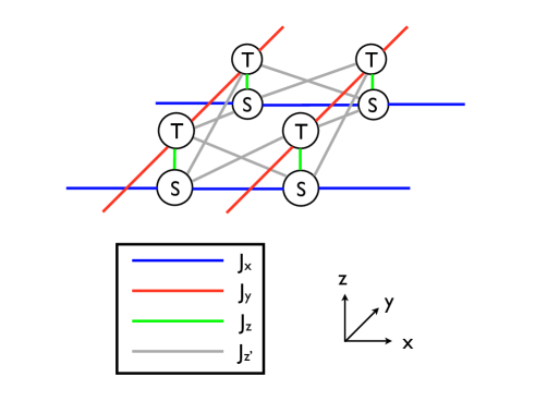
Figure 1: (Color online) The geometry of the interactions in the CICM for four sites is shown. This model is studied on an $L$ $\times$ $L$ square lattice with periodic boundary conditions (in the $\hat{x}$ and $\hat{y}$ directions) containing $N$ (= $L^{2}$) “S spins” and N “T spins” taking values $\pm 1$. There are $L$ parallel 1D chains of S spins in the $\hat{x}$ direction and $L$ parallel 1D chains of T spins in the $\hat{y}$ direction, illustrated by the blue ($J_{x}$) and red ($J_{y}$) lines, respectively. There is an interaction between an S and a T spin on the same site in the $\hat{z}$ direction ($J_{z}$) illustrated by the green lines. Finally, there is an interaction between nearest neighbor S and T spins ($J_{z^{\prime}}$) which is illustrated by the gray lines.

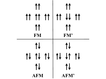
Figure 2: The four ordered phases found in the CICM are defined. Each pair of spins represents an S and a T spin on a single site (i.e. coupled by $J_{z}$). In the ferromagnetic (FM) phase, all S and T spins are aligned ferromagnetically. In the ferromagnetic prime (FM^′) phase, the S and T spins are aligned ferromagnetically on each site and antiferromagnetically along the S and T chains. In the antiferromagnetic (AFM) phase, the S and T spins are aligned antiferromagnetically on each site and ferromagnetically along the S and T chains. Finally, in the antiferromagnetic-prime (AFM^′) phase, the S and T spins are aligned antiferromagnetically on each site and also along the S and T chains. There is spin inversion symmetry in this model so flipping all of the spins in any of these phases does not change the phase.

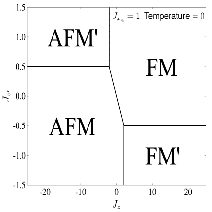
Figure 3: The phase diagram for the CICM with $J_{x,y}$=1 and T=0 in the $J_{z^{\prime}}$ versus $J_{z}$ parameter space is shown. The line separating the FM and AFM phases (where the internal energies are equal) is given by $J_{z^{\prime}}$=$-\frac{1}{4}J_{z}$. The AFM and AFM^′ phases are separated by $J_{z^{\prime}}=\frac{J_{x,y}}{2}=\frac{1}{2}$; the FM and FM^′ phases by $J_{z^{\prime}}=\frac{-J_{x,y}}{2}=\frac{-1}{2}$; the FM and AFM^′ phases by $J_{z}=-2J_{x,y}=-2$; and the AFM and FM^′ phases by $J_{z}=2J_{x,y}=2$. This phase diagram is consistent with the observation that for $J_{z}$ and $J_{z^{\prime}}$ both positive or both negative, there is no competition between phases. Additionally, the symmetry between FM and AFM and FM^′ and AFM^′ when switching the signs of $J_{z}$ and $J_{z^{\prime}}$ is evident.

The remainder of this paper is organized as follows. We begin our discussion of Eq. (1) via a mean field treatment. The resulting phase diagrams, as in the case of the BCM, will be shown to correctly predict certain qualitative features of the CICM such as the presence of ordered phases, effective Ising regimes in the large $|J_{z}|$ limit, and tricritical points. We then turn to a Monte Carlo (MC) approach which allows a more accurate quantitative determination of the phase diagram. We use the standard single-spin flip Metropolis MC algorithm, supplemented by some multiple-spin flips. The data are analyzed with standard numerical approaches, including the use of the Binder fourth order cumulant landau00 . The results show that there are four ordered phases, each of which becomes an effective Ising model in the large $|J_{z}|$ limit with unique effective couplings. Additionally, the presence of tricritical points is confirmed. In order to provide further corroboration for the nature of the phase transitions, we also employ the Wang-Landau algorithmwang01a ; wang01b ; landau02 to obtain the density of states and the behavior of canonical distributions as a function of temperature when passing through first and second order phase transitions. We find that this algorithm is particularly well suited for verifying the order of a phase transition and therefore the existence of tricritical points. Finally, we use finite-size scaling techniques to verify the universality class of the CICM.

III Mean Field Theory

We solve Eq. (1) by replacing the two spin interactions with a single spin coupled to a self-consistently determined average spin value

$$m_{1}\equiv<S_{r}>\hskip 72.26999ptm_{2}\equiv<T_{r}>.$$ (3)

In the case of the FM’ and AFM’ phases, these order parameters alternate in sign on the (bipartite) lattice.

The resulting implicit equations for the order parameters, $m_{FM}$=$m_{1}$=$m_{2}$ and $m_{AFM}$=$m_{1}$=$-m_{2}$ ($\beta=\frac{1}{T}$ and $k_{B}=1$),

$$m_{FM} =\frac{\sinh{(4\beta m_{FM}(J_{x,y}+2J_{z^{\prime}}))}}{\cosh{(4\beta m_{FM}(J_{x,y}+2J_{z^{\prime}}))}+e^{-2\beta J_{z}}}$$

$$m_{AFM} =\frac{\sinh{(4\beta m_{AFM}(J_{x,y}-2J_{z^{\prime}}))}}{\cosh{(4\beta m_{AFM}(J_{x,y}-2J_{z^{\prime}}))}+e^{2\beta J_{z}}}$$ (4)

are solved using Newton’s method. Equivalently, the mean field free energy of the CICM can be expanded in a power series in the order parameter for both the FM and AFM phases and the critical temperature for a second order phase transition determined by calculating the temperature where the coefficient of the quadratic term in the free energy expansion vanishes. The implicit equations for the FM and AFM second order critical lines are as follows.

$$T_{\text{C,FM}} =\frac{4(J_{x,y}+2J_{z^{\prime}})}{1+e^{\frac{-2J_{z}}{T_{\text{C,FM}}}}}$$

$$T_{\text{C,AFM}} =\frac{4(J_{x,y}-2J_{z^{\prime}})}{1+e^{\frac{2J_{z}}{T_{\text{C,AFM}}}}}.$$ (5)

Tricritical points are located by calculating the temperature at which the quartic coefficient in the expansion of the free energy vanishes.

$$T_{\text{tricritical, FM}} =\frac{-2}{\ln(2)}J_{z}$$

$$T_{\text{tricritical, AFM}} =\frac{2}{\ln(2)}J_{z}.$$ (6)

Combining this with the condition for intesecting the second order phase boundary, simple analytic expressions for the coordinates of the mean field tricritical points can be written down.

$$T_{\text{tricritical point, FM}} =\frac{4(J_{x,y}+2J_{z^{\prime}})}{3}$$

$$J_{\text{z,tricritical point, FM}} =\frac{-2\ln(2)(J_{x,y}+2J_{z^{\prime}})}{3}$$

$$T_{\text{tricritical point, AFM}} =\frac{4(J_{x,y}-2J_{z^{\prime}})}{3}$$

$$J_{\text{z,tricritical point, AFM}} =\frac{2\ln(2)(J_{x,y}-2J_{z^{\prime}})}{3}$$ (7)

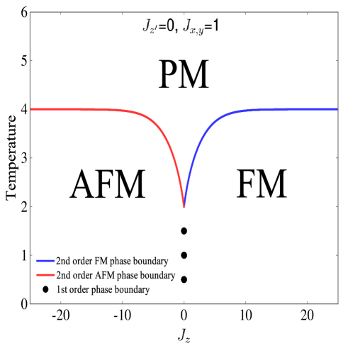
Figure 4: (Color online) The mean field theory phase diagram for $J_{z^{\prime}}=0$ and $J_{x,y}=1$ is shown. For these parameters, there is no tricritical point. For $J_{z}>$ 0, there is a second order phase transition between a low temperature FM phase and a high temperature PM phase. For $J_{z}$ $<$ 0, there is a second order phase transition between a low temperature AFM phase and a high temperature PM phase. Also, there is a vertical first order phase boundary between the FM and AFM phases at $J_{z}$= 0 which extends up to T=2, the MF critical temperature for the 1D Ising model. In the large, positive $J_{z}$ limit, this model becomes an effective 2D Ising model with $T_{C}=4(J_{x,y}+2J_{z^{\prime}})=4$. In the large, negative $J_{z}$ limit, this model also becomes an effective 2D Ising model with $T_{C}=4(J_{x,y}-2J_{z^{\prime}})=4$. The FM and AFM phase shapes are symmetric about $J_{z}$=0 only when $J_{z^{\prime}}$=0.

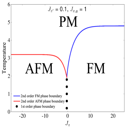
Figure 5: (Color online) The mean field theory phase diagram for $J_{z^{\prime}}=0.1$ and $J_{x,y}=1$ is shown. For these parameters, there is no tricritical point. For $J_{z}>-4J_{z^{\prime}}=-0.4$, there is a second order phase transition between a low temperature FM phase and a high temperature PM phase. For $J_{z}$ $<-4J_{z^{\prime}}=-0.4$, there is a second order phase transition between a low temperature AFM phase and a high temperature PM phase. Also, there is a vertical first order phase boundary between the FM and AFM phases at $J_{z}=-0.4$. In the large, positive $J_{z}$ limit, this model becomes an effective 2D Ising model with $T_{C}=4(J_{x,y}+2J_{z^{\prime}})=4.8$. In the large, negative $J_{z}$ limit, this model also becomes an effective 2D Ising model with $T_{C}=4(J_{x,y}-2J_{z^{\prime}})=3.2$. A positive $J_{z^{\prime}}$ shrinks the AFM phase and grows the FM phase as it is increased in magnitude, as evidenced by comparing with the phase diagram for $J_{z^{\prime}}=0$.

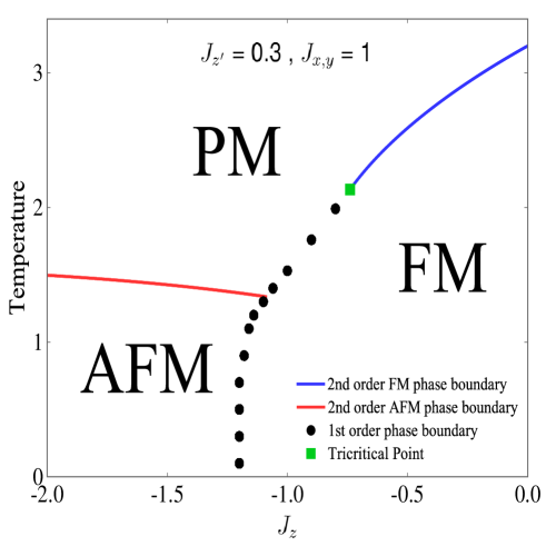
Figure 6: (Color online) The mean field theory phase diagram for $J_{z^{\prime}}=0.3$ and $J_{x,y}=1$ is shown. For $J_{z}$ $\gtrsim-0.7$, there is a second order phase transition between a low temperature FM phase and a high temperature PM phase. For $-1.1\lesssim$ $J_{z}$ $\lesssim-0.7$, there is a first order phase transition between a low temperature FM phase and a high temperature PM phase. This section of the phase diagram is separated from the previous section by the green square tricritical point (located at T = $\frac{32}{15}\approx 2.13$, $J_{z}$ = $\frac{-16\ln(2)}{15}\approx-0.74$). For $-1.2\lesssim$ $J_{z}$ $\lesssim-1.1$ there is a low temperature FM phase followed by a small higher temperature AFM phase and then, for higher temperatures, a disordered PM phase. For $J_{z}$ $\lesssim-1.2$ there is a second order phase boundary between a low temperature AFM phase and a high temperature PM phase. Additionally, there is an approximately vertical first order phase boundary between the FM and AFM phases at $J_{z}$ $=$ $-1.2$. This phase diagram is zoomed in relative to the other phase diagrams in order to show the details of the tricritical point and first order phase boundary.

To find the first order phase boundary once the tricritical point has been reached, simultaneous plots of the FM and AFM free energy were made and temperature or $J_{z}$ was incremented to find the point where the phase with the global minimum changes.

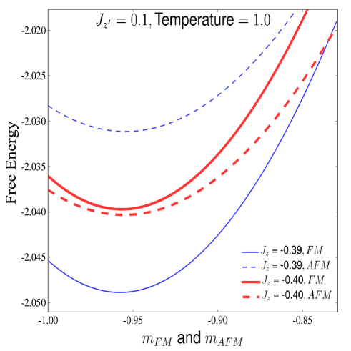
Figure 7: (Color online) A plot of the FM and AFM free energies at $J_{z^{\prime}}=0.1$ and T=1.0 is shown. For $J_{z}$=$-0.39$ the minimum of the FM free energy (thin blue solid curve) is lower than the minimum of the AFM free energy (thin blue dashed curve) and therefore, the system is in the FM phase. For $J_{z}$=$-0.40$ the minimum of the FM free energy (thick red solid curve) is greater than the minimum of AFM free energy (thick red dashed curve) and therefore the system is in the AFM phase. If the global minima were to be at m=0, the system is in the PM phase where the total magnetization is 0. This is the analysis used to determine all of the first order phase boundaries in the mean field theory phase diagrams.

For $J_{z^{\prime}}$ = 0, the mean field phase diagram (Fig. 4) shows no tricritical point. Clearly, $J_{z^{\prime}}$ is necessary for the onset of first order phase transitions. The AFM phase arises for $J_{z}<0$, as expected, since negative $J_{z}$ antiferromagnetically couples the $S$ and $T$ spins on shared sites. For $J_{z}>0$, the FM phase arises. The mean field phase boundary separating the FM and AFM phases at $T=0$ where thermal fluctuations are nonexistent agrees with the ground state phase diagram in Fig. 3. The MFT critical temperature is $T_{C}=2$ at $J_{z}$=0 and $J_{z^{\prime}}$=0, as expected since the CICM decouples into independent 1D Ising chains For large $|J_{z}|$, the $S$ and $T$ spin pairs on each site lose their independence due to the high energy cost of flipping only one of the spins in a pair. In this limit, the model becomes an effective 2D Ising model with $J_{\text{eff,FM}}=J_{x,y}+2J_{z^{\prime}}$ and $J_{\text{eff},AFM}=J_{x,y}-2J_{z^{\prime}}$ for positive and negative $J_{z}$, respectively. This leads to the limiting values $T_{C}=4$ for $|J_{z}|$ large in Fig. 4.

In fact, this single “locked spin” Ising regime in the large $|J_{z}|$ limit occurs for all four ordered phases. However, the effective couplings are different for each phase. In the large, negative $J_{z}$ limit, the AFM and AFM^′ phases have the following effective Ising couplings.

$$J_{\text{eff,AFM}} =J_{x,y}-2J_{z^{\prime}}$$

$$J_{\text{eff,AFM${}^{\prime}$}} =-J_{x,y}+2J_{z^{\prime}}$$ (8)

Meanwhile, in the large, positive $J_{z}$ limit, the FM and FM^′ phases have the following different effective Ising couplings.

$$J_{\text{eff,FM}} =J_{x,y}+2J_{z^{\prime}}$$

$$J_{\text{eff,FM${}^{\prime}$}} =-J_{x,y}-2J_{z^{\prime}}.$$ (9)

This behavior is similar to that of the Blume-Capel Model (BCM) which also approaches an Ising limit for large negative $\Delta$ which drives the density of vacancy sites $M_{i}=0$ to zero. However, our model does not approach the “vacant” lattice limit of the BCM at large positive $\Delta$, because even though $S_{i}=-T_{i}$ in the AFM and AFM^′ phases, the individual nonzero $S$ and $T$ moments still couple down their respective chains. It is interesting, therefore, that, as we shall see, the tricritical points which are driven by vacancies in the BCM are still present in the CICM.

When $J_{z^{\prime}}\neq 0$ the phase diagram loses its symmetry on changing the sign of $J_{z}$. As expected, for $J_{z^{\prime}}$=0.1 (Fig. 5), the AFM and FM phases meet at $J_{z}$=-4$J_{z^{\prime}}$=-0.4. Also, for large, negative $J_{z}$, $T_{c}$ = 4($J_{x,y}-2J_{z^{\prime}}$)=3.2 and for large, postive $J_{z}$, $T_{c}$ = 4($J_{x,y}+2J_{z^{\prime}}$)=4.8; as $J_{z^{\prime}}>0$ gets larger, the FM phase gets larger and the AFM phase shrinks. The phase diagram is reflected about $J_{z}$=0 for $J_{z^{\prime}}$=$-0.1$ (not shown): the AFM region expands and the FM region shrinks.

Most importantly, the value of $J_{z^{\prime}}$ determines whether or not there is a triciritcal point. For $J_{z^{\prime}}=0.0$ and $0.1$, there is no tricritical point and all thermally driven phase transitions between an ordered phase and the disordered phase are of second order. However, for $J_{z^{\prime}}$ = 0.3 (Fig. 6) there is a tricritical point. The thermally driven phase transition between the PM and the FM phase switches from second order to first order. The FM tricritical point emerges when $J_{z^{\prime}}$ $>$ $\frac{J_{x,y}}{6}$=$\frac{1}{6}$, a result which follows from a detailed analysis of Eq. (5) and Eq. (7).

IV Metropolis Monte Carlo

In order to achieve more accurate quantitative results, the Metropolis MC algorithm was implemented. We include moves which flip a single S spin, a single T spin, a row of S spins, a column of T spins, and an S and T spin simultaneously on a single site. What we will call one sweep alternates between the following five procedures: flipping every S spin ($N$ total flips), flipping every T spin ($N$ total flips), flipping every row of S spins ($L$ total flips), flipping every column of T spins ($L$ total flips), and flipping every S and T pair ($N$ total flips). To thermalize the lattice we perform $5\times 10^{5}$ such sweeps of the lattice (i.e. $10^{5}$ sweeps of each type). We then perform another $5\times 10^{5}$ sweeps of the lattice, making a measurement every 10 sweeps. Flipping multiple spins at a time helps the system to break out of metastable states and thereby makes the algorithm more efficient. For example, if $J_{z}$ is large and positive and a pair of S and T spins both have values of +1, the probability of both spins changing to $-1$ is very small if only single spin flips are allowed. This is because of the large increase in energy that would come from trying to change the value of one of them first (i.e. making them align antiferromagnetically).

In order to calculate the critical temperatures, the Binder fourth order cumulant,

$$U_{L}=1-\frac{<m^{4}>}{3<m^{2}>^{2}}$$ (10)

where m is either $m_{\rm FM}$, $m_{\rm AFM}$, $m_{\rm FM^{\prime}}$, or $m_{\rm AFM^{\prime}}$ is calculated as a function of temperature for various lattice sizes, $L$. Curves for different lattice sizes have a common intersection point at the critical temperature ($T_{C}$), regardless of the order of the transition vollmayr93 . Additionally, the behavior of the Binder cumulant away from the crossing at $T_{C}$ can be used to distinguish between first and second order phase transitions. For second order phase transitions, $U_{L}$ approaches the value $U_{L}=\frac{2}{3}$ as the temperature approaches zero. For temperatures above the critical temperature, $U_{L}$ approaches $U_{L}=0$, all the while staying between these two values. For first order phase transitions, the Binder cumulant has the same limit values but, above the transition temperature, it develops a minimum that dips below 0 and which gets deeper for larger lattice sizes vollmayr93 .

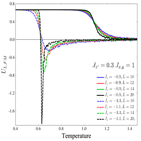
Figure 8: (Color online) The Binder fourth order cumulants for various lattice sizes and for a second order phase transition (solid lines) at $J_{z}=-0.9$ and a first order phase transition (dashed lines) at $J_{z}=-1.1$. A minimum below $U_{L,{\rm FM}}$=0, which gets deeper as the lattice size increases, is a signature of a first order phase transition. The curves intersect at a single critical temperature in both cases. In both cases, at lower temperatures than the crossing, the order of the curves from top to bottom are $L$=20, $L$=14, $L$=12, and finally $L$=10. $U_{L}$ was used to determine all of the critical points in the MC phase diagrams.

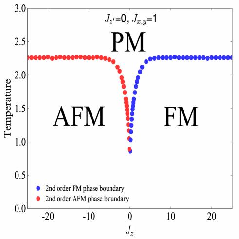
Figure 9: (Color online) The MC-derived phase diagram for $J_{z^{\prime}}=0$ and $J_{x,y}=1$ is shown. For $J_{z}>$ 0, there is a second order phase boundary separating a low temperature FM phase from a high temperature PM phase. The critical temperature increases as $J_{z}$ increases and saturates at $T_{C}\approx 2.269(J_{x,y}+2J_{z^{\prime}})=2.269$. For $J_{z}<$ 0, there is a second order phase boundary separating a low temperature AFM phase from a high temperature PM phase. Similarly, the critical temperature increases as $J_{z}$ decreases until it saturates at with $T_{C}\approx 2.269(J_{x,y}-2J_{z^{\prime}})=2.269$. This phase diagram is qualitatively similar to the MFT phase diagram with the same parameters, particularly in its lack of a tricritical point. As expected, the critical temperatures were overestimated in MFT.

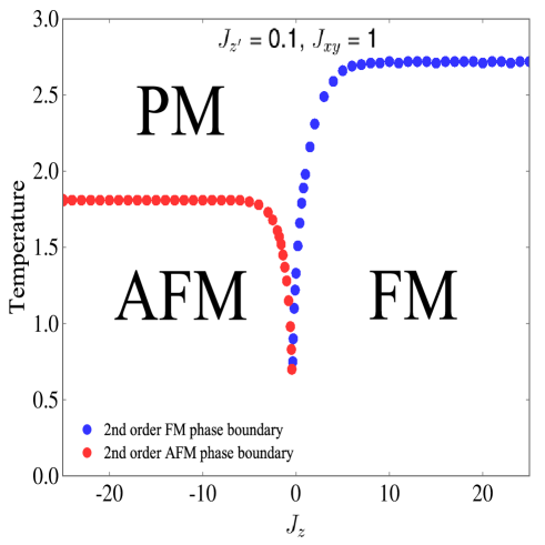
Figure 10: (Color online) Same as Fig. 9 except $J_{z^{\prime}}=0.1$. The phase diagram is qualitatively similar to the result of MFT, particularly in its lack of a tricritical point.

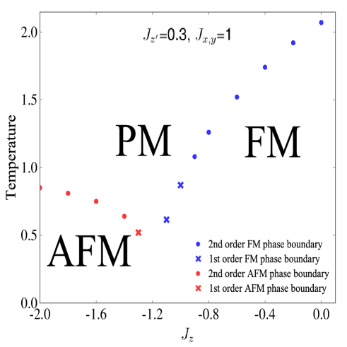
Figure 11: (Color online) Same as Fig. 9 except $J_{z^{\prime}}=0.3.$ The phase diagram is qualitatively similar to the result of MFT in most regards. However, MC finds that a tricritical point, which is present only on the FM side in MFT, is also present on the AFM phase boundary.

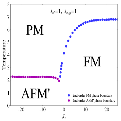
Figure 12: (Color online) Same as Fig. 9 except $J_{z^{\prime}}=1.0.$ As for $J_{z^{\prime}}=0.0$ and $0.1$, there is no tricritical point, which thus appear to be restricted to intermediate $J_{z^{\prime}}\approx 0.3$.

For $J_{z^{\prime}}$=0, the MC phase diagram of Fig. 9 has the same qualitative features as the mean field phase diagram. In both cases there are two ordered phases at low temperatures, FM and AFM, and a PM phase at high temperatures. The AFM and FM phases meet, as expected, at $J_{z}$=$-4J_{z^{\prime}}=$0. Additionally, the MC phase diagram also contains the expected Ising regimes at large $|J_{z}|$, that is, $T_{C}\approx 2.269J_{\text{eff}}$ onsager44 . For large positive $J_{z}$ this leads to $T_{C}$ $\approx$ 2.269 ($J_{x,y}+2J_{z^{\prime}})=2.269$ and for large negative $J_{z}$, $T_{C}$ $\approx$ 2.269 ($J_{x,y}-2J_{z^{\prime}})=2.269$. We can estimate the error bars on the MC simulations by comparing how close the MC data is to the exact value in the Ising regime. This leads to error bars on the critical temperatures of $\pm 0.02$. Another way of quantifying the uncertainty in the values of the critical temperatures is to estimate the “spread” in the crossings of the fourth order Binder cumulants for the various lattice sizes, since the crossings are not perfectly sharp. This measure also leads to error bars on the critical temperatures of $\pm 0.02$.

Similarly, for $J_{z^{\prime}}$=0.1 (Fig. 10) the MC phase diagram qualitatively agrees with the mean field theory phase diagram. There is no tricritical point in either the mean field theory or MC phase diagrams and the FM and AFM phases meet at $J_{z}$=$-4J_{z^{\prime}}=-0.4$ in both cases. For large positive $J_{z}$, we expect $T_{C}$ $\approx$ 2.269 ($J_{x,y}+2J_{z^{\prime}}$) $\approx$ 2.723 and for large negative $J_{z}$, we expect $T_{C}$ $\approx$ 2.269 ($J_{x,y}-2J_{z^{\prime}}$) $\approx$ 1.815, which agrees with the MC data.

Fig. 11 shows MC results for $J_{z^{\prime}}$=0.3. The FM and AFM phases meet at $J_{z}$=-4$J_{z^{\prime}}=-1.2$, as in the MF phase diagram, and there is a FM tricritical point at $J_{z}=-0.9(1)$. One important qualitiative difference between the MF and MC phase diagrams for $J_{z^{\prime}}$=0.3 is that there is also an AFM tricritical point in the MC phase diagram. The MF phase diagram also has a small parameter window for $-1.2\lesssim$ $J_{z}$ $\lesssim-1.1$ where raising the temperature from the FM phase results in passage through an intermediate AFM phase before the disordered high temperature regime is reached. We do not observe this in the MC data.

Finally, in Fig. 12 the phase diagram for $J_{z^{\prime}}$=1.0 is shown. The FM and AFM’ phases meet at $J_{z}=-2$, as expected from the ground state phase diagram. There is no tricritical point for this value of $J_{z^{\prime}}$ which shows that there is some intermediate range between $J_{z^{\prime}}$=0.1 and $J_{z^{\prime}}$=1.0 where tricritical points are present.

V Wang-Landau Sampling

While the Metropolis MC algorithm is the most widely used method of numerically calculating the thermodynamic properites of classical spin models, there exist more sophisticated alternatives. One is Wang-Landau sampling (WLS). In WLS, the density of states (DOS) is determined using a MC procedure. From the DOS, all of the desired thermodynamic properties can be calculated. The major advantage of WLS is that the DOS is independent of temperature so that only one simulation is needed to calculate thermodyanamic quantities at any temperature. Additionally, the DOS can be used to calculate the unnormalized canonical distribution, $P(E)$,

$$P(E)\propto g(E)\,e^{-\beta E}$$ (11)

for various temperatures from one simulation. This distribution is another useful tool for distinguishing between first and second order phase transitions as it has distinct behavior in the two cases. For second order phase transitions, the canonical distribution is always a single peaked distribution which shifts its average value as the temperature changes. For first order phase transitions, the canonical distribution is similarly a single peaked distribution at temperatures well above and below the phase boundary. However, it develops a characteristic double peaked structure near the transition temperature due to phase coexistence. The peaks are of equal height at the transition temperature challa86 .

This doubly peaked canonical distribution was found for our model as is shown in Fig. 13, providing additional confirmation for the existence of the first order phase transition. For $J_{z}=-1.1$ and $J_{z^{\prime}}$=0.3, the peaks were found to be of equal height at $T_{C}=$ 0.6173(2). The Metropolis MC data with the same parameters gave $T_{C}=$ 0.615(5), which envelopes the Wang-Landau value. This procedure confirmed all three first order phase transition data points ($J_{z}$=$-1.3,-1.1,-1.0$) in the $J_{z^{\prime}}$=0.3 MC phase diagram.

A clear and comprehensive detailing of the WLS algorithm can be found in the literature wang01a ; wang01b ; landau02 . However, a few specific details of our simulations are worthy of mention. The energies in our Wang-Landau simulation were not binned. In other words, every unique configuration energy has it’s own data point in the density of states. Also, windows were not used in the sampling. The entire energy spectrum shown was sampled in one simulation. Every 10,000 $\times$ 2$N$ spin flips, the histogram is checked for flatness. The flatness criterion used is that no individual energy is visited less than 80 percent of the average number of visits over all energies. When this criterion is achieved, the modification factor, f, which was initialized to f=e, is reduced ($f_{i+1}=\sqrt{f_{i}}$), the histogram H(E) is reset to zero and the process of spin flipping is continued. This algorithm continued until f was less than $e^{10^{-6}}$ at which time the density of states converged to our desired level of accuracy. The Wang Landau algorithm calculates the relative density of states and, therefore, the density of states was normalized as follows,

$$\ln({g_{\text{normalized}}(E_{i})})=\ln({g_{\text{unnormalized}}(E_{i})})\\ -\ln({g_{\text{unnormalized}}(E_{GS})})+\ln({g_{\text{normalized}}(E_{GS})})$$ (12)

For the CICM, there are two ground states due to it’s spin inversion symmetry.

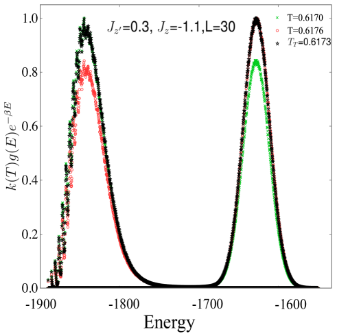
Figure 13: (Color online) The canonical distributions for three temperatures around a first order phase boundary are shown (with $J_{z}$ = $-1.1$ and $J_{z^{\prime}}$=0.3). The characteristic double peak behavior due to phase coexistence is clear. At the transition temperature ($T_{T}$) (black data), the two peaks are of equal height. The canonical distributions were normalized by the constant k(T) such that the maximum height of the distribution is equal to 1. This simulation was performed on a size $L$=30 lattice.

VI Critical exponents

The CICM consists of Ising spins on one dimensional chains with interchain couplings that connect the system into a two-dimensional lattice and therefore, we expect it to belong to the two-dimensional Ising universality class where the magnetization critical exponent $\beta=\frac{1}{8}$, the correlation length critical exponent $\nu=1$, and the magnetic susceptibility critical exponent $\gamma=\frac{7}{4}$. To verify this universality class for the CICM (away from the tricritical point) a finite size scaling analysis was performed. Plots of ($L^{\frac{2\beta}{\nu}}$ $<m^{2}_{FM}(t)>$) vs. ($L^{\frac{1}{\nu}}$t) and ($L^{\frac{-\gamma}{\nu}}$ $<\chi_{L}(t)>$) vs. ($L^{\frac{1}{\nu}}$t) for various values of $L$ will collapse onto a single curve for the correct values of the exponents $\beta$, $\nu$, and $\gamma$ newman99 . We measured $<m_{FM}^{2}>$ and $<\chi_{L}>$ as a function of temperature for the CICM with $J_{z}$=25 and $J_{z^{\prime}}$=0.3. For these parameters, $T_{C}$ = 3.63. This was used to define the reduced temperature t = $\frac{T-T_{C}}{T_{C}}$. Fig. 14 and Fig. 15 show the results of this analysis. The data collapses nicely over a broad range of temperatures. This provides a satisfying consistency check to our expectation of the universality class of the CICM.

Precisely at a tricritical point, the critical exponents are known to take on different tricritical values landau00 . We attempted to measure the tricritical exponents at the tricritical point in our model but this proved to require a level of precision beyond the scope of our work. However, we did find that when applying the same finite size scaling analysis that is detailed in the previous paragraph, including using the same two-dimensional Ising exponents, to a tricritical point in our model ($J_{z}$=-0.9 and $J_{z^{\prime}}$=0.3), there was a significant decrease in the degree to which the data “collapsed.” Although inconclusive, this finding is consistent with our expectation that there will be a change in exponents at the tricritical point.

Finally, the critical Binder cumulant, U* is the value of the Binder cumulant at the critical temperature in the thermodynamic limit. For the 2D square Ising model it has been shown that U*=0.61069… Kamieniarz . For $J_{z}$=25 and $J_{z^{\prime}}$=0.3 in the CICM, our data shows that U* is somewhere between 0.605 and 0.615, consistent with the known value for 2D Ising universality. At $J_{z}$=-0.9 and $J_{z^{\prime}}$=0.3 (approximate location of a tricritical point) our data has a larger spread of possible U* values although it is clearly less than 0.61069. U* at the tricritical point is in the range 0.50 to 0.55. We also measured U* at the tricritical point of the 2D Blume-Capel model and a similar range of values was found, providing some evidence in favor of 2D tricritical Ising universality.

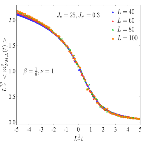
Figure 14: (Color online) The data collapse of ($L^{\frac{2\beta}{\nu}}$ $<m^{2}_{FM}(t)>$) vs. ($L^{\frac{1}{\nu}}$t) for $L$ = 40, 60, 80, and 100 using the two-dimensional Ising universality class exponents is shown.

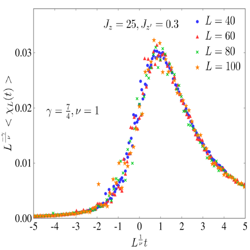
Figure 15: (Color online) The data collapse of ($L^{\frac{-\gamma}{\nu}}$ $<\chi_{L}(t)>$) vs. ($L^{\frac{1}{\nu}}$t) for $L$ = 40, 60, 80, and 100 using the two-dimensional Ising universality class exponents is shown.

VII Conclusions

Using a combination of mean field theory, Metropolis MC, and Wang-Landau simulations, we have explored an Ising-like model on a lattice composed of a 1D$\times$1D collection of coupled chains. As is well known, 1D Ising chains with short range interactions do not exhibit finite temperature ordered phases. However, interchain couplings connect the chains into a 2D framework which shows multiple ordered phases at finite temperatures. The phase transitions between the ordered and disordered phases can be of first or second order as evidenced by the behavior of the Binder fourth order cumulants and the canonical distributions. The existence of tricritical points in the phase diagram depends on the value of $J_{z^{\prime}}$. According to the MC simulations, for $J_{z^{\prime}}$=0.1 and 1.0, there are no tricritical points but for intermediate $J_{z^{\prime}}$=0.3, there are tricritical points.

It would be interesting to see if the Nb₁₂O₂₉ materials can be tuned between first and second order transitions by varying pressure, doping or other parameters, thus giving rise to novel realizations of tricritical systems.

In some materials which exhibit this 1D$\times$1D geometry, the quantum mechanical nature of the degrees of freedom may be crucial to the observed phenomena. For example, in the optical lattice case, the focus is on the occurrence of Bose-Einstein condensation at finite momentum, and in a pattern of orbitals which alternates as $p_{x}\pm ip_{y}$ on the two sublattices. Our work shows that even at the classical level, these crossed-chains systems exhibit complex phase-transitions and crossovers. Future work could address the additional non-trivial physics which arises when the phase transitions are driven to $T=0$, giving rise to exotic quantum phase transitions. Additional future work could study the critical and tricritical exponents of this model with greater precision and breadth.

TC and RTS were supported by Department of Energy grant DE-SC0014671. The work of RRPS is supported by the US National Science Foundation grant number DMR-1306048.

References

- (1) “Equilibrium Statistical Mechanics of Lattice Models,” D. Lavis, Springer, Netherlands (2015).
- (2) “Critical properties of site- and bond-diluted Ising ferromagnets,” J.M.Yeomans, R.B. Stinchcombe, Journal of Physics C: Solid State Physics 12, 2 (1979).
- (3) “Critical Phenomena on Fractal Lattices,” Y. Gefen, B. B. Mandelbrot, and A. Aharony, Phys. Rev. Lett. 45, 855, (1980).
- (4) “Ising Model with a Long-Range Interaction in the Presence of Residual Short-Range Interactions,” George A. Baker, Jr., Phys. Rev. 130, 1406 (1963).
- (5) “Ising Chain with Competing Interactions,” John F. Nagle, Phys. Rev. A 2, 2124 (1970).
- (6) “Critical Behavior of Ising Models with Random Long-Range Interactions,” R.T. Scalettar, Physica A 170, 282 (1991).
- (7) “Exact solution of Ising model on a small-world network,” J. Viana Lopes, Yu. G. Pogorelov, and J. M. B. Lopes dos Santos, Phys. Rev. E 70, 026112 (2004).
- (8) “Small-world phenomena in physics: the Ising model,” M. Gitterman, J. Phys. A: Math. Gen. 33, 8373 (2000).
- (9) “Organometallic-like localization of 4d-derived spins in an inorganic conducting niobium suboxide,” K.-W. Lee and W. E. Pickett, Phys. Rev. B 91, 195152 (2015).
- (10) “Antiferromagnetism and metallic conductivity in Nb12O29,” R.J. Cava, B. Batlogg, J.J. Krajekski, P. Gammel, H.F. Poulsen, W.F. Peck, Jr., and L.W. Rupp, Jr., Nature 350, 598 (1991).
- (11) “Nanometer structural columns and frustration of magnetic ordering in Nb12O29,” E.N. Andersen, T. Klimczuk, V.L. Miller, H.W. Zandbergen, and R.J. Cava, Phys. Rev. B 72, 033413 (2005).
- (12) “Optical Lattices,” M. Greiner and S. Fölling, Nature 453, 736 (2008).
- (13) “Multiflavor bosonic Hubbard models in the first excited Bloch band of an optical lattice,” A. Isacsson and S.M. Girvin, Phys. Rev. A 72, 053604 (2005).
- (14) “Unconventional Bose-Einstein Condensation Beyond The ”No-Node” Theorem,” C. Wu, Mod. Phys. Lett. B 23, 1 (2009).
- (15) “Atomic matter of nonzero-momentum Bose-Einstein condensation and orbital current order,” W. V. Liu, and C. Wu, Phys. Rev. A 74, 013607 (2006).
- (16) “Exotic phases of -band bosons in interaction,” F. Hébert, Zi Cai, V.G. Rousseau, Congjun Wu, R.T. Scalettar, and G.G. Batrouni, Phys. Rev. B 87, 224505 (2013).
- (17) “Exact Results for Itinerant Ferromagnetism in Multiorbital Systems on Square and Cubic Lattices,” Yi Li, Elliott H. Lieb, and Congjun Wu, Phys. Rev. Lett. 112, 217201 (2014).
- (18) “Theory of the First-Order Magnetic Phase Change in ,” M. Blume, Phys. Rev. 141, 517 (1966).
- (19) “On the possibility of first-order phase transitions in Ising systems of triplet ions with zero-field splitting,” H.W. Capel, Physica 32, 966 (1966).
- (20) “A Guide to Monte Carlo Simulations in Statistical Physics,” D.P. Landau and K. Binder, Cambridge University Press (2000).
- (21) “Efficient, Multiple-Range Random Walk Algorithm to Calculate the Density of States,” F. Wang and D.P. Landau, Phys. Rev. Lett. 86, 2050 (2001).
- (22) “Determining the density of states for classical statistical models: A random walk algorithm to produce a flat histogram,” F. Wang and D.P. Landau, Phys. Rev. E 64, 056101 (2001).
- (23) “Determining the density of states for classical statistical models by a flat-histogram random walk,” D.P. Landau and F. Wang, Comput. Phys. Commun. 147, 674 (2002).
- (24) “Finite size effects at thermally-driven first order phase transitions: A phenomenological theory of the order parameter distribution,” K. Vollmayr, J.D. Reger, M. Scheucher, and K. Binder, Z. Phys. B 91, 113-125 (1993).
- (25) “Crystal Statistics. I. A Two-Dimensional Model with an Order-Disorder Transition,” Lars Onsager, Phys. Rev. 65, 117 (1944).
- (26) “Finite-size effects at temperature-driven first-order transitions,” M. S. S. Challa, D. P. Landau, and K. Binder, Phys. Rev. B 34, 1841 (1986).
- (27) “Monte Carlo Methods in Statistical Physics,” Newman and Barkema, Claredon Press (1999).
- (28) “Exact Critical Point and Critical Exponents of O(n) Models in Two Dimensions,” Bernard Nienhuis, Phys. Rev. Lett. 49, 1062, (1982).
- (29) “Universal ratio of magnetization moments in two-dimensional Ising models” G. Kamieniarz and H.W.J. Blote, J. Phys. A: Math. Gen. 26 201 (1993).