A Formal, Resource Consumption-Preserving Translation of Actors to Haskell

Abstract

We present a formal translation of an actor-based language with cooperative scheduling to the functional language Haskell. The translation is proven correct with respect to a formal semantics of the source language and a high-level operational semantics of the target, i.e. a subset of Haskell. The main correctness theorem is expressed in terms of a simulation relation between the operational semantics of actor programs and their translation. This allows us to then prove that the resource consumption is preserved over this translation, as we establish an equivalence of the cost of the original and Haskell-translated execution traces.

1 Introduction

Abstract Behavioural Specification (ABS) [9] is a formally-defined language for modeling actor-based programs. An actor program consists of computing entities called actors, each with a private state, and thread of control. Actors can communicate by exchanging messages asynchronously, i.e. without waiting for message delivery/reply. In ABS, the notion of actor corresponds to the active object, where objects are the concurrency units, i.e. each object conceptually has a dedicated thread of execution. Communication is based on asynchronous method calls where the caller object does not wait for the callee to reply with the method’s return value. Instead, the object can later use a future variable [8, 5] to extract the result of the asynchronous method. Each asynchronous method call adds a new process to the callee object’s process queue. ABS supports cooperative scheduling, which means that inside an object, the active process can decide to explicitly suspend its execution so as to allow another process from the queue to execute. This way, the interleaving of processes inside an active object is textually controlled by the programmer, similar to coroutines [10]. However, flexible and state-dependent interleaving is still supported: in particular, a process may suspend its execution waiting for a reply to a method call.

Whereas ABS has successfully been used to model [19], analyze [2], and verify [9] actor programs, the “real” execution of such programs has been a struggle, attributed to the fact that implementing cooperative scheduling efficiently can be hard (common languages as Java and C++ have to resort to instrumentation techniques, e.g. fibers [16]). This led to the creation of numerous ABS backends with different cooperative scheduling implementations: ABS$\rightarrow$Maude using an interpreter and term rewriting, ABS$\rightarrow$Java using heavyweight threads and manual stack management, ABS$\rightarrow$Erlang using lightweight threads and thread parking, ABS$\rightarrow$Haskell using lightweight threads and continuations.

The overall contribution of this paper is a formal, resource-consumption preserving translation of the concurrency subset of the ABS language into Haskell, given as an adaptation of the canonical ABS$\rightarrow$Haskell backend [4]. We opted for the Haskell backend relying on the hypothesis that Haskell serves as a better middleground between execution speed and most importantly semantic correctness. The translation is based on compiling ABS methods into Haskell functions with continuations—similar transformations have been performed in the actor-based Erlang language wrt. rewriting systems [14, 18] and rewriting logic [13], in the translation of ABS to Prolog [3] and a subset of ABS to Scala [11]. However, what is unique in our translation and constitutes our main contribution, is that the translation is resource preserving as we prove in two steps:

• Soundness. We provide a formal statement of the soundness of this translation of ABS into Haskell which is expressed in terms of a simulation relation between the operational ABS semantics and the semantics of the generated Haskell code. The soundness claim ensures that every Haskell derivation has an equivalent one in ABS. However, since for efficiency reasons, the translation fixes a selection order between the objects and the processes within each object, we do not have a completeness result.

• Resource-preservation. As a corollary we have that the transformation preserves the resource consumption, i.e., the cost of the Haskell-translated program is the same as the original ABS program wrt. any cost model that assigns a cost to each ABS instruction, since both programs execute the same trace of ABS instructions. This result allows us to ensure that upper bounds on the resource consumption obtained by the analysis of the original ABS program are preserved during compilation and are thus valid bounds for the Haskell-translated program as well.

In Section 2 we specify the syntax of the source language and detail its operational semantics. Section 3 describes our target language and defines the compilation process. We present the correctness and resource preservation results in Section 4, as well as the intermediate semantics used in this process. In Section 5 we show that the runtime environment does not introduce any significant overhead when executing ABS instructions, and show that the upper bounds obtained by the cost analysis are sound. Finally, Section 6 contains the conclusions and future work. Complete proofs of the theoretical results can be found at http://gpd.sip.ucm.es/enrique/publications/lopstr16_ext.pdf.

2 Source language

$\begin{array}[]{ll}S::=&\ x\texttt{:=}E~{}|~{}f\texttt{:=}x\texttt{!}m(\bar{y})\\ &|~{}\mathtt{await}\ f~{}|~{}\mathtt{skip}~{}|~{}\mathtt{return}\ z\\ &|~{}S_{1}\mathtt{;}S_{2}~{}|~{}\mathtt{if}\ B\ \{S\}\ \mathtt{else}\ \{S\}\\ &|~{}\mathtt{while}\ B\ \{S\}\\ E::=&\ V~{}|~{}\mathtt{new}~{}|~{}f\mathtt{.get}~{}|~{}m(\bar{y})\\ V::=&\ x~{}|~{}r~{}|~{}I\\ B::=&\ B\land B~{}|~{}B\lor B~{}|~{}\lnot B~{}|~{}V\equiv V\\ D::=&\ m(\bar{r})\{\;S\;\}\\ P::=&\ \overline{D}~{}:~{}\mathtt{main}()\{\;S\;\}\end{array}$

⬇

1main() {

2 node1 = new;

3 node2 = new;

4 f1 = node1!map(v₁);

5 f2 = node2!map(v₂);

6 await f1;

7 await f2;

8 r1 = f1.get;

⬇

9 r2 = f2.get;

10 r = reduce(r1,r2);

11 return r; }

12

13map(v) {

14 ... }

15reduce(v1,v2) {

16 ... }

Figure 1: (a) syntax of source language (b) a simplified MapReduce task in ABS

Our language is based on ABS [9], a statically-typed, actor-based language with a purely-functional core (ADTs, functions, parametric polymorphism) and an object-based imperative layer: objects with private-only attributes, and interfaces that serve as types to the objects. ABS extends the OO paradigm with support for asynchronous method calls; each call results in a new future (placeholder for the method’s result) returned to the caller-object, and a new process (stored in the callee-object’s process queue) which runs the method’s activation. The active process inside an object (only one at any given time) may decide to explicitly suspend its execution so as to allow another process from the same queue to execute.

In this paper, we simplify ABS to its subset that concerns the concurrent interaction of processes (inside and between objects), so as to focus solely on the more challenging part of proving correctness of the cooperative concurrency. In other words, the ABS language is stripped of its functional core, local variables, object groups [15] and types (we assume the input programs are well-typed w.r.t ABS type-system). The formal syntax of the statements $S$ of the subset is shown in Fig. 1(a). Values in our subset are references (object or futures) and integer numbers; values can be stored in method’s formal parameters or attributes. We syntactically distinguish between method parameters $r$ and attributes. The attributes are further distinguished for the values they hold: attributes holding object references or integer values (denoted by $x,y,z\ldots$), and future attributes holding future references (denoted by $f$). An assignment $f$:=$x$!$m(\bar{y})$ stores to the future attribute $f$ a new future reference returned by asynchronously calling the method $m$ on the object attribute $x$ passing as arguments the values of object attributes $\bar{y}$. An assignment $x$:=$E$ stores to an object attribute the result of executing the right-hand side $E$. A right-hand side can be the value of a method parameter $r$, an attribute $x$, an integer expression $I$ (an integer value, addition, subtraction, etc.), a reference to a new object new, the result of a synchronous same-object method call $m(\bar{y})$, or the result of an asynchronous method call $f$.get stored in the future attribute $f$. A call to $f$.get will block the object and all its processes until the result of the asynchronous call is ready. The statement $\mathtt{await}~{}f$ may be used (usually before calling $f$.get ) to instead release the current process until the result of $f$ has been computed, allowing another same-object process to execute. Sequential composition of two statements $S_{1}$ and $S_{2}$ is denoted by $S_{1};S_{2}$. The Boolean condition $B$ in the if and while statement is a Boolean combination of reference equality between values of attributes. Again, note that, we assume expressions to be well-typed: integer expressions cannot contain futures or object references and boolean equality is between same-type values. The statement $\mathtt{return}\;z$ returns the value of the attribute $z$ both in synchronous and asynchronous method calls. A method declaration $D$ maps a method’s name and formal parameters to a statement $S$ (method body). We consider that every method has one return and it is the final statement. Finally, a program $P$ is a set of method declarations $\bar{D}$ and a special method main that has no formal parameters and acts as the program’s entry point.

The program of Fig. 1(b) shows a basic version of a MapReduce task [7] implemented using actors in ABS. For clarity the example uses only two map nodes and a single reduce computation performed in the controller node (the actor running main). First the controller creates two objects node1 and node2 (L2–L3), and invokes asynchronously map with different values v₁ and v₂ (L4–L5). In MapReduce, all map invocations must finish before executing the reduce phase: therefore, the await instructions in L6–L7 wait for the termination of the two calls to map, releasing the processor so that any other process in the same object of main can execute. Once they have finished, the get statements in L8-L9 obtain the results from the futures f1 and f2. Although get statements block the object (in this case main) and all of its processes until the result is ready, this does not occur in our example because the preceding awaits assure the result is available. Finally, L10 contains a synchronous-method self call to reduce that combines the partial results from the map phase.

2.1 Operational semantics

$$\inference[(\textsc{Assign})]{\mathtt{getVal}({h(n)},{V})=v&h^{\prime}=h[(n)(x)\mapsto v)]}{\langle n:(\texttt{x:=}V;S,l)\cdot Q,h\rangle\rightarrow\langle n:(S,l)\cdot Q,h^{\prime}\rangle}$$

$$\inference[(\textsc{New})]{h(\mathit{count})=m&h^{\prime}=h[(n)(x)\mapsto m,(m)\mapsto\epsilon,\mathit{count}\mapsto m+1]}{\langle n:(\texttt{x:=new};S,l)\cdot Q,h\rangle\rightarrow\langle n:(S,l)\cdot Q,h^{\prime}\rangle}$$

$$\inference[(\textsc{Get})]{h(h(n)(f))\neq\bot&h^{\prime}=h[(n)(x)\mapsto h(h(n)(f))]\\ }{\langle n:(\texttt{x:=f.get};S,l)\cdot Q,h\rangle\rightarrow\langle n:(S,l)\cdot Q,h^{\prime}\rangle}$$

$$\inference[(\textsc{Await I})]{h(h(n)(f))\neq\bot\\ }{\langle n:(\texttt{await f};S,l)\cdot Q,h\rangle\rightarrow\langle n:(S,l)\cdot Q,h\rangle}$$

$$\inference[(\textsc{Await II})]{h(h(n)(f))=\bot\\ }{\langle n:(\texttt{await f};S,l)\cdot Q,h\rangle\rightarrow\langle n:Q\cdot(\texttt{await f};S,l),h\rangle}$$

$$\inference[(\textsc{Async})]{h(n)(x)=d&h(\mathit{count})=l^{\prime}\bar{v}=h(n)(\bar{z})\\ h^{\prime}=h[(n)(f)\mapsto l^{\prime},(l^{\prime})\mapsto\bot,\mathit{count}\mapsto l^{\prime}+1]}{\langle n:(\texttt{f:=x!m($\bar{z}$)};S,l)\cdot Q,h\rangle\stackrel{{\scriptstyle d.m(l^{\prime},\bar{v})}}{{\longrightarrow}}\langle n:(S,l)\cdot Q,h^{\prime}\rangle}$$

$$\inference[(\textsc{Sync})]{(m(\bar{w})\mapsto S_{m})\in D&\tau=[\bar{w}\mapsto h(n)(\bar{z})]S^{\prime}=\widehat{(S_{m}\tau)}^{x}}{\langle n:(\texttt{x:=m($\bar{z}$)};S,l)\cdot Q,h\rangle\rightarrow\langle n:(S^{\prime};S,l)\cdot Q,h\rangle}$$

$$\inference[(\textsc{Return${}_{A}$})]{h^{\prime}=h[(l)\mapsto h(n)(x)]}{\langle n:(\texttt{return}^{*}\texttt{x};S,l)\cdot Q,h\rangle\rightarrow\langle n:Q,h^{\prime}\rangle}$$

$$\inference[(\textsc{Return${}_{S}$})]{h^{\prime}=h[(n)(z)\mapsto h(n)(x)]}{\langle n:(\texttt{return}^{z}~{}\texttt{x};S,l)\cdot Q,h\rangle\rightarrow\langle n:(S,l)\cdot Q,h^{\prime}\rangle}$$

Figure 2: Operational semantics: Local rules

In order to describe the operational semantics of the language defined above we first introduce the following concepts and assumptions. The values considered in this paper are in the ${\it Int}$ set: integer constants and dynamically generated references to objects and futures. We denote by $\Sigma={\it IVar}\rightarrow{\it Int}$ the set of assignments of values to the instance variables (of an object), with typical element $\sigma$ and empty element $\epsilon$. A closure consists of a statement $S$ obtained by replacing its free variables by actual values (note that variables are introduced as method parameters and can only appear in $E$) and a future reference, represented by an integer, for storing the return value. By $S\tau$, where $\tau\in{\it LVar}\rightarrow{\it Int}$, we denote the instantiation obtained from $S$ by replacing each variable $x$ in $S$ by $\tau(x)$. Finally, we represent the global heap $h$ by a triple $(n,h_{1},h_{2})$ consisting of a natural number $n$ and partial functions (with finite disjoint domains) $h_{1}:{\it Int}\rightarrow\Sigma$ and $h_{2}:{\it Int}\rightarrow{\it Int}_{\bot}$, where ${\it Int}_{\bot}={\it Int}\cup\{\bot\}$ ($\bot$ is used to denote “undefined”). The number $n$ is used to generate references to new objects and futures. The function $h_{1}$ specifies for each existing object, i.e., a number $n$ such $h_{1}(n)$ is defined, its local state. The function $h_{2}$ specifies for each existing future reference, i.e., a number $n$ such $h_{2}(n)$ is defined, its return value (absence of which is indicated by $\bot$). In the sequel we will simply denote the first component of $h$ by $h()$, and write $h(n)(x)$, instead of $h_{1}(n)(x)$, and $h(n)$, instead of $h_{2}(n)$. We will use the notation $h[\mathit{count}\mapsto n]$ to generate a heap equal to $h$ but with the counter set to $n$. A similar notation $h[n\mapsto\bot]$ will be used for future variables, $h[(n)(x)\mapsto v]$ for storing the value $v$ in the variable $x$ in object $n$ and $h[n\mapsto\epsilon]$ for initializing the mapping of an object.

An object’s local configuration denoted by the (object) reference $n$ consists of a pair $\langle n:Q,h\rangle$ where $Q$ is a list of closures and $h$ is the global heap. We use $\cdot$ to concatenate lists, i.e., $(S,l)\cdot Q$ represents a list where $(S,l)$ is the head and $Q$ is the tail. A global configuration—denoted with the letters $A$ and $B$—is a pair $\langle C,h\rangle$ containing a set of lists of closures $C=\{\overline{Q}\}$ and a global heap $h$. Fig. 2 contains the relation that describes the local behavior of an object (omitting the standard rules for sequential composition, if and while statements). Note that the first closure of the list $Q$ is the active process of the object, so the different rules process the first statement of this closure. When the active process finishes or releases the object in an await statement, the next process in the list will become active, following a FIFO policy. The rule (Assign) modifies the heap storing the new value of variable $x$ of object $n$. It uses the function $\mathtt{getVal}({\Sigma},{V})$ to evaluate an expression $V$ involving integer constants and variables in the object’s current state $\Sigma$. The (New) rule stores a new object reference in variable $x$, increments the counter of objects references and inserts an empty mapping $\epsilon$ for the variables of the new object $m$. Rule (Get) can only be applied if the future is available, i.e., if its value is not $\bot$. In that case, the value of the future is stored in the variable $x$. Both rules (Await I) and (Await II) deal with await statements. If the future $f$ is available, it continues with the same process. Otherwise it moves the current process to the end of the queue, thus avoiding starvation. Note that the await statement is not consumed, as it must be checked when the process becomes active again. When invoking the method $m$ asynchronously in rule (Async) the destination object $d$ and the values of the parameters $\bar{r}$ are computed. Then a new future reference $l$ initialized to $\bot$ is stored in the variable $f$, and the counter is incremented. The information about the new process that must be created is included as the decoration $d.m(l^{\prime},\bar{v})$ of the step. Synchronous calls—rule (Sync)—extend the active task with the statements of the method body, where the parameters have been replaced by their value using the substitution $\tau$. In order to return the value of the method and store it in the variable $x$, the return statement of the body is marked with the destination variable $x$, called write-back variable. This marking is formalized in the $\hat{\cdot}^{s}$ function, defined as follows (recall that return is the last statement of any method):

$$\widehat{S}^{s}=\left\{\begin{array}[]{rl}S_{1};\widehat{S_{2}}^{s}&\text{~{}~{}~{}if }S=S_{1};S_{2},\\ \texttt{return}^{s}~{}\texttt{z}&\text{~{}~{}~{}if }S=\texttt{return z},\\ S&\text{~{}~{}~{}i.o.c}.\end{array}\right.$$

Rule (Return_A) finishes an asynchronous method invocation (in this case the return keyword is marked with *, see rule (Message) in Fig. 3), so it removes the current process and stores the final value in the future $l$. On the other hand, rule (Return_S) finishes a synchronous method invocation (marked with the write-back variable), so it behaves like a z:=x statement.

$$\inference[(\textsc{Internal})]{\langle n:Q,h\rangle\to\langle n:Q^{\prime},h^{\prime}\rangle}{\langle(n:Q)\cup C,h\rangle\rightarrow\langle(n:Q^{\prime})\cup C,h^{\prime}\rangle}$$

$$\inference[(\textsc{Message})]{\langle n:Q_{n},h\rangle\stackrel{{\scriptstyle d.m(l^{\prime},\bar{v})}}{{\longrightarrow}}\langle n:Q^{\prime},h^{\prime}\rangle\\ m(\bar{w})\mapsto S_{m}\in D&\tau=[\bar{w}\mapsto\bar{v}]S^{\prime}=\widehat{(S_{m}\tau)}^{*}}{\langle(n:Q_{n})\cup(d:Q_{d})\cup C,h\rangle\rightarrow\langle(n:Q^{\prime})\cup(d:Q_{d}\cdot(S^{\prime},l^{\prime}))\cup C,h^{\prime}\rangle}$$

Figure 3: Operational semantics: Global rules

Based on the previous rules, Fig. 3 shows the relation describing the global behavior of configurations. The (Internal) rule applies any of the rules in Fig. 2, except (Async), in any of the objects. The (Message) rule applies the rule (Async) in any of the objects. It creates a new closure $(\widehat{S_{m}\tau}^{*},l^{\prime})$ for the new process invoking the method $m$, and inserts it at the back of the list of the destination object $d$. Note the use of  $\widehat{\cdot}^{*}$ to mark that the return statement corresponds to an asynchronous invocation. Note that in both (Internal) and (Message) rules the selection of the object to execute is non-deterministic. When needed, we decorate both local and global steps with object reference $n$ and statement $S$ executed, i.e., $\langle n:Q,h\rangle\to^{n}_{S}\langle n:Q^{\prime},h^{\prime}\rangle$ and $\langle C,h\rangle\to^{n}_{S}\langle C^{\prime},h^{\prime}\rangle$.

We remark that the operational semantics shown in Fig. 2 and 3 is very similar to the foundational ABS semantics presented in [9], considering that every object is a concurrent object group. The main difference is the representation of configurations: in [9] configurations are sets of futures and objects that contain their local stores, whereas in our semantics all the local stores and futures are merged in a global heap. Finally, our operational semantics considers a FIFO policy in the processes of an object, whereas [9] left the scheduling policy unspecified.

3 Target language

Our ABS subset is translated to Haskell with coroutines. A coroutine is a generalization of a subroutine: besides the usual entry-point/return-point of a procedure a coroutine can have other entry/exit points, at intermediate locations of the procedure’s body. Simply put, a coroutine does not have to run to completion; the programmer can specify places where a coroutine can suspend and later resume exactly where it left off.

Coroutines can be implemented natively on top of programming languages that support first-class continuations (which subsequently require support for closures and tail-call optimization). A continuation with reference to a program’s point of execution, is a datastructure that captures what the remaining of the program does (after the point). As an example, consider the Haskell program at Fig. 4(a). The continuation of the call to (even 3) at L2 is $\lambda$a$\rightarrow$print a, assuming a is the result of call to even and the continuation is represented as a function. The continuation of (mod x 2) at L1 is the function $\lambda$a$\rightarrow$print(eq a 0) where x is bound by the even function and a is the result of (mod x 2). Abstracting over any program, an expression with type expr::a has a continuation k with type k::(a$\rightarrow$r) with a being the expression’s result type and r the program’s overall result type. To benefit from continuations (and thus coroutines), a program has to be transformed in the so-called continuation-passing style (CPS): a function definition of the program f::args$\rightarrow$a is rewritten to take its current continuation as an extra last argument, as in f’::args$\rightarrow$(a$\rightarrow$r)$\rightarrow$r. A function call is also rewritten to apply this extra argument with the actual continuation at point.

A CPS transformation can be applied to all functions of a program, as in the example of Fig. 4(b), or (for efficiency reasons) to only the subset that relies on continuation support, e.g. only those functions that need to suspend/resume. For our case, ABS is translated to Haskell with CPS applied only to statements and methods, but not (sub)expressions. Continuations have the type k::a$\rightarrow$Stm where Stm is a recursive datatype with each one of its constructors being a statement, and the recursive position being the statement’s current continuation. Stm being the program’s overall result type (Stm$\equiv$r), reveals the fact that the translation of ABS constructs a Haskell AST-like datatype “knitted” with CPS (Fig. 5), which will only later be interpreted at runtime (Sec 3.1): capturing the continuation of an ABS process allows us to save the process’ state (e.g. call stack) and rest of statements as data. For technical convenience, our statements and methods do not directly pass results among each other but only indirectly through the state (heap); thus, we can reduce our continuation type to k::()$\rightarrow$Stm and further to the “nullary” function k::Stm. Accordingly the CPS type of our methods (functions) and statements (constructors) becomes f’::args$\rightarrow$Stm$\rightarrow$Stm. Worth to mention in Fig. 5 is that the body of While statement and the two branch bodies of If can be thought of as functions with no args written also in CPS (thus type Stm $\to$ Stm) to “tie” each body’s last statement to the continuation after executing the control structure.

A Method definition is a CPS function that takes as input a list [Ref] of the method’s parameters (passed by reference), the callee object named this, a writeback reference (Maybe Ref), and last its current continuation Stm. In case of synchronous call the callee method indirectly writes the Return value to the writeback reference of the heap and the execution jumps back to the caller by invoking the method’s continuation; in case of asynchronous call the writeback is empty, the return value is stored to the caller’s future (destiny) and the method’s continuation is invoked resulting to the exit of the ABS process. An object or future reference Ref is represented by an integer index to the program’s global heap array; similarly, an object attribute Attr is an integer index to an internal-to-the-object attribute array, hence shallow-embedded (compared to embedding the actual name of the attribute). Values (V) in our language can be this-object attributes (A), parameters to the method (P), integer literals (I), and integer arithmetic on those values (Add, Sub…). The right-hand side (Rhs) of an assignment directly reflects that of the source language. Boolean expressions are only appearing as predicates to If and While and are inductively constructed by the datatype B, that represents reference and integer comparison.

⬇

1even x = eq (mod x 2) 0

2main = print (even 3)

⬇

mod’ x y k = k (mod x y)

eq’ x y k = k (eq x y)

even’ x k = mod’ x 2 ($\lambda$ a $\to$ eq’ a 0 k)

main = even’ 3 ($\lambda$ a $\to$ print a)

Figure 4: (a) Example program in direct style and (b) translated to CPS

⬇

type Method = [Ref] $\to$ Ref $\to$ Maybe Ref $\to$ Stm $\to$ Stm

data Stm where – (formatted in GADT syntax)

Skip :: Stm $\to$ Stm

Await :: Attr $\to$ Stm $\to$ Stm

Assign :: Attr $\to$ Rhs $\to$ Stm $\to$ Stm

If :: B $\to$ (Stm$\to$Stm) $\to$ (Stm$\to$Stm) $\to$ Stm $\to$ Stm

While :: B $\to$ (Stm$\to$Stm) $\to$ Stm $\to$ Stm

Return :: Attr $\to$ Maybe Ref $\to$ Stm $\to$ Stm

⬇

data Rhs = Val V

| New

| Get Attr

| Async Attr Method [Attr]

| Sync Method [Attr]

⬇

type Ref = Int

type Attr = Int

data B = B $:\!\wedge$ B | B $:\!\vee$ B | $:\!\neg$ B | V $:\equiv$ V

data V = A Ref | P Ref | I Int

| Add V V | Sub V V ...

Figure 5: The syntax and types of the target language. Continuations are wave-underlined. The program/process final result type is double-underlined

$${}^{s}\llbracket\texttt{x:=}V\rrbracket_{k,wb}= ~{}\texttt{Assign}~{}x~{}{}^{V}\llbracket V\rrbracket~{}k {}^{s}\llbracket\texttt{skip}\rrbracket_{k,wb}= ~{}\texttt{Skip}~{}k$$

$${}^{s}\llbracket\texttt{x:=new}\rrbracket_{k,wb}= ~{}\texttt{Assign}~{}x~{}\texttt{New}~{}k {}^{s}\llbracket\texttt{await~{}f}\rrbracket_{k,wb}= ~{}\texttt{Await}~{}f~{}k$$

$${}^{s}\llbracket\texttt{x:=f.get}\rrbracket_{k,wb}= ~{}\texttt{Assign}~{}x~{}(\texttt{Get}~{}f)~{}k {}^{s}\llbracket\texttt{return~{}x}\rrbracket_{k,wb}= ~{}\texttt{Return}~{}x~{}wb~{}k$$

$${}^{s}\llbracket\texttt{x:=y!m($\bar{z}$)}\rrbracket_{k,wb}= ~{}\texttt{Assign}~{}x~{}(\texttt{Async}~{}y~{}m~{}\bar{z})~{}k {}^{s}\llbracket\texttt{return${}^{*}$~{}x}\rrbracket_{k,wb}= ~{}\texttt{Return}~{}x~{}\texttt{Nothing}~{}k$$

$${}^{s}\llbracket\texttt{x:=m($\bar{z}$)}\rrbracket_{k,wb}= ~{}\texttt{Assign}~{}x~{}(\texttt{Sync}~{}m~{}\bar{z})~{}k {}^{s}\llbracket\texttt{return${}^{z}$~{}x}\rrbracket_{k,wb}= ~{}\texttt{Return}~{}x~{}(\texttt{Just}~{}z)~{}k$$

$${}^{s}\llbracket S_{1};S_{2}\rrbracket_{k,wb}= ~{}{}^{s}\llbracket S_{1}\rrbracket_{k^{\prime},wb}\text{~{}with }k^{\prime}={}^{s}\llbracket S_{2}\rrbracket_{k,wb}$$

$${}^{s}\llbracket\mathtt{if}\ B\ \{S_{1}\}\ \mathtt{else}\ \{S_{2}\}\rrbracket_{k,wb}=~{}\texttt{If}~{}{}^{B}\llbracket B\rrbracket~{}(\backslash k^{\prime}\to{}^{s}\llbracket S_{1}\rrbracket_{k^{\prime},wb})~{}(\backslash k^{\prime}\to{}^{s}\llbracket S_{2}\rrbracket_{k^{\prime},wb})~{}k$$

$${}^{s}\llbracket\mathtt{while}\ B\ \{S\}\rrbracket_{k,wb}=\texttt{While}~{}{}^{B}\llbracket B\rrbracket~{}(\backslash k^{\prime}\to{}^{s}\llbracket S\rrbracket_{k^{\prime},wb})~{}k~{}~{}~{}~{}~{}~{}~{}~{}~{}~{}~{}~{}~{}~{}~{}~{}~{}~{}~{}~{}~{}~{}~{}$$

$${}^{m}\llbracket m\rrbracket= ~{}(\mathtt{m~{}l~{}this~{}wb~{}k=~{}}{}^{s}\llbracket S_{m}\rrbracket_{\mathtt{k},\mathtt{wb}})$$

$$\text{where}~{}m(\bar{w})\mapsto S_{m}\in D~{}\text{and {l} is the Haskell list that contains }$$

$$\text{the same elements as the sequence}~{}\bar{w}$$

Figure 6: Translation of ABS-subset programs to Haskell AST

The compilation of statements is shown in Fig. 6. The translation ${}^{s}\llbracket S\rrbracket_{k,wb}$ takes two arguments: the continuation $k$ and the writeback reference $wb$. Each statement is translated into its Haskell counterpart, followed by the continuation $k$. The multiple rules for the return statement are due to the different uses of the translation: when compiling methods the return statement will appear unmarked, so we include the writeback passed as an argument; otherwise it is used to translate runtime configurations, so return statements will appear marked and we generate the writeback related to the mark. When omitted, we assume the default values $k=\mathtt{undefined}$ and $wb=\mathtt{Nothing}$ for the ${}^{s}\llbracket S\rrbracket_{k,wb}$ translation. ${}^{B}\llbracket B\rrbracket$ represents the translation of a boolean expression $B$, and ${}^{V}\llbracket V\rrbracket$ the translation of integer expressions, references or variables. A method definition translates to a Haskell function that includes the compiled body.

⬇

1main, map, reduce ${::}$ Method

2main [] this wb k =

3 Assign node1 New $

4 Assign node2 New $

5 Assign f1 (Async node1 map [$v_{1}$])$

6 Assign f2 (Async node2 map [$v_{2}$])$

7 Await f1 $

8 Await f2 $

9 Assign r1 (Get f1) $

⬇

10 Assign r2 (Get f2) $

11 Assign r (Sync reduce [r1,r2]) $

12 Return r wb k

13

14map [v] this wb k = ...

15reduce [a,b] this wb k = ...

16

17– Position in the attribute array

18[node1,node2,f1,f2,r1,r2,r] = [0..]

Figure 7: The Haskell-translated running example of MapReduce

3.1 Runtime execution

The program heap is implemented as the triple: array of objects, array of futures and a Int counter. Every cell in the objects-array designates 1 object holding a pair of its attribute array and process queue (double-ended) in Haskell IOVector (IOVector Ref, Seq Proc). A cell in futures-array denotes a future which is either unresolved with a number of listener-objects awaiting for it to be completed, or resolved with a final value, i.e. IOVector (Either [Ref] Ref). An ever-increasing counter is used to pick new references; when it reaches the arrays’ current size both of the arrays double in size (i.e. dynamic arrays). The size of all attribute arrays, however, is fixed and predetermined at compile-time, by inspecting the source code (as shown in L18 of Fig.7).

An eval function accepts a this object reference and the current heap and executes a single statement of the head process in the process queue, returning a new heap and those objects that have become active after the execution (eval this heap :: IO (Heap, [Ref]). An await executed statement will put its continuation (current process) in the tail of the process queue, effectively enabling cooperative multitasking, whereas all others will keep it as the head. A Return executed statement originating from an asynchronous call is responsible for re-activating the objects that are blocked on its resolved future. A global scheduler “trampolines” over a queue of active objects: it calls eval on the head object, puts the newly-activated objects in the tail of the queue, and loops until no objects are left in the queue—meaning the ABS program is either finished or deadlocked. At any point in time, the pair of the scheduler’s object queue with the heap comprise the program’s state.

Comparison.

The described target language is an untyped extract of the canonical ABS-Haskell backend [4], with the main difference being that ABS statements are translated to an AST interpreted by eval function, while the canonical version compiles statements down to native code, which naturally yields faster execution. However, this deep embedding of an AST allows multiple interpretations of the syntax: debug the syntax tree and have an equivalence result. At runtime, the eval function operates in “lockstep” (i.e. executing one CPS statement at a time) whereas the canonical backend applies CPS between release points (await, get and return from asynchronous calls) which benefits in performance but would otherwise make reasoning about correctness and resource preservation for this setup more involved. Another argument for lockstep execution is that we can “simulate” a global Haskell-runtime scheduler (with a N:1 threading model) and include it in our proofs, instead of reasoning for the lower-level C internals of the GHC runtime thread scheduler (with M:N parallelism).

Our target language is also related to Coroutining Logic Engines presented in [17] for concurrent Prolog. These engines encapsulate multi-threading by providing entities that evaluate goals and yield answers when requested. They follow a similar coroutining approach, however, logic engines can produce several results, whereas asynchronous methods can be suspended by the scheduler many times but they only generate one result when they finish.

4 Correctness and Resource Preservation

$$\inference[(\textsc{Assign})]{\mathit{nextObject}({h},{[\overline{o_{m}}]})=o_{n}&h(o_{n})(\mathcal{Q})=(\texttt{Assign}~{}x~{}V~{}k^{\prime},l)\cdot q\\ \mathtt{getVal}({h(o_{n})},{V})=vh^{\prime}=h[(o_{n})(x)\mapsto v,(o_{n})(\mathcal{Q})\mapsto(k^{\prime},l)\cdot q]\\ }{(h,[\overline{o_{m}}])\rightarrowtail(h^{\prime},[\overline{o_{n+1\to m}}]:[\overline{o_{1\to n}}])}$$

$$\inference[(\textsc{New})]{\mathit{nextObject}({h},{[\overline{o_{m}}]})=o_{n}&h(o_{n})(\mathcal{Q})=(\texttt{Assign}~{}x~{}\texttt{New}~{}k^{\prime},l)\cdot q\\ h(count)=o_{new}h^{\prime}=h[(o_{n})(x)\mapsto o_{new},count\mapsto o_{new}+1,\\ ~{}~{}~{}~{}~{}~{}~{}~{}~{}~{}~{}~{}~{}~{}~{}~{}(o_{new})(\mathcal{Q})\mapsto\epsilon,(o_{n})(\mathcal{Q})\mapsto(k^{\prime},l)\cdot q]}{(h,[\overline{o_{m}}])\rightarrowtail(h^{\prime},[\overline{o_{n+1\to m}}]:[\overline{o_{1\to n}}])}$$

$$\inference[(\textsc{Get})]{\mathit{nextObject}({h},{[\overline{o_{m}}]})=o_{n}&h(o_{n})(\mathcal{Q})=(\texttt{Assign}~{}x~{}(\texttt{Get}~{}f)~{}k^{\prime},l)\cdot q\\ h(h(o_{n})(f))=\texttt{Right}~{}vh^{\prime}=h[(o_{n})(x)\mapsto v,(o_{n})(\mathcal{Q})\mapsto(k^{\prime},l)\cdot q]}{(h,[\overline{o_{m}}])\rightarrowtail(h^{\prime},[\overline{o_{n+1\to m}}]:[\overline{o_{1\to n}}])}$$

$$\inference[(\textsc{Await I})]{\mathit{nextObject}({h},{[\overline{o_{m}}]})=o_{n}&h(o_{n})(\mathcal{Q})=(\texttt{Await}~{}f~{}k^{\prime},l)\cdot q\\ h(h(o_{n})(f))=\texttt{Right}~{}vh^{\prime}=h[(o_{n})(\mathcal{Q})\mapsto(k^{\prime},l)\cdot q]\\ }{(h,[\overline{o_{m}}])\rightarrowtail(h^{\prime},[\overline{o_{n+1\to m}}]:[\overline{o_{1\to n}}])}$$

$$\inference[(\textsc{Await II})]{\mathit{nextObject}({h},{[\overline{o_{m}}]})=o_{n}&h(o_{n})(\mathcal{Q})=(\texttt{Await}~{}f~{}k^{\prime},l)\cdot q\\ h(h(o_{n})(f))=\texttt{Left}~{}eh^{\prime}=h[(o_{n})(\mathcal{Q})\mapsto q\cdot(\texttt{Await}~{}f~{}k^{\prime},l)]\\ }{(h,[\overline{o_{m}}])\rightarrowtail(h^{\prime},[\overline{o_{n+1\to m}}]:[\overline{o_{1\to n}}])}$$

$$\inference[(\textsc{Async})]{\mathit{nextObject}({h},{[\overline{o_{m}}]})=o_{n}&h(o_{n})(\mathcal{Q})=(\texttt{Assign}~{}f~{}(\texttt{Async}~{}x~{}m~{}\bar{z})~{}k^{\prime},l)\cdot q\\ h(count)=l^{\prime}h(o_{n})(x)=o_{x}h(o_{x})(\mathcal{Q})=q_{x}(m(\bar{w})\mapsto S)\in D\\ k^{\prime\prime}=\texttt{m}~{}h(o_{n})(\bar{z})~{}o_{n}~{}\texttt{Nothing}~{}\texttt{undefined}\mathit{newQ_{add}}([\overline{o_{m}}],o_{n},o_{x})=s\\ h^{\prime}=h[(o_{n})(f)\mapsto l^{\prime},count\mapsto l^{\prime}+1,l^{\prime}\mapsto\texttt{Left}~{}[~{}],\\ (o_{n})(\mathcal{Q})\mapsto(k^{\prime},l)\cdot q,(o_{x})(\mathcal{Q})\mapsto q_{x}\cdot(k^{\prime\prime},l^{\prime})]}{(h,[\overline{o_{m}}])\rightarrowtail(h^{\prime},s)}$$

$$\inference[(\textsc{Sync})]{\mathit{nextObject}({h},{[\overline{o_{m}}]})=o_{n}&h(o_{n})(\mathcal{Q})=(\texttt{Assign}~{}x~{}(\texttt{Sync}~{}m~{}\bar{z})~{}k^{\prime},l)\cdot q\\ (m(\bar{w})\mapsto S)\in Dk^{\prime\prime}=\texttt{m}~{}h(o_{n})(\bar{z})~{}o_{n}~{}(\texttt{Just}~{}x)~{}k^{\prime}h^{\prime}=h[(o_{n})(\mathcal{Q})\mapsto(k^{\prime\prime},l)\cdot q]}{(h,[\overline{o_{m}}])\rightarrowtail(h^{\prime},[\overline{o_{n+1\to m}}]:[\overline{o_{1\to n}}])}$$

$$\inference[(\textsc{Return${}_{A}$})]{\mathit{nextObject}({h},{[\overline{o_{m}}]})=o_{n}&h(o_{n})(\mathcal{Q})=(\texttt{Return}~{}x~{}\texttt{Nothing}~{}\_,l)\cdot q\\ \mathit{newQ_{del}}([\overline{o_{m}}],o_{n},q)=sh^{\prime}=h[l\mapsto\texttt{Right}~{}h(o_{n})(x),(o_{n})(\mathcal{Q})\mapsto q]\\ }{(h,[\overline{o_{m}}])\rightarrowtail(h^{\prime},s)}$$

$$\inference[(\textsc{Return${}_{S}$})]{\mathit{nextObject}({h},{[\overline{o_{m}}]})=o_{n}&h(o_{n})(\mathcal{Q})=(\texttt{Return}~{}x~{}(\texttt{Just~{}z})~{}k^{\prime},l)\cdot q\\ h^{\prime}=h[(o_{n})(z)\mapsto h(o_{n})(x),(o_{n})(\mathcal{Q})\mapsto(k^{\prime},l)\cdot q]\\ }{(h,[\overline{o_{m}}])\rightarrowtail(h^{\prime},[\overline{o_{n+1\to m}}]:[\overline{o_{1\to n}}])}$$

Figure 8: Intermediate semantics.

To prove that the translation is correct and resource preserving, we use an intermediate semantics $\rightarrowtail$ closer to the Haskell programs. This semantics, depicted in Fig. 8, considers configurations $(h,[\overline{o_{m}}])$ where all the information of the objects is stored in a unified heap—concretely $h(o_{n})(\mathcal{Q})$ returns the process queue of object $o_{n}$. The semantics in Fig. 8 presents two main differences w.r.t. that in Fig. 2 and 3 of Sec. 2. First, the list $[\overline{o_{m}}]$ is used to apply a round-robin policy: the first unblocked object $o_{n}$ in $[\overline{o_{m}}]$ is selected using $\mathit{nextObject}({h},{\overline{[o_{m}]}})$, the first statement of the active process of $o_{n}$ is executed and then the list is updated to continue with the object $o_{n+1}$. The other difference is that process queues do not contain sequences of statements but continuations, as explained in the previous section. To generate these continuation rules (Async) and (Sync) invoke the translation of the methods m with the adequate parameters. Nevertheless, the rules of the $\rightarrowtail$ semantics correspond with the semantic rules in Sec. 2.

Given a list $[\overline{o_{m}}]$ we use the notation $[\overline{o_{i\to k}}]$ for the sublist $[o_{i},o_{i+i},\ldots,o_{k}]$, and the operator $(:)$ for list concatenation. In the rules (Async) and (Return_A), where the object list can increase or decrease one object, we use the following auxiliary functions. $\mathit{newQ_{add}}([\overline{o_{m}}],o_{n},o_{y})$ inserts the object $o_{y}$ into $[\overline{o_{m}}]$ if it is new (i.e., it does not appear in $[\overline{o_{m}}]$), and $\mathit{newQ_{del}}([\overline{o_{m}}],o_{n},q_{n})$ removes the object $o_{n}$ from $[\overline{o_{m}}]$ if its process queue $q_{n}$ is empty. In both cases they advance the list of objects to $o_{n+1}$.

$$\mathit{newQ_{add}}([\overline{o_{m}}],o_{n},o_{y})=\left\{\begin{array}[]{rl}[\overline{o_{n+1\to m}}]:[\overline{o_{1\to n}}]&\text{~{}~{}~{}if }o_{y}\in[\overline{o_{m}}]\\ ~{}[\overline{o_{n+1\to m}}]:[\overline{o_{1\to n}}]:[o_{y}]&\text{~{}~{}~{}if }o_{y}\notin[\overline{o_{m}}]\\ \end{array}\right.$$

$$\mathit{newQ_{del}}([\overline{o_{m}}],o_{n},q_{n})=\left\{\begin{array}[]{rl}[\overline{o_{n+1\to m}}]:[\overline{o_{1\to n-1}}]&\text{~{}~{}~{}if }q_{n}=\epsilon\\ ~{}[\overline{o_{n+1\to m}}]:[\overline{o_{1\to n}}]&\text{~{}~{}~{}if }q_{n}\neq\epsilon\\ \end{array}\right.$$

In order to reason about the different semantics, we define the translation from runtime configurations $\langle C,h\rangle$ of Sec. 2 to concrete Haskell data structures used in the intermediate $\rightarrowtail$ semantics and in the compiled Haskell programs (see Fig. 9). The set of closure lists $C$ is translated into a list of object references, and the process queues inside $C$ are included into the heap related to the special term $\mathcal{Q}$. Although we use the same notation $h$, we consider that the heap is translated into the corresponding Haskell tuple (object_vector, future_vector, counter) explained in Sec. 3. As usual with heaps, we use the notation $h[(o_{n})(\mathcal{Q})\mapsto q]$ to update the process queue of the object $o_{n}$ to $q$. Finally, natural numbers become integers, global variables become Strings and $\mathit{Nat}_{\bot}$ values in the futures become $\mathit{Either}$ values. To denote the inverse translation from data structures to runtime configurations we use ${}^{c}\llbracket(h^{\prime},\mathit{act})\rrbracket^{-1}=\langle C,h\rangle$—the same for queues ${}^{q}\llbracket\cdot\rrbracket^{-1}$ and statements ${}^{s}\llbracket\cdot\rrbracket^{-1}$. Note that the translation ${}^{c}\llbracket\cdot\rrbracket_{c}$ is not deterministic because it generates a list of object references from a set of closures $C$, so the order of the objects in the list is not defined. On the other hand, the translation of the heap in ${}^{c}\llbracket\cdot\rrbracket$ and the inverse translation ${}^{c}\llbracket\cdot\rrbracket^{-1}$ are deterministic.

$\begin{array}[]{l@{~~~~~~~~~~~~~}ll}{}^{c}\llbracket\langle C,h\rangle\rrbracket=~{}(h^{\prime},\mathit{act}),\textnormal{where}\hfil~{}~{}~{}~{}~{}~{}~{}~{}~{}~{}~{}~{}~{}&{}^{q}\llbracket\epsilon\rrbracket&=~{}\epsilon\\ ~{}~{}~{}\mathit{act}=[o_{n}~{}|~{}(o_{n},Q_{n})\in C,Q_{n}\neq\epsilon]\hfil~{}~{}~{}~{}~{}~{}~{}~{}~{}~{}~{}~{}~{}&{}^{q}\llbracket(S,l)\cdot Q\rrbracket&=~{}({}^{s}\llbracket S\rrbracket_{,}l)\cdot{}^{q}\llbracket Q\rrbracket\\ ~{}~{}~{}C=\{(n_{1},Q_{1}),\ldots,(n_{m},Q_{m})\}~{}\textnormal{and}\hfil~{}~{}~{}~{}~{}~{}~{}~{}~{}~{}~{}~{}~{}\\ ~{}~{}~{}h^{\prime}=h[\overline{(n_{i})(\mathcal{Q})\mapsto{}^{q}\llbracket Q_{i}\rrbracket}]\hfil~{}~{}~{}~{}~{}~{}~{}~{}~{}~{}~{}~{}~{}\\ \end{array}$

Figure 9: Translation from source to target configurations.

Based on the previous definitions we can state the soundness of the traces, i.e., every trace of eval steps is a valid trace w.r.t. $\to$. Note that for the sake of conciseness we unify the statements $S$ and their representation as Haskell terms res, since there is a straightforward translation between them. We consider the auxiliary function $\mathit{updL}([\overline{o_{m}}],o_{n},l)=[\overline{o_{n+1\to m}}]:[\overline{o_{1\to n-1}}]:l$ to update the list of object references.

Theorem 4.1 (Trace soundness)

Let $(h_{1},s_{1})$ be an initial state and consider a sequence of $n-1$ consecutive eval steps defined as: a) $o_{i}=\mathit{nextObject}({h_{i}},{s_{i}})$, b) eval o_i h_i = (res_i, l_i, h_i+1), c) $s_{i+1}=\mathit{updL}(s_{i},o_{i},l_{i})$. Then ${}^{c}\llbracket(h_{1},s_{1})\rrbracket^{-1}\to^{o_{1}}_{\mathit{res}_{1}}{}^{c}\llbracket(h_{2},s_{2})\rrbracket^{-1}_{c}\to^{o_{2}}_{\mathit{res}_{2}}\ldots\to^{o_{n-1}}_{\mathit{res}_{n-1}}{}^{c}\llbracket(h_{n},s_{n})\rrbracket^{-1}$.

Note that it is not possible to obtain a similar result about trace completeness since the $\to$-semantics in Fig. 3 selects the next object to execute nondeterministic (random scheduler), whereas the intermediate $\rightarrowtail$-semantics in Fig. 8 follows a concrete round-robin scheduling policy. As a final remark notice that the intermediate semantics $\rightarrowtail$ can be seen as a specification of the eval function. Therefore it can be used to guide the correctness proof of eval using proof assistance tools like Isabelle [12] or to generate tests automatically using QuickCheck [6].

4.1 Preservation of Resource Consumption

A strong feature of our translation is that the Haskell-translated program preserves the resource consumption of the original ABS program. As in [1] we use the notion of cost model to parameterize the type of resource we want to bound. Cost models are functions from ABS statements to real numbers, i.e., $\mathcal{M}:S\to\mathbb{R}$ that define different resource consumption measures. For instance, if the resource to measure is the number of executed steps, $\mathcal{M}:S\to{1}$ such that each instruction has cost one. However, if one wants to measure memory consumption, we have that $\mathcal{M}(new)=\mathtt{c}$, where $\mathtt{c}$ refers to the size of an object reference, and $\mathcal{M}(instr)=0$ for all remaining instructions. The resource preservation is based on the notion of trace cost, i.e., the sum of the cost of the statements executed. Given a concrete cost model $\mathcal{M}$, an object reference $o$ and a program execution $\mathcal{T}\equiv A_{1}\to^{o_{1}}_{S_{1}}\ldots\to^{o_{n-1}}_{S_{n-1}}A_{n}$, the cost of the trace $\mathcal{C}(\mathcal{T},o,\mathcal{M})$ is defined as:

$$\mathcal{C}(\mathcal{T},o,\mathcal{M})=\sum_{S\in\mathcal{T}|_{\{o\}}}\mathcal{M}(S)$$

Notice that, from all the steps in the trace $\mathcal{T}$, it takes into account only those performed in object $o$ (denoted as $\mathcal{T}|_{\{o\}}$), so the cost notion is object-sensitive. Since the trace soundness states that the eval function performs the same steps as some trace $\mathcal{T}$, the cost preservation is a straightforward corollary:

Corollary 1 (Consumption Preservation)

Let $(h_{1},s_{1})$ be an initial state and consider a sequence $\mathcal{T}_{E}$ of $n-1$ consecutive eval steps defined as: a) $o_{i}=\mathit{nextObject}({h_{i}},{s_{i}})$, b) (res_i, l_i, h_i+1) = eval o_i h_i, c) $s_{i+1}=\mathit{updL}(s_{i},o_{i},l_{i})$. Then $\mathcal{T}={}^{c}\llbracket(h_{1},s_{1})\rrbracket^{-1}\to^{o_{1}}_{\mathit{res}_{1}}{}^{c}\llbracket(h_{2},s_{2})\rrbracket^{-1}_{c}\to^{o_{2}}_{\mathit{res}_{2}}\ldots\to^{o_{n-1}}_{\mathit{res}_{n-1}}{}^{c}\llbracket(h_{n},s_{n})\rrbracket^{-1}$ such that $\mathcal{C}(\mathcal{T}_{E},o,\mathcal{M})=\mathcal{C}(\mathcal{T},o,\mathcal{M})$.

As a side effect of the previous result, we know that the upper bounds that are inferred from the ABS programs (using resource analyzers like [1]) are valid upper bounds for the Haskell translated code. We denote by $\mathit{UB_{main}}()|_{o}$ the upper bound obtained for the analysis of a main method for the computation performed on object o.

Theorem 4.2 (Bound preservation)

Let $P$ be a program, $\mathcal{T}_{E}$ a sequence of eval steps from an initial state $(h_{1},s_{1})$ and $\mathit{UB_{main}}()|_{o}$ the upper bound obtained for the program $P$ starting from the main block, restricted to the object $o$. Then $\mathcal{C}(\mathcal{T}_{E},o,\mathcal{M})\leq\mathit{UB_{main}}()|_{o}$

5 Experimental Evaluation

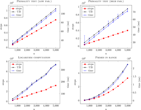
Figure 10: Execution steps vs. time (Intel^® Core^TM i7-4790 at 3.60GHz, 16 GB).

In the previous section we proved that the execution of compiled Haskell programs has the same resource consumption as the original ABS traces wrt. any concrete cost model $\mathcal{M}$, i.e., both programs execute the same ABS statements in the same order and in the same objects. However, cost models are defined in terms of ABS statements so they are unaware of low-level details of the Haskell runtime environment as $\beta$-reductions or garbage collection. Studying the relation between cost models and some significant low-level details of the Haskell runtime in a formal way is an interesting line of future work. In this section we address empirically one particular topic: the Haskell runtime does not introduce additional overhead, i.e., the execution of one ABS statement requires only a constant amount of work. In order to evaluate this hypothesis, we have elaborated programs with different asymptotic costs and measured the number of statements executed (steps) and their run-time. The Primality test computes the primality of a number $n$: the program creates $n$ objects and checks every possible divisor of $n$ on each object. The difference is that the low paralellism version awaits for the result of one divisor before invoking the next check and the high parallelism version does not. Both programs have a $O(n)$ cost. The Logarithm computation program computes the integer part $n$ logarithms. It has cost $O(n.\mathit{log}~{}n)$. Finally Primes in a range computes the prime numbers in the interval $[1..n]$, thus having a $O(n^{2})$ cost.

We have tested the programs with $n$ ranging from $500$ to $5000$, running $20$ experiments for every value of $n$, and measured the time. This is plotted in the cross line (right margin) in Fig. 10. The plot represents the mode times and the minimum and maximum times as whiskers. We have also measured the actual number of steps, represented in the square line (left margin) in Fig. 10. These two plots show that the execution time and the number of executed steps grows with a similar rate in all the programs, independently of their asymptotical cost, thus confirming that the compilation does not incur any overhead.

We have also plotted the resource bounds obtained by the SACO tool [2] for the different values of $n$ (triangle line, left margin in Fig. 10). SACO can analyze full ABS programs and thus also the subset considered in this paper, and allows the selection of the cost model of interest. In this case we have analyzed the original ABS programs using the cost model that obtains the number of ABS statements executed. As can be appreciated, the upper bounds are sound and overapproximate the actual number of executed statements. The difference between the upper bounds and the actual number of statements executed is explained for two reasons. First, the SACO tool considers constructor methods, i.e., methods that are invoked on every new object, so the SACO tool will count a constant number of extra statements whenever a new object is created. However, the main source of imprecision are branching points where SACO combines different fragments of information. A clear example are loops like the one in the Primes in a range program. The main loop checks if a number $i\in[1..n]$ is a prime number on each iteration, and this check needs the execution of $i$ statements. In this situation SACO considers that every iteration has the maximum cost ($n$ statements) and generate an upper bound of $n^{2}$ instead of the more precise (but asymptotically equivalent) expression $1+2+\ldots+n$.

6 Conclusion and Future Work

We have presented a concurrent object-oriented language (a subset of ABS) and its compilation to Haskell using continuations. The compilation is formalised in order to establish that the program behaviour and the resource consumption are preserved by the translation. Compared to the only other formalised ABS backend [9] (in Maude), our Haskell translation admits the preservation of resource consumption, and as a side benefit, makes uses of an overall faster backend.

In the future we plan to extend our formalisations to accommodate full ABS, both in terms of the omitted parts of the language as well as the non-deterministic behaviour of a multi-threaded scheduler, e.g. by broadening our simulated scheduler to non-determinism, and perhaps (M:N) thread parallelism. Another consideration is to relate our resource-preservation result to a distributed-object extension of ABS [4]; specifically, how the resource analysis translates to network transport costs after any network optimizations or protocol limitations. Finally, we plan to formally relate the ABS cost models used to define the cost of a trace and some of the low-level runtime details of the Haskell runtime like $\beta$-reductions, garbage collections or main memory usage. Thus, we could express trace costs and upper bounds in terms closer to the actual running environment.

References

- [1] Albert, E., Arenas, P., Correas, J., Genaim, S., Gómez-Zamalloa, M., Puebla, G., Román-Díez, G.: Object-Sensitive Cost Analysis for Concurrent Objects. Softw. Test. Verif. Reliab. 25(3), 218–271 (2015)
- [2] Albert, E., Arenas, P., Flores-Montoya, A., Genaim, S., Gómez-Zamalloa, M., Martin-Martin, E., Puebla, G., Román-Díez, G.: SACO: Static Analyzer for Concurrent Objects. In: Proc. TACAS ’14, pp. 562–567. LNCS 8413, Springer (2014)
- [3] Albert, E., Arenas, P., Gómez-Zamalloa, M.: Symbolic Execution of Concurrent Objects in CLP. In: Proc. PADL ’12. pp. 123–137. LNCS 7149, Springer (2012)
- [4] Bezirgiannis, N., de Boer, F.S.: ABS: A High-Level Modeling Language for Cloud-Aware Programming. In: Proc. SOFSEM ’16. Springer (2016), to appear
- [5] de Boer, F.S., Clarke, D., Johnsen, E.B.: A Complete Guide to the Future. In: Proc. ESOP ’07, pp. 316–330. LNCS 4421, Springer (2007)
- [6] Claessen, K., Hughes, J.: QuickCheck: A Lightweight Tool for Random Testing of Haskell Programs. In: Proc. ICFP ’00. pp. 268–279. ACM (2000)
- [7] Dean, J., Ghemawat, S.: MapReduce: Simplified Data Processing on Large Clusters. Commun. ACM 51(1), 107–113 (2008)
- [8] Flanagan, C., Felleisen, M.: The Semantics of Future and its Use in Program Optimization. In: Proc. POPL ’95. pp. 209–220. ACM (1995)
- [9] Johnsen, E.B., Hähnle, R., Schäfer, J., Schlatte, R., Steffen, M.: ABS: A Core Language for Abstract Behavioral Specification. In: FMCO ’10. pp. 142–164. LNCS 6957, Springer (2010)
- [10] Knuth, D.E.: The Art of Computer Programming, Volume 1: Fundamental Algorithms, 2nd Edition. Addison-Wesley Professional (1973)
- [11] Nakata, K., Saar, A.: Compiling Cooperative Task Management to Continuations. In: Proc. FSEN ’ 13, pp. 95–110. LNCS 8161, Springer (2013)
- [12] Nipkow, T., Wenzel, M., Paulson, L.C.: Isabelle/HOL: A Proof Assistant for Higher-order Logic. Springer-Verlag (2002)
- [13] Noll, T.: A Rewriting Logic Implementation of Erlang. ENTCS 44(2), 206–224 (2001), Proc. LDTA ’01
- [14] Palacios, A., Vidal, G.: Towards Modelling Actor-Based Concurrency in Term Rewriting. In: Proc. WPTE ’15. OASICS, vol. 46, pp. 19–29. Dagstuhl Pub. (2015)
- [15] Schäfer, J., Poetzsch-Heffter, A.: JCoBox: Generalizing Active Objects to Concurrent Components. In: ECOOP ’10, pp. 275–299. LNCS 6183, Springer (2010)
- [16] Srinivasan, S., Mycroft, A.: Kilim: Isolation-Typed Actors for Java. In: Proc. ECOOP ’08, pp. 104–128. LNCS 5142, Springer (2008)
- [17] Tarau, P.: Coordination and concurrency in multi-engine prolog. In: Proc. COORDINATION ’11. pp. 157–171. LNCS 6721, Springer (2011)
- [18] Vidal, G.: Towards Erlang Verification by Term Rewriting. In: Proc. LOPSTR ’13. pp. 109–126. LNCS 8901, Springer (2013)
- [19] Wong, P.Y., Albert, E., Muschevici, R., Proença, J., Schäfer, J., Schlatte, R.: The ABS Tool Suite: Modelling, Executing and Analysing Distributed Adaptable Object-Oriented Systems. STTT 14(5), 567–588 (2012)