Inverse Random Source Scattering for Elastic Waves

Gang Bao School of Mathematical Sciences, Zhejiang University, Hangzhou 310027, China; The research was supported in part by a Key Project of the Major Research Plan of NSFC (No. 91130004), an NSFC A3 Project (No.11421110002), NSFC Tianyuan Projects (No. 11426235; No. 11526211), and a special research grant from Zhejiang University. (baog@zju.edu.cn)    Chuchu Chen Department of Mathematics, Michigan State University, East Lansing, MI 48824, USA. (chen2095@math.purdue.edu)    Peijun Li Department of Mathematics, Purdue University, West Lafayette, Indiana 47907, USA. This author’s research was supported in part by the NSF grant DMS-1151308. (lipeijun@math.purdue.edu)
Abstract

This paper is concerned with the direct and inverse random source scattering problems for elastic waves where the source is assumed to be driven by an additive white noise. Given the source, the direct problem is to determine the displacement of the random wave field. The inverse problem is to reconstruct the mean and variance of the random source from the boundary measurement of the wave field at multiple frequencies. The direct problem is shown to have a unique mild solution by using a constructive proof. Based on the explicit mild solution, Fredholm integral equations of the first kind are deduced for the inverse problem. The regularized Kaczmarz method is presented to solve the ill-posed integral equations. Numerical experiments are included to demonstrate the effectiveness of the proposed method.

keywords:
Inverse source scattering problem, elastic wave equation, stochastic partial differential equation, Fredholm integral equation
AMS:
78A46, 65C30

1 Introduction

The inverse source scattering problems, an important research subject in inverse scattering theory, are to determine the unknown sources that generate prescribed radiated wave pattens [13, 23]. These problems are largely motivated by applications in medical imaging [19]. A typical example is to use electric or magnetic measurements on the surface of the human body, such as head, to infer the source currents inside the body, such as the brain, that produce the measured data. Mathematically, the inverse source scattering problems have been widely examined for acoustic and electromagnetic waves by many researchers [1, 2, 3, 8, 9, 32, 15, 17, 29]. For instance, it is known that the inverse source problem does not have a unique solution at a fixed frequency due to the existence of non-radiating sources [16, 21]; it is ill-posed as small variations in the measured data can lead to huge errors in the reconstructions [7].

Although the deterministic counterparts have been well studied, little is known for the stochastic inverse problems due to uncertainties, which are widely introduced to the models for two common reasons: randomness may directly appear in the studied systems [18, 20] and incomplete knowledge of the systems must be modeled by uncertainties [24]. A uniqueness result may be found in [14], where it showed that the auto-correlation function of the random source was uniquely determined everywhere outside the source region by the auto-correlation function of the radiated field. Recently, one-dimensional stochastic inverse source problems have been considered in [6, 10, 27], where the governing equations are stochastic ordinary differential equations. Utilizing the Green functions, the authors have presented the first approach in [5] for solving the inverse random source scattering problem in higher dimensions, where the stochastic partial differential equations are considered.

In this paper, we study both the direct and inverse random source scattering problems for elastic waves. Given the source, the direct problem is to determine the displacement of the random wave field. The inverse problem is to reconstruct the mean and variance of the random source from the boundary measurement of the wave field. Recently, the elastic wave scattering problems have received ever increasing attention for their significant applications in many scientific areas such as geophysics and seismology [11, 26, 28]. For example, they have played an important role in the problem for elastic pulse transmission and reflection through the Earth when investigating earthquakes and determining their focus, which is exactly the motivation of this work.

The random source is assumed to be driven by a white noise, which can be thought as the derivative of a Brownian sheet or a multi-parameter Brownian motion. The goal is to determine the mean and variance of the random source function by using the same statistics of the displacement of the wave field, which are measured on a boundary enclosing the compactly supported source at multiple frequencies. By constructing a sequence of regular processes approximating the rough white noise, we show that there exists a unique mild solution to the stochastic direct scattering problem. By studying the expectation and variance of the solution, we deduce Fredholm integral equations of the first kind for the inverse problem. It is known that Fredholm integral equations of the first kind are severely ill-posed, which can be clearly seen from the distribution of singular values for our integral equations. It is particularly true for the integral equations of reconstructing the variance. We present well conditioned integral equations via linear combination of the original equations. We propose a regularized Kaczmarz method to solve the resulting linear system of algebraic equations. This method is consistent with our multiple frequency data and requires solving a relatively small scale system at each iteration. Numerical experiments show that the proposed approach is effective to solve the problem.

This work is a nontrivial extension of the method proposed in [5] for the inverse random source scattering problem of the stochastic Helmholtz equation, to solve the inverse random source scattering problem of the stochastic Navier equation. Clearly, the elastic wave equation is more challenging due to the coexistence of compressional waves and shear waves that propagate at different speeds. The Green function is more complicated and has higher singularity for the Navier equation than that of the Helmholtz equation does. Hence more sophisticated analysis is required.

The paper is organized as follows. In section 2, we introduce the stochastic Navier equation for elastic waves and discuss the solutions of the deterministic and stochastic direct problems. Section 3 is devoted to the inverse problem, where Fredholm integral equations are deduced and the regularized Kaczmarz method is proposed to reconstruct the mean and the variance. Numerical experiments are presented in section 4 to illustrate the performance of the proposed method. The paper is concluded with general remarks in section 5.

2 Direct problem

In this section, we introduce the Navier equation for elastic waves and discuss the solutions of the deterministic and stochastic direct source scattering problems.

2.1 Problem formulation

Consider the scattering problem of the two-dimensional stochastic Navier equation in a homogeneous and isotropic medium

(1) μΔ𝒖+(λ+μ)𝒖+ω2𝒖=𝒇in2,𝜇Δ𝒖𝜆𝜇𝒖superscript𝜔2𝒖𝒇insuperscript2\mu\Delta\boldsymbol{u}+(\lambda+\mu)\nabla\nabla\cdot\boldsymbol{u}+\omega^{2}\boldsymbol{u}=\boldsymbol{f}\quad\text{in}~{}\mathbb{R}^{2},

where ω>0𝜔0\omega>0 is the angular frequency, λ𝜆\lambda and μ𝜇\mu are the Lamé constants satisfying μ>0𝜇0\mu>0 and λ+μ>0𝜆𝜇0\lambda+\mu>0, and 𝒖=(u1,u2)𝒖superscriptsubscript𝑢1subscript𝑢2top\boldsymbol{u}=(u_{1},u_{2})^{\top} is the displacement of the random wave field. As a source, the electric current density 𝒇=(f1,f2)𝒇superscriptsubscript𝑓1subscript𝑓2top\boldsymbol{f}=(f_{1},f_{2})^{\top} is assumed to be a random function driven by an additive white noise and takes the form

(2) 𝒇(x)=𝒈(x)+𝒉(x)W˙x.𝒇𝑥𝒈𝑥𝒉𝑥subscript˙𝑊𝑥\boldsymbol{f}(x)=\boldsymbol{g}(x)+\boldsymbol{h}(x)\dot{W}_{x}.

Here 𝒈=(g1,g2)𝒈superscriptsubscript𝑔1subscript𝑔2top\boldsymbol{g}=(g_{1},g_{2})^{\top} is a deterministic real vector function and 𝒉=diag(h1,h2)𝒉diagsubscript1subscript2\boldsymbol{h}={\rm diag}(h_{1},h_{2}) is a deterministic diagonal matrix function with hj0subscript𝑗0h_{j}\geq 0. We assume that gj,hj,j=1,2formulae-sequencesubscript𝑔𝑗subscript𝑗𝑗12g_{j},h_{j},j=1,2 have compact supports contained in the rectangular domain D2𝐷superscript2D\subset\mathbb{R}^{2}. W(x)=(W1(x),W2(x))𝑊𝑥superscriptsubscript𝑊1𝑥subscript𝑊2𝑥topW(x)=(W_{1}(x),W_{2}(x))^{\top} is a two-dimensional two-parameter Brownian sheet where W1(x)subscript𝑊1𝑥W_{1}(x) and W2(x)subscript𝑊2𝑥W_{2}(x) are two independent one-dimensional two-parameter Brownian sheets . W˙xsubscript˙𝑊𝑥\dot{W}_{x} is a white noise which can be thought as the derivative of the Brownian sheet Wxsubscript𝑊𝑥W_{x}. To make the paper self-contained, some preliminaries are presented in the appendix for the Brownian sheet, white noise, and corresponding stochastic integrals.

In this random source model, 𝒈𝒈\boldsymbol{g} and 𝒉𝒉\boldsymbol{h} can be viewed as the mean and standard deviation of 𝒇𝒇\boldsymbol{f}, respectively. Hence 𝒉2=diag(h12,h22)superscript𝒉2diagsuperscriptsubscript12superscriptsubscript22\boldsymbol{h}^{2}={\rm diag}(h_{1}^{2},h_{2}^{2}) is the variance of 𝒇𝒇\boldsymbol{f}. To ensure the uniqueness of the solution, the following Kupradze-Sommerfeld radiation condition is required for the radiated wave field:

(3) limrr1/2(r𝒖piκp𝒖p)=0,limrr1/2(r𝒖siκs𝒖s)=0,r=|x|,formulae-sequencesubscript𝑟superscript𝑟12subscript𝑟subscript𝒖pisubscript𝜅psubscript𝒖p0formulae-sequencesubscript𝑟superscript𝑟12subscript𝑟subscript𝒖sisubscript𝜅ssubscript𝒖s0𝑟𝑥\lim_{r\to\infty}r^{1/2}(\partial_{r}\boldsymbol{u}_{\rm p}-{\rm i}\kappa_{\rm p}\boldsymbol{u}_{\rm p})=0,\quad\lim_{r\to\infty}r^{1/2}(\partial_{r}\boldsymbol{u}_{\rm s}-{\rm i}\kappa_{\rm s}\boldsymbol{u}_{\rm s})=0,\quad r=|x|,

uniformly in all directions x^=x/|x|^𝑥𝑥𝑥\hat{x}=x/|x|, where

𝒖p=1κp2𝒖,𝒖s=1κs2×(×𝒖)formulae-sequencesubscript𝒖p1subscriptsuperscript𝜅2p𝒖subscript𝒖s1subscriptsuperscript𝜅2s𝒖\boldsymbol{u}_{\rm p}=-\frac{1}{\kappa^{2}_{\rm p}}\nabla\nabla\cdot\boldsymbol{u},\quad\boldsymbol{u}_{\rm s}=\frac{1}{\kappa^{2}_{\rm s}}\nabla\times(\nabla\times\boldsymbol{u})

are the compressional component and the shear component of 𝒖𝒖\boldsymbol{u}, respectively, and

κp=ωλ+2μ,κs=ωμformulae-sequencesubscript𝜅p𝜔𝜆2𝜇subscript𝜅s𝜔𝜇\kappa_{\rm p}=\frac{\omega}{\sqrt{\lambda+2\mu}},\quad\kappa_{\rm s}=\frac{\omega}{\sqrt{\mu}}

are known as the compressional wavenumber and the shear wavenumber, respectively.

Let BR={xd:|x|<R}subscript𝐵𝑅conditional-set𝑥superscript𝑑𝑥𝑅B_{R}=\{x\in\mathbb{R}^{d}:|x|<R\} be the ball with radius R𝑅R. Denote by BRsubscript𝐵𝑅\partial B_{R} the boundary of BRsubscript𝐵𝑅B_{R}. Let R𝑅R be large enough such that D¯BR¯𝐷subscript𝐵𝑅\bar{D}\subset B_{R}. Given the random electric current density function 𝒇𝒇\boldsymbol{f}, i.e., given 𝒈𝒈\boldsymbol{g} and 𝒉𝒉\boldsymbol{h}, the direct problem is to determine the random wave field 𝒖𝒖\boldsymbol{u} of the stochastic scattering problem (1) and (3). The inverse problem is to determine the mean 𝒈𝒈\boldsymbol{g} and the standard deviation 𝒉𝒉\boldsymbol{h} or the variance 𝒉2superscript𝒉2\boldsymbol{h}^{2} of the random source function from the measured random wave field on BRsubscript𝐵𝑅\partial B_{R} at a finite number of frequencies ωk,k=1,,Kformulae-sequencesubscript𝜔𝑘𝑘1𝐾\omega_{k},k=1,\dots,K.

2.2 Deterministic direct problem

We begin with the solution for the deterministic direct source problem. Let 𝒉=0𝒉0\boldsymbol{h}=0 in (2), i.e., no randomness is present in the source. The stochastic scattering problem reduces to the deterministic scattering problem:

(4) {μΔ𝒖+(λ+μ)𝒖+ω2𝒖=𝒈in2,r𝒖piκp𝒖p=o(r1/2)asr,r𝒖siκs𝒖s=o(r1/2)asr.cases𝜇Δ𝒖𝜆𝜇𝒖superscript𝜔2𝒖𝒈insuperscript2subscript𝑟subscript𝒖pisubscript𝜅psubscript𝒖p𝑜superscript𝑟12as𝑟subscript𝑟subscript𝒖sisubscript𝜅ssubscript𝒖s𝑜superscript𝑟12as𝑟\begin{cases}\mu\Delta\boldsymbol{u}+(\lambda+\mu)\nabla\nabla\cdot\boldsymbol{u}+\omega^{2}\boldsymbol{u}=\boldsymbol{g}\quad&\text{in}~{}\mathbb{R}^{2},\\[2.0pt] \partial_{r}\boldsymbol{u}_{\rm p}-{\rm i}\kappa_{\rm p}\boldsymbol{u}_{\rm p}=o(r^{-1/2})\quad&\text{as}~{}r\to\infty,\\[2.0pt] \partial_{r}\boldsymbol{u}_{\rm s}-{\rm i}\kappa_{\rm s}\boldsymbol{u}_{\rm s}=o(r^{-1/2})\quad&\text{as}~{}r\to\infty.\end{cases}

Given 𝒈L2(D)2𝒈superscript𝐿2superscript𝐷2\boldsymbol{g}\in L^{2}(D)^{2}, it is known that the scattering problem (4) has a unique solution

(5) 𝒖(x,ω)=D𝔾(x,y,ω)𝒈(y)dy,𝒖𝑥𝜔subscript𝐷𝔾𝑥𝑦𝜔𝒈𝑦differential-d𝑦\boldsymbol{u}(x,\omega)=\int_{D}\mathbb{G}(x,y,\omega)\boldsymbol{g}(y){\rm d}y,

where 𝔾𝔾\mathbb{G} is the Green tensor function of the Navier equation:

𝔾(x,y,ω)=i4μH0(1)(κs|xy|)𝕀+i4ω2xx[H0(1)(κs|xy|)H0(1)(κp|xy|)].𝔾𝑥𝑦𝜔i4𝜇superscriptsubscript𝐻01subscript𝜅s𝑥𝑦𝕀i4superscript𝜔2subscript𝑥superscriptsubscript𝑥topsuperscriptsubscript𝐻01subscript𝜅s𝑥𝑦superscriptsubscript𝐻01subscript𝜅p𝑥𝑦\displaystyle\mathbb{G}(x,y,\omega)=\frac{\rm i}{4\mu}H_{0}^{(1)}(\kappa_{\rm s}|x-y|)\mathbb{I}+\frac{\rm i}{4\omega^{2}}\nabla_{x}\nabla_{x}^{\top}\Bigl{[}H_{0}^{(1)}(\kappa_{\rm s}|x-y|)-H_{0}^{(1)}(\kappa_{\rm p}|x-y|)\Bigr{]}.

Here 𝕀𝕀\mathbb{I} is the 2×2222\times 2 identity matrix, H0(1)superscriptsubscript𝐻01H_{0}^{(1)} is the Hankel function of the first kind with order zero, and

xx=(x1x1x1x2x1x2x2x2).subscript𝑥superscriptsubscript𝑥topmatrixsubscriptsubscript𝑥1subscript𝑥1subscriptsubscript𝑥1subscript𝑥2subscriptsubscript𝑥1subscript𝑥2subscriptsubscript𝑥2subscript𝑥2\nabla_{x}\nabla_{x}^{\top}=\begin{pmatrix}\partial_{x_{1}x_{1}}&\partial_{x_{1}x_{2}}\\ \partial_{x_{1}x_{2}}&\partial_{x_{2}x_{2}}\end{pmatrix}.

It is known that this Green tensor function has an equivalent form

(6) 𝔾(x,y,ω)=G1(|xy|)𝕀+G2(|xy|)𝕁(xy),𝔾𝑥𝑦𝜔subscript𝐺1𝑥𝑦𝕀subscript𝐺2𝑥𝑦𝕁𝑥𝑦\mathbb{G}(x,y,\omega)=G_{1}(|x-y|)\mathbb{I}+G_{2}(|x-y|)\mathbb{J}(x-y),

which plays an vital role in derivation of the subsequent regularity analysis. Here for x2\{0}𝑥\superscript20x\in{\mathbb{R}}^{2}\backslash\{0\}, the matrix 𝕁𝕁\mathbb{J} is given by

𝕁(x)=xx|x|2.𝕁𝑥𝑥superscript𝑥topsuperscript𝑥2\mathbb{J}(x)=\frac{xx^{\top}}{|x|^{2}}.

It is shown in [25] that the functions G1subscript𝐺1G_{1} and G2subscript𝐺2G_{2} can be decomposed into

(7) Gj(v)=1πlog(v)Φj(v)+ηj(v),j=1,2,formulae-sequencesubscript𝐺𝑗𝑣1𝜋𝑣subscriptΦ𝑗𝑣subscript𝜂𝑗𝑣𝑗12G_{j}(v)=\frac{1}{\pi}\log(v)\Phi_{j}(v)+\eta_{j}(v),\quad j=1,2,

where ΦjsubscriptΦ𝑗\Phi_{j} and ηjsubscript𝜂𝑗\eta_{j} are analytic functions. Explicitly, we have

(8) Φ1(v)=α+β1v2+O(v4),Φ2=β2v2+O(v4)formulae-sequencesubscriptΦ1𝑣𝛼subscript𝛽1superscript𝑣2𝑂superscript𝑣4subscriptΦ2subscript𝛽2superscript𝑣2𝑂superscript𝑣4\Phi_{1}(v)=\alpha+\beta_{1}v^{2}+O(v^{4}),\quad\Phi_{2}=\beta_{2}v^{2}+O(v^{4})

and

(9) η1(v)=γ1+O(v2),η2=γ2+O(v2)formulae-sequencesubscript𝜂1𝑣subscript𝛾1𝑂superscript𝑣2subscript𝜂2subscript𝛾2𝑂superscript𝑣2\eta_{1}(v)=\gamma_{1}+O(v^{2}),\quad\eta_{2}=\gamma_{2}+O(v^{2})

for v0𝑣0v\rightarrow 0, where α𝛼\alpha, βjsubscript𝛽𝑗\beta_{j}, and γjsubscript𝛾𝑗\gamma_{j} are constants depending on ω𝜔\omega, μ𝜇\mu, and λ𝜆\lambda.

The following regularity results of the Green tensor function play an important role in the analysis of the stochastic direct scattering problem.

Lemma 1.

Let Ω2Ωsuperscript2\Omega\subset\mathbb{R}^{2} be a bounded domain. Then 𝔾(,y)L2(Ω),yΩformulae-sequencenorm𝔾𝑦superscript𝐿2Ωfor-all𝑦Ω\|\mathbb{G}(\cdot,y)\|\in L^{2}(\Omega),\,\forall\,y\in\Omega, i.e.

Ω𝔾(x,y,ω)2dx<,subscriptΩsuperscriptnorm𝔾𝑥𝑦𝜔2differential-d𝑥\int_{\Omega}\|\mathbb{G}(x,y,\omega)\|^{2}{\rm d}x<\infty,

where \|\cdot\| is the Frobenius norm.

Proof.

Let a=supx,yΩ|xy|𝑎subscriptsupremum𝑥𝑦Ω𝑥𝑦a=\sup_{x,y\in\Omega}|x-y|. We have Ω¯Ba(y)¯Ωsubscript𝐵𝑎𝑦\bar{\Omega}\subset B_{a}(y), where Ba(y)subscript𝐵𝑎𝑦B_{a}(y) is the ball with radius a𝑎a and center at y𝑦y. Since J(w)=1norm𝐽𝑤1\|J(w)\|=1, it follows from the expression in (6) and (7) that we only need to show that

log(|xy|)|xy|mL2(Ω),yΩ,m0.formulae-sequence𝑥𝑦superscript𝑥𝑦𝑚superscript𝐿2Ωformulae-sequencefor-all𝑦Ω𝑚0\log(|x-y|)|x-y|^{m}\in L^{2}(\Omega),\quad\forall\,y\in\Omega,~{}m\geq 0.

A simple calculation yields

Ω|log(|xy|)|xy|m|2dxsubscriptΩsuperscript𝑥𝑦superscript𝑥𝑦𝑚2differential-d𝑥\displaystyle\int_{\Omega}\Bigl{|}\log(|x-y|)|x-y|^{m}\Bigr{|}^{2}{\rm d}x Ba(y)|log(|xy|)|xy|m|2dxabsentsubscriptsubscript𝐵𝑎𝑦superscript𝑥𝑦superscript𝑥𝑦𝑚2differential-d𝑥\displaystyle\leq\int_{B_{a}(y)}\Bigl{|}\log(|x-y|)|x-y|^{m}\Bigr{|}^{2}{\rm d}x
0ar1+2m|log(r)|2dr<,less-than-or-similar-toabsentsuperscriptsubscript0𝑎superscript𝑟12𝑚superscript𝑟2differential-d𝑟\displaystyle\lesssim\int_{0}^{a}r^{1+2m}\Bigl{|}\log(r)\Bigr{|}^{2}{\rm d}r<\infty,

which completes the proof. ∎

Throughout the paper, abless-than-or-similar-to𝑎𝑏a\lesssim b stands for aCb𝑎𝐶𝑏a\leq Cb, where C𝐶C is a positive constant and its specific value is not required but should be clear from the context.

Lemma 2.

Let Ω2Ωsuperscript2\Omega\subset\mathbb{R}^{2} be a bounded domain. We have for α(32,)𝛼32\alpha\in(\frac{3}{2},\,\infty) that

(10) Ω𝔾(x,y,ω)𝔾(x,z,ω)αdx|yz|32,y,zΩ.formulae-sequenceless-than-or-similar-tosubscriptΩsuperscriptnorm𝔾𝑥𝑦𝜔𝔾𝑥𝑧𝜔𝛼differential-d𝑥superscript𝑦𝑧32for-all𝑦𝑧Ω\int_{\Omega}\|\mathbb{G}(x,y,\omega)-\mathbb{G}(x,z,\omega)\|^{\alpha}{\rm d}x\lesssim|y-z|^{\frac{3}{2}},\quad\forall~{}y,z\in\Omega.
Proof.

It follows from (6) and the triangle inequality that

Ω𝔾(x,y,ω)𝔾(x,z,ω)αdxsubscriptΩsuperscriptnorm𝔾𝑥𝑦𝜔𝔾𝑥𝑧𝜔𝛼differential-d𝑥\displaystyle\int_{\Omega}\|\mathbb{G}(x,y,\omega)-\mathbb{G}(x,z,\omega)\|^{\alpha}{\rm d}x
ΩG1(|xy|)𝕀G1(|xz|)𝕀αdxless-than-or-similar-toabsentsubscriptΩsuperscriptdelimited-∥∥subscript𝐺1𝑥𝑦𝕀subscript𝐺1𝑥𝑧𝕀𝛼differential-d𝑥\displaystyle\lesssim\int_{\Omega}\Bigl{\|}G_{1}(|x-y|)\mathbb{I}-G_{1}(|x-z|)\mathbb{I}\Bigr{\|}^{\alpha}{\rm d}x
+ΩG2(|xy|)𝕁(xy)G2(|xz|)𝕁(xz)αdxsubscriptΩsuperscriptdelimited-∥∥subscript𝐺2𝑥𝑦𝕁𝑥𝑦subscript𝐺2𝑥𝑧𝕁𝑥𝑧𝛼differential-d𝑥\displaystyle\hskip 113.81102pt+\int_{\Omega}\Bigl{\|}G_{2}(|x-y|)\mathbb{J}(x-y)-G_{2}(|x-z|)\mathbb{J}(x-z)\Bigr{\|}^{\alpha}{\rm d}x
Ω|G1(|xy|)G1(|xz|)|αdx+Ω|G2(|xy|)G2(|xz|)|α𝕁(xy)αdxless-than-or-similar-toabsentsubscriptΩsuperscriptsubscript𝐺1𝑥𝑦subscript𝐺1𝑥𝑧𝛼differential-d𝑥subscriptΩsuperscriptsubscript𝐺2𝑥𝑦subscript𝐺2𝑥𝑧𝛼superscriptnorm𝕁𝑥𝑦𝛼differential-d𝑥\displaystyle\lesssim\int_{\Omega}\Bigl{|}G_{1}(|x-y|)-G_{1}(|x-z|)\Bigr{|}^{\alpha}{\rm d}x+\int_{\Omega}\Bigl{|}G_{2}(|x-y|)-G_{2}(|x-z|)\Bigr{|}^{\alpha}\|\mathbb{J}(x-y)\|^{\alpha}{\rm d}x
+Ω|G2(|xz|)|α𝕁(xy)𝕁(xz)αdxsubscriptΩsuperscriptsubscript𝐺2𝑥𝑧𝛼superscriptnorm𝕁𝑥𝑦𝕁𝑥𝑧𝛼differential-d𝑥\displaystyle\hskip 113.81102pt+\int_{\Omega}|G_{2}(|x-z|)|^{\alpha}\|\mathbb{J}(x-y)-\mathbb{J}(x-z)\|^{\alpha}{\rm d}x
=:T1+T2+T3.\displaystyle=:T_{1}+T_{2}+T_{3}.

We shall only present the estimates of T1subscript𝑇1T_{1} and T3subscript𝑇3T_{3} since the estimates of T1subscript𝑇1T_{1} and T2subscript𝑇2T_{2} are similar due to 𝕁(x)=1norm𝕁𝑥1\|\mathbb{J}(x)\|=1 and (7).

Step 1. The estimate of T1subscript𝑇1T_{1}. It suffices to estimate the singular part G1subscript𝐺1G_{1} of T1subscript𝑇1T_{1}. It follows from (7), (8), and (9) that we have

T1less-than-or-similar-tosubscript𝑇1absent\displaystyle T_{1}\lesssim Ω|log(|xy|)log(|xz|)|αdx+Ω||xy|p|xz|p|αdxsubscriptΩsuperscript𝑥𝑦𝑥𝑧𝛼differential-d𝑥subscriptΩsuperscriptsuperscript𝑥𝑦𝑝superscript𝑥𝑧𝑝𝛼differential-d𝑥\displaystyle\int_{\Omega}\Bigl{|}\log(|x-y|)-\log(|x-z|)\Bigr{|}^{\alpha}{\rm d}x+\int_{\Omega}\Bigl{|}|x-y|^{p}-|x-z|^{p}\Bigr{|}^{\alpha}{\rm d}x
+Ω|log(|xy|)|xy|plog(|xz|)|xz|p|αdxsubscriptΩsuperscript𝑥𝑦superscript𝑥𝑦𝑝𝑥𝑧superscript𝑥𝑧𝑝𝛼differential-d𝑥\displaystyle+\int_{\Omega}\Bigl{|}\log(|x-y|)|x-y|^{p}-\log(|x-z|)|x-z|^{p}\Bigr{|}^{\alpha}{\rm d}x
=:absent:\displaystyle=: T11+T12+T13,superscriptsubscript𝑇11superscriptsubscript𝑇12superscriptsubscript𝑇13\displaystyle T_{1}^{1}+T_{1}^{2}+T_{1}^{3},

where p=2𝑝2p=2 or 444.

For the term T11superscriptsubscript𝑇11T_{1}^{1}, we have

T11=superscriptsubscript𝑇11absent\displaystyle T_{1}^{1}= Ω||xy||xz||32|log(|xy|)log(|xz|)|α32subscriptΩsuperscript𝑥𝑦𝑥𝑧32superscript𝑥𝑦𝑥𝑧𝛼32\displaystyle\int_{\Omega}\Bigl{|}|x-y|-|x-z|\Bigr{|}^{\frac{3}{2}}\Bigl{|}\log(|x-y|)-\log(|x-z|)\Bigr{|}^{\alpha-\frac{3}{2}}
×|01(|xy|t+|xz|(1t))1dt|32dxabsentsuperscriptsuperscriptsubscript01superscript𝑥𝑦𝑡𝑥𝑧1𝑡1differential-d𝑡32d𝑥\displaystyle\hskip 113.81102pt\times\left|\int_{0}^{1}\Bigl{(}|x-y|t+|x-z|(1-t)\Bigr{)}^{-1}{\rm d}t\right|^{\frac{3}{2}}{\rm d}x
\displaystyle\leq |yz|32Ω|log(|xy|)log(|xz|)|α32|1|xy|+1|xz||32dxsuperscript𝑦𝑧32subscriptΩsuperscript𝑥𝑦𝑥𝑧𝛼32superscript1𝑥𝑦1𝑥𝑧32differential-d𝑥\displaystyle|y-z|^{\frac{3}{2}}\int_{\Omega}\Bigl{|}\log(|x-y|)-\log(|x-z|)\Bigr{|}^{\alpha-\frac{3}{2}}\left|\frac{1}{|x-y|}+\frac{1}{|x-z|}\right|^{\frac{3}{2}}{\rm d}x
\displaystyle\leq |yz|32(Ω(1|xy|+1|xz|)95dx)56superscript𝑦𝑧32superscriptsubscriptΩsuperscript1𝑥𝑦1𝑥𝑧95differential-d𝑥56\displaystyle|y-z|^{\frac{3}{2}}\left(\int_{\Omega}\Bigl{(}\frac{1}{|x-y|}+\frac{1}{|x-z|}\Bigr{)}^{\frac{9}{5}}{\rm d}x\right)^{\frac{5}{6}}
×(Ω|log(|xy|)log(|xz|)|6α9dx)16,absentsuperscriptsubscriptΩsuperscript𝑥𝑦𝑥𝑧6𝛼9differential-d𝑥16\displaystyle\hskip 113.81102pt\times\left(\int_{\Omega}\Bigl{|}\log(|x-y|)-\log(|x-z|)\Bigr{|}^{6\alpha-9}{\rm d}x\right)^{\frac{1}{6}},

where we have used the Hölder inequality in the last step.

Let a=supx,yΩ|xy|𝑎subscriptsupremum𝑥𝑦Ω𝑥𝑦a=\sup_{x,y\in\Omega}|x-y| and b=supx,zΩ|xz|𝑏subscriptsupremum𝑥𝑧Ω𝑥𝑧b=\sup_{x,z\in\Omega}|x-z|. We have Ω¯Ba(y)¯Ωsubscript𝐵𝑎𝑦\bar{\Omega}\subset B_{a}(y) and Ω¯Bb(z)¯Ωsubscript𝐵𝑏𝑧\bar{\Omega}\subset B_{b}(z), where Ba(y)subscript𝐵𝑎𝑦B_{a}(y) and Bb(z)subscript𝐵𝑏𝑧B_{b}(z) are the discs with radii a𝑎a and b𝑏b and centers at y𝑦y and z𝑧z, respectively. It is easy to verify that

Ω(1|xy|+1|xz|)95dxsubscriptΩsuperscript1𝑥𝑦1𝑥𝑧95differential-d𝑥\displaystyle\int_{\Omega}\Bigl{(}\frac{1}{|x-y|}+\frac{1}{|x-z|}\Bigr{)}^{\frac{9}{5}}{\rm d}x Ba(y)1|xy|95dx+Bb(z)1|xz|95dxless-than-or-similar-toabsentsubscriptsubscript𝐵𝑎𝑦1superscript𝑥𝑦95differential-d𝑥subscriptsubscript𝐵𝑏𝑧1superscript𝑥𝑧95differential-d𝑥\displaystyle\lesssim\int_{B_{a}(y)}\frac{1}{|x-y|^{\frac{9}{5}}}{\rm d}x+\int_{B_{b}(z)}\frac{1}{|x-z|^{\frac{9}{5}}}{\rm d}x
0ar45dr+0br45dr<less-than-or-similar-toabsentsuperscriptsubscript0𝑎superscript𝑟45differential-d𝑟superscriptsubscript0𝑏superscript𝑟45differential-d𝑟\displaystyle\lesssim\int_{0}^{a}r^{-\frac{4}{5}}{\rm d}r+\int_{0}^{b}r^{-\frac{4}{5}}{\rm d}r<\infty

and

Ω|log(|xy|)log(|xz|)|6α9dxsubscriptΩsuperscript𝑥𝑦𝑥𝑧6𝛼9differential-d𝑥\displaystyle\int_{\Omega}\Bigl{|}\log(|x-y|)-\log(|x-z|)\Bigr{|}^{6\alpha-9}{\rm d}x
Ba(y)|log(|xy|)|6α9dx+Bb(z)|log(|xz|)|6α9dxless-than-or-similar-toabsentsubscriptsubscript𝐵𝑎𝑦superscript𝑥𝑦6𝛼9differential-d𝑥subscriptsubscript𝐵𝑏𝑧superscript𝑥𝑧6𝛼9differential-d𝑥\displaystyle\lesssim\int_{B_{a}(y)}\Bigl{|}\log(|x-y|)\Bigr{|}^{6\alpha-9}{\rm d}x+\int_{B_{b}(z)}\Bigl{|}\log(|x-z|)\Bigr{|}^{6\alpha-9}{\rm d}x
0ar|log(r)|6α9dr+0br|log(r)|6α9dr<.less-than-or-similar-toabsentsuperscriptsubscript0𝑎𝑟superscript𝑟6𝛼9differential-d𝑟superscriptsubscript0𝑏𝑟superscript𝑟6𝛼9differential-d𝑟\displaystyle\lesssim\int_{0}^{a}r\Bigl{|}\log(r)\Bigr{|}^{6\alpha-9}{\rm d}r+\int_{0}^{b}r\Bigl{|}\log(r)\Bigr{|}^{6\alpha-9}{\rm d}r<\infty.

Combining the above estimates gives T11|yz|32less-than-or-similar-tosuperscriptsubscript𝑇11superscript𝑦𝑧32T_{1}^{1}\lesssim|y-z|^{\frac{3}{2}}.

For the term T12superscriptsubscript𝑇12T_{1}^{2}, using the identity

apbp=(ab)(ap1+ap2b++abp2+bp1),superscript𝑎𝑝superscript𝑏𝑝𝑎𝑏superscript𝑎𝑝1superscript𝑎𝑝2𝑏𝑎superscript𝑏𝑝2superscript𝑏𝑝1a^{p}-b^{p}=(a-b)\bigl{(}a^{p-1}+a^{p-2}b+\cdots+ab^{p-2}+b^{p-1}\bigr{)},

we obtain

T12superscriptsubscript𝑇12\displaystyle T_{1}^{2} |yz|αΩ[|xy|(p1)α+|xy|(p2)α|xz|α++|xz|(p1)α]dxless-than-or-similar-toabsentsuperscript𝑦𝑧𝛼subscriptΩdelimited-[]superscript𝑥𝑦𝑝1𝛼superscript𝑥𝑦𝑝2𝛼superscript𝑥𝑧𝛼superscript𝑥𝑧𝑝1𝛼differential-d𝑥\displaystyle\lesssim|y-z|^{\alpha}\int_{\Omega}\Bigl{[}|x-y|^{(p-1)\alpha}+|x-y|^{(p-2)\alpha}|x-z|^{\alpha}+\cdots+|x-z|^{(p-1)\alpha}\Bigr{]}{\rm d}x
|yz|α.less-than-or-similar-toabsentsuperscript𝑦𝑧𝛼\displaystyle\lesssim|y-z|^{\alpha}.

Applying the technique of estimating the terms T11superscriptsubscript𝑇11T_{1}^{1} and T12superscriptsubscript𝑇12T_{1}^{2}, we get the estimate for the term T13superscriptsubscript𝑇13T_{1}^{3}:

T13superscriptsubscript𝑇13\displaystyle T_{1}^{3} Ω|log(|xy|)|α||xy|p|xz|p|αdxless-than-or-similar-toabsentsubscriptΩsuperscript𝑥𝑦𝛼superscriptsuperscript𝑥𝑦𝑝superscript𝑥𝑧𝑝𝛼differential-d𝑥\displaystyle\lesssim\int_{\Omega}\Bigl{|}\log(|x-y|)\Bigr{|}^{\alpha}\Bigl{|}|x-y|^{p}-|x-z|^{p}\Bigr{|}^{\alpha}{\rm d}x
+Ω|log(|xy|)log(|xz|)|α|xz|pαdxsubscriptΩsuperscript𝑥𝑦𝑥𝑧𝛼superscript𝑥𝑧𝑝𝛼differential-d𝑥\displaystyle\hskip 113.81102pt+\int_{\Omega}\Bigl{|}\log(|x-y|)-\log(|x-z|)\Bigr{|}^{\alpha}|x-z|^{p\alpha}{\rm d}x
|yz|αΩ|log(|xy|)|α[|xy|(p1)α+|xy|(p2)α|xz|α++|xz|(p1)α]dxless-than-or-similar-toabsentsuperscript𝑦𝑧𝛼subscriptΩsuperscript𝑥𝑦𝛼delimited-[]superscript𝑥𝑦𝑝1𝛼superscript𝑥𝑦𝑝2𝛼superscript𝑥𝑧𝛼superscript𝑥𝑧𝑝1𝛼differential-d𝑥\displaystyle\lesssim|y-z|^{\alpha}\int_{\Omega}\Bigl{|}\log(|x-y|)\Bigr{|}^{\alpha}\Bigl{[}|x-y|^{(p-1)\alpha}+|x-y|^{(p-2)\alpha}|x-z|^{\alpha}+\cdots+|x-z|^{(p-1)\alpha}\Bigr{]}{\rm d}x
+|yz|32Ω|log(|xy|)log(|xz|)|α32|1|xy|+1|xz||32|xz|pαdxsuperscript𝑦𝑧32subscriptΩsuperscript𝑥𝑦𝑥𝑧𝛼32superscript1𝑥𝑦1𝑥𝑧32superscript𝑥𝑧𝑝𝛼differential-d𝑥\displaystyle\quad+|y-z|^{\frac{3}{2}}\int_{\Omega}\Bigl{|}\log(|x-y|)-\log(|x-z|)\Bigr{|}^{\alpha-\frac{3}{2}}\left|\frac{1}{|x-y|}+\frac{1}{|x-z|}\right|^{\frac{3}{2}}|x-z|^{p\alpha}{\rm d}x
|yz|α+|yz|32.less-than-or-similar-toabsentsuperscript𝑦𝑧𝛼superscript𝑦𝑧32\displaystyle\lesssim|y-z|^{\alpha}+|y-z|^{\frac{3}{2}}.

Therefore, we obtain T1|yz|32subscript𝑇1superscript𝑦𝑧32T_{1}\leq|y-z|^{\frac{3}{2}} for α>32𝛼32\alpha>\frac{3}{2}. Similarly, we may have the estimate T2|yz|32subscript𝑇2superscript𝑦𝑧32T_{2}\leq|y-z|^{\frac{3}{2}}.

Step 2. The estimate of term T3subscript𝑇3T_{3}. Recall

𝕁(x)=[J11(x)J12(x)J12(x)J22(x)]=[x12|x|2x1x2|x|2x1x2|x|2x22|x|2].𝕁𝑥matrixsubscript𝐽11𝑥subscript𝐽12𝑥subscript𝐽12𝑥subscript𝐽22𝑥matrixsuperscriptsubscript𝑥12superscript𝑥2subscript𝑥1subscript𝑥2superscript𝑥2subscript𝑥1subscript𝑥2superscript𝑥2superscriptsubscript𝑥22superscript𝑥2\mathbb{J}(x)=\begin{bmatrix}J_{11}(x)&J_{12}(x)\\ J_{12}(x)&J_{22}(x)\end{bmatrix}=\begin{bmatrix}\frac{x_{1}^{2}}{|x|^{2}}&\frac{x_{1}x_{2}}{|x|^{2}}\\ \frac{x_{1}x_{2}}{|x|^{2}}&\frac{x_{2}^{2}}{|x|^{2}}\end{bmatrix}.

A simple calculation yields

𝕁(xy)𝕁(xz)2superscriptnorm𝕁𝑥𝑦𝕁𝑥𝑧2\displaystyle\|\mathbb{J}(x-y)-\mathbb{J}(x-z)\|^{2} =|J11(xy)J11(xz)|2absentsuperscriptsubscript𝐽11𝑥𝑦subscript𝐽11𝑥𝑧2\displaystyle=|J_{11}(x-y)-J_{11}(x-z)|^{2}
+2|J12(xy)J12(xz)|2+|J22(xy)J22(xz)|2.2superscriptsubscript𝐽12𝑥𝑦subscript𝐽12𝑥𝑧2superscriptsubscript𝐽22𝑥𝑦subscript𝐽22𝑥𝑧2\displaystyle+2|J_{12}(x-y)-J_{12}(x-z)|^{2}+|J_{22}(x-y)-J_{22}(x-z)|^{2}.

It is easy to verify that

|J11(xy)J11(xz)|subscript𝐽11𝑥𝑦subscript𝐽11𝑥𝑧\displaystyle|J_{11}(x-y)-J_{11}(x-z)|
=\displaystyle= |(x1y1)2|xy|2(x1z1)2|xz|2|superscriptsubscript𝑥1subscript𝑦12superscript𝑥𝑦2superscriptsubscript𝑥1subscript𝑧12superscript𝑥𝑧2\displaystyle\left|\frac{(x_{1}-y_{1})^{2}}{|x-y|^{2}}-\frac{(x_{1}-z_{1})^{2}}{|x-z|^{2}}\right|
=\displaystyle= |(x1y1|xy|+x1z1|xz|)(x1y1|xy|x1z1|xz|)|subscript𝑥1subscript𝑦1𝑥𝑦subscript𝑥1subscript𝑧1𝑥𝑧subscript𝑥1subscript𝑦1𝑥𝑦subscript𝑥1subscript𝑧1𝑥𝑧\displaystyle\left|\Big{(}\frac{x_{1}-y_{1}}{|x-y|}+\frac{x_{1}-z_{1}}{|x-z|}\Big{)}\Big{(}\frac{x_{1}-y_{1}}{|x-y|}-\frac{x_{1}-z_{1}}{|x-z|}\Big{)}\right|
less-than-or-similar-to\displaystyle\lesssim |x1y1|xy|x1z1|xz||subscript𝑥1subscript𝑦1𝑥𝑦subscript𝑥1subscript𝑧1𝑥𝑧\displaystyle\left|\frac{x_{1}-y_{1}}{|x-y|}-\frac{x_{1}-z_{1}}{|x-z|}\right|
=\displaystyle= |(|xz||xy|)(x1y1)+|xy|((x1y1)(x1z1))|xy||xz||𝑥𝑧𝑥𝑦subscript𝑥1subscript𝑦1𝑥𝑦subscript𝑥1subscript𝑦1subscript𝑥1subscript𝑧1𝑥𝑦𝑥𝑧\displaystyle\left|\frac{\big{(}|x-z|-|x-y|\big{)}(x_{1}-y_{1})+|x-y|\big{(}(x_{1}-y_{1})-(x_{1}-z_{1})\big{)}}{|x-y||x-z|}\right|
less-than-or-similar-to\displaystyle\lesssim |yz||xz|.𝑦𝑧𝑥𝑧\displaystyle\frac{|y-z|}{|x-z|}.

Similarly, we may show that

|J22(xy)J22(xz)|=|(x2y2)2|xy|2(x2z2)2|xz|2||yz||xz|subscript𝐽22𝑥𝑦subscript𝐽22𝑥𝑧superscriptsubscript𝑥2subscript𝑦22superscript𝑥𝑦2superscriptsubscript𝑥2subscript𝑧22superscript𝑥𝑧2less-than-or-similar-to𝑦𝑧𝑥𝑧\displaystyle|J_{22}(x-y)-J_{22}(x-z)|=\left|\frac{(x_{2}-y_{2})^{2}}{|x-y|^{2}}-\frac{(x_{2}-z_{2})^{2}}{|x-z|^{2}}\right|\lesssim\frac{|y-z|}{|x-z|}

and

|J12(xy)J12(xz)|=subscript𝐽12𝑥𝑦subscript𝐽12𝑥𝑧absent\displaystyle|J_{12}(x-y)-J_{12}(x-z)|= |(x1y1)(x2y2)|xy|2(x1z1)(x2z2)|xz|2|subscript𝑥1subscript𝑦1subscript𝑥2subscript𝑦2superscript𝑥𝑦2subscript𝑥1subscript𝑧1subscript𝑥2subscript𝑧2superscript𝑥𝑧2\displaystyle\left|\frac{(x_{1}-y_{1})(x_{2}-y_{2})}{|x-y|^{2}}-\frac{(x_{1}-z_{1})(x_{2}-z_{2})}{|x-z|^{2}}\right|
\displaystyle\leq |(x1y1)(x2y2)|xy|2(x1y1)(x2y2)|xz|2|subscript𝑥1subscript𝑦1subscript𝑥2subscript𝑦2superscript𝑥𝑦2subscript𝑥1subscript𝑦1subscript𝑥2subscript𝑦2superscript𝑥𝑧2\displaystyle\left|\frac{(x_{1}-y_{1})(x_{2}-y_{2})}{|x-y|^{2}}-\frac{(x_{1}-y_{1})(x_{2}-y_{2})}{|x-z|^{2}}\right|
+|(x1y1)(x2y2)|xz|2(x1z1)(x2z2)|xz|2|subscript𝑥1subscript𝑦1subscript𝑥2subscript𝑦2superscript𝑥𝑧2subscript𝑥1subscript𝑧1subscript𝑥2subscript𝑧2superscript𝑥𝑧2\displaystyle+\left|\frac{(x_{1}-y_{1})(x_{2}-y_{2})}{|x-z|^{2}}-\frac{(x_{1}-z_{1})(x_{2}-z_{2})}{|x-z|^{2}}\right|
\displaystyle\leq |yz||xz|+|xy||xz|2|yz|.𝑦𝑧𝑥𝑧𝑥𝑦superscript𝑥𝑧2𝑦𝑧\displaystyle\frac{|y-z|}{|x-z|}+\frac{|x-y|}{|x-z|^{2}}|y-z|.

Hence

𝕁(xy)𝕁(xz)|yz||xz|+|xy||xz|2|yz|less-than-or-similar-tonorm𝕁𝑥𝑦𝕁𝑥𝑧𝑦𝑧𝑥𝑧𝑥𝑦superscript𝑥𝑧2𝑦𝑧\|\mathbb{J}(x-y)-\mathbb{J}(x-z)\|\lesssim\frac{|y-z|}{|x-z|}+\frac{|x-y|}{|x-z|^{2}}|y-z|

and

𝕁(xy)𝕁(xz)|yz||xy|+|xz||xy|2|yz|.less-than-or-similar-tonorm𝕁𝑥𝑦𝕁𝑥𝑧𝑦𝑧𝑥𝑦𝑥𝑧superscript𝑥𝑦2𝑦𝑧\|\mathbb{J}(x-y)-\mathbb{J}(x-z)\|\lesssim\frac{|y-z|}{|x-y|}+\frac{|x-z|}{|x-y|^{2}}|y-z|.

Again, it suffices to consider the singular part G2subscript𝐺2G_{2} of T3subscript𝑇3T_{3}. Using (7), (8), and (9), we split the term T3subscript𝑇3T_{3} into two parts:

T3less-than-or-similar-tosubscript𝑇3absent\displaystyle T_{3}\lesssim Ω|log(|xz|)[|xz|2+|xz|4]+|xz|2|α𝕁(xy)𝕁(xz)αdxsubscriptΩsuperscript𝑥𝑧delimited-[]superscript𝑥𝑧2superscript𝑥𝑧4superscript𝑥𝑧2𝛼superscriptnorm𝕁𝑥𝑦𝕁𝑥𝑧𝛼differential-d𝑥\displaystyle\int_{\Omega}\left|\log(|x-z|)\Big{[}|x-z|^{2}+|x-z|^{4}\Big{]}+|x-z|^{2}\right|^{\alpha}\|\mathbb{J}(x-y)-\mathbb{J}(x-z)\|^{\alpha}{\rm d}x
+Ω𝕁(xy)𝕁(xz)αdxsubscriptΩsuperscriptnorm𝕁𝑥𝑦𝕁𝑥𝑧𝛼differential-d𝑥\displaystyle+\int_{\Omega}\|\mathbb{J}(x-y)-\mathbb{J}(x-z)\|^{\alpha}{\rm d}x
=:absent:\displaystyle=: T31+T32.superscriptsubscript𝑇31superscriptsubscript𝑇32\displaystyle T_{3}^{1}+T_{3}^{2}.

For the term T31superscriptsubscript𝑇31T_{3}^{1}, we have

T31less-than-or-similar-tosuperscriptsubscript𝑇31absent\displaystyle T_{3}^{1}\lesssim |yz|αΩ|log(|xz|)[|xz|2+|xz|4]+|xz|2|α[1|xz|α+|xy|α|xz|2α]dxsuperscript𝑦𝑧𝛼subscriptΩsuperscript𝑥𝑧delimited-[]superscript𝑥𝑧2superscript𝑥𝑧4superscript𝑥𝑧2𝛼delimited-[]1superscript𝑥𝑧𝛼superscript𝑥𝑦𝛼superscript𝑥𝑧2𝛼differential-d𝑥\displaystyle|y-z|^{\alpha}\int_{\Omega}\left|\log(|x-z|)\Big{[}|x-z|^{2}+|x-z|^{4}\Big{]}+|x-z|^{2}\right|^{\alpha}\Big{[}\frac{1}{|x-z|^{\alpha}}+\frac{|x-y|^{\alpha}}{|x-z|^{2\alpha}}\Big{]}{\rm d}x
less-than-or-similar-to\displaystyle\lesssim |yz|α.superscript𝑦𝑧𝛼\displaystyle|y-z|^{\alpha}.

The estimate of T32superscriptsubscript𝑇32T_{3}^{2} is more technical. We let ξ=y+z2𝜉𝑦𝑧2\xi=\frac{y+z}{2} and r=|yz|𝑟𝑦𝑧r=|y-z|. It is clear to note that

T32superscriptsubscript𝑇32\displaystyle T_{3}^{2} =(Br4(y)+Br4(z)+B2r(ξ)\Br4(y)Br4(z)+Ω\B2r(ξ))𝕁(xy)𝕁(xz)αdxabsentsubscriptsubscript𝐵𝑟4𝑦subscriptsubscript𝐵𝑟4𝑧subscript\subscript𝐵2𝑟𝜉subscript𝐵𝑟4𝑦subscript𝐵𝑟4𝑧subscript\Ωsubscript𝐵2𝑟𝜉superscriptnorm𝕁𝑥𝑦𝕁𝑥𝑧𝛼d𝑥\displaystyle=\left(\int_{B_{\frac{r}{4}}(y)}+\int_{B_{\frac{r}{4}}(z)}+\int_{B_{2r}(\xi)\backslash B_{\frac{r}{4}}(y)\cup B_{\frac{r}{4}}(z)}+\int_{\Omega\backslash B_{2r}(\xi)}\right)\|\mathbb{J}(x-y)-\mathbb{J}(x-z)\|^{\alpha}{\rm d}x
=:I1+I2+I3+I4.\displaystyle=:I_{1}+I_{2}+I_{3}+I_{4}.

Next we estimate the above four parts. First we have

I1Br4(y)rα|xz|α+|xy|α|xz|2αrαdxBr4(y)dxr2,less-than-or-similar-tosubscript𝐼1subscriptsubscript𝐵𝑟4𝑦superscript𝑟𝛼superscript𝑥𝑧𝛼superscript𝑥𝑦𝛼superscript𝑥𝑧2𝛼superscript𝑟𝛼d𝑥less-than-or-similar-tosubscriptsubscript𝐵𝑟4𝑦differential-d𝑥less-than-or-similar-tosuperscript𝑟2I_{1}\lesssim\int_{B_{\frac{r}{4}}(y)}\frac{r^{\alpha}}{|x-z|^{\alpha}}+\frac{|x-y|^{\alpha}}{|x-z|^{2\alpha}}r^{\alpha}{\rm d}x\lesssim\int_{B_{\frac{r}{4}}(y)}{\rm d}x\lesssim r^{2},

where we have utilized the fact that |xy|r4𝑥𝑦𝑟4|x-y|\leq\frac{r}{4} and |xz|>r2𝑥𝑧𝑟2|x-z|>\frac{r}{2} for xBr4(y)𝑥subscript𝐵𝑟4𝑦x\in B_{\frac{r}{4}}(y). Similarly, we have

I2Br4(z)rα|xy|α+|xz|α|xy|2αrαdxr2.less-than-or-similar-tosubscript𝐼2subscriptsubscript𝐵𝑟4𝑧superscript𝑟𝛼superscript𝑥𝑦𝛼superscript𝑥𝑧𝛼superscript𝑥𝑦2𝛼superscript𝑟𝛼d𝑥less-than-or-similar-tosuperscript𝑟2\displaystyle I_{2}\lesssim\int_{B_{\frac{r}{4}}(z)}\frac{r^{\alpha}}{|x-y|^{\alpha}}+\frac{|x-z|^{\alpha}}{|x-y|^{2\alpha}}r^{\alpha}{\rm d}x\lesssim r^{2}.

For the term I3subscript𝐼3I_{3}, we have |xz|r4𝑥𝑧𝑟4|x-z|\geq\frac{r}{4} and r4|xy|<3r𝑟4𝑥𝑦3𝑟\frac{r}{4}\leq|x-y|<3r for any xB2r(ξ)\Br4(y)Br4(z)𝑥\subscript𝐵2𝑟𝜉subscript𝐵𝑟4𝑦subscript𝐵𝑟4𝑧x\in B_{2r}(\xi)\backslash B_{\frac{r}{4}}(y)\cup B_{\frac{r}{4}}(z). Thus

I3B2r(ξ)\Br4(y)Br4(z)rα|xz|α+|xy|α|xz|2αrαdxB2r(ξ)\Br4(y)Br4(z)dxr2.subscript𝐼3subscript\subscript𝐵2𝑟𝜉subscript𝐵𝑟4𝑦subscript𝐵𝑟4𝑧superscript𝑟𝛼superscript𝑥𝑧𝛼superscript𝑥𝑦𝛼superscript𝑥𝑧2𝛼superscript𝑟𝛼d𝑥less-than-or-similar-tosubscript\subscript𝐵2𝑟𝜉subscript𝐵𝑟4𝑦subscript𝐵𝑟4𝑧differential-d𝑥less-than-or-similar-tosuperscript𝑟2\displaystyle I_{3}\leq\int_{B_{2r}(\xi)\backslash B_{\frac{r}{4}}(y)\cup B_{\frac{r}{4}}(z)}\frac{r^{\alpha}}{|x-z|^{\alpha}}+\frac{|x-y|^{\alpha}}{|x-z|^{2\alpha}}r^{\alpha}{\rm d}x\lesssim\int_{B_{2r}(\xi)\backslash B_{\frac{r}{4}}(y)\cup B_{\frac{r}{4}}(z)}{\rm d}x\lesssim r^{2}.

It is clear to note for xΩ\B2r(ξ)𝑥\Ωsubscript𝐵2𝑟𝜉x\in\Omega\backslash B_{2r}(\xi) that

||xξ||xy|1||ξy||xy|r/22rr/2=13.𝑥𝜉𝑥𝑦1𝜉𝑦𝑥𝑦𝑟22𝑟𝑟213\left|\frac{|x-\xi|}{|x-y|}-1\right|\leq\frac{|\xi-y|}{|x-y|}\leq\frac{r/2}{2r-r/2}=\frac{1}{3}.

We have

23|xy||xξ|43|xy|23𝑥𝑦𝑥𝜉43𝑥𝑦\frac{2}{3}|x-y|\leq|x-\xi|\leq\frac{4}{3}|x-y|

and

23|xz||xξ|43|xz|,23𝑥𝑧𝑥𝜉43𝑥𝑧\frac{2}{3}|x-z|\leq|x-\xi|\leq\frac{4}{3}|x-z|,

which give

I4subscript𝐼4\displaystyle I_{4} Ω\B2r(ξ)rα|xz|α+|xy|α|xz|2αrαdxless-than-or-similar-toabsentsubscript\Ωsubscript𝐵2𝑟𝜉superscript𝑟𝛼superscript𝑥𝑧𝛼superscript𝑥𝑦𝛼superscript𝑥𝑧2𝛼superscript𝑟𝛼d𝑥\displaystyle\lesssim\int_{\Omega\backslash B_{2r}(\xi)}\frac{r^{\alpha}}{|x-z|^{\alpha}}+\frac{|x-y|^{\alpha}}{|x-z|^{2\alpha}}r^{\alpha}{\rm d}x
Ω\B2r(ξ)rα|xξ|αdxless-than-or-similar-toabsentsubscript\Ωsubscript𝐵2𝑟𝜉superscript𝑟𝛼superscript𝑥𝜉𝛼differential-d𝑥\displaystyle\lesssim\int_{\Omega\backslash B_{2r}(\xi)}\frac{r^{\alpha}}{|x-\xi|^{\alpha}}{\rm d}x
rα2rRs1α𝑑srα[R2α+(2r)2α]rα+r2,less-than-or-similar-toabsentsuperscript𝑟𝛼superscriptsubscript2𝑟𝑅superscript𝑠1𝛼differential-d𝑠less-than-or-similar-tosuperscript𝑟𝛼delimited-[]superscript𝑅2𝛼superscript2𝑟2𝛼less-than-or-similar-tosuperscript𝑟𝛼superscript𝑟2\displaystyle\lesssim r^{\alpha}\int_{2r}^{R}s^{1-\alpha}ds\lesssim r^{\alpha}\Big{[}R^{2-\alpha}+(2r)^{2-\alpha}\Big{]}\lesssim r^{\alpha}+r^{2},

where Ω¯BR(ξ)¯Ωsubscript𝐵𝑅𝜉\bar{\Omega}\subset B_{R}(\xi) with BR(ξ)subscript𝐵𝑅𝜉B_{R}(\xi) being the disc with radius R𝑅R and center at ξ𝜉\xi. Combining all the estimates in step 2 gives T3|yz|min{α, 2}less-than-or-similar-tosubscript𝑇3superscript𝑦𝑧𝛼2T_{3}\lesssim|y-z|^{\min\{\alpha,\,2\}}.

The proof is completed by combining step 1 and step 2. ∎

2.3 Stochastic direct problem

In this section, we discuss the solution for the stochastic direct source scattering problem:

(11) {μΔ𝒖+(λ+μ)𝒖+ω2𝒖=𝒈+𝒉W˙xin2,r𝒖piκp𝒖p=o(r1/2)asr,r𝒖siκs𝒖s=o(r1/2)asr.cases𝜇Δ𝒖𝜆𝜇𝒖superscript𝜔2𝒖𝒈𝒉subscript˙𝑊𝑥insuperscript2subscript𝑟subscript𝒖pisubscript𝜅psubscript𝒖p𝑜superscript𝑟12as𝑟subscript𝑟subscript𝒖sisubscript𝜅ssubscript𝒖s𝑜superscript𝑟12as𝑟\begin{cases}\mu\Delta\boldsymbol{u}+(\lambda+\mu)\nabla\nabla\cdot\boldsymbol{u}+\omega^{2}\boldsymbol{u}=\boldsymbol{g}+\boldsymbol{h}\dot{W}_{x}\quad&\text{in}~{}\mathbb{R}^{2},\\[2.0pt] \partial_{r}\boldsymbol{u}_{\rm p}-{\rm i}\kappa_{\rm p}\boldsymbol{u}_{\rm p}=o(r^{-1/2})\quad&\text{as}~{}r\to\infty,\\[2.0pt] \partial_{r}\boldsymbol{u}_{\rm s}-{\rm i}\kappa_{\rm s}\boldsymbol{u}_{\rm s}=o(r^{-1/2})\quad&\text{as}~{}r\to\infty.\end{cases}

Let us first specify the regularity of 𝒈𝒈\boldsymbol{g} and 𝒉𝒉\boldsymbol{h} before discussing the solution of the stochastic scattering problem (11). Motivated by the solution of the deterministic direct problem (4), we assume that 𝒈L2(D)2𝒈superscript𝐿2superscript𝐷2\boldsymbol{g}\in L^{2}(D)^{2}. The regularity of 𝒉𝒉\boldsymbol{h} is chosen such that the stochastic integral

D𝔾(x,y,ω)𝒉(y)dWysubscript𝐷𝔾𝑥𝑦𝜔𝒉𝑦differential-dsubscript𝑊𝑦\int_{D}\mathbb{G}(x,y,\omega)\boldsymbol{h}(y){\rm d}W_{y}

satisfies

𝐄(|D𝔾(x,y,ω)𝒉(y)dWy|2)=D𝔾(x,y,ω)𝒉(y)2dy𝐄superscriptsubscript𝐷𝔾𝑥𝑦𝜔𝒉𝑦differential-dsubscript𝑊𝑦2subscript𝐷superscriptnorm𝔾𝑥𝑦𝜔𝒉𝑦2differential-d𝑦\displaystyle{\bf E}\Bigl{(}\bigl{|}\int_{D}\mathbb{G}(x,y,\omega)\boldsymbol{h}(y){\rm d}W_{y}\bigr{|}^{2}\Bigr{)}=\int_{D}\|\mathbb{G}(x,y,\omega)\boldsymbol{h}(y)\|^{2}{\rm d}y
D𝔾(x,y,ω)2𝒉(y)2dx<,absentsubscript𝐷superscriptnorm𝔾𝑥𝑦𝜔2superscriptnorm𝒉𝑦2differential-d𝑥\displaystyle\leq\int_{D}\|\mathbb{G}(x,y,\omega)\|^{2}\|\boldsymbol{h}(y)\|^{2}{\rm d}x<\infty,

where Proposition 5 is used in the above identity.

We only need to consider the singular part of the Green tensor function. It follows from the Hölder inequality that

D|log(|xy|)|xy|m|2𝒉(y)2dy(D|log(|xy|)|xy|m|2pp2dy)p2p(D𝒉(y)pdy)2p.subscript𝐷superscript𝑥𝑦superscript𝑥𝑦𝑚2superscriptnorm𝒉𝑦2differential-d𝑦superscriptsubscript𝐷superscript𝑥𝑦superscript𝑥𝑦𝑚2𝑝𝑝2differential-d𝑦𝑝2𝑝superscriptsubscript𝐷superscriptnorm𝒉𝑦𝑝differential-d𝑦2𝑝\int_{D}\Bigl{|}\log(|x-y|)|x-y|^{m}\Bigr{|}^{2}\|\boldsymbol{h}(y)\|^{2}{\rm d}y\leq\Bigl{(}\int_{D}\Bigl{|}\log(|x-y|)|x-y|^{m}\Bigr{|}^{\frac{2p}{p-2}}{\rm d}y\Bigr{)}^{\frac{p-2}{p}}\left(\int_{D}\|\boldsymbol{h}(y)\|^{p}{\rm d}y\right)^{\frac{2}{p}}.

Since the first term on the right-hand side of the above inequality is a singular integral, p𝑝p should be chosen such that it is well defined. Let ρ>0𝜌0\rho>0 be sufficiently large such that D¯Bρ(x)¯𝐷subscript𝐵𝜌𝑥\bar{D}\subset B_{\rho}(x), where Bρ(x)subscript𝐵𝜌𝑥B_{\rho}(x) is the disc with radius ρ𝜌\rho and center at x𝑥x. A simple calculation yields

D|log(|xy|)|xy|m|2pp2dyBρ(x)|log(|xy|)|xy|m|2pp2dysubscript𝐷superscript𝑥𝑦superscript𝑥𝑦𝑚2𝑝𝑝2differential-d𝑦subscriptsubscript𝐵𝜌𝑥superscript𝑥𝑦superscript𝑥𝑦𝑚2𝑝𝑝2differential-d𝑦\displaystyle\int_{D}\Bigl{|}\log(|x-y|)|x-y|^{m}\Bigr{|}^{\frac{2p}{p-2}}{\rm d}y\leq\int_{B_{\rho}(x)}\Bigl{|}\log(|x-y|)|x-y|^{m}\Bigr{|}^{\frac{2p}{p-2}}{\rm d}y
0ρr1+2mpp2|log(r)|2pp2dr.less-than-or-similar-toabsentsuperscriptsubscript0𝜌superscript𝑟12𝑚𝑝𝑝2superscript𝑟2𝑝𝑝2differential-d𝑟\displaystyle\lesssim\int_{0}^{\rho}r^{1+\frac{2mp}{p-2}}\Bigl{|}\log(r)\Bigr{|}^{\frac{2p}{p-2}}{\rm d}r.

It is clear to note that the above integral is well defined when p>2𝑝2p>2.

From now on, we assume that hjLp(D),j=1,2formulae-sequencesubscript𝑗superscript𝐿𝑝𝐷𝑗12h_{j}\in L^{p}(D),j=1,2 where p(2,]𝑝2p\in(2,\infty]. Moreover, we require that hjC0,η(D)subscript𝑗superscript𝐶0𝜂𝐷h_{j}\in C^{0,\eta}(D), i.e., η𝜂\eta-Hölder continuous, where η(0,1]𝜂01\eta\in(0,1]. The Hölder continuity will be used in the analysis for existence of the solution.

The following theorem shows the well-posedness of the solution for the stochastic scattering problem (11). The explicit solution will be used to derive Fredholm integral equations for the inverse problem.

Theorem 3.

Let Ω2Ωsuperscript2\Omega\subset\mathbb{R}^{2} be a bounded domain. There exists a unique continuous stochastic process 𝐮:Ω:𝐮Ω\boldsymbol{u}:\Omega\to\mathbb{C} satisfying

(12) 𝒖(x,ω)=D𝔾(x,y,ω)𝒈(y)dy+D𝔾(x,y,ω)𝒉(y)dWy,a.s.,formulae-sequence𝒖𝑥𝜔subscript𝐷𝔾𝑥𝑦𝜔𝒈𝑦differential-d𝑦subscript𝐷𝔾𝑥𝑦𝜔𝒉𝑦differential-dsubscript𝑊𝑦𝑎𝑠\boldsymbol{u}(x,\omega)=\int_{D}\mathbb{G}(x,y,\omega)\boldsymbol{g}(y){\rm d}y+\int_{D}\mathbb{G}(x,y,\omega)\boldsymbol{h}(y){\rm d}W_{y},\quad a.s.,

which is called the mild solution of the stochastic scattering problem (11).

Proof.

First we show that there exists a continuous modification of the random field

𝒗(x,ω)=D𝔾(x,y,ω)𝒉(y)dWy,xΩ.formulae-sequence𝒗𝑥𝜔subscript𝐷𝔾𝑥𝑦𝜔𝒉𝑦differential-dsubscript𝑊𝑦𝑥Ω\boldsymbol{v}(x,\omega)=\int_{D}\mathbb{G}(x,y,\omega)\boldsymbol{h}(y){\rm d}W_{y},\quad x\in\Omega.

For any x,zΩ𝑥𝑧Ωx,z\in\Omega, we have from Proposition 5 and the Hölder inequality that

𝐄(|𝒗(x,ω)𝒗(z,ω)|2)𝐄superscript𝒗𝑥𝜔𝒗𝑧𝜔2\displaystyle{\bf E}(|\boldsymbol{v}(x,\omega)-\boldsymbol{v}(z,\omega)|^{2}) =D(𝔾(x,y,ω)𝔾(z,y,ω))𝒉(y)2dyabsentsubscript𝐷superscriptnorm𝔾𝑥𝑦𝜔𝔾𝑧𝑦𝜔𝒉𝑦2differential-d𝑦\displaystyle=\int_{D}\Big{\|}\Big{(}\mathbb{G}(x,y,\omega)-\mathbb{G}(z,y,\omega)\Big{)}\boldsymbol{h}(y)\Big{\|}^{2}{\rm d}y
(D𝔾(x,y,ω)𝔾(z,y,ω)2pp2dy)p2p(D𝒉(y)pdy)2p.absentsuperscriptsubscript𝐷superscriptnorm𝔾𝑥𝑦𝜔𝔾𝑧𝑦𝜔2𝑝𝑝2differential-d𝑦𝑝2𝑝superscriptsubscript𝐷superscriptnorm𝒉𝑦𝑝differential-d𝑦2𝑝\displaystyle\leq\left(\int_{D}\|\mathbb{G}(x,y,\omega)-\mathbb{G}(z,y,\omega)\|^{\frac{2p}{p-2}}{\rm d}y\right)^{\frac{p-2}{p}}\left(\int_{D}\|\boldsymbol{h}(y)\|^{p}{\rm d}y\right)^{\frac{2}{p}}.

For p>2𝑝2p>2, it follows from (10) that

D𝔾(x,y,ω)𝔾(z,y,ω)2pp2dy|xz|32,less-than-or-similar-tosubscript𝐷superscriptnorm𝔾𝑥𝑦𝜔𝔾𝑧𝑦𝜔2𝑝𝑝2differential-d𝑦superscript𝑥𝑧32\int_{D}\|\mathbb{G}(x,y,\omega)-\mathbb{G}(z,y,\omega)\|^{\frac{2p}{p-2}}{\rm d}y\lesssim|x-z|^{\frac{3}{2}},

which gives

𝐄(|𝒗(x,ω)𝒗(z,ω)|2)𝒉Lp(D)22|xz|3p62p.less-than-or-similar-to𝐄superscript𝒗𝑥𝜔𝒗𝑧𝜔2subscriptsuperscriptnorm𝒉2superscript𝐿𝑝superscript𝐷2superscript𝑥𝑧3𝑝62𝑝{\bf E}(|\boldsymbol{v}(x,\omega)-\boldsymbol{v}(z,\omega)|^{2})\lesssim\|\boldsymbol{h}\|^{2}_{L^{p}(D)^{2}}|x-z|^{\frac{3p-6}{2p}}.

Since 𝒗(x,κ)𝒗(z,κ)𝒗𝑥𝜅𝒗𝑧𝜅\boldsymbol{v}(x,\kappa)-\boldsymbol{v}(z,\kappa) is a random Gaussian variable, we have (cf. [22, Proposition 3.14]) for any integer q𝑞q that

𝐄(|𝒗(x,ω)𝒗(z,ω)|2q)(𝐄(|𝒗(x,ω)𝒗(z,ω)|2))q𝒉Lp(D)22q|xz|q(3p6)2p.less-than-or-similar-to𝐄superscript𝒗𝑥𝜔𝒗𝑧𝜔2𝑞superscript𝐄superscript𝒗𝑥𝜔𝒗𝑧𝜔2𝑞less-than-or-similar-tosubscriptsuperscriptnorm𝒉2𝑞superscript𝐿𝑝superscript𝐷2superscript𝑥𝑧𝑞3𝑝62𝑝{\bf E}(|\boldsymbol{v}(x,\omega)-\boldsymbol{v}(z,\omega)|^{2q})\lesssim\left({\bf E}(|\boldsymbol{v}(x,\omega)-\boldsymbol{v}(z,\omega)|^{2})\right)^{q}\lesssim\|\boldsymbol{h}\|^{2q}_{L^{p}(D)^{2}}|x-z|^{\frac{q(3p-6)}{2p}}.

Taking q>2p3p6𝑞2𝑝3𝑝6q>\frac{2p}{3p-6}, we obtain from Kolmogorov’s continuity theorem that there exists a P-a.s. continuous modification of the random field 𝒗𝒗\boldsymbol{v}.

Clearly, the uniqueness of the mild solution comes from the solution representation formula (12), which depends only on the Green function 𝔾𝔾\mathbb{G} and the source functions 𝒈𝒈\boldsymbol{g} and 𝒉𝒉\boldsymbol{h}.

Next we present a constructive proof to show the existence. We construct a sequence of processes W˙xnsubscriptsuperscript˙𝑊𝑛𝑥\dot{W}^{n}_{x} satisfying 𝒉W˙nL2(D)2𝒉superscript˙𝑊𝑛superscript𝐿2superscript𝐷2\boldsymbol{h}\dot{W}^{n}\in L^{2}(D)^{2} and a sequence

𝒗n(x,ω)=D𝔾(x,y,ω)𝒉(y)dWyn,xΩ,formulae-sequencesuperscript𝒗𝑛𝑥𝜔subscript𝐷𝔾𝑥𝑦𝜔𝒉𝑦differential-dsubscriptsuperscript𝑊𝑛𝑦𝑥Ω\boldsymbol{v}^{n}(x,\omega)=\int_{D}\mathbb{G}(x,y,\omega)\boldsymbol{h}(y){\rm d}W^{n}_{y},\quad x\in\Omega,

which satisfies 𝒗n𝒗superscript𝒗𝑛𝒗\boldsymbol{v}^{n}\to\boldsymbol{v} in L2(Ω)superscript𝐿2ΩL^{2}(\Omega) a.s. as n𝑛n\to\infty.

Let 𝒯n=j=1nKjsubscript𝒯𝑛superscriptsubscript𝑗1𝑛subscript𝐾𝑗\mathcal{T}_{n}=\cup_{j=1}^{n}K_{j} be a regular triangulation of D𝐷D, where Kjsubscript𝐾𝑗K_{j} are triangles. Denote

ξj=|Kj|12KjdWx,1jn,formulae-sequencesubscript𝜉𝑗superscriptsubscript𝐾𝑗12subscriptsubscript𝐾𝑗differential-dsubscript𝑊𝑥1𝑗𝑛\xi_{j}=|K_{j}|^{-\frac{1}{2}}\int_{K_{j}}{\rm d}W_{x},\quad 1\leq j\leq n,

where |Kj|subscript𝐾𝑗|K_{j}| is the area of the Kjsubscript𝐾𝑗K_{j}. It is known in [12] that ξjsubscript𝜉𝑗\xi_{j} is a family of independent identically distributed normal random variables with mean zero and variance one. The piecewise constant approximation sequence is given by

W˙xn=j=1n|Kj|12ξjχj(x),subscriptsuperscript˙𝑊𝑛𝑥superscriptsubscript𝑗1𝑛superscriptsubscript𝐾𝑗12subscript𝜉𝑗subscript𝜒𝑗𝑥\dot{W}^{n}_{x}=\sum_{j=1}^{n}|K_{j}|^{-\frac{1}{2}}\xi_{j}\chi_{j}(x),

where χjsubscript𝜒𝑗\chi_{j} is the characteristic function of Kjsubscript𝐾𝑗K_{j}. Clearly we have for any p1𝑝1p\geq 1 that

𝐄(W˙nLp(D)2p)𝐄subscriptsuperscriptnormsuperscript˙𝑊𝑛𝑝superscript𝐿𝑝superscript𝐷2\displaystyle{\bf E}\bigl{(}\|\dot{W}^{n}\|^{p}_{L^{p}(D)^{2}}\bigr{)} =𝐄(D|j=1n|Kj|12ξjχj(x)|pdx)𝐄(Dj=1n|Kj|p2|ξj|pχj(x)dx)absent𝐄subscript𝐷superscriptsuperscriptsubscript𝑗1𝑛superscriptsubscript𝐾𝑗12subscript𝜉𝑗subscript𝜒𝑗𝑥𝑝differential-d𝑥less-than-or-similar-to𝐄subscript𝐷superscriptsubscript𝑗1𝑛superscriptsubscript𝐾𝑗𝑝2superscriptsubscript𝜉𝑗𝑝subscript𝜒𝑗𝑥d𝑥\displaystyle={\bf E}\Bigl{(}\int_{D}\Bigl{|}\sum_{j=1}^{n}|K_{j}|^{-\frac{1}{2}}\xi_{j}\chi_{j}(x)\Bigr{|}^{p}{\rm d}x\Bigr{)}\lesssim{\bf E}\Bigl{(}\int_{D}\sum_{j=1}^{n}|K_{j}|^{-\frac{p}{2}}|\xi_{j}|^{p}\chi_{j}(x){\rm d}x\Bigr{)}
=j=1n𝐄(|ξj|p)|Kj|1p2<,absentsuperscriptsubscript𝑗1𝑛𝐄superscriptsubscript𝜉𝑗𝑝superscriptsubscript𝐾𝑗1𝑝2\displaystyle=\sum_{j=1}^{n}{\bf E}(|\xi_{j}|^{p})|K_{j}|^{1-\frac{p}{2}}<\infty,

which shows that W˙nLp(D)2,p1formulae-sequencesuperscript˙𝑊𝑛superscript𝐿𝑝superscript𝐷2𝑝1\dot{W}^{n}\in L^{p}(D)^{2},p\geq 1. It follows from the Hölder inequality that 𝒉W˙nL2(D)2𝒉superscript˙𝑊𝑛superscript𝐿2superscript𝐷2\boldsymbol{h}\dot{W}^{n}\in L^{2}(D)^{2}.

Using Proposition 5, we have that

𝐄(Ω|D𝔾(x,y,ω)𝒉(y)dWyD𝔾(x,y,ω)𝒉(y)dWyn|2dx)𝐄subscriptΩsuperscriptsubscript𝐷𝔾𝑥𝑦𝜔𝒉𝑦differential-dsubscript𝑊𝑦subscript𝐷𝔾𝑥𝑦𝜔𝒉𝑦differential-dsubscriptsuperscript𝑊𝑛𝑦2differential-d𝑥\displaystyle{\bf E}\Bigl{(}\int_{\Omega}\Bigl{|}\int_{D}\mathbb{G}(x,y,\omega)\boldsymbol{h}(y){\rm d}W_{y}-\int_{D}\mathbb{G}(x,y,\omega)\boldsymbol{h}(y){\rm d}W^{n}_{y}\Bigr{|}^{2}{\rm d}x\Bigr{)}
=𝐄(Ω|j=1nKj𝔾(x,y,ω)𝒉(y)dWyj=1n|Kj|1Kj𝔾(x,z,ω)𝒉(z)dzKjdWy|2dx)absent𝐄subscriptΩsuperscriptsuperscriptsubscript𝑗1𝑛subscriptsubscript𝐾𝑗𝔾𝑥𝑦𝜔𝒉𝑦differential-dsubscript𝑊𝑦superscriptsubscript𝑗1𝑛superscriptsubscript𝐾𝑗1subscriptsubscript𝐾𝑗𝔾𝑥𝑧𝜔𝒉𝑧differential-d𝑧subscriptsubscript𝐾𝑗differential-dsubscript𝑊𝑦2differential-d𝑥\displaystyle={\bf E}\Bigl{(}\int_{\Omega}\Bigl{|}\sum_{j=1}^{n}\int_{K_{j}}\mathbb{G}(x,y,\omega)\boldsymbol{h}(y){\rm d}W_{y}-\sum_{j=1}^{n}|K_{j}|^{-1}\int_{K_{j}}\mathbb{G}(x,z,\omega)\boldsymbol{h}(z){\rm d}z\int_{K_{j}}{\rm d}W_{y}\Bigr{|}^{2}{\rm d}x\Bigr{)}
=𝐄(Ω|j=1nKjKj|Kj|1(𝔾(x,y,ω)𝒉(y)𝔾(x,z,ω)𝒉(z))dzdWy|2dx)absent𝐄subscriptΩsuperscriptsuperscriptsubscript𝑗1𝑛subscriptsubscript𝐾𝑗subscriptsubscript𝐾𝑗superscriptsubscript𝐾𝑗1𝔾𝑥𝑦𝜔𝒉𝑦𝔾𝑥𝑧𝜔𝒉𝑧differential-d𝑧differential-dsubscript𝑊𝑦2differential-d𝑥\displaystyle={\bf E}\Bigl{(}\int_{\Omega}\Bigl{|}\sum_{j=1}^{n}\int_{K_{j}}\int_{K_{j}}|K_{j}|^{-1}(\mathbb{G}(x,y,\omega)\boldsymbol{h}(y)-\mathbb{G}(x,z,\omega)\boldsymbol{h}(z)){\rm d}z{\rm d}W_{y}\Bigr{|}^{2}{\rm d}x\Bigr{)}
=Ω(j=1nKj||Kj|1Kj(𝔾(x,y,ω)𝒉(y)𝔾(x,z,ω)𝒉(z))dz|2dy)dxabsentsubscriptΩsuperscriptsubscript𝑗1𝑛subscriptsubscript𝐾𝑗superscriptsuperscriptsubscript𝐾𝑗1subscriptsubscript𝐾𝑗𝔾𝑥𝑦𝜔𝒉𝑦𝔾𝑥𝑧𝜔𝒉𝑧differential-d𝑧2differential-d𝑦differential-d𝑥\displaystyle=\int_{\Omega}\Bigl{(}\sum_{j=1}^{n}\int_{K_{j}}\Bigl{|}|K_{j}|^{-1}\int_{K_{j}}(\mathbb{G}(x,y,\omega)\boldsymbol{h}(y)-\mathbb{G}(x,z,\omega)\boldsymbol{h}(z)){\rm d}z\Bigr{|}^{2}{\rm d}y\Bigr{)}{\rm d}x
Ω(j=1n|Kj|1KjKj𝔾(x,y,ω)𝒉(y)𝔾(x,z,ω)𝒉(z)2dzdy)dxabsentsubscriptΩsuperscriptsubscript𝑗1𝑛superscriptsubscript𝐾𝑗1subscriptsubscript𝐾𝑗subscriptsubscript𝐾𝑗superscriptnorm𝔾𝑥𝑦𝜔𝒉𝑦𝔾𝑥𝑧𝜔𝒉𝑧2differential-d𝑧differential-d𝑦differential-d𝑥\displaystyle\leq\int_{\Omega}\Bigl{(}\sum_{j=1}^{n}|K_{j}|^{-1}\int_{K_{j}}\int_{K_{j}}\|\mathbb{G}(x,y,\omega)\boldsymbol{h}(y)-\mathbb{G}(x,z,\omega)\boldsymbol{h}(z)\|^{2}{\rm d}z{\rm d}y\Bigr{)}{\rm d}x
=j=1n|Kj|1KjKjΩ𝔾(x,y,ω)𝒉(y)𝔾(x,z,ω)𝒉(z)2dxdzdy.absentsuperscriptsubscript𝑗1𝑛superscriptsubscript𝐾𝑗1subscriptsubscript𝐾𝑗subscriptsubscript𝐾𝑗subscriptΩsuperscriptnorm𝔾𝑥𝑦𝜔𝒉𝑦𝔾𝑥𝑧𝜔𝒉𝑧2differential-d𝑥differential-d𝑧differential-d𝑦\displaystyle=\sum_{j=1}^{n}|K_{j}|^{-1}\int_{K_{j}}\int_{K_{j}}\int_{\Omega}\|\mathbb{G}(x,y,\omega)\boldsymbol{h}(y)-\mathbb{G}(x,z,\omega)\boldsymbol{h}(z)\|^{2}{\rm d}x{\rm d}z{\rm d}y.

Using the triangle and Cauchy-Schwartz inequalities, we get

Ω𝔾(x,y,ω)𝒉(y)𝔾(x,z,ω)𝒉(z)2dxΩless-than-or-similar-tosubscriptΩsuperscriptnorm𝔾𝑥𝑦𝜔𝒉𝑦𝔾𝑥𝑧𝜔𝒉𝑧2differential-d𝑥subscriptΩ\displaystyle\int_{\Omega}\|\mathbb{G}(x,y,\omega)\boldsymbol{h}(y)-\mathbb{G}(x,z,\omega)\boldsymbol{h}(z)\|^{2}{\rm d}x\lesssim\int_{\Omega} 𝔾(x,y,ω)𝔾(x,z,ω)2𝒉(y)2dxsuperscriptnorm𝔾𝑥𝑦𝜔𝔾𝑥𝑧𝜔2superscriptnorm𝒉𝑦2d𝑥\displaystyle\|\mathbb{G}(x,y,\omega)-\mathbb{G}(x,z,\omega)\|^{2}\|\boldsymbol{h}(y)\|^{2}{\rm d}x
+Ω𝔾(x,z,ω)2𝒉(y)𝒉(z)2dx.subscriptΩsuperscriptnorm𝔾𝑥𝑧𝜔2superscriptnorm𝒉𝑦𝒉𝑧2differential-d𝑥\displaystyle+\int_{\Omega}\|\mathbb{G}(x,z,\omega)\|^{2}\|\boldsymbol{h}(y)-\boldsymbol{h}(z)\|^{2}{\rm d}x.

It follows from (10), Lemma 1, and the η𝜂\eta-Hölder continuity of 𝒉𝒉\boldsymbol{h} that

Ω𝔾(x,y,ω)𝒉(y)𝔾(x,z,ω)𝒉(z)2dx𝒉(y)2|yz|32+|yz|2η,less-than-or-similar-tosubscriptΩsuperscriptnorm𝔾𝑥𝑦𝜔𝒉𝑦𝔾𝑥𝑧𝜔𝒉𝑧2differential-d𝑥superscriptnorm𝒉𝑦2superscript𝑦𝑧32superscript𝑦𝑧2𝜂\int_{\Omega}\|\mathbb{G}(x,y,\omega)\boldsymbol{h}(y)-\mathbb{G}(x,z,\omega)\boldsymbol{h}(z)\|^{2}{\rm d}x\lesssim\|\boldsymbol{h}(y)\|^{2}|y-z|^{\frac{3}{2}}+|y-z|^{2\eta},

which gives

𝐄(Ω|D𝔾(x,y,ω)𝒉(y)dWyD𝔾(x,y,ω)𝒉(y)dWyn|2dx)𝐄subscriptΩsuperscriptsubscript𝐷𝔾𝑥𝑦𝜔𝒉𝑦differential-dsubscript𝑊𝑦subscript𝐷𝔾𝑥𝑦𝜔𝒉𝑦differential-dsubscriptsuperscript𝑊𝑛𝑦2differential-d𝑥\displaystyle{\bf E}\Bigl{(}\int_{\Omega}\Bigl{|}\int_{D}\mathbb{G}(x,y,\omega)\boldsymbol{h}(y){\rm d}W_{y}-\int_{D}\mathbb{G}(x,y,\omega)\boldsymbol{h}(y){\rm d}W^{n}_{y}\Bigr{|}^{2}{\rm d}x\Bigr{)}
j=1n|Kj|1KjKj𝒉(z)2|yz|32dzdy+j=1n|Kj|1KjKj|yz|2ηdzdyless-than-or-similar-toabsentsuperscriptsubscript𝑗1𝑛superscriptsubscript𝐾𝑗1subscriptsubscript𝐾𝑗subscriptsubscript𝐾𝑗superscriptnorm𝒉𝑧2superscript𝑦𝑧32differential-d𝑧differential-d𝑦superscriptsubscript𝑗1𝑛superscriptsubscript𝐾𝑗1subscriptsubscript𝐾𝑗subscriptsubscript𝐾𝑗superscript𝑦𝑧2𝜂differential-d𝑧differential-d𝑦\displaystyle\lesssim\sum_{j=1}^{n}|K_{j}|^{-1}\int_{K_{j}}\int_{K_{j}}\|\boldsymbol{h}(z)\|^{2}|y-z|^{\frac{3}{2}}{\rm d}z{\rm d}y+\sum_{j=1}^{n}|K_{j}|^{-1}\int_{K_{j}}\int_{K_{j}}|y-z|^{2\eta}{\rm d}z{\rm d}y
𝒉L2(D)22max1jn(diamKj)32+|D|max1jn(diamKj)2η0\displaystyle\leq\|\boldsymbol{h}\|^{2}_{L^{2}(D)^{2}}\max_{1\leq j\leq n}({\rm diam}K_{j})^{\frac{3}{2}}+|D|\max_{1\leq j\leq n}({\rm diam}K_{j})^{2\eta}\to 0

as n𝑛n\to\infty since the diameter of Kj0subscript𝐾𝑗0K_{j}\to 0 as n𝑛n\to\infty.

For each n𝑛n\in\mathbb{N}, we consider the scattering problem:

(13) {μΔ𝒖n+(λ+μ)𝒖n+ω2𝒖n=𝒈+𝒉W˙xnin2,r𝒖pniκp𝒖pn=o(r1/2)asr,r𝒖sniκs𝒖sn=o(r1/2)asr.cases𝜇Δsuperscript𝒖𝑛𝜆𝜇superscript𝒖𝑛superscript𝜔2superscript𝒖𝑛𝒈𝒉superscriptsubscript˙𝑊𝑥𝑛insuperscript2subscript𝑟superscriptsubscript𝒖p𝑛isubscript𝜅psuperscriptsubscript𝒖p𝑛𝑜superscript𝑟12as𝑟subscript𝑟superscriptsubscript𝒖s𝑛isubscript𝜅ssuperscriptsubscript𝒖s𝑛𝑜superscript𝑟12as𝑟\begin{cases}\mu\Delta\boldsymbol{u}^{n}+(\lambda+\mu)\nabla\nabla\cdot\boldsymbol{u}^{n}+\omega^{2}\boldsymbol{u}^{n}=\boldsymbol{g}+\boldsymbol{h}\dot{W}_{x}^{n}\quad&\text{in}~{}\mathbb{R}^{2},\\[2.0pt] \partial_{r}\boldsymbol{u}_{\rm p}^{n}-{\rm i}\kappa_{\rm p}\boldsymbol{u}_{\rm p}^{n}=o(r^{-1/2})\quad&\text{as}~{}r\to\infty,\\[2.0pt] \partial_{r}\boldsymbol{u}_{\rm s}^{n}-{\rm i}\kappa_{\rm s}\boldsymbol{u}_{\rm s}^{n}=o(r^{-1/2})\quad&\text{as}~{}r\to\infty.\end{cases}

It follows from 𝒉W˙xnL2(D)2𝒉subscriptsuperscript˙𝑊𝑛𝑥superscript𝐿2superscript𝐷2\boldsymbol{h}\dot{W}^{n}_{x}\in L^{2}(D)^{2} that the problem (13) has a unique solution which is given by

(14) 𝒖n(x,ω)=D𝔾(x,y,ω)𝒈(y)dy+D𝔾(x,y,ω)𝒉(y)dWyn.superscript𝒖𝑛𝑥𝜔subscript𝐷𝔾𝑥𝑦𝜔𝒈𝑦differential-d𝑦subscript𝐷𝔾𝑥𝑦𝜔𝒉𝑦differential-dsubscriptsuperscript𝑊𝑛𝑦\boldsymbol{u}^{n}(x,\omega)=\int_{D}\mathbb{G}(x,y,\omega)\boldsymbol{g}(y){\rm d}y+\int_{D}\mathbb{G}(x,y,\omega)\boldsymbol{h}(y){\rm d}W^{n}_{y}.

Since 𝐄(𝒗n𝒗L2(Ω)22)0𝐄subscriptsuperscriptnormsuperscript𝒗𝑛𝒗2superscript𝐿2superscriptΩ20{\bf E}(\|\boldsymbol{v}^{n}-\boldsymbol{v}\|^{2}_{L^{2}(\Omega)^{2}})\to 0 as n𝑛n\to\infty, there exists a subsequence still denoted as {𝒗n}superscript𝒗𝑛\{\boldsymbol{v}^{n}\} which converges to 𝒗𝒗\boldsymbol{v} a.s.. Letting n𝑛n\to\infty in (14), we obtain the mild solution (12) and complete the proof. ∎

It is clear to note that the mild solution of the stochastic direct problem (12) reduces to the solution of the deterministic direct problem (5) when 𝒉=0𝒉0\boldsymbol{h}=0, i.e., no randomness is present in the source.

3 Stochastic inverse problem

In this section, we derive the Fredholm integral equations and present a regularized Kaczmarz method to solve the stochastic inverse problem by using multiple frequency data.

3.1 Integral equations

Recall the mild solution of the stochastic direct scattering problem at angular frequency ωksubscript𝜔𝑘\omega_{k}:

(15) 𝒖(x,ωk)=D𝔾(x,y,ωk)𝒈(y)dy+D𝔾(x,y,ωk)𝒉(y)dWy.𝒖𝑥subscript𝜔𝑘subscript𝐷𝔾𝑥𝑦subscript𝜔𝑘𝒈𝑦differential-d𝑦subscript𝐷𝔾𝑥𝑦subscript𝜔𝑘𝒉𝑦differential-dsubscript𝑊𝑦\boldsymbol{u}(x,\omega_{k})=\int_{D}\mathbb{G}(x,y,\omega_{k})\boldsymbol{g}(y){\rm d}y+\int_{D}\mathbb{G}(x,y,\omega_{k})\boldsymbol{h}(y){\rm d}W_{y}.

Taking the expectation on both sides of (15) and using the identity

𝐄(D𝔾(x,y,ωk)𝒉(y)dWy)=0,𝐄subscript𝐷𝔾𝑥𝑦subscript𝜔𝑘𝒉𝑦differential-dsubscript𝑊𝑦0{\bf E}\Bigl{(}\int_{D}\mathbb{G}(x,y,\omega_{k})\boldsymbol{h}(y){\rm d}W_{y}\Bigr{)}=0,

we obtain

𝐄(𝒖(x,ωk))=D𝔾(x,y,ωk)𝒈(y)dy,𝐄𝒖𝑥subscript𝜔𝑘subscript𝐷𝔾𝑥𝑦subscript𝜔𝑘𝒈𝑦differential-d𝑦{\bf E}(\boldsymbol{u}(x,\omega_{k}))=\int_{D}\mathbb{G}(x,y,\omega_{k})\boldsymbol{g}(y){\rm d}y,

which is a complex-valued Fredholm integral equation of the first kind and may be used to reconstruct 𝒈𝒈\boldsymbol{g}. However, it is more convenient to solve real-valued equations. We shall split all the complex-valued quantities into their real and imaginary parts, which also allows us to deduce the equations for the variance.

Let 𝒖=Re𝒖+iIm𝒖𝒖Re𝒖iIm𝒖\boldsymbol{u}={\rm Re}\boldsymbol{u}+{\rm i}{\rm Im}\boldsymbol{u} and 𝔾=Re𝔾+iIm𝔾𝔾Re𝔾iIm𝔾\mathbb{G}={\rm Re}\mathbb{G}+{\rm i}{\rm Im}\mathbb{G}. Using (6), we have more explicit formulas of G1subscript𝐺1G_{1} and G2subscript𝐺2G_{2}:

G1(v)=i4μH0(1)(κsv)i4ω2v[κsH1(1)(κsv)κpH1(1)(κpv)]subscript𝐺1𝑣i4𝜇superscriptsubscript𝐻01subscript𝜅s𝑣i4superscript𝜔2𝑣delimited-[]subscript𝜅ssuperscriptsubscript𝐻11subscript𝜅s𝑣subscript𝜅psuperscriptsubscript𝐻11subscript𝜅p𝑣G_{1}(v)=\frac{\rm i}{4\mu}H_{0}^{(1)}(\kappa_{\rm s}v)-\frac{\rm i}{4\omega^{2}v}\Big{[}\kappa_{\rm s}H_{1}^{(1)}(\kappa_{\rm s}v)-\kappa_{\rm p}H_{1}^{(1)}(\kappa_{\rm p}v)\Big{]}

and

G2(v)=i4ω2[2κsvH1(1)(κsv)κs2H0(1)(κsv)2κpvH1(1)(κpv)+κp2H0(1)(κpv)],subscript𝐺2𝑣i4superscript𝜔2delimited-[]2subscript𝜅s𝑣superscriptsubscript𝐻11subscript𝜅s𝑣superscriptsubscript𝜅s2superscriptsubscript𝐻01subscript𝜅s𝑣2subscript𝜅p𝑣superscriptsubscript𝐻11subscript𝜅p𝑣superscriptsubscript𝜅p2superscriptsubscript𝐻01subscript𝜅p𝑣G_{2}(v)=\frac{\rm i}{4\omega^{2}}\Big{[}\frac{2\kappa_{\rm s}}{v}H_{1}^{(1)}(\kappa_{\rm s}v)-\kappa_{\rm s}^{2}H_{0}^{(1)}(\kappa_{\rm s}v)-\frac{2\kappa_{\rm p}}{v}H_{1}^{(1)}(\kappa_{\rm p}v)+\kappa_{\rm p}^{2}H_{0}^{(1)}(\kappa_{\rm p}v)\Big{]},

where H0(1)superscriptsubscript𝐻01H_{0}^{(1)} and H1(1)superscriptsubscript𝐻11H_{1}^{(1)} are the Hankel functions of the first kind with order zero and one, respectively.

Denote

κp,k=ωkλ+2μ,κs,k=ωkμ.formulae-sequencesubscript𝜅p𝑘subscript𝜔𝑘𝜆2𝜇subscript𝜅s𝑘subscript𝜔𝑘𝜇\kappa_{{\rm p},k}=\frac{\omega_{k}}{\sqrt{\lambda+2\mu}},\quad\kappa_{{\rm s},k}=\frac{\omega_{k}}{\sqrt{\mu}}.

Let

Re𝔾(x,y,ωk)=[GRe[11](x,y,ωk)GRe[12](x,y,ωk)GRe[21](x,y,ωk)GRe[22](x,y,ωk)],Re𝔾𝑥𝑦subscript𝜔𝑘matrixsuperscriptsubscript𝐺Redelimited-[]11𝑥𝑦subscript𝜔𝑘superscriptsubscript𝐺Redelimited-[]12𝑥𝑦subscript𝜔𝑘superscriptsubscript𝐺Redelimited-[]21𝑥𝑦subscript𝜔𝑘superscriptsubscript𝐺Redelimited-[]22𝑥𝑦subscript𝜔𝑘{\rm Re}\mathbb{G}(x,y,\omega_{k})=\begin{bmatrix}G_{\rm Re}^{[11]}(x,y,\omega_{k})&G_{\rm Re}^{[12]}(x,y,\omega_{k})\\[2.0pt] G_{\rm Re}^{[21]}(x,y,\omega_{k})&G_{\rm Re}^{[22]}(x,y,\omega_{k})\end{bmatrix},

where

GRe[11](x,y,ωk)=14μY0(κs,k|xy|)+14ωk2|xy|(κs,kY1(κs,k|xy|)κp,kY1(κp,k|xy|))(x1y1)24ωk2|xy|2[2κs,k|xy|Y1(κs,k|xy|)κs,k2Y0(κs,k|xy|)2κp,k|xy|Y1(κp,k|xy|)+κp,k2Y0(κp,k|xy|)],GRe[12](x,y,ωk)=(x1y1)(x2y2)4ωk2|xy|2[2κs,k|xy|Y1(κs,k|xy|)κs,k2Y0(κs,k|xy|)2κp,k|xy|Y1(κp,k|xy|)+κp,k2Y0(κp,k|xy|)],GRe[21](x,y,ωk)=GRe[12](x,y,ωk),GRe[22](x,y,ωk)=14μY0(κs,k|xy|)+14ωk2|xy|(κs,kY1(κs,k|xy|)κp,kY1(κp,k|xy|))(x2y2)24ωk2|xy|2[2κs,k|xy|Y1(κs,k|xy|)κs,k2Y0(κs,k|xy|)2κp,k|xy|Y1(κp,k|xy|)+κp,k2Y0(κp,k|xy|)],formulae-sequencesuperscriptsubscript𝐺Redelimited-[]11𝑥𝑦subscript𝜔𝑘14𝜇subscript𝑌0subscript𝜅s𝑘𝑥𝑦14superscriptsubscript𝜔𝑘2𝑥𝑦subscript𝜅s𝑘subscript𝑌1subscript𝜅s𝑘𝑥𝑦subscript𝜅p𝑘subscript𝑌1subscript𝜅p𝑘𝑥𝑦superscriptsubscript𝑥1subscript𝑦124superscriptsubscript𝜔𝑘2superscript𝑥𝑦2delimited-[]2subscript𝜅s𝑘𝑥𝑦subscript𝑌1subscript𝜅s𝑘𝑥𝑦superscriptsubscript𝜅s𝑘2subscript𝑌0subscript𝜅s𝑘𝑥𝑦2subscript𝜅p𝑘𝑥𝑦subscript𝑌1subscript𝜅p𝑘𝑥𝑦superscriptsubscript𝜅p𝑘2subscript𝑌0subscript𝜅p𝑘𝑥𝑦formulae-sequencesuperscriptsubscript𝐺Redelimited-[]12𝑥𝑦subscript𝜔𝑘subscript𝑥1subscript𝑦1subscript𝑥2subscript𝑦24superscriptsubscript𝜔𝑘2superscript𝑥𝑦2delimited-[]2subscript𝜅s𝑘𝑥𝑦subscript𝑌1subscript𝜅s𝑘𝑥𝑦superscriptsubscript𝜅s𝑘2subscript𝑌0subscript𝜅s𝑘𝑥𝑦2subscript𝜅p𝑘𝑥𝑦subscript𝑌1subscript𝜅p𝑘𝑥𝑦superscriptsubscript𝜅p𝑘2subscript𝑌0subscript𝜅p𝑘𝑥𝑦formulae-sequencesuperscriptsubscript𝐺Redelimited-[]21𝑥𝑦subscript𝜔𝑘superscriptsubscript𝐺Redelimited-[]12𝑥𝑦subscript𝜔𝑘superscriptsubscript𝐺Redelimited-[]22𝑥𝑦subscript𝜔𝑘14𝜇subscript𝑌0subscript𝜅s𝑘𝑥𝑦14superscriptsubscript𝜔𝑘2𝑥𝑦subscript𝜅s𝑘subscript𝑌1subscript𝜅s𝑘𝑥𝑦subscript𝜅p𝑘subscript𝑌1subscript𝜅p𝑘𝑥𝑦superscriptsubscript𝑥2subscript𝑦224superscriptsubscript𝜔𝑘2superscript𝑥𝑦2delimited-[]2subscript𝜅s𝑘𝑥𝑦subscript𝑌1subscript𝜅s𝑘𝑥𝑦superscriptsubscript𝜅s𝑘2subscript𝑌0subscript𝜅s𝑘𝑥𝑦2subscript𝜅p𝑘𝑥𝑦subscript𝑌1subscript𝜅p𝑘𝑥𝑦superscriptsubscript𝜅p𝑘2subscript𝑌0subscript𝜅p𝑘𝑥𝑦\begin{split}G_{\rm Re}^{[11]}(x,y,\omega_{k})=&-\frac{1}{4\mu}Y_{0}(\kappa_{{\rm s},k}|x-y|)+\frac{1}{4\omega_{k}^{2}|x-y|}\Bigl{(}\kappa_{{\rm s},k}Y_{1}(\kappa_{{\rm s},k}|x-y|)\\ &-\kappa_{{\rm p},k}Y_{1}(\kappa_{{\rm p},k}|x-y|)\Bigr{)}-\frac{(x_{1}-y_{1})^{2}}{4\omega_{k}^{2}|x-y|^{2}}\Bigl{[}\frac{2\kappa_{{\rm s},k}}{|x-y|}Y_{1}(\kappa_{{\rm s},k}|x-y|)\\ &-\kappa_{{\rm s},k}^{2}Y_{0}(\kappa_{{\rm s},k}|x-y|)-\frac{2\kappa_{{\rm p},k}}{|x-y|}Y_{1}(\kappa_{{\rm p},k}|x-y|)+\kappa_{{\rm p},k}^{2}Y_{0}(\kappa_{{\rm p},k}|x-y|)\Bigr{]},\\ G_{\rm Re}^{[12]}(x,y,\omega_{k})=&-\frac{(x_{1}-y_{1})(x_{2}-y_{2})}{4\omega_{k}^{2}|x-y|^{2}}\Bigl{[}\frac{2\kappa_{{\rm s},k}}{|x-y|}Y_{1}(\kappa_{{\rm s},k}|x-y|)-\kappa_{{\rm s},k}^{2}Y_{0}(\kappa_{{\rm s},k}|x-y|)\\ &-\frac{2\kappa_{{\rm p},k}}{|x-y|}Y_{1}(\kappa_{{\rm p},k}|x-y|)+\kappa_{{\rm p},k}^{2}Y_{0}(\kappa_{{\rm p},k}|x-y|)\Bigr{]},\\ G_{\rm Re}^{[21]}(x,y,\omega_{k})=&G_{\rm Re}^{[12]}(x,y,\omega_{k}),\\ G_{\rm Re}^{[22]}(x,y,\omega_{k})=&-\frac{1}{4\mu}Y_{0}(\kappa_{{\rm s},k}|x-y|)+\frac{1}{4\omega_{k}^{2}|x-y|}\Bigl{(}\kappa_{{\rm s},k}Y_{1}(\kappa_{{\rm s},k}|x-y|)\\ &-\kappa_{{\rm p},k}Y_{1}(\kappa_{{\rm p},k}|x-y|)\Bigr{)}-\frac{(x_{2}-y_{2})^{2}}{4\omega_{k}^{2}|x-y|^{2}}\Bigl{[}\frac{2\kappa_{{\rm s},k}}{|x-y|}Y_{1}(\kappa_{{\rm s},k}|x-y|)\\ &-\kappa_{{\rm s},k}^{2}Y_{0}(\kappa_{{\rm s},k}|x-y|)-\frac{2\kappa_{{\rm p},k}}{|x-y|}Y_{1}(\kappa_{{\rm p},k}|x-y|)+\kappa_{{\rm p},k}^{2}Y_{0}(\kappa_{{\rm p},k}|x-y|)\Bigr{]},\end{split}

and

Im𝔾(x,y,ωk)=[GIm[11](x,y,ωk)GIm[12](x,y,ωk)GIm[21](x,y,ωk)GIm[22](x,y,ωk)],Im𝔾𝑥𝑦subscript𝜔𝑘matrixsuperscriptsubscript𝐺Imdelimited-[]11𝑥𝑦subscript𝜔𝑘superscriptsubscript𝐺Imdelimited-[]12𝑥𝑦subscript𝜔𝑘superscriptsubscript𝐺Imdelimited-[]21𝑥𝑦subscript𝜔𝑘superscriptsubscript𝐺Imdelimited-[]22𝑥𝑦subscript𝜔𝑘{\rm Im}\mathbb{G}(x,y,\omega_{k})=\begin{bmatrix}G_{\rm Im}^{[11]}(x,y,\omega_{k})&G_{\rm Im}^{[12]}(x,y,\omega_{k})\\[2.0pt] G_{\rm Im}^{[21]}(x,y,\omega_{k})&G_{\rm Im}^{[22]}(x,y,\omega_{k})\end{bmatrix},

where

GIm[11](x,y,ωk)=14μJ0(κs,k|xy|)14ωk2|xy|(κs,kJ1(κs,k|xy|)κp,kJ1(κp,k|xy|))+(x1y1)24ωk2|xy|2[2κs,k|xy|J1(κs,k|xy|)κs,k2J0(κs,k|xy|)2κp,k|xy|J1(κp,k|xy|)+κp,k2J0(κp,k|xy|)],GIm[12](x,y,ωk)=(x1y1)(x2y2)4ωk2|xy|2[2κs,k|xy|J1(κs,k|xy|)κs,k2J0(κs,k|xy|)2κp,k|xy|J1(κp,k|xy|)+κp,k2J0(κp,k|xy|)],GIm[21](x,y,ωk)=GIm[12](x,y,ωk),GIm[22](x,y,ωk)=14μJ0(κs,k|xy|)14ωk2|xy|(κs,kJ1(κs,k|xy|)κp,kJ1(κp,k|xy|))+(x2y2)24ωk2|xy|2[2κs,k|xy|J1(κs,k|xy|)κs,k2J0(κs,k|xy|)2κp,k|xy|J1(κp,k|xy|)+κp,k2J0(κp,k|xy|)].formulae-sequencesuperscriptsubscript𝐺Imdelimited-[]11𝑥𝑦subscript𝜔𝑘14𝜇subscript𝐽0subscript𝜅s𝑘𝑥𝑦14superscriptsubscript𝜔𝑘2𝑥𝑦subscript𝜅s𝑘subscript𝐽1subscript𝜅s𝑘𝑥𝑦subscript𝜅p𝑘subscript𝐽1subscript𝜅p𝑘𝑥𝑦superscriptsubscript𝑥1subscript𝑦124superscriptsubscript𝜔𝑘2superscript𝑥𝑦2delimited-[]2subscript𝜅s𝑘𝑥𝑦subscript𝐽1subscript𝜅s𝑘𝑥𝑦superscriptsubscript𝜅s𝑘2subscript𝐽0subscript𝜅s𝑘𝑥𝑦2subscript𝜅p𝑘𝑥𝑦subscript𝐽1subscript𝜅p𝑘𝑥𝑦superscriptsubscript𝜅p𝑘2subscript𝐽0subscript𝜅p𝑘𝑥𝑦formulae-sequencesuperscriptsubscript𝐺Imdelimited-[]12𝑥𝑦subscript𝜔𝑘subscript𝑥1subscript𝑦1subscript𝑥2subscript𝑦24superscriptsubscript𝜔𝑘2superscript𝑥𝑦2delimited-[]2subscript𝜅s𝑘𝑥𝑦subscript𝐽1subscript𝜅s𝑘𝑥𝑦superscriptsubscript𝜅s𝑘2subscript𝐽0subscript𝜅s𝑘𝑥𝑦2subscript𝜅p𝑘𝑥𝑦subscript𝐽1subscript𝜅p𝑘𝑥𝑦superscriptsubscript𝜅p𝑘2subscript𝐽0subscript𝜅p𝑘𝑥𝑦formulae-sequencesuperscriptsubscript𝐺Imdelimited-[]21𝑥𝑦subscript𝜔𝑘superscriptsubscript𝐺Imdelimited-[]12𝑥𝑦subscript𝜔𝑘superscriptsubscript𝐺Imdelimited-[]22𝑥𝑦subscript𝜔𝑘14𝜇subscript𝐽0subscript𝜅s𝑘𝑥𝑦14superscriptsubscript𝜔𝑘2𝑥𝑦subscript𝜅s𝑘subscript𝐽1subscript𝜅s𝑘𝑥𝑦subscript𝜅p𝑘subscript𝐽1subscript𝜅p𝑘𝑥𝑦superscriptsubscript𝑥2subscript𝑦224superscriptsubscript𝜔𝑘2superscript𝑥𝑦2delimited-[]2subscript𝜅s𝑘𝑥𝑦subscript𝐽1subscript𝜅s𝑘𝑥𝑦superscriptsubscript𝜅s𝑘2subscript𝐽0subscript𝜅s𝑘𝑥𝑦2subscript𝜅p𝑘𝑥𝑦subscript𝐽1subscript𝜅p𝑘𝑥𝑦superscriptsubscript𝜅p𝑘2subscript𝐽0subscript𝜅p𝑘𝑥𝑦\begin{split}G_{\rm Im}^{[11]}(x,y,\omega_{k})=&\frac{1}{4\mu}J_{0}(\kappa_{{\rm s},k}|x-y|)-\frac{1}{4\omega_{k}^{2}|x-y|}\Bigl{(}\kappa_{{\rm s},k}J_{1}(\kappa_{{\rm s},k}|x-y|)\\ &-\kappa_{{\rm p},k}J_{1}(\kappa_{{\rm p},k}|x-y|)\Bigr{)}+\frac{(x_{1}-y_{1})^{2}}{4\omega_{k}^{2}|x-y|^{2}}\Bigl{[}\frac{2\kappa_{{\rm s},k}}{|x-y|}J_{1}(\kappa_{{\rm s},k}|x-y|)\\ &-\kappa_{{\rm s},k}^{2}J_{0}(\kappa_{{\rm s},k}|x-y|)-\frac{2\kappa_{{\rm p},k}}{|x-y|}J_{1}(\kappa_{{\rm p},k}|x-y|)+\kappa_{{\rm p},k}^{2}J_{0}(\kappa_{{\rm p},k}|x-y|)\Bigr{]},\\ G_{\rm Im}^{[12]}(x,y,\omega_{k})=&\frac{(x_{1}-y_{1})(x_{2}-y_{2})}{4\omega_{k}^{2}|x-y|^{2}}\Bigl{[}\frac{2\kappa_{{\rm s},k}}{|x-y|}J_{1}(\kappa_{{\rm s},k}|x-y|)-\kappa_{{\rm s},k}^{2}J_{0}(\kappa_{{\rm s},k}|x-y|)\\ &-\frac{2\kappa_{{\rm p},k}}{|x-y|}J_{1}(\kappa_{{\rm p},k}|x-y|)+\kappa_{{\rm p},k}^{2}J_{0}(\kappa_{{\rm p},k}|x-y|)\Bigr{]},\\ G_{\rm Im}^{[21]}(x,y,\omega_{k})=&G_{\rm Im}^{[12]}(x,y,\omega_{k}),\\ G_{\rm Im}^{[22]}(x,y,\omega_{k})=&\frac{1}{4\mu}J_{0}(\kappa_{{\rm s},k}|x-y|)-\frac{1}{4\omega_{k}^{2}|x-y|}\Bigl{(}\kappa_{{\rm s},k}J_{1}(\kappa_{{\rm s},k}|x-y|)\\ &-\kappa_{{\rm p},k}J_{1}(\kappa_{{\rm p},k}|x-y|)\Bigr{)}+\frac{(x_{2}-y_{2})^{2}}{4\omega_{k}^{2}|x-y|^{2}}\Bigl{[}\frac{2\kappa_{{\rm s},k}}{|x-y|}J_{1}(\kappa_{{\rm s},k}|x-y|)\\ &-\kappa_{{\rm s},k}^{2}J_{0}(\kappa_{{\rm s},k}|x-y|)-\frac{2\kappa_{{\rm p},k}}{|x-y|}J_{1}(\kappa_{{\rm p},k}|x-y|)+\kappa_{{\rm p},k}^{2}J_{0}(\kappa_{{\rm p},k}|x-y|)\Bigr{]}.\end{split}

Here J0subscript𝐽0J_{0}, Y0subscript𝑌0Y_{0} and J1subscript𝐽1J_{1}, Y1subscript𝑌1Y_{1} are the Bessel function of the first and second kind with order zero and order 1, respectively. Clearly, the matrices Re𝔾(x,y,ωk)Re𝔾𝑥𝑦subscript𝜔𝑘{\rm Re}\mathbb{G}(x,y,\omega_{k}) and Im𝔾(x,y,ωk)Im𝔾𝑥𝑦subscript𝜔𝑘{\rm Im}\mathbb{G}(x,y,\omega_{k}) are symmetric.

The mild solution (15) can be split into the real and imaginary parts:

(16) Re𝒖(x,ωk)=DRe𝔾(x,y,ωk)𝒈(y)dy+DRe𝔾(x,y,ωk)𝒉(y)dWyRe𝒖𝑥subscript𝜔𝑘subscript𝐷Re𝔾𝑥𝑦subscript𝜔𝑘𝒈𝑦differential-d𝑦subscript𝐷Re𝔾𝑥𝑦subscript𝜔𝑘𝒉𝑦differential-dsubscript𝑊𝑦{\rm Re}\boldsymbol{u}(x,\omega_{k})=\int_{D}{\rm Re}\mathbb{G}(x,y,\omega_{k})\boldsymbol{g}(y){\rm d}y+\int_{D}{\rm Re}\mathbb{G}(x,y,\omega_{k})\boldsymbol{h}(y){\rm d}W_{y}

and

(17) Im𝒖(x,ωk)=DIm𝔾(x,y,ωk)𝒈(y)dy+DIm𝔾(x,y,ωk)𝐡(y)dWy.Im𝒖𝑥subscript𝜔𝑘subscript𝐷Im𝔾𝑥𝑦subscript𝜔𝑘𝒈𝑦differential-d𝑦subscript𝐷Im𝔾𝑥𝑦subscript𝜔𝑘𝐡𝑦differential-dsubscript𝑊𝑦{\rm Im}\boldsymbol{u}(x,\omega_{k})=\int_{D}{\rm Im}\mathbb{G}(x,y,\omega_{k})\boldsymbol{g}(y){\rm d}y+\int_{D}{\rm Im}\mathbb{G}(x,y,\omega_{k}){\bf h}(y){\rm d}W_{y}.

Noting

𝐄(DRe𝔾(x,y,ωk)𝒉(y)dWy)=0and𝐄(DIm𝔾(x,y,ωk)𝒉(y)dWy)=0,formulae-sequence𝐄subscript𝐷Re𝔾𝑥𝑦subscript𝜔𝑘𝒉𝑦differential-dsubscript𝑊𝑦0and𝐄subscript𝐷Im𝔾𝑥𝑦subscript𝜔𝑘𝒉𝑦differential-dsubscript𝑊𝑦0{\bf E}\Bigl{(}\int_{D}{\rm Re}\mathbb{G}(x,y,\omega_{k})\boldsymbol{h}(y){\rm d}W_{y}\Bigr{)}=0\quad\text{and}\quad{\bf E}\Bigl{(}\int_{D}{\rm Im}\mathbb{G}(x,y,\omega_{k})\boldsymbol{h}(y){\rm d}W_{y}\Bigr{)}=0,

we take the expectation on both sides of (16) and (17) and obtain real-valued Fredholm integral equations of the first kind to reconstruct 𝒈𝒈\boldsymbol{g}:

𝐄(Re𝒖(x,ωk))=DRe𝔾(x,y,ωk)𝒈(y)dy,𝐄Re𝒖𝑥subscript𝜔𝑘subscript𝐷Re𝔾𝑥𝑦subscript𝜔𝑘𝒈𝑦differential-d𝑦\displaystyle{\bf E}({\rm Re}\boldsymbol{u}(x,\omega_{k}))=\int_{D}{\rm Re}\mathbb{G}(x,y,\omega_{k})\boldsymbol{g}(y){\rm d}y,
𝐄(Im𝒖(x,ωk))=DIm𝔾(x,y,ωk)𝒈(y)dy,𝐄Im𝒖𝑥subscript𝜔𝑘subscript𝐷Im𝔾𝑥𝑦subscript𝜔𝑘𝒈𝑦differential-d𝑦\displaystyle{\bf E}({\rm Im}\boldsymbol{u}(x,\omega_{k}))=\int_{D}{\rm Im}\mathbb{G}(x,y,\omega_{k})\boldsymbol{g}(y){\rm d}y,

which are equivalent to the following equations in component-wise forms:

(18) 𝐄(Reu1(x,ωk))=D[GRe[11](x,y,ωk)g1(y)+GRe[12](x,y,ωk)g2(y)]dy,𝐄Resubscript𝑢1𝑥subscript𝜔𝑘subscript𝐷delimited-[]superscriptsubscript𝐺Redelimited-[]11𝑥𝑦subscript𝜔𝑘subscript𝑔1𝑦superscriptsubscript𝐺Redelimited-[]12𝑥𝑦subscript𝜔𝑘subscript𝑔2𝑦differential-d𝑦\displaystyle{\bf E}({\rm Re}u_{1}(x,\omega_{k}))=\int_{D}\Big{[}G_{\rm Re}^{[11]}(x,y,\omega_{k})g_{1}(y)+G_{\rm Re}^{[12]}(x,y,\omega_{k})g_{2}(y)\Big{]}{\rm d}y,
(19) 𝐄(Reu2(x,ωk))=D[GRe[21](x,y,ωk)g1(y)+GRe[22](x,y,ωk)g2(y)]dy,𝐄Resubscript𝑢2𝑥subscript𝜔𝑘subscript𝐷delimited-[]superscriptsubscript𝐺Redelimited-[]21𝑥𝑦subscript𝜔𝑘subscript𝑔1𝑦superscriptsubscript𝐺Redelimited-[]22𝑥𝑦subscript𝜔𝑘subscript𝑔2𝑦differential-d𝑦\displaystyle{\bf E}({\rm Re}u_{2}(x,\omega_{k}))=\int_{D}\Big{[}G_{\rm Re}^{[21]}(x,y,\omega_{k})g_{1}(y)+G_{\rm Re}^{[22]}(x,y,\omega_{k})g_{2}(y)\Big{]}{\rm d}y,
(20) 𝐄(Imu1(x,ωk))=D[GIm[11](x,y,ωk)g1(y)+GIm[12](x,y,ωk)g2(y)]dy,𝐄Imsubscript𝑢1𝑥subscript𝜔𝑘subscript𝐷delimited-[]superscriptsubscript𝐺Imdelimited-[]11𝑥𝑦subscript𝜔𝑘subscript𝑔1𝑦superscriptsubscript𝐺Imdelimited-[]12𝑥𝑦subscript𝜔𝑘subscript𝑔2𝑦differential-d𝑦\displaystyle{\bf E}({\rm Im}u_{1}(x,\omega_{k}))=\int_{D}\Big{[}G_{\rm Im}^{[11]}(x,y,\omega_{k})g_{1}(y)+G_{\rm Im}^{[12]}(x,y,\omega_{k})g_{2}(y)\Big{]}{\rm d}y,
(21) 𝐄(Imu2(x,ωk))=D[GIm[21](x,y,ωk)g1(y)+GIm[22](x,y,ωk)g2(y)]dy.𝐄Imsubscript𝑢2𝑥subscript𝜔𝑘subscript𝐷delimited-[]superscriptsubscript𝐺Imdelimited-[]21𝑥𝑦subscript𝜔𝑘subscript𝑔1𝑦superscriptsubscript𝐺Imdelimited-[]22𝑥𝑦subscript𝜔𝑘subscript𝑔2𝑦differential-d𝑦\displaystyle{\bf E}({\rm Im}u_{2}(x,\omega_{k}))=\int_{D}\Big{[}G_{\rm Im}^{[21]}(x,y,\omega_{k})g_{1}(y)+G_{\rm Im}^{[22]}(x,y,\omega_{k})g_{2}(y)\Big{]}{\rm d}y.
Refer to caption
Refer to caption
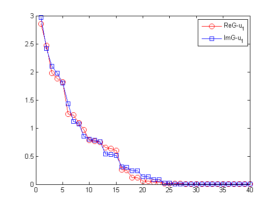
Fig. 1: Singular values of the Fredholm integral equations for the reconstruction of 𝒈𝒈\boldsymbol{g}: (left) component for u1subscript𝑢1u_{1}; (right) component for u2subscript𝑢2u_{2}.

It is known that Fredholm integral equations of the first kind are ill-posed due to the rapidly decaying singular values of matrices from the discretized integral kernels. Appropriate regularization methods are needed to recover the information about the solutions as stably as possible. As a representative example, Figure 1 plots the singular values of the matrices for the Fredholm integral equations (18)–(21) at ω=1.9π𝜔1.9𝜋\omega=1.9\pi. We can observe similar decaying patterns for the singular values of (18) and (20) for the component u1subscript𝑢1u_{1}, and of (19) and (21) for the component u2subscript𝑢2u_{2}.

To reconstruct the variance 𝒉2superscript𝒉2\boldsymbol{h}^{2}, we use Proposition 6 to obtain

𝐄(|DRe𝔾(x,y,ωk)𝒉(y)dWy|2)=DRe𝔾(x,y,ωk)𝒉(y)2dy=D[(GRe[11](x,y,ωk))2+(GRe[21](x,y,ωk))2]h12(y)dy+D[(GRe[12](x,y,ωk))2+(GRe[22](x,y,ωk))2]h22(y)dy𝐄superscriptsubscript𝐷Re𝔾𝑥𝑦subscript𝜔𝑘𝒉𝑦differential-dsubscript𝑊𝑦2subscript𝐷superscriptdelimited-∥∥Re𝔾𝑥𝑦subscript𝜔𝑘𝒉𝑦2differential-d𝑦subscript𝐷delimited-[]superscriptsuperscriptsubscript𝐺Redelimited-[]11𝑥𝑦subscript𝜔𝑘2superscriptsuperscriptsubscript𝐺Redelimited-[]21𝑥𝑦subscript𝜔𝑘2superscriptsubscript12𝑦differential-d𝑦subscript𝐷delimited-[]superscriptsuperscriptsubscript𝐺Redelimited-[]12𝑥𝑦subscript𝜔𝑘2superscriptsuperscriptsubscript𝐺Redelimited-[]22𝑥𝑦subscript𝜔𝑘2superscriptsubscript22𝑦differential-d𝑦\begin{split}&{\bf E}\Bigl{(}\Bigl{|}\int_{D}{\rm Re}\mathbb{G}(x,y,\omega_{k})\boldsymbol{h}(y){\rm d}W_{y}\Bigr{|}^{2}\Bigr{)}=\int_{D}\|{\rm Re}\mathbb{G}(x,y,\omega_{k})\boldsymbol{h}(y)\|^{2}{\rm d}y\\ =&\int_{D}\Big{[}(G_{\rm Re}^{[11]}(x,y,\omega_{k}))^{2}+(G_{\rm Re}^{[21]}(x,y,\omega_{k}))^{2}\Big{]}h_{1}^{2}(y){\rm d}y\\ &+\int_{D}\Big{[}(G_{\rm Re}^{[12]}(x,y,\omega_{k}))^{2}+(G_{\rm Re}^{[22]}(x,y,\omega_{k}))^{2}\Big{]}h_{2}^{2}(y){\rm d}y\end{split}

and

𝐄(|DIm𝔾(x,y,ωk)𝒉(y)dWy|2)=DIm𝔾(x,y,ωk)𝒉(y)2dy=D[(GIm[11](x,y,ωk))2+(GIm[21](x,y,ωk))2]h12(y)dy+D[(GIm[12](x,y,ωk))2+(GIm[22](x,y,ωk))2]h22(y)dy.𝐄superscriptsubscript𝐷Im𝔾𝑥𝑦subscript𝜔𝑘𝒉𝑦differential-dsubscript𝑊𝑦2subscript𝐷superscriptdelimited-∥∥Im𝔾𝑥𝑦subscript𝜔𝑘𝒉𝑦2differential-d𝑦subscript𝐷delimited-[]superscriptsuperscriptsubscript𝐺Imdelimited-[]11𝑥𝑦subscript𝜔𝑘2superscriptsuperscriptsubscript𝐺Imdelimited-[]21𝑥𝑦subscript𝜔𝑘2superscriptsubscript12𝑦differential-d𝑦subscript𝐷delimited-[]superscriptsuperscriptsubscript𝐺Imdelimited-[]12𝑥𝑦subscript𝜔𝑘2superscriptsuperscriptsubscript𝐺Imdelimited-[]22𝑥𝑦subscript𝜔𝑘2superscriptsubscript22𝑦differential-d𝑦\begin{split}&{\bf E}\Bigl{(}\Bigl{|}\int_{D}{\rm Im}\mathbb{G}(x,y,\omega_{k})\boldsymbol{h}(y){\rm d}W_{y}\Bigr{|}^{2}\Bigr{)}=\int_{D}\|{\rm Im}\mathbb{G}(x,y,\omega_{k})\boldsymbol{h}(y)\|^{2}{\rm d}y\\ =&\int_{D}\Big{[}(G_{\rm Im}^{[11]}(x,y,\omega_{k}))^{2}+(G_{\rm Im}^{[21]}(x,y,\omega_{k}))^{2}\Big{]}h_{1}^{2}(y){\rm d}y\\ &+\int_{D}\Big{[}(G_{\rm Im}^{[12]}(x,y,\omega_{k}))^{2}+(G_{\rm Im}^{[22]}(x,y,\omega_{k}))^{2}\Big{]}h_{2}^{2}(y){\rm d}y.\end{split}

Taking the variance on both sides of (16) and (17), we get

𝐕(Re𝒖(x,ωk))=𝐕Re𝒖𝑥subscript𝜔𝑘absent\displaystyle{\bf V}({\rm Re}\boldsymbol{u}(x,\omega_{k}))= D[(GRe[11](x,y,ωk))2+(GRe[21](x,y,ωk))2]h12(y)dysubscript𝐷delimited-[]superscriptsuperscriptsubscript𝐺Redelimited-[]11𝑥𝑦subscript𝜔𝑘2superscriptsuperscriptsubscript𝐺Redelimited-[]21𝑥𝑦subscript𝜔𝑘2superscriptsubscript12𝑦differential-d𝑦\displaystyle\int_{D}\Big{[}(G_{\rm Re}^{[11]}(x,y,\omega_{k}))^{2}+(G_{\rm Re}^{[21]}(x,y,\omega_{k}))^{2}\Big{]}h_{1}^{2}(y){\rm d}y
+D[(GRe[12](x,y,ωk))2+(GRe[22](x,y,ωk))2]h22(y)dy,subscript𝐷delimited-[]superscriptsuperscriptsubscript𝐺Redelimited-[]12𝑥𝑦subscript𝜔𝑘2superscriptsuperscriptsubscript𝐺Redelimited-[]22𝑥𝑦subscript𝜔𝑘2superscriptsubscript22𝑦differential-d𝑦\displaystyle+\int_{D}\Big{[}(G_{\rm Re}^{[12]}(x,y,\omega_{k}))^{2}+(G_{\rm Re}^{[22]}(x,y,\omega_{k}))^{2}\Big{]}h_{2}^{2}(y){\rm d}y,
𝐕(Im𝒖(x,ωk))=𝐕Im𝒖𝑥subscript𝜔𝑘absent\displaystyle{\bf V}({\rm Im}\boldsymbol{u}(x,\omega_{k}))= D[(GIm[11](x,y,ωk))2+(GIm[21](x,y,ωk))2]h12(y)dysubscript𝐷delimited-[]superscriptsuperscriptsubscript𝐺Imdelimited-[]11𝑥𝑦subscript𝜔𝑘2superscriptsuperscriptsubscript𝐺Imdelimited-[]21𝑥𝑦subscript𝜔𝑘2superscriptsubscript12𝑦differential-d𝑦\displaystyle\int_{D}\Big{[}(G_{\rm Im}^{[11]}(x,y,\omega_{k}))^{2}+(G_{\rm Im}^{[21]}(x,y,\omega_{k}))^{2}\Big{]}h_{1}^{2}(y){\rm d}y
+D[(GIm[12](x,y,ωk))2+(GIm[22](x,y,ωk))2]h22(y)dy,subscript𝐷delimited-[]superscriptsuperscriptsubscript𝐺Imdelimited-[]12𝑥𝑦subscript𝜔𝑘2superscriptsuperscriptsubscript𝐺Imdelimited-[]22𝑥𝑦subscript𝜔𝑘2superscriptsubscript22𝑦differential-d𝑦\displaystyle+\int_{D}\Big{[}(G_{\rm Im}^{[12]}(x,y,\omega_{k}))^{2}+(G_{\rm Im}^{[22]}(x,y,\omega_{k}))^{2}\Big{]}h_{2}^{2}(y){\rm d}y,

which are the Fredholm integral equations of the first kind to reconstruct the variance. Again, we consider the variance of components u1subscript𝑢1u_{1} and u2subscript𝑢2u_{2}:

(22) 𝐕(Reu1(x,ωk))𝐕Resubscript𝑢1𝑥subscript𝜔𝑘\displaystyle{\bf V}({\rm Re}u_{1}(x,\omega_{k})) =D[(GRe[11](x,y,ωk))2h12(y)+(GRe[12](x,y,ωk))2h22(y)]dy,absentsubscript𝐷delimited-[]superscriptsuperscriptsubscript𝐺Redelimited-[]11𝑥𝑦subscript𝜔𝑘2superscriptsubscript12𝑦superscriptsuperscriptsubscript𝐺Redelimited-[]12𝑥𝑦subscript𝜔𝑘2superscriptsubscript22𝑦differential-d𝑦\displaystyle=\int_{D}\Big{[}\big{(}G_{\rm Re}^{[11]}(x,y,\omega_{k})\big{)}^{2}h_{1}^{2}(y)+\big{(}G_{\rm Re}^{[12]}(x,y,\omega_{k})\big{)}^{2}h_{2}^{2}(y)\Big{]}{\rm d}y,
(23) 𝐕(Reu2(x,ωk))𝐕Resubscript𝑢2𝑥subscript𝜔𝑘\displaystyle{\bf V}({\rm Re}u_{2}(x,\omega_{k})) =D[(GRe[21](x,y,ωk))2h12(y)+(GRe[22](x,y,ωk))2h22(y)]dy,absentsubscript𝐷delimited-[]superscriptsuperscriptsubscript𝐺Redelimited-[]21𝑥𝑦subscript𝜔𝑘2superscriptsubscript12𝑦superscriptsuperscriptsubscript𝐺Redelimited-[]22𝑥𝑦subscript𝜔𝑘2superscriptsubscript22𝑦differential-d𝑦\displaystyle=\int_{D}\Big{[}\big{(}G_{\rm Re}^{[21]}(x,y,\omega_{k})\big{)}^{2}h_{1}^{2}(y)+\big{(}G_{\rm Re}^{[22]}(x,y,\omega_{k})\big{)}^{2}h_{2}^{2}(y)\Big{]}{\rm d}y,
(24) 𝐕(Imu1(x,ωk))𝐕Imsubscript𝑢1𝑥subscript𝜔𝑘\displaystyle{\bf V}({\rm Im}u_{1}(x,\omega_{k})) =D[(GIm[11](x,y,ωk))2h12(y)+(GIm[12](x,y,ωk))2h22(y)]dy,absentsubscript𝐷delimited-[]superscriptsuperscriptsubscript𝐺Imdelimited-[]11𝑥𝑦subscript𝜔𝑘2superscriptsubscript12𝑦superscriptsuperscriptsubscript𝐺Imdelimited-[]12𝑥𝑦subscript𝜔𝑘2superscriptsubscript22𝑦differential-d𝑦\displaystyle=\int_{D}\Big{[}\big{(}G_{\rm Im}^{[11]}(x,y,\omega_{k})\big{)}^{2}h_{1}^{2}(y)+\big{(}G_{\rm Im}^{[12]}(x,y,\omega_{k})\big{)}^{2}h_{2}^{2}(y)\Big{]}{\rm d}y,
(25) 𝐕(Imu2(x,ωk))𝐕Imsubscript𝑢2𝑥subscript𝜔𝑘\displaystyle{\bf V}({\rm Im}u_{2}(x,\omega_{k})) =D[(GIm[21](x,y,ωk))2h12(y)+(GIm[22](x,y,ωk))2h22(y)]dy.absentsubscript𝐷delimited-[]superscriptsuperscriptsubscript𝐺Imdelimited-[]21𝑥𝑦subscript𝜔𝑘2superscriptsubscript12𝑦superscriptsuperscriptsubscript𝐺Imdelimited-[]22𝑥𝑦subscript𝜔𝑘2superscriptsubscript22𝑦differential-d𝑦\displaystyle=\int_{D}\Big{[}\big{(}G_{\rm Im}^{[21]}(x,y,\omega_{k})\big{)}^{2}h_{1}^{2}(y)+\big{(}G_{\rm Im}^{[22]}(x,y,\omega_{k})\big{)}^{2}h_{2}^{2}(y)\Big{]}{\rm d}y.

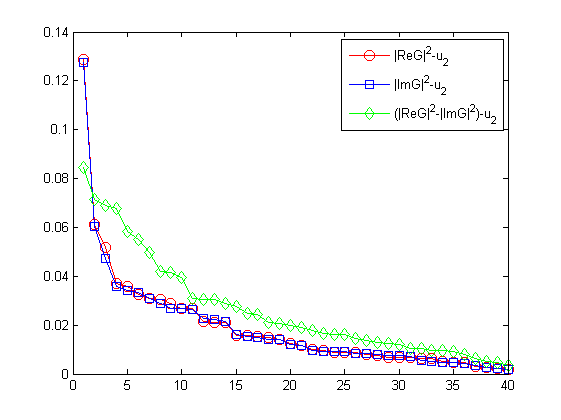
To investigate ill-posedness of the above four equations, we plot their singular values in Figure 2. It can be seen that (22), (24) and (23), (25) show almost identical distributions of the singular values for components u1subscript𝑢1u_{1} and u2subscript𝑢2u_{2}, respectively. The singular values decay exponentially to zeros and there is a big gap between the few leading singular values and the rests. Hence it is severely ill-posed to use directly either (22) or (24) and (23) or (25) to reconstruct h12superscriptsubscript12h_{1}^{2} and h22superscriptsubscript22h_{2}^{2}. Subtracting (24) from (22) and (25) from (23), we obtain the improved equations to reconstruct h12superscriptsubscript12h_{1}^{2} and h22superscriptsubscript22h_{2}^{2}:

𝐕(Reu1(x,ωk))𝐕(Imu1(x,ωk))=D[(GRe[11](x,y,ωk))2(GIm[11](x,y,ωk))2]h12(y)dy𝐕Resubscript𝑢1𝑥subscript𝜔𝑘𝐕Imsubscript𝑢1𝑥subscript𝜔𝑘subscript𝐷delimited-[]superscriptsuperscriptsubscript𝐺Redelimited-[]11𝑥𝑦subscript𝜔𝑘2superscriptsuperscriptsubscript𝐺Imdelimited-[]11𝑥𝑦subscript𝜔𝑘2superscriptsubscript12𝑦differential-d𝑦\displaystyle{\bf V}({\rm Re}u_{1}(x,\omega_{k}))-{\bf V}({\rm Im}u_{1}(x,\omega_{k}))=\int_{D}\Big{[}\big{(}G_{\rm Re}^{[11]}(x,y,\omega_{k})\big{)}^{2}-\big{(}G_{\rm Im}^{[11]}(x,y,\omega_{k})\big{)}^{2}\Big{]}h_{1}^{2}(y){\rm d}y
(26) +D[(GRe[12](x,y,ωk))2(GIm[12](x,y,ωk))2]h22(y)dy,subscript𝐷delimited-[]superscriptsuperscriptsubscript𝐺Redelimited-[]12𝑥𝑦subscript𝜔𝑘2superscriptsuperscriptsubscript𝐺Imdelimited-[]12𝑥𝑦subscript𝜔𝑘2superscriptsubscript22𝑦differential-d𝑦\displaystyle+\int_{D}\Big{[}\big{(}G_{\rm Re}^{[12]}(x,y,\omega_{k})\big{)}^{2}-\big{(}G_{\rm Im}^{[12]}(x,y,\omega_{k})\big{)}^{2}\Big{]}h_{2}^{2}(y){\rm d}y,
𝐕(Reu2(x,ωk))𝐕(Imu2(x,ωk))=D[(GRe[21](x,y,ωk))2(GIm[21](x,y,ωk))2]h12(y)dy𝐕Resubscript𝑢2𝑥subscript𝜔𝑘𝐕Imsubscript𝑢2𝑥subscript𝜔𝑘subscript𝐷delimited-[]superscriptsuperscriptsubscript𝐺Redelimited-[]21𝑥𝑦subscript𝜔𝑘2superscriptsuperscriptsubscript𝐺Imdelimited-[]21𝑥𝑦subscript𝜔𝑘2superscriptsubscript12𝑦differential-d𝑦\displaystyle{\bf V}({\rm Re}u_{2}(x,\omega_{k}))-{\bf V}({\rm Im}u_{2}(x,\omega_{k}))=\int_{D}\Big{[}\big{(}G_{\rm Re}^{[21]}(x,y,\omega_{k})\big{)}^{2}-\big{(}G_{\rm Im}^{[21]}(x,y,\omega_{k})\big{)}^{2}\Big{]}h_{1}^{2}(y){\rm d}y
(27) +D[(GRe[22](x,y,ωk))2(GIm[22](x,y,ωk))2]h22(y)dy.subscript𝐷delimited-[]superscriptsuperscriptsubscript𝐺Redelimited-[]22𝑥𝑦subscript𝜔𝑘2superscriptsuperscriptsubscript𝐺Imdelimited-[]22𝑥𝑦subscript𝜔𝑘2superscriptsubscript22𝑦differential-d𝑦\displaystyle+\int_{D}\Big{[}\big{(}G_{\rm Re}^{[22]}(x,y,\omega_{k})\big{)}^{2}-\big{(}G_{\rm Im}^{[22]}(x,y,\omega_{k})\big{)}^{2}\Big{]}h_{2}^{2}(y){\rm d}y.

In fact, it is clear to note in Figure 2 that the singular values of (3.1) and (3.1) display better behavior that those of (22), (24) and (23), (25). The singular values decay more slowly and distribute more uniformly. Numerically, (3.1) and (3.1) do give much better reconstructions. We will only show the results for (3.1) and (3.1) in the numerical experiments.

Refer to caption
Refer to caption
Fig. 2: Singular values of the Fredholm integral equations for the reconstruction of 𝒉2superscript𝒉2\boldsymbol{h}^{2}: (left) component of u1subscript𝑢1u_{1}; (right) component of u2subscript𝑢2u_{2}.

3.2 Numerical method

In this section, we present a regularized Kaczmarz method to solve the ill-posed integral equations. The classical Kaczmarz method is an iterative method for solving linear systems of algebraic equations [30].

Consider the following operator equations

(28) Akq=pk,k=1,,K,formulae-sequencesubscript𝐴𝑘𝑞subscript𝑝𝑘𝑘1𝐾A_{k}q=p_{k},\quad k=1,\dots,K,

where the index k𝑘k is for different frequency, q𝑞q represents the unknown g1,g2subscript𝑔1subscript𝑔2g_{1},g_{2} or h12,h22superscriptsubscript12superscriptsubscript22h_{1}^{2},h_{2}^{2}, and pksubscript𝑝𝑘p_{k} is the given data. Given an arbitrary initial guess q0superscript𝑞0q^{0}, the classical Kaczmarz method for solving (28) reads: For l=0,1,,L𝑙01𝐿l=0,1,\dots,L,

(29) {q0=ql,qk=qk1+Ak(AkAk)1(pkAkqk1),k=1,,K,ql+1=qK,casessubscript𝑞0superscript𝑞𝑙otherwiseformulae-sequencesubscript𝑞𝑘subscript𝑞𝑘1subscriptsuperscript𝐴𝑘superscriptsubscript𝐴𝑘subscriptsuperscript𝐴𝑘1subscript𝑝𝑘subscript𝐴𝑘subscript𝑞𝑘1𝑘1𝐾otherwisesuperscript𝑞𝑙1subscript𝑞𝐾otherwise\begin{cases}q_{0}=q^{l},\\ q_{k}=q_{k-1}+A^{*}_{k}(A_{k}A^{*}_{k})^{-1}(p_{k}-A_{k}q_{k-1}),\quad k=1,\dots,K,\\ q^{l+1}=q_{K},\end{cases}

where Aksuperscriptsubscript𝐴𝑘A_{k}^{*} is the adjoint operator of Aksubscript𝐴𝑘A_{k}. In (29), there are two loops: the outer loop is carried for iterative index l𝑙l and the inner loop is done for the different frequency ωksubscript𝜔𝑘\omega_{k}. In practice, the operator AkAksubscript𝐴𝑘subscriptsuperscript𝐴𝑘A_{k}A^{*}_{k} may not be invertible or is bad conditioned even if it is invertible. A regularization technique is needed.

We present a regularized Kaczmarz method: Given an arbitrary initial guess q0superscript𝑞0q^{0},

(30) {q0=ql,qk=qk1+Ak(γI+AkAk)1(pkAkqk1),k=1,,K,ql+1=qm,casessubscript𝑞0superscript𝑞𝑙otherwiseformulae-sequencesubscript𝑞𝑘subscript𝑞𝑘1subscriptsuperscript𝐴𝑘superscript𝛾𝐼subscript𝐴𝑘subscriptsuperscript𝐴𝑘1subscript𝑝𝑘subscript𝐴𝑘subscript𝑞𝑘1𝑘1𝐾otherwisesuperscript𝑞𝑙1subscript𝑞𝑚otherwise\begin{cases}q_{0}=q^{l},\\ q_{k}=q_{k-1}+A^{*}_{k}(\gamma I+A_{k}A^{*}_{k})^{-1}(p_{k}-A_{k}q_{k-1}),\quad k=1,\dots,K,\\ q^{l+1}=q_{m},\end{cases}

for l=0,1,,L𝑙01𝐿l=0,1,\dots,L, where γ>0𝛾0\gamma>0 is the regularization parameter and I𝐼I is the identity operator. Although there are two loops in (30), the operator γI+AkAk𝛾𝐼subscript𝐴𝑘subscriptsuperscript𝐴𝑘\gamma I+A_{k}A^{*}_{k} leads to a small scale linear system of equations with the size equal to the number of measurements. Moreover, they essentially need to be solved only K𝐾K times by a direct solver such as the LU decomposition since Aksubscript𝐴𝑘A_{k} keep the same during the outer loop.

4 Numerical experiments

In this section, we present a numerical example to demonstrate the validity and effectiveness of the proposed method. The scattering data is obtained by the numerical solution of the stochastic Navier equation instead of the numerical integration of the Fredholm integral equations in order to avoid the so-called inverse crime. Although the stochastic Navier equation may be efficiently solved by using the Wiener Chaos expansions to obtain statistical moments such as the mean and variance [4], we choose the Monte Carlo method to simulate the actual process of measuring data. In each realization, the stochastic Navier equation is solved by using the finite element method with the perfectly matched layer (PML) technique. After all the realizations are done, we take an average of the solutions and use it as an approximated scattering data to either the mean or the variance. It is clear to note that the data is more accurate as more number of realizations is taken.
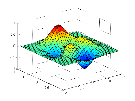
Refer to caption
Refer to caption
Refer to caption
Refer to caption
Fig. 3: The exact source: (top) surface plot of the exact mean g1subscript𝑔1g_{1} and g2subscript𝑔2g_{2}; (below) surface plot of the exact variance h12superscriptsubscript12h_{1}^{2} and h22superscriptsubscript22h_{2}^{2}.

Let

g1(x1,x2)=0.3(1x1)2ex12(x2+1)2(0.2x1x13x25)ex12x220.03e(x1+1)2x22subscript𝑔1subscript𝑥1subscript𝑥20.3superscript1subscript𝑥12superscript𝑒superscriptsubscript𝑥12superscriptsubscript𝑥2120.2subscript𝑥1superscriptsubscript𝑥13superscriptsubscript𝑥25superscript𝑒superscriptsubscript𝑥12superscriptsubscript𝑥220.03superscript𝑒superscriptsubscript𝑥112superscriptsubscript𝑥22g_{1}(x_{1},x_{2})=0.3(1-x_{1})^{2}e^{-x_{1}^{2}-(x_{2}+1)^{2}}-(0.2x_{1}-x_{1}^{3}-x_{2}^{5})e^{-x_{1}^{2}-x_{2}^{2}}-0.03e^{-(x_{1}+1)^{2}-x_{2}^{2}}

and

g2(x1,x2)=5x12x2ex12x22.subscript𝑔2subscript𝑥1subscript𝑥25superscriptsubscript𝑥12subscript𝑥2superscript𝑒superscriptsubscript𝑥12superscriptsubscript𝑥22g_{2}(x_{1},x_{2})=5x_{1}^{2}x_{2}e^{-x_{1}^{2}-x_{2}^{2}}.

We reconstruct the mean 𝒈𝒈\boldsymbol{g} given by

𝒈(x1,x2)=(g1(3x1,3x2),g2(3x1,3x2))𝒈subscript𝑥1subscript𝑥2superscriptsubscript𝑔13subscript𝑥13subscript𝑥2subscript𝑔23subscript𝑥13subscript𝑥2top\boldsymbol{g}(x_{1},x_{2})=(g_{1}(3x_{1},3x_{2}),g_{2}(3x_{1},3x_{2}))^{\top}

inside the domain D=[1, 1]×[1, 1]𝐷1111D=[-1,\,1]\times[-1,\,1]. Let

h1(x1,x2)=0.6e8(r30.75r2)subscript1subscript𝑥1subscript𝑥20.6superscript𝑒8superscript𝑟30.75superscript𝑟2h_{1}(x_{1},x_{2})=0.6e^{-8(r^{3}-0.75r^{2})}

and

h2(x1,x2)=er2,r=(x12+x22)1/2.formulae-sequencesubscript2subscript𝑥1subscript𝑥2superscript𝑒superscript𝑟2𝑟superscriptsuperscriptsubscript𝑥12superscriptsubscript𝑥2212h_{2}(x_{1},x_{2})=e^{-r^{2}},\quad r=(x_{1}^{2}+x_{2}^{2})^{1/2}.

We reconstruct the variance 𝒉2superscript𝒉2\boldsymbol{h}^{2} given by

𝒉2(x1,x2)=[h12(x1,x2)00h22(3x1,3x2)]superscript𝒉2subscript𝑥1subscript𝑥2matrixsubscriptsuperscript21subscript𝑥1subscript𝑥200subscriptsuperscript223subscript𝑥13subscript𝑥2\boldsymbol{h}^{2}(x_{1},x_{2})=\begin{bmatrix}h^{2}_{1}(x_{1},x_{2})&0\\ 0&h^{2}_{2}(3x_{1},3x_{2})\end{bmatrix}

inside the domain D=[1, 1]×[1, 1]𝐷1111D=[-1,\,1]\times[-1,\,1]. See Figure 3 for the surface plot of the exact g1,g2subscript𝑔1subscript𝑔2g_{1},g_{2} (top) and h12,h22superscriptsubscript12superscriptsubscript22h_{1}^{2},h_{2}^{2} (below). The Lamé constants are μ=1.0𝜇1.0\mu=1.0 and λ=2.0𝜆2.0\lambda=2.0. The computational domain is set to be [3, 3]×[3, 3]3333[-3,\,3]\times[-3,\,3] with the PML thickness 0.50.50.5. After the direct problem is solved and the value of 𝒖𝒖\boldsymbol{u} is obtained at the grid points, the linear interpolation is used to generate the synthetic data at 40 uniformly distributed points on the circle with radius 2, i.e., x1=2cosθi,x2=2sinθi,θi=iπ/20,i=0,1,,39.formulae-sequencesubscript𝑥12subscript𝜃𝑖formulae-sequencesubscript𝑥22subscript𝜃𝑖formulae-sequencesubscript𝜃𝑖𝑖𝜋20𝑖0139x_{1}=2\cos\theta_{i},x_{2}=2\sin\theta_{i},\theta_{i}=i\pi/20,i=0,1,\dots,39. Sixteen equally spaced frequencies from 0.5π0.5𝜋0.5\pi to 7.5π7.5𝜋7.5\pi are used in the reconstruction of g1,g2subscript𝑔1subscript𝑔2g_{1},g_{2}, while twenty equally spaced frequencies from 0.5π0.5𝜋0.5\pi to 2.5π2.5𝜋2.5\pi are used in the reconstruction of h12,h22superscriptsubscript12superscriptsubscript22h_{1}^{2},h_{2}^{2}. The regularization parameter is γ=1.0×10⁷𝛾1.0superscript107\gamma=1.0\times 10^{-7} and the total number of the outer loop for the Kaczmarz method is L=5𝐿5L=5. Figure 4 shows the reconstructed mean g1,g2subscript𝑔1subscript𝑔2g_{1},g_{2} (top) and the reconstructed variance h12,h22superscriptsubscript12superscriptsubscript22h_{1}^{2},h_{2}^{2} (below) corresponding to the number of realization 104superscript10410^{4}.

Refer to caption
Refer to caption
Refer to caption
Refer to caption
Fig. 4: The reconstructed source: (top) surface plot of the reconstructed mean g1,g2subscript𝑔1subscript𝑔2g_{1},g_{2}; (below) surface plot of the reconstructed variance h12,h22superscriptsubscript12superscriptsubscript22h_{1}^{2},h_{2}^{2}.

5 Conclusion

We have studied the direct and inverse random source scattering problems for the stochastic Navier equation where the source is driven by an additive white noise. Under a suitable regularity assumption of the source functions 𝒈𝒈\boldsymbol{g} and 𝒉𝒉\boldsymbol{h}, the direct scattering problem is shown constructively to have a unique mild solution which was given explicitly as an integral equation. Based on the explicit solution, Fredholm integral equations are deduced for the inverse scattering problem to reconstruct the mean and the variance of the random source. We have presented the regularized Kaczmarz method to solve the ill-posed integral equations by using multiple frequency data. A numerical example is presented to demonstrate the validity and effectiveness of the proposed method. We are currently investigating the inverse random source scattering problem in an inhomogeneous elastic medium where the explicit Green tensor function is no longer available. Although this paper concerns the inverse random source scattering problem for the Navier equation, we believe that the proposed framework and methodology can be directly applied to solve many other inverse random source problems and even more general stochastic inverse problems. For instance, it is interesting to study inverse random source problems for the stochastic Poisson, heat, or electromagnetic wave equation. Obviously, it is more challenging to consider the inverse random medium scattering problem where the medium should be modeled as a random function. We hope to be able to report the progress on these problems in the future.

Appendix A Brownian sheet

Let us first briefly introduce the one-dimensional Brownian sheet, which is also called one-dimensional d𝑑d-parameter Brownian motion, on (+d,(+d),μ)subscriptsuperscript𝑑subscriptsuperscript𝑑𝜇(\mathbb{R}^{d}_{+},\,\mathcal{B}(\mathbb{R}^{d}_{+}),\,\mu), where d,+d={x=(x1,,xd)d:xj0,j=1,,d}formulae-sequence𝑑superscriptsubscript𝑑conditional-set𝑥superscriptsubscript𝑥1subscript𝑥𝑑topsuperscript𝑑formulae-sequencesubscript𝑥𝑗0𝑗1𝑑d\in\mathbb{N},\mathbb{R}_{+}^{d}=\{x=(x_{1},\dots,x_{d})^{\top}\in\mathbb{R}^{d}:x_{j}\geq 0,j=1,\dots,d\}, (+d)subscriptsuperscript𝑑\mathcal{B}(\mathbb{R}^{d}_{+}) is the Borel σ𝜎\sigma-algebra of +dsubscriptsuperscript𝑑\mathbb{R}^{d}_{+}, and μ𝜇\mu is the Lebesgue measure. More details can be found in [31]. Let (0,x]=(0,x1]××(0,xd]0𝑥0subscript𝑥10subscript𝑥𝑑(0,x]=(0,x_{1}]\times\cdots\times(0,x_{d}] for x+d𝑥subscriptsuperscript𝑑x\in\mathbb{R}^{d}_{+}.

Definition 4.

The one-dimensional Brownian sheet on +dsubscriptsuperscript𝑑\mathbb{R}^{d}_{+} is the process {Wx:x+d}conditional-setsubscript𝑊𝑥𝑥subscriptsuperscript𝑑\{W_{x}:x\in\mathbb{R}^{d}_{+}\} defined by Wx=W{(0,x]}subscript𝑊𝑥𝑊0𝑥W_{x}=W\{(0,x]\}, where W𝑊W is a random set function such that

  1. 1.

    A(+d)for-all𝐴subscriptsuperscript𝑑\forall A\in\mathcal{B}(\mathbb{R}^{d}_{+}), W(A)𝑊𝐴W(A) is a Gaussian random variable with mean 0 and variance μ(A)𝜇𝐴\mu(A), i.e., W(A)𝒩(0,μ(A))similar-to𝑊𝐴𝒩0𝜇𝐴W(A)\sim\mathcal{N}(0,\mu(A));

  2. 2.

    A,B(+d)for-all𝐴𝐵subscriptsuperscript𝑑\forall A,B\in\mathcal{B}(\mathbb{R}^{d}_{+}), if AB=𝐴𝐵A\cap B=\emptyset, then W(A)𝑊𝐴W(A) and W(B)𝑊𝐵W(B) are independent and W(AB)=W(A)+W(B)𝑊𝐴𝐵𝑊𝐴𝑊𝐵W(A\cup B)=W(A)+W(B).

It can be verified from Definition 4 that

𝐄(W(A)W(B))=μ(AB),A,B(+d),formulae-sequence𝐄𝑊𝐴𝑊𝐵𝜇𝐴𝐵for-all𝐴𝐵subscriptsuperscript𝑑{\bf E}(W(A)W(B))=\mu(A\cap B),\quad\forall A,B\in\mathcal{B}(\mathbb{R}^{d}_{+}),

which gives the covariance function of the Brownian sheet:

𝐄(WxWy)=xy:=(x1y1)(xdyd)𝐄subscript𝑊𝑥subscript𝑊𝑦𝑥𝑦assignsubscript𝑥1subscript𝑦1subscript𝑥𝑑subscript𝑦𝑑{\bf E}(W_{x}W_{y})=x\wedge y:=(x_{1}\wedge y_{1})\cdots(x_{d}\wedge y_{d})

for any x=(x1,,xd)+d𝑥superscriptsubscript𝑥1subscript𝑥𝑑topsubscriptsuperscript𝑑x=(x_{1},\dots,x_{d})^{\top}\in\mathbb{R}^{d}_{+} and y=(y1,,yd)+d𝑦superscriptsubscript𝑦1subscript𝑦𝑑topsubscriptsuperscript𝑑y=(y_{1},\dots,y_{d})^{\top}\in\mathbb{R}^{d}_{+}, where xjyj=min{xj,yj}subscript𝑥𝑗subscript𝑦𝑗subscript𝑥𝑗subscript𝑦𝑗x_{j}\wedge y_{j}=\min\{x_{j},\,y_{j}\}.

The Brownian sheet can be generalized to the space dsuperscript𝑑\mathbb{R}^{d} by introducing 2dsuperscript2𝑑2^{d} independent Brownian sheets defined on +dsubscriptsuperscript𝑑\mathbb{R}^{d}_{+}. Define a multi-index t=(t1,,td)𝑡superscriptsubscript𝑡1subscript𝑡𝑑topt=(t_{1},\dots,t_{d})^{\top} with tj={1,1}subscript𝑡𝑗11t_{j}=\{1,\,-1\} for j=1,,d𝑗1𝑑j=1,\dots,d. Introduce 2dsuperscript2𝑑2^{d} independent Brownian sheets {Wt}superscript𝑊𝑡\{W^{t}\} defined on +dsubscriptsuperscript𝑑\mathbb{R}^{d}_{+}. For any x=(x1,,xd)d𝑥superscriptsubscript𝑥1subscript𝑥𝑑topsuperscript𝑑x=(x_{1},\dots,x_{d})^{\top}\in\mathbb{R}^{d}, define the Brownian sheet

Wx:=Wx˘t(x),assignsubscript𝑊𝑥subscriptsuperscript𝑊𝑡𝑥˘𝑥W_{x}:=W^{t(x)}_{\breve{x}},

where x˘=(|x1|,,|xd|)˘𝑥superscriptsubscript𝑥1subscript𝑥𝑑top\breve{x}=(|x_{1}|,\dots,|x_{d}|)^{\top} and t(x)=(sgn(x1),,sgn(xd))𝑡𝑥superscriptsgnsubscript𝑥1sgnsubscript𝑥𝑑topt(x)=({\rm sgn}(x_{1}),\dots,{\rm sgn}(x_{d}))^{\top}. The sign function sgn(xj)=1sgnsubscript𝑥𝑗1{\rm sgn}(x_{j})=1 if xj0subscript𝑥𝑗0x_{j}\geq 0, otherwise sgn(xj)=1sgnsubscript𝑥𝑗1{\rm sgn}(x_{j})=-1.

In two or more parameters, the white noise can be thought of as the derivative of the Brownian sheet. In fact, the Brownian sheet Wxsubscript𝑊𝑥W_{x} is nowhere-differentiable in the ordinary sense, but its derivatives will exist in the sense of Schwartz distributions. Define

W˙x=dWxx1xd.subscript˙𝑊𝑥superscript𝑑subscript𝑊𝑥subscript𝑥1subscript𝑥𝑑\dot{W}_{x}=\frac{\partial^{d}W_{x}}{\partial x_{1}\cdots\partial x_{d}}.

If ϕ(x)italic-ϕ𝑥\phi(x) is a deterministic square-integrable complex-valued test function with a compact support in dsuperscript𝑑\mathbb{R}^{d}, then W˙xsubscript˙𝑊𝑥\dot{W}_{x} is the distribution

W˙x(ϕ)=(1)ddWxdϕ(x)x1xddx.subscript˙𝑊𝑥italic-ϕsuperscript1𝑑subscriptsuperscript𝑑subscript𝑊𝑥superscript𝑑italic-ϕ𝑥subscript𝑥1subscript𝑥𝑑differential-d𝑥\dot{W}_{x}(\phi)=(-1)^{d}\int_{\mathbb{R}^{d}}W_{x}\frac{\partial^{d}\phi(x)}{\partial x_{1}\cdots\partial x_{d}}{\rm d}x.

We may define the stochastic integral

(31) dϕ(x)dWx=(1)ddWxdϕ(x)x1xddx,subscriptsuperscript𝑑italic-ϕ𝑥differential-dsubscript𝑊𝑥superscript1𝑑subscriptsuperscript𝑑subscript𝑊𝑥superscript𝑑italic-ϕ𝑥subscript𝑥1subscript𝑥𝑑differential-d𝑥\int_{\mathbb{R}^{d}}\phi(x){\rm d}W_{x}=(-1)^{d}\int_{\mathbb{R}^{d}}W_{x}\frac{\partial^{d}\phi(x)}{\partial x_{1}\cdots\partial x_{d}}{\rm d}x,

which satisfies the following properties (cf. [5, Proposition A.2]).

Lemma 5.

Let ϕ(x)italic-ϕ𝑥\phi(x) be a test function with a compact support in dsuperscript𝑑\mathbb{R}^{d}. We have

𝐄(dϕ(x)dWx)=0,𝐄(|dϕ(x)dWx|2)=d|ϕ(x)|2dx.formulae-sequence𝐄subscriptsuperscript𝑑italic-ϕ𝑥differential-dsubscript𝑊𝑥0𝐄superscriptsubscriptsuperscript𝑑italic-ϕ𝑥differential-dsubscript𝑊𝑥2subscriptsuperscript𝑑superscriptitalic-ϕ𝑥2differential-d𝑥{\bf E}\Bigl{(}\int_{\mathbb{R}^{d}}\phi(x){\rm d}W_{x}\Bigr{)}=0,\quad{\bf E}\Bigl{(}\bigl{|}\int_{\mathbb{R}^{d}}\phi(x){\rm d}W_{x}\bigr{|}^{2}\Bigr{)}=\int_{\mathbb{R}^{d}}|\phi(x)|^{2}{\rm d}x.

The stochastic integral (31) can be extended to define the multi-dimensional stochastic integrals. Let W(x)=(W1(x),,Wn(x))𝑊𝑥superscriptsubscript𝑊1𝑥subscript𝑊𝑛𝑥topW(x)=(W_{1}(x),\dots,W_{n}(x))^{\top} be an n𝑛n-dimensional Brownian sheet, where Wi(x)subscript𝑊𝑖𝑥W_{i}(x) and Wj(x)subscript𝑊𝑗𝑥W_{j}(x) are two one-dimensional independent Brownian sheets for ij𝑖𝑗i\neq j. If ϕ(x)italic-ϕ𝑥\phi(x) is a deterministic square-integrable complex-valued m×n𝑚𝑛m\times n matrix-valued test function with each component compactly supported in dsuperscript𝑑\mathbb{R}^{d}, i.e.,

ϕ(x)=[ϕ11(x)ϕ1n(x)ϕm1(x)ϕmn(x)].italic-ϕ𝑥matrixsubscriptitalic-ϕ11𝑥subscriptitalic-ϕ1𝑛𝑥missing-subexpressionsubscriptitalic-ϕ𝑚1𝑥subscriptitalic-ϕ𝑚𝑛𝑥\phi(x)=\begin{bmatrix}\phi_{11}(x)&\cdots&\phi_{1n}(x)\\ \vdots&&\vdots\\ \phi_{m1}(x)&\cdots&\phi_{mn}(x)\end{bmatrix}.

Using the matrix notation, we may define the multi-dimensional stochastic integral

(32) dϕ(x)dW(x)=d[ϕ11(x)ϕ1n(x)ϕm1(x)ϕmn(x)][dW1(x)dWn(x)],subscriptsuperscript𝑑italic-ϕ𝑥differential-d𝑊𝑥subscriptsuperscript𝑑matrixsubscriptitalic-ϕ11𝑥subscriptitalic-ϕ1𝑛𝑥missing-subexpressionsubscriptitalic-ϕ𝑚1𝑥subscriptitalic-ϕ𝑚𝑛𝑥matrixdsubscript𝑊1𝑥dsubscript𝑊𝑛𝑥\int_{{\mathbb{R}}^{d}}\phi(x){\rm d}W(x)=\int_{{\mathbb{R}}^{d}}\begin{bmatrix}\phi_{11}(x)&\cdots&\phi_{1n}(x)\\ \vdots&&\vdots\\ \phi_{m1}(x)&\cdots&\phi_{mn}(x)\end{bmatrix}\begin{bmatrix}{\rm d}W_{1}(x)\\ \vdots\\ {\rm d}W_{n}(x)\end{bmatrix},

which is an m×1𝑚1m\times 1 matrix and its j𝑗j-th component is the sum of 1-dimensional stochastic integrals

k=1ndϕjk(x)dWk(x).superscriptsubscript𝑘1𝑛subscriptsuperscript𝑑subscriptitalic-ϕ𝑗𝑘𝑥differential-dsubscript𝑊𝑘𝑥\sum_{k=1}^{n}\int_{{\mathbb{R}}^{d}}\phi_{jk}(x){\rm d}W_{k}(x).

We have the similar properties for the multi-dimensional stochastic integral.

Proposition 6.

Let W(x)=(W1(x),,Wn(x))𝑊𝑥superscriptsubscript𝑊1𝑥subscript𝑊𝑛𝑥topW(x)=(W_{1}(x),\dots,W_{n}(x))^{\top} be an n𝑛n-dimensional Brownian sheet and ϕ(x)=(ϕij(x))m×nitalic-ϕ𝑥subscriptsubscriptitalic-ϕ𝑖𝑗𝑥𝑚𝑛\phi(x)=(\phi_{ij}(x))_{m\times n} be an m×n𝑚𝑛m\times n matrix-valued function with each component ϕij(x)subscriptitalic-ϕ𝑖𝑗𝑥\phi_{ij}(x) compactly supported in dsuperscript𝑑\mathbb{R}^{d}. We have

𝐄(dϕ(x)dWx)=0,𝐄(|dϕ(x)dWx|2)=dϕ(x)2dx,formulae-sequence𝐄subscriptsuperscript𝑑italic-ϕ𝑥differential-dsubscript𝑊𝑥0𝐄superscriptsubscriptsuperscript𝑑italic-ϕ𝑥differential-dsubscript𝑊𝑥2subscriptsuperscript𝑑superscriptnormitalic-ϕ𝑥2differential-d𝑥{\bf E}\Bigl{(}\int_{\mathbb{R}^{d}}\phi(x){\rm d}W_{x}\Bigr{)}=0,\quad{\bf E}\Bigl{(}\bigl{|}\int_{\mathbb{R}^{d}}\phi(x){\rm d}W_{x}\bigr{|}^{2}\Bigr{)}=\int_{\mathbb{R}^{d}}\|\phi(x)\|^{2}{\rm d}x,

where \|\cdot\| is the Frobenius norm.

Proof.

It follows from (32) and Lemma 5 that

𝐄(dϕ(x)dWx)=[k=1n𝐄(dϕjk(x)dWk(x))k=1n𝐄(dϕjk(x)dWk(x))]=0.𝐄subscriptsuperscript𝑑italic-ϕ𝑥differential-dsubscript𝑊𝑥matrixsuperscriptsubscript𝑘1𝑛𝐄subscriptsuperscript𝑑subscriptitalic-ϕ𝑗𝑘𝑥differential-dsubscript𝑊𝑘𝑥superscriptsubscript𝑘1𝑛𝐄subscriptsuperscript𝑑subscriptitalic-ϕ𝑗𝑘𝑥differential-dsubscript𝑊𝑘𝑥0{\bf E}\Bigl{(}\int_{\mathbb{R}^{d}}\phi(x){\rm d}W_{x}\Bigr{)}=\begin{bmatrix}\sum_{k=1}^{n}{\bf E}\Bigl{(}\int_{{\mathbb{R}}^{d}}\phi_{jk}(x){\rm d}W_{k}(x)\Bigr{)}\\ \vdots\\ \sum_{k=1}^{n}{\bf E}\Bigl{(}\int_{{\mathbb{R}}^{d}}\phi_{jk}(x){\rm d}W_{k}(x)\Bigr{)}\end{bmatrix}=0.

Using (32) and Lemma 5 again, we have

𝐄(|dϕ(x)dWx|2)𝐄superscriptsubscriptsuperscript𝑑italic-ϕ𝑥differential-dsubscript𝑊𝑥2\displaystyle{\bf E}\Bigl{(}\bigl{|}\int_{\mathbb{R}^{d}}\phi(x){\rm d}W_{x}\bigr{|}^{2}\Bigr{)} =j=1m𝐄(|k=1ndϕjk(x)dWk(x)|2)absentsuperscriptsubscript𝑗1𝑚𝐄superscriptsuperscriptsubscript𝑘1𝑛subscriptsuperscript𝑑subscriptitalic-ϕ𝑗𝑘𝑥differential-dsubscript𝑊𝑘𝑥2\displaystyle=\sum_{j=1}^{m}{\bf E}\Bigl{(}\bigl{|}\sum_{k=1}^{n}\int_{\mathbb{R}^{d}}\phi_{jk}(x){\rm d}W_{k}(x)\bigr{|}^{2}\Bigr{)}
=j=1mk=1nd|ϕjk(x)|2dxabsentsuperscriptsubscript𝑗1𝑚superscriptsubscript𝑘1𝑛subscriptsuperscript𝑑superscriptsubscriptitalic-ϕ𝑗𝑘𝑥2differential-d𝑥\displaystyle=\sum_{j=1}^{m}\sum_{k=1}^{n}\int_{\mathbb{R}^{d}}|\phi_{jk}(x)|^{2}{\rm d}x
=dϕ(x)2dx,absentsubscriptsuperscript𝑑superscriptnormitalic-ϕ𝑥2differential-d𝑥\displaystyle=\int_{\mathbb{R}^{d}}\|\phi(x)\|^{2}{\rm d}x,

which completes the proof. ∎

References

  • [1] R. Albanese and P. Monk, The inverse source problem for Maxwell’s equations, Inverse Problems, 22 (2006), 1023–1035.
  • [2] H. Ammari, G. Bao, and J. Fleming, An inverse source problem for Maxwell’s equations in magnetoencephalography, SIAM J. Appl. Math., 62 (2002), 1369–1382.
  • [3] A. Badia and T. Nara, An inverse source problem for Helmholtz’s equation from the Cauchy data with a single wave number, Inverse Problems, 27 (2011), 105001.
  • [4] M. Badieirostami, A. Adibi, H.-M. Zhou, and S.-N. Chow, Wiener chaos expansion and simulation of electromagnetic wave propagation excited by a spatially incoherent source, Multiscale Model. Simul., 8 (2010), pp. 591–604.
  • [5] G. Bao, C. Chen and P. Li, Inverse random source scattering problems in several dimensions, preprint.
  • [6] G. Bao, S.-N. Chow, P. Li, and H.-M. Zhou, An inverse random source problem for the Helmholtz equation, Math. Comp., 83 (2014), 215–233.
  • [7] G. Bao, P. Li, J. Lin, and F. Triki, Inverse scattering problems with multi-frequencies, Inverse Problems, 31 (2015), 093001.
  • [8] G. Bao, J. Lin, and F. Triki, A multi-frequency inverse source problem, J. Differential Equations, 249 (2010), 3443–3465.
  • [9] G. Bao, S. Lu, W. Rundell, and B. Xu, A recursive algorithm for multifrequency acoustic inverse source problems, SIAM J. Numer. Anal., 53 (2015), 1608–1628.
  • [10] G. Bao and X. Xu, An inverse random source problem in quantifying the elastic modulus of nano-materials, Inverse Problems, 29 (2013), 015006.
  • [11] M. Bonnet and A. Constantinescu, Inverse problems in elasticity, Inverse Problems, 21 (2005) 1–50,
  • [12] Y.-Z. Cao, R. Zhang, and K. Zhang, Finite element method and discontinuous Galerkin method for stochastic Helmholtz equation in two- and three-dimensions, J. Comput. Math., 26 (2008), 701–715.
  • [13] D. Colton and R. Kress, Inverse Acoustic and Electromagnetic Scattering Theory, Berlin: Springer, 1998.
  • [14] A. Devaney, The inverse problem for random sources, J. Math. Phys., 20 (1979), 1687–1691.
  • [15] A. Devaney, E. Marengo, and M. Li, Inverse source problem in nonhomogeneous background media, SIAM J. Appl. Math., 67 (2007), 1353–1378.
  • [16] A. Devaney and G. Sherman, Nonuniqueness in inverse source and scattering problems, IEEE Trans. Antennas Propag., 30 (1982), 1034–1037.
  • [17] M. Eller and N. Valdivia, Acoustic source identification using multiple frequency information, Inverse Problems, 25 (2009), 115005.
  • [18] L. Evans, An Introduction to Stochastic Differential Equations, AMS, 2013.
  • [19] A. Fokas, Y. Kurylev, and V. Marinakis, The unique determination of neuronal currents in the brain via magnetoencephalogrphy, Inverse Problems, 20 (2004), 1067–1082.
  • [20] A. Friedman, Stochastic Differential Equations and Applications, New York: Academic Press, 2006.
  • [21] K.-H. Hauer, L. Kühn, and R. Potthast, On uniqueness and non-uniqueness for current reconstruction from magnetic fields, Inverse Problems, 21 (2005), 955–967.
  • [22] M. Hairer, Introduction to Stochastic PDEs, lecture notes, 2009.
  • [23] V. Isakov, Inverse Source Problems, AMS, Providence, RI, 1989.
  • [24] J. Kaipio and E. Somersalo, Statistical and Computational Inverse Problems, Springer-Varlag, New York, 2005.
  • [25] R. Kress, Inverse elastic scattering from a crack, Inverse Problems, 12 (1996), 667–684.
  • [26] L. D. Landau and E. M. Lifshitz, Theory of Elasticity, Oxford, UK: Pergamon, 1986.
  • [27] P. Li, An inverse random source scattering problem in inhomogeneous media, Inverse Problems, 27 (2011), 035004.
  • [28] P. Li, Y. Wang, and Y. Zhao, Inverse elastic surface scattering with near-field data, Inverse Problems, 31 (2015), 035009.
  • [29] E. Marengo and A. Devaney, The inverse source problem of electromagnetics: linear inversion formulation and minimum energy solution, IEEE Trans. Antennas Propag., 47 (1999), 410–412.
  • [30] F. Natterer, The Mathematics of Computerized Tomography, Teubner, Stuttgart, 1986.
  • [31] J. Walsh, An Introduction to Stochastic Partial Differential Equations, Springer, 1986.
  • [32] D. Zhang and Y. Guo, Fourier method for solving the multi-frequency inverse acoustic source problem for the Helmholtz equation, Inverse Problems, 31 (2015), 035007.