The Canada-France Ecliptic Plane Survey (CFEPS) - High Latitude Component
Abstract
We report the orbital distribution of the Trans-Neptunian objects (TNOs) discovered during the High Ecliptic Latitude (HiLat) extension of the Canada-France Ecliptic Plane Survey (CFEPS), conducted from June 2006 to July 2009. The HiLat component was designed to address one of the shortcomings of ecliptic surveys (like CFEPS), their lack of sensitivity to high-inclination objects. We searched 701 deg2 of sky ranging from 12∘ to 85∘ ecliptic latitude and discovered 24 TNOs, with inclinations between 15∘ to 104∘. This survey places a very strong constraint on the inclination distribution of the hot component of the classical Kuiper Belt, ruling out any possibility of a large intrinsic fraction of highly inclined orbits. Using the parameterization of Brown (2001), the HiLat sample combined with CFEPS imposes a width , with a best match for . HiLat discovered the first retrograde TNO, 2008 KV42, with an almost polar orbit with inclination 104∘, and (418993),a scattering object with perihelion in the region of Saturn’s influence, with AU and .
1 Introduction
The Kuiper Belt is widely thought of as a left-over flattened disk of planetesimals extending from to a thousand AU from the Sun. Several Kuiper Belt surveys broke ground by investigating the gross properties of the TNO diameter and orbital distributions via large samples (Jewitt et al., 1996; Gladman et al., 2001; Millis et al., 2002; Trujillo et al., 2001). It is now obvious that this region must have been heavily perturbed late in the process of giant planet formation. The Kuiper Belt’s small mass and the existence of many objects with large orbital inclinations ( up to 50∘) indicate that a process either emptied most of the mass out of the primordial Kuiper Belt or, more dramatically, that the Kuiper Belt was transported to its current location during planetary migration. Recent models suggest stellar encounters (e.g., Levison et al. (2010); Brasser et al. (2012)) or the existence of a 9th planet (Batygin & Brown, 2016) may play an important role in shaping the outer solar system.
The dynamical structure of the Kuiper Belt is much more complex than anticipated by the community. Surveys with known high-precision detection efficiencies and which track essentially all their objects, to avoid ephemeris bias (Kavelaars et al., 2008; Jones et al., 2010), are needed to disentangle these details and the cosmogonic information they provide. The Canada-France ecliptic plane survey (CFEPS)111http://www.cfeps.net (Jones et al., 2006; Kavelaars et al., 2009; Petit et al., 2011, P1 hereafter), was a fully characterized222A survey is characterized when all detection circumstances are known: telescope pointings, efficiency of detection w.r.t. magnitude and apparent motion, …, so that one can simulate the survey. It is fully characterized if tracking has no orbital bias. An object is characterized when its detection efficiency is large enough that it is accurately determined (Petit et al., 2004) survey that tracked more than 80% of its discoveries to orbit classification333Assigning an orbit to a dynamical class, as defined by Gladman et al. (2008). Although discovering and tracking only 169 TNOs, this survey produced solid science contributions to Kuiper Belt science (P1; Jones et al., 2006; Kavelaars et al., 2009; Gladman et al., 2012). Without this accurate calibration and extensive tracking, it is risky to perform quantitative interpretation of the orbital distribution of the ∼800 multi-opposition TNOs in MPC database with unknown detection and tracking biases (Jones et al., 2010).
The inclination distribution of the ‘main’ Kuiper Belt is now recognized as bimodal (Brown, 2001; Kavelaars et al., 2008), with a ‘cold’ component of objects with inclination width around 3∘ and a ‘hot’ component with a very broad inclination distribution, much like the disk/halo structure of the galaxy. This discovery came at the same time as the realization that the cold component appears to have a different colour distribution than the hot component (Doressoundiram et al., 2002; Tegler et al., 2003; Fraser & Brown, 2012; Peixinho et al., 2015). The orbital distribution of these high-inclination objects has a huge lever arm on models of outer Solar System formation and evolution, which include ideas like passing stars (Ida et al., 2000; Kenyon & Bromley, 2004; Morbidelli & Levison, 2004; Kaib et al., 2011) that predict mean inclinations increasing with semimajor axis, rogue planets (Gladman & Chan, 2006) that predict inclination decreasing with semimajor axis or transplanting almost all TNOs to their current locations during a large-scale reorganization of the planetary system (Thommes et al., 1999; Levison et al., 2008; Nesvorny, 2015).
For both components the distribution of orbital inclination can be modelled as (Brown, 2001). The distribution of the hot component appears to have a Gaussian width of at least 15∘ (P1; Brown, 2001; Kavelaars et al., 2009; Gulbis et al., 2010), but constraining the largest inclinations is difficult because detection biases in ecliptic surveys strongly disfavour their discovery. About two dozen TNOs with orbital inclinations in excess of 40∘ are now known. Eris, the belt’s most massive known member (Brown et al., 2005), is in this group along with 2004 XR190 (discovered by our group during CFEPS; Allen et al., 2006), the lowest- orbit known TNO with semi-major axis beyond 50AU.
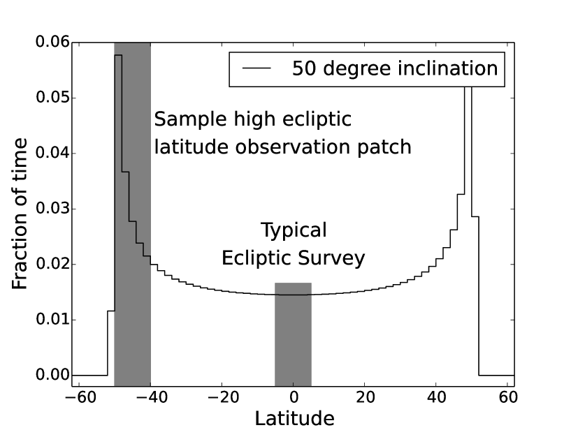
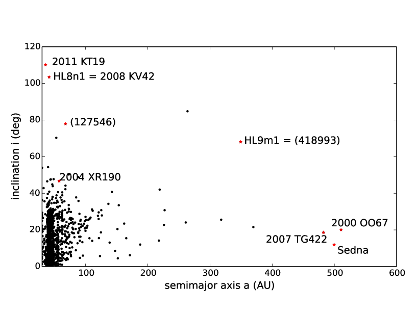
Kuiper Belt objects with large inclinations spend the majority of their time at high ecliptic latitudes (Fig. 1) and are poorly represented in the ecliptic surveys (including the main component of CFEPS). Even more dramatically, it has become clear that the size distribution of the high inclination component is flatter (number of objects increases slower when size decreases) than the ecliptic component (P1; Levison & Stern, 2001; Bernstein et al., 2004; Fraser et al., 2014). So deeper surveys concentrating on the ecliptic will be increasingly dominated by low inclination objects.
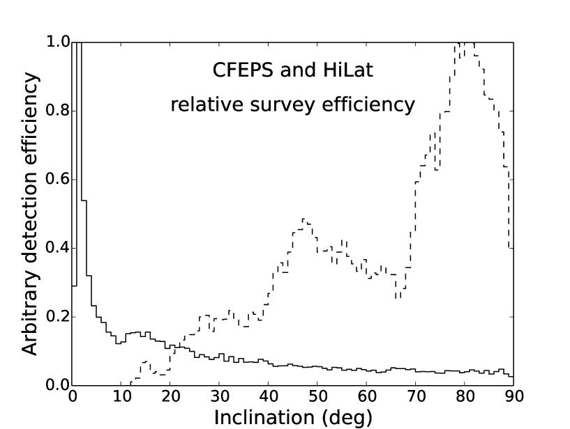
The situation at the end of 2006 was that a large fraction of the sky within a few degrees of the ecliptic had been covered by a few large surveys, with magnitude limits in the range of =20–23. Being insensitive to high inclination objects (Fig. 2), ecliptic surveys have poor sensitivity to the width of the hot population. Thanks to two deep blocks of 11 deg2 (one at 10∘ and another at 20∘ ecliptic latitude) the CFEPS efficiency decreases less than most other ecliptic surveys towards higher ecliptic latitudes. Still, although CFEPS preferes a hot population inclination width of 16∘, it could not reject a width of 25∘. Actually what limits the value of is the relative decrease of the number of low and intermediate inclination objects when increasing . Using the converted Palomar Schmidt, Trujillo & Brown (2003) had examined the majority of the northern sky to a depth of (limit for median observing conditions), discovering several of the largest known objects; several of these large-inclination objects (like Eris) were close to the depth and motion limits of that survey due to their great distances. The ESSENCE Supernova Survey (Becker et al., 2008) announced the detection of 14 TNOs found in images covering 11 deg2 to in the ecliptic latitude range -21∘ to -5∘; this work also showed that once outside of the ecliptic core, the sky density is consistent with even a uniform distribution in latitude. Such a distribution would not be rejected by any characterized surveys known at the time. We decided to perform a deep survey to magnitude 23.5–24.0 at high () ecliptic latitudes, called HiLat, to probe the hot component of the Kuiper Belt at sizes smaller than achieved by the Palomar wide area survey (Trujillo & Brown, 2003) and SDSS. Although HiLat is insensitive to objects with inclinations below 10∘ ecliptic latitude (Fig. 2), it complements existing surveys because its design makes it very sensitive to objects having inclinations beyond 20∘–30∘ (Fig. 2).
This manuscript describes the observations carried out during the six years of the project and provides our complete catalog (the HiLat release) of off-ecliptic detections and characterizations along with fully linked high-quality orbits. In summary, the ‘products’ of the HiLat survey consist of four items:
-
1.
A list of detected HiLat TNOs, associated with the sky location of discovery,
-
2.
a characterization of each survey discovery observation (detection efficiency as a function of magnitude, motin on sky; rate range searched; pointing of observations; etc.),
-
3.
a Survey Simulator that takes a proposed Kuiper Belt model, exposes it to the known detection biases of the HiLat blocks and produces simulated detections to be compared with the real detections, and
-
4.
the updated CFEPS model populations accounting for the HiLat detections.
2 Observations and Initial Reductions
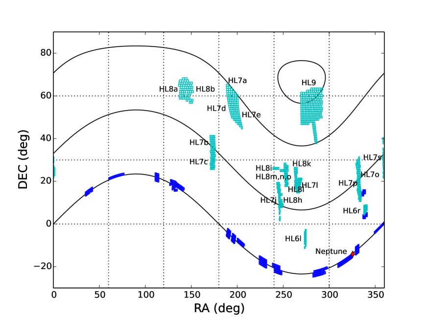
The discovery component of the HiLat project imaged 700 square degrees of sky, all of which was at ecliptic latitude larger than 12∘, extending almost to the North ecliptic pole (85∘, Fig. 3). Discovery observations, comprising a triplet of images 1 hour apart each on the date listed in Table 1, and a nailing observation, a single image acquired a few nights away from the discovery triplet, were all acquired using the Canada-France-Hawaii Telescope (CFHT) MegaPrime camera which delivered discovery image quality (FWHM) of 0.7–0.9 arc-seconds in queue-mode operations. The observations occured in blocks of 11 to 32 contiguous fields, cycling three times between the fields. The number of fields observed in a series was chosen such as to have 1 hour between two consecutive observations of the same field. When a block was too large to be observed within one night, it was split into two sub-blocks observed during close-by nights, with similar observing conditions. All discovery imaging data is publicly available from the Canadian Astronomy Data Centre (CADC444http://www.cadc.hia.nrc.gc.ca).
| Block | RA | Dec | Area | Fill | Detections | Ecl. lat. | Discovery | limit | Detection limits | |||
|---|---|---|---|---|---|---|---|---|---|---|---|---|
| HRS | deg | deg2 | Factor | D | T | range (deg) | date | filter | rate (“/h) | direction (deg) | ||
| HL6l | 18:16 | -06:49 | 15 | 0.80 | 0 | 0 | 11:50–20:50 | 2006-06-23 | r.MP9601 | 22.37 | 0.5 to 6.1 | -17.8 to 16.4 |
| HL6r | 22:37 | +07:04 | 16 | 0.80 | 7 | 6 | 12:20–16:40 | 2006-09-18 | r.MP9601 | 23.89 | 0.5 to 6.1 | -43.6 to -8.2 |
| HL7a | 13:06 | +55:00 | 32 | 0.90 | 0 | 0 | 49:40–60:00 | 2007-03-18 | r.MP9601 | 23.58 | 0.5 to 5.7 | 6.6 to 47.8 |
| HL7b | 11:33 | +37:30 | 32 | 0.88 | 0 | 0 | 27:00–35:40 | 2007-03-23 | r.MP9601 | 22.89 | 0.5 to 5.4 | -10.0 to 33.8 |
| HL7c | 11:33 | +29:30 | 32 | 0.89 | 4 | 4 | 19:50–28:40 | 2007-03-21 | r.MP9601 | 23.72 | 0.5 to 5.8 | -3.1 to 36.3 |
| HL7d | 12:49 | +57:00 | 32 | 0.84 | 0 | 0 | 49:30–59:50 | 2007-04-09 | r.MP9601 | 23.28 | 0.5 to 4.6 | -25.7 to 26.9 |
| HL7e | 13:23 | +52:58 | 32 | 0.87 | 0 | 0 | 49:40–60:10 | 2007-04-22 | r.MP9601 | 23.47 | 0.5 to 4.7 | -25.2 to 27.0 |
| HL7j | 16:22 | +12:53 | 32 | 0.90 | 5 | 5 | 22:50–40:20 | 2007-06-12 | r.MP9601 | 23.49 | 0.5 to 5.6 | -22.0 to 19.8 |
| HL7l | 17:47 | +18:03 | 27 | 0.90 | 0 | 0 | 37:50–45:00 | 2007-06-12 | r.MP9601 | 23.35 | 0.5 to 6.2 | -10.1 to 22.1 |
| HL7o | 22:12 | +22:02 | 32 | 0.90 | 0 | 0 | 20:30–39:40 | 2007-08-20 | r.MP9601 | 22.74 | 0.5 to 6.3 | -28.0 to 1.2 |
| HL7p | 22:06 | +19:23 | 32 | 0.84 | 4 | 4 | 19:40–39:10 | 2007-09-06 | r.MP9601 | 23.85 | 0.5 to 6.2 | -41.3 to -7.3 |
| HL7s | 23:59 | +27:54 | 31 | 0.98 | 0 | 0 | 19:30–37:00 | 2007-09-19 | r.MP9601 | 23.38 | 0.5 to 6.3 | -35.3 to -3.9 |
| HL8a | 09:24 | +63:30 | 30 | 0.90 | 1 | 1 | 40:00–50:20 | 2008-01-08 | r.MP9601 | 23.76 | 0.6 to 6.6 | 22.1 to 50.1 |
| HL8b | 09:52 | +61:60 | 25 | 0.90 | 0 | 0 | 40:30–49:50 | 2008-01-09 | r.MP9601 | 23.24 | 0.6 to 6.6 | 26.0 to 54.0 |
| HL8h | 16:32 | +09:58 | 11 | 0.88 | 0 | 0 | 29:10–35:50 | 2008-05-05 | r.MP9601 | 23.91 | 0.5 to 6.2 | 5.4 to 35.8 |
| HL8i | 16:21 | +25:33 | 11 | 0.90 | 0 | 0 | 44:40–47:30 | 2008-05-09 | r.MP9601 | 24.31 | 0.5 to 6.3 | 8.1 to 37.5 |
| HL8k | 17:35 | +24:25 | 12 | 0.90 | 1 | 1 | 44:50–49:50 | 2008-05-11 | r.MP9601 | 24.63 | 0.5 to 6.4 | 16.4 to 41.0 |
| HL8l | 17:36 | +19:15 | 13 | 0.90 | 0 | 0 | 39:40–45:50 | 2008-05-13 | r.MP9601 | 24.15 | 0.5 to 6.3 | 13.0 to 38.8 |
| HL8m | 16:58 | +23:15 | 12 | 0.90 | 0 | 0 | 39:50–49:50 | 2008-05-30 | r.MP9601 | 24.26 | 0.5 to 6.1 | -7.9 to 26.1 |
| HL8n | 16:53 | +22:33 | 11 | 0.89 | 1 | 1 | 39:40–50:30 | 2008-05-31 | r.MP9601 | 24.80 | 0.5 to 6.1 | -9.1 to 25.5 |
| HL8o | 16:48 | +23:00 | 12 | 0.90 | 0 | 0 | 39:30–50:20 | 2008-06-07 | r.MP9601 | 24.26 | 0.5 to 5.8 | -17.7 to 21.1 |
| HL9 | 18:45 | +55:08 | 219 | 0.92 | 1 | 1 | 59:30–85:20 | 2009-06-16 | r.MP9601 | 24.28 | 0.5 to 20.0 | -20.0 to 90.0 |
| Grand Total | 701 | 24 | 21 | |||||||||
Note. — RA/Dec is the approximate center of the field. Fill Factor is the fraction of the rectangle Area covered by the mosaic and useful for TNO searching. D is the number of TNOs detected in the block, T is the number of them that have been tracked to dynamical classification. Only one HL6r detection with apparent magnitude beyond the characterization limit, was not tracked to a high-quality orbit. The limiting magnitude of the survey, , is in the SDSS photometric system and corresponding to a 40% efficiency of detection. Detection limits give the limits on the sky motion in rate (“/hr) and direction (“zero degrees” is due West, and positive to the North).
The HiLat designation of a block was: a leading ‘HL’ followed by the year of observations (6 to 9) and then a letter representing the two week period of the year in which the search observations were acquired (example: HL7j occured in the second half of May 2007), similar to CFEPS naming scheme. Discovery observations occurred between June 2006 and June 2008 for the coverage below 60∘ ecliptic latitude, followed by observations between 60∘ and 85∘ ecliptic latitude from May to July 2009. This last part of the survey is simply named HL9 as it was acquired as 22 contiguous blocks over this time span.
The discovery fields were chosen in order to maximize our sensitivity to the latitude distribution of the Kuiper Belt, in particular the high inclination TNOs. Observing at high ecliptic latitude ensured that we observed only high-inclination TNOs, and greatly decreased the pressure for follow-up observations, as the number of TNOs per unit area drops sharply away from the ecliptic. The ecliptic longitudes were chosen to avoid the galactic plane, and maximize our chances to get discovery and tracking observations (due to typical weather at time of opposition for the discovery field, observing request pressure on the telescope). Each of the discovery blocks was searched for TNOs using our Moving Object Pipeline (MOP; see Petit et al., 2004). Table 1 provides a summary of the survey fields, imaging circumstances and detection thresholds. Subsequent tracking, over the next 2 or more oppositions, occurred at a variety of facilities, including CFHT, summarized in Table 2. The field sequencing and follow-up strategy of this survey are similar to those of CFEPS (Allen et al., 2006; Kavelaars et al., 2009; Petit et al., 2011). Our discovery and tracking observations were made using short exposures designed to maximize the efficiency of detection and tracking of the TNOs in the field. These observations do not provide the high-precision flux measurements necessary for possible taxonomic classification based on broadband colours of TNOs and we do not comment here on this aspect of the HiLat sample.
| UT Date | Telescope | Obs. | UT Date | Telescope | Obs. | ||
|---|---|---|---|---|---|---|---|
| 2006 Nov 22 | WIYN 3.5-m | 8 | 2008 Aug 31 | CFHT 3.5-m | 6 | ||
| 2007 Apr 13 | CFHT 3.5-m | 6 | 2008 Oct 22 | WIYN 3.5-m | 9 | ||
| 2007 May 14 | Hale 5-m | 13 | 2008 Dec 15 | Hale 5-m | 13 | ||
| 2007 May 14 | KPNO 2.1-m | 7 | 2008 Dec 20 | WIYN 3.5-m | 17 | ||
| 2007 Jul 26 | CFHT 3.5-m | 3 | 2009 Jan 26 | CFHT 3.5-m | 7 | ||
| 2007 Sep 10 | WIYN 3.5-m | 8 | 2009 Mar 25 | Subaru 8.2-m | 2 | ||
| 2007 Sep 13 | CFHT 3.5-m | 20 | 2009 Apr 22 | Subaru 8.2-m | 5 | ||
| 2007 Sep 15 | Hale 5-m | 25 | 2009 Jun 19 | WIYN 3.5-m | 30 | ||
| 2007 Oct 07 | CFHT 3.5-m | 6 | 2009 Jul 18 | CFHT 3.5-m | 5 | ||
| 2007 Nov 08 | WIYN 3.5-m | 17 | 2009 Jul 23 | Hale 5-m | 31 | ||
| 2008 Mar 04 | CFHT 3.5-m | 12 | 2009 Aug 17 | Hale 5-m | 6 | ||
| 2008 Mar 08 | CFHT 3.5-m | 3 | 2009 Aug 18 | CFHT 3.5-m | 6 | ||
| 2008 Apr 04 | CFHT 3.5-m | 10 | 2009 Sep 12 | CFHT 3.5-m | 4 | ||
| 2008 May 02 | WIYN 3.5-m | 21 | 2009 Sep 13 | CFHT 3.5-m | 27 | ||
| 2008 May 05 | CFHT 3.5-m | 21 | 2009 Oct 12 | CFHT 3.5-m | 8 | ||
| 2008 May 28 | CFHT 3.5-m | 14 | 2009 Nov 15 | CFHT 3.5-m | 4 | ||
| 2008 Jun 01 | CFHT 3.5-m | 3 | 2010 Jan 20 | CFHT 3.5-m | 3 | ||
| 2008 Jun 07 | CTIO 4-m | 20 | 2010 Mar 19 | Hale 5-m | 12 | ||
| 2008 Jun 22 | MMT 6.5-m | 4 | 2011 May 02 | Magellan 6.5-m | 8 | ||
| 2008 Jul 07 | Gemini South 8.1-m | 5 | 2013 Feb 06(a) | Gemini North 8.1-m | 42 | ||
| 2008 Aug 05 | CFHT 3.5-m | 24 | 2013 Jul 05 | NOT 2.5-m | 13 | ||
| 2008 Aug 30 | CFHT 3.5-m | 52 | 2013 AUg 05(a) | Gemini North 8.1-m | 32 |
Note. — All observations not part of the HiLat discovery survey are reported here. UT Date is the start of the observing run; Obs. is the number of astrometric measures reported from the observing run. Runs with low numbers of astrometric measures were either wiped out by poor weather, or not meant for HiLat object follow-up originally. This is the date of the first observation; targets were observed twice a month throughout the semester.
3 Sample Characterization
As is now the norm (Trujillo & Jewitt, 1998; Jewitt et al., 1998; Gladman et al., 1998; Trujillo et al., 2000; Gladman et al., 2001; Petit et al., 2006; Kavelaars et al., 2009; Petit et al., 2011), we characterized the magnitude-dependent detection probability of each discovery block by inserting artificial sources in the images. We performed differential aperture photometry for each of our detected objects observed on photometric nights. Our photometry is reported in the Sloan system (Fukugita et al., 1996) with the calibrations contained in the header of each image as provided by the ELIXIR processing software (Magnier & Cuillandre, 2004). It can be found in Tables 3 and 4. All HiLat discovery observations that detected TNOs were acquired in photometric conditions in a relatively narrow range of seeing conditions due to queue-mode acquisition.
Those real objects in each block that have a magnitude brighter than that block’s 40% detection probability are considered to be part of the HiLat characterized sample. Because detection efficiencies below 40% determined by human operators and our software diverge (Petit et al., 2004), and since characterization is critical to our goals, we are unable to utilize the sample faint-ward of the measured 40% detection efficiency level for quantitative analysis (although we report these discoveries, the majority of which were tracked to precise orbits). The characterized HiLat sample consists of 21 objects of the 24 discovered (Table 3). The magnitude distribution of objects detected brighter than our cutoff is consistent with the shape of the TNO luminosity function (Petit et al., 2008) and the typical decay in detection efficiency due to gradually increasing stellar confusion and the rapid fall-off at the SNR limit.
| DESIGNATIONS | Comment | ||||||||
|---|---|---|---|---|---|---|---|---|---|
| CFEPS | MPC | (AU) | (∘) | (AU) | |||||
| Resonant Objects | |||||||||
| HL6r3 | 2006 SG415 | 47.931(6) | 0.2915(1) | 31.376(0) | 35.009 | 23.27 | 0.03 | 7.75 | 2:1 |
| HL7j3 | 2007 LG38 | 55.45(2) | 0.4340(3) | 32.579(0) | 32.219 | 22.93 | 0.09 | 7.68 | 5:2 |
| HL7c1 | 2007 FN51 | 87.49(3) | 0.6188(2) | 23.237(0) | 39.100 | 23.20 | 0.06 | 7.17 | 5:1 I |
| HL7j4 | 2007 LF38 | 87.57(3) | 0.5552(2) | 35.825(0) | 48.432 | 22.53 | 0.09 | 5.54 | 5:1 I |
| Inner Classical Belt | |||||||||
| HL7p1 | 2007 RY326 | 38.817(9) | 0.06776(9) | 25.479(0) | 37.952 | 23.20 | 0.12 | 7.30 | |
| Main Classical Belt | |||||||||
| HL6r1 | 2007 RL314 | 40.386(8) | 0.0386(4) | 21.057(1) | 40.771 | 22.97 | 0.07 | 6.79 | |
| HL6r5 | 2006 SE415 | 42.599(8) | 0.027(1) | 18.517(1) | 42.266 | 23.73 | 0.12 | 7.40 | |
| HL6r6 | 2006 SF415 | 43.20(2) | 0.077(1) | 15.712(0) | 40.713 | 23.87 | 0.09 | 7.70 | |
| HL7c2 | 2007 FM51 | 45.53(1) | 0.159(1) | 29.221(1) | 42.561 | 23.00 | 0.15 | 6.59 | |
| HL7p2 | 2007 RW326 | 45.92(1) | 0.2355(2) | 20.500(0) | 35.127 | 23.70 | 0.10 | 8.16 | I (17:9) |
| HL7p3 | 2007 RX326 | 46.096(7) | 0.1565(3) | 25.029(0) | 39.343 | 23.30 | 0.30 | 7.25 | |
| Detached/Outer Classical Belt | |||||||||
| HL6r2 | 2006 SH415 | 49.759(9) | 0.2539(3) | 25.048(0) | 38.189 | 23.60 | 0.06 | 7.71 | |
| HL7c3 | 2007 FO51 | 50.37(3) | 0.2873(6) | 27.946(0) | 37.560 | 22.87 | 0.19 | 6.99 | I (13:6) |
| HL7j5 | 2007 LE38 | 54.05(1) | 0.2267(1) | 35.966(1) | 41.800 | 23.27 | 0.07 | 6.93 | |
| HL6r4 | 2007 RM314 | 70.81(2) | 0.4846(2) | 20.884(0) | 42.622 | 22.70 | 0.17 | 6.33 | I (18:5) |
| HL7j1 | 2007 LJ38 | 72.37(3) | 0.4698(3) | 31.540(0) | 38.848 | 23.07 | 0.19 | 7.03 | I (15:4) |
| HL8k1 | 2008 JO41 | 87.35(2) | 0.5431(1) | 48.815(0) | 44.453 | 24.57 | 0.12 | 7.91 | |
| Scattering Disk | |||||||||
| HL8a1 | 2008 AU138 | 32.392(3) | 0.3745(2) | 42.826(1) | 44.518 | 22.93 | 0.23 | 6.29 | |
| HL8n1 | 2008 KV42 | 41.532(4) | 0.49138(7) | 103.447(0) | 31.849 | 23.73 | 0.03 | 8.52 | |
| HL7j2 | 2007 LH38 | 133.93(4) | 0.72523(8) | 34.197(0) | 37.376 | 23.37 | 0.03 | 7.50 | I (19:2) |
| HL9m1 | 2009 MS9 | 348.9(2) | 0.96847(1) | 68.016(0) | 12.872 | 21.13 | 0.09 | 9.57 | |
Note. — : semimajor-axis (AU); : eccentricity; : inclination (degrees); : distance to the Sun at discovery time (AU); : apparent magnitude of the object in MegaPrime filter; : uncertainty on the magnitude in that filter; is the absolute magnitude in r band, given the distance at discovery; In Comment column, M:N: object in the M:N resonance; I: indicates that the orbit classification is insecure (see Gladman et al. (2008) for an explanation of the exact meaning); (M:N): the insecure object may be in the M:N resonance. For the orbital elements the number in “()” gives the uncertainty on the last digit.
| DESIGNATIONS | Comment | ||||||||
|---|---|---|---|---|---|---|---|---|---|
| CFEPS | MPC | AU | ∘ | AU | |||||
| Resonant Objects | |||||||||
| uHL7c4 | 2007 FP51 | 44.760(6) | 0.2017(1) | 25.606(0) | 36.688 | 23.80 | 0.20 | 8.02 | 20:11 I |
| Detached Classical Belt | |||||||||
| uHL7p4 | 2007 RZ326 | 52.676(8) | 0.3465(1) | 37.268(0) | 38.300 | 23.93 | 0.09 | 7.98 | |
| Non classified objects | |||||||||
| uHL6r7 | 2006 SN415 | — | — | — | 38(7) | 24.50 | 0.25 | 8.65 | |
Note. — Same as Table 3 for non characterized objects.
4 Tracking
For typical (i.e., low ecliptic latitude) surveys to depth 23.5–24, the observing load of tracking observations to secure the objects and determine their orbits represents many times the time spent for discovery. In such a case, a 700 square degree survey with fully tracked objects would be prohibitive. However, because HiLat covers very high ecliptic latitudes, the number of object per square degree at our limiting magnitude goes down dramatically beyond 30–35∘ and we detected only 24 objects (21 characterized). Hence the tracking observing load was much lower than for an ecliptic survey and
All of the 21 characterized and 2 of the 3 non-characterized objects were followed for at least 3 oppositions. Objects that still had uncertain dynamical classifications were then followed up to 7 oppositions, mostly for resonant or near-resonant objects. The global release of the complete observing record for all HiLat objects is available from the MPC (Petit et al., 2015) and the entire astrometric data for the HiLat objects can be found on the Besançon TNO database555http://tnodb.obs-besancon.fr/. The correspondence between HiLat internal designations and MPC designations can be determined using Tables 3 and 4 or from the Besançon TNO database. All characterized and tracked objects are prefixed by HL and are used with the survey simulator for our modelling below.
The tracking observations provide sufficient information to allow reliable orbits to be determined such that unambiguous dynamical classification can be achieved in the majority of cases. Orbital elements are computed using the Bernstein & Khushalani (2000) ‘orbfit’ code. Ephemerides errors for the coming year are as small as a few tenths of an arcsecond for several objects, others have uncertainties up to of order 10 arcseconds. Our protocol was to pursue tracking observations until the semimajor axis uncertainty was %; in Tables 3 and 4, orbital elements are shown to the precision with which they are known, with typical fractional accuracies on the order of a few . In the cases of resonant objects even this precision may not be enough to precisely determine the amplitude of the resonant argument, or even securely classify them as resonant. Thanks to our intensive tracking effort, dynamical classification is possible for 100% of the characterized sample.
4.1 Orbit classification
We follow the dynamical classification scheme of Gladman et al. (2008), which was also used to determine the classification of the CFEPS sample. In this scheme, the Kuiper Belt is divided into three broad orbital classes based on orbital elements and dynamical behavior. We first check if the object is resonant (currently in MMR with Neptune or Uranus), then see if it is currently scattering (practically defined as a variation of semimajor axis of more than 1.5 AU in a forward time integration over 10 Myr). If not, it is a classical or detached object: Inner classical if semimajor axis is interior to the MMR 3:2 with Neptune; main classical if semimajor axis between the 3:2 and 2:1 MMR; outer classical if semimajor axis beyond the 2:1 MMR and ; detached if semimajor axis beyond the 2:1 MMR and ).
Using this classification procedure, 7 of our 21 characterized objects remain insecure, as defined in Gladman et al. (2008), due to their proximity to a (high-order) resonance border where the remaining astrometric uncertainty makes it unclear if the object is actually resonant. We list these “insecure” objects in the category shown by the majority of the clones (Gladman et al., 2008) and give the nearby resonance in the comment column. Table 3 gives the classification of all characterized objects. None of these objects had archival observations before our discovery. Table 4 gives the classification of the tracked objects below the 40% detection efficiency threshold, hence deemed un-characterized and not used in our Survey Simulator comparisons.
The apparent motion of TNOs in our opposition discovery fields is approximately (”/hr) (147 AU)/, where is the heliocentric distance in AU. With a typical seeing of 0.7–0.9 arcsecond and a time base of 70–90 minutes between first and third frames, we were sensitive to objects as distant as 125 AU, provided they are brighter than our magnitude limit. Despite this sensitivity to large distances, the most distant object discovered in HiLat lies at 48.4 AU from the Sun (HL7j4, an insecure resonant object in the 5:1 MMR with Neptune (Pike et al., 2015)).
5 Results
CFEPS data presented in P1 were modelled independently for the inner, main, outer/detached classical, the scattering and various resonant populations by P1 and Gladman et al. (2012). The model for the main classical belt is refered as the L7 model hereafter. According to P1, the cold component may very well exist only in the main classical belt. The hot component, on the contrary, permeates the whole belt, from the inner classical, to the main classical, to the outer/detached belt and all the resonances. The cold component was well constrained by the Ecliptic component of the survey.
HiLat was designed to have maximum sensitivity to high-inclination objects (Fig. 2), and thus places strong constraints on the distribution of high-inclination objects, i.e., the hot population. The goal is thus to improve the L7 model.
5.1 Main Classical belt and L7 model
Our aim is to create a model that is compatible with both the CFEPS and HiLat detections. We are able to account for HiLat detections by slightly changing some parameters of the L7 orbital model, affecting only regions of phase space not well constrainted by CFEPS detections. Here we concentrate on the model for the main classical belt, because this dynamical class alone constitutes nearly a third of the full HiLat sample. With the parameterization of L7 model, HiLat is sensitive almost exclusively to the hot component. Hence this is the part of the model that will be modified in the following. However, in what follows, we always run the full L7 model, including all components: kernel, stirred and hot components.
5.1.1 Orbital model
To estimate the quality of a model, we compare the survey detected sample to the sample returned by passing our intrinsic model through a survey simulator (see Jones et al., 2006, for details). Acceptance of a model is based on the Anderson-Darling statistic for each of , , , [perihelion distance], and and its level of significance (probability of the null hypothesis [the simulated and the observed samples are drawn from the same underlying distribution] being correct), determined using a bootstrap method (Press et al., 1992). gives the rejectability of that hypothesis. As for CFEPS, we reject a model when the rejectability exceeds 95%. We determine the rejectability on the maximum of all 6 indicators we consider. When creating the L7 model, P1 split the phase space into sub-regions (see Appendix A of P1) to help separate the hot and cold components and account for the kernel and stirred components. HiLat detects almost exclusively the hot component, and the sample size is small, thus we determine the significance examining the full orbital phase space occupied by the main-belt.
Using the improved survey simulator (see Bannister et al. (2016a) for a description of the improvements) against the CFEPS detections, the L7 model for the main classical belt retains the same level of significance (20%) as with the previous survey simulator.
To combine the CFEPS and HiLat sample we must make a colour correction. CFEPS was run mostly with the filter, except for 1 block with the filter, and the pre-survey block with the R filter. HiLat was run entirely with the filter. The improved Survey Simulator correctly handles surveys observed in different filters, and accepts as input the colours of each object. Here, for compatibility with previous works, we assume and R (this assumption agrees with more recent results from OSSOS, the Outer Solar System Origin Survey; Bannister et al., 2016a).
When the biased L7 model is tested agaijnst the HiLat detections, the and distributions of the hot component are rejectable at %. An important feature of the L7 model for the main classical belt is the distribution of the hot component (see Appendix A of P1), which is essentially uniform between two limits, with rapid roll-over at both ends, with a width of 0.5 AU. The upper limit is poorly constrained by CFEPS. To account for HiLat detections, we moved the upper roll-over of the hot-component distribution from 40 to 41 AU, still with a width of 0.5 AU. Because HiLat did not detect any main classical belt object with AU, we must impose a sharp cut-off on top of the -dependent lower-limit of the hot-component distribution. The new parameterization is described in Appendix A. Using this slight tuning of the L7 model continues to provide an acceptable match to the CFEPS detected sample, when considered independent of the HiLat sample. Extending the -distribution of the L7 model somewhat allows compatibility with the HiLat -distribution.
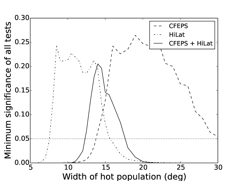
The -distribution of the HiLat main classical belt detected sample is incompatible with the hot component of the L7 model. The CFEPS detected sample strongly rejects a hot population with a narrow inclination width because that model does not yield the correct ratio between low inclination and high inclination as compared to the detections in the CFEPS sample. The CFEPS sample rejects much larger inclination distributions (; see Fig. 4, dashed line) only because of the relative lack of low inclination objects in these distributions. The HiLat detected sample, on the contrary, rejects any model with too wide an inclination distribution because this survey is very sensitive to the high inclination orbits. Even the inclination width preferred by CFEPS has a long tail containing too many objects with which would have been detected by HiLat. But being completely insensitive to low inclination orbits (HiLat cannot detect any of them), it can accept any values of as long at they allow enough objects up to . Thus HiLat is consistent with all values of from 7.5∘ to 15.5∘ (Fig. 4, dash-dotted line). Together, the two surveys combine high CFEPS sensitivity at low inclinations and HiLat’s improved sensitivity at high inclinations. The result is shown in Fig. 4. Because our model rejection threshold is set at 5% significance, this analysis indicates that an acceptable value for each of CFEPS and HiLat separately and for their combination, is an inclination width in the range 14∘–15.5∘, where all three curves exceed the threshold.
Separately, CFEPS and HiLat favor different values for the width and only marginally agree at the intersection (see Fig. 4). There is tension between the models allowed by the two data sets. This raises doubts on the parameterization used here. Gulbis et al. (2010) introduced an inclination distribution given by times a Gaussian of width , centered on a value greater than 0∘ to fit what they called the Scattered population (Appendix A). Pike et al. (2015) did the same to study the 5:1 MMR population. P1 mentioned the possibility to use a similar functional form to represent the Classical belt hot population inclination distribution, but concluded that the fit was good enough with the usual distribution and that the data did not demand the increased complexity of the extra parameter. Applying this functional form to the CFEPS, HiLat and CFEPS+HiLat sample also does not improve the level of significance enough to warrant the increased complexity of the extra parameter. So our preferred model retains the previous inclination distribution functional form, with a width . We note, however, that the functional form here, while useful for discussion, is not a good description of the physical distribution of high-inclination TNOs.
5.1.2 Population estimates
Population estimates are dependent on the orbital model used to describe each TNO component, which we are slightly modifying from P1. They also depend on the correct modelling of the survey operation and detection efficiency. As explained in Bannister et al. (2016a), the survey simulator has been improved to better represent the exact selection and rejection effects of objects based on measured magnitude rather than intrinsic magnitude. This has the potential of substantially affecting the population estimates due to the steep slopes of the absolute magnitude H distributions.
We follow the same procedure as in Kavelaars et al. (2009), Gladman et al. (2012), and P1. We run our model, generating simulated objects, passing them through the survey simulator until we have detected the same number of objects in the simulation as in the real survey(s). We record this number and repeat the procedure 500 times. This gives us the distribution of likely population size. Table 5, columns A, gives the population estimates, using our new model, to to compare with P1. Compared to P1, we use the new -distribution and an -distribution with width . Our CFEPS estimates are statistically undistinguishable from P1 estimates.
| Population | CFEPS | HiLat | CFEPS+HiLat | |||
|---|---|---|---|---|---|---|
| A | B | A | B | A | B | |
| hot | ||||||
| stirred | ||||||
| kernel | ||||||
Note. — Our model estimates are given for each sub-population within the Kuiper belt. The uncertainties reflect 95% confidence intervals for the model-dependent population estimate. Remember that the relative importance of each population will vary with the upper limit. The A columns correspond to a uniform colour = 0.7, while B columns have = 0.45 for the hot component and = 0.95 for the cold component.
Although the various population estimates for a given component have overlapping error bars, HiLat estimates population sizes at just a little over half those of CFEPS. This is also reflected in the larger than observed fraction of objects detected from HiLat when running our model through the combined CFEPS + HiLat survey simulator; 12% of the simulated detections are from HiLat, while they represent only 6% of the real sample. This larger fraction from HiLat means the model plus survey simulator are more efficient at detecting objects in HiLat survey, hence needing a smaller underlying population to reach the required number of detections. This may be due to our choice of color for TNOs, a necessary parameter when combining surveys done in different band passes.
Up to now we used the colour derived from CFEPS sample for all components. However, the cold belt objects are redder than the hot ones (Doressoundiram et al., 2002; Tegler et al., 2003). If the hot objects detected by HiLat are bluer than , then the number of objects brighter than needed to match the real detections is larger. According to Fraser (private communication, 2016), the cold component has a typical colour , while the hot component comprise mostly neutral objects with , and a small fraction of objects as red as the cold component. Table 5, columns B, gives the population estimates when using for the hot component and for the cold component. The three population estimates become more compatible with each other, and the fraction of simulated detections from HiLat in CFEPS+HiLat simulations becomes 7%, similar to the real detected fraction. This result provides (unsurprising) evidence for the already known different colours of the various components, which must be accounted for when combining detections in different filters.
5.2 Other populations
The HiLat characterized sample included six outer classical or detached objects, roughly half as many as were identified by CFEPS (P1 identified 13 non-scattering, non-resonant objects beyond 48 AU). P1 established that the outer-detached population can be interpreted as a smooth extention beyond the 2:1 MMR of the hot main classical belt. We confirm this result with CFEPS+HiLat detection. We note however that the HiLat sample alone allows inclination widths , possibly more excited than for the main classical belt. The combined CFEPS+HiLat sample allows an inclination width . This is in agreement with the outer-detached population being a smooth extension of the hot classical population. We estimate the population beyond 48 AU , very similar to P1 estimate.
The HiLat characterized sample contains 4 resonant objects. One is in the 2:1 MMR and another one in the 5:2 MMR with Neptune. These represent a small contribution to the known populations of these resonances from characterized surveys like CFEPS. HiLat made an important contribution to our understanding of the resonant population by discovering two objects in the 5:1 MMR (only 1 was known from CFEPS), and another very close to the 5:1 MMR, HL8k1 = 2008 JO41 at 87.356 AU; scientific interpretation of these discoveries have been reported in Pike et al. (2015).
5.3 Exotic objects: 2008 KV42 and (418993) 2009 MS9
Amongst its 21 characterized detections, HiLat discovered 2 extraordinary TNOs. Both are scattering objects. The first one was discovered on May 31st, 2008 in a field at moderate ecliptic latitude (). It is HL8n1 = 2008 KV42, the first known retrograde TNO. Details about this object and what it tells us about the origin and dynamical evolution of exotic scattering objects is developed in Gladman et al. (2009).
The second object is HL9m1 = (418993) 2009 MS9, discovered on the 26th of June 2009 at a distance of 12.9 AU from the Sun and an ecliptic latitude of 71∘. It has a large ( AU) and highly-inclined () orbit (Fig. 5), which is also highly eccentric (). Inbound at 13 AU at time of discovery, the pericenter of this extreme orbit was 11 AU in February 2013, so (418993) is transiting the range of heliocentric distances where comets have been observed to become active (Meech & Svoren, 2004). (418993) thus may be the first observable object that has been in deep cold storage at hundreds of AU for of order 5,000 years. Under the hypothesis that this is a comet from a distant source (either the inner Oort Cloud, or something else as yet unknown), it is also quite possible that (418993) has never been interior to Saturn’s orbit (unlikely to be true for the known Centaurs, which often have their perihelia altered as they interact with the giant planets).
A plausible scenario is that (418993) is a former Oort-cloud object that has had its orbit changed from nearly parabolic (1000 AU) to highly eccentric by an encounter with Saturn, Uranus, or Neptune. (418993) is currently only dynamically meta-stable on the order of 10 Myr, and may never have come inside the water-sublimation zone (heliocentric distances of 5–6 AU). Many comet nuclei have been studied after the development of a coma, but only after the comets have left the inner Solar System and are very dim (Lamy et al., 2004). MS9 had the advantages that, at time of discovery, it was bright ( 22), inbound, and had no obscuring coma. Assuming an albedo =0.04 (common for comet nuclei, Lamy et al., 2004, but on the lower end for TNOs), this object has a radius 20 km. Not only is (418993) unique dynamically, but if it had become an active comet, it would have been the largest comet nucleus in recent times, after Hale-Bopp (C/1995 O1; radius = 37 km; Lamy et al., 2004).
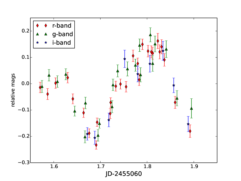
At its discovery distance of 13 AU, no coma has been detected in analysis of our deep August 2009 CFHT images, to a limit of 28 mag/arcsec2. Other shorter-period comets have been observed to start cometary activity as far out as 12–14 AU from the Sun (1P/Halley at 14 AU and 2060 Chiron at 12 AU; Meech & Svoren, 2004). We observed (418993) at the Palomar 5m in August 2009, and determined that it has a -mag lightcurve with a period of over either 6.5 (single peaked) or 13 hours (double peaked; Fig. 6). Studying a possible cometary activity on this object requires determining the rotational phase to remove this predictable brightness change. We obtained snapshot observations to monitor the cometary activity from Aug. 2010 to Feb 2011 but detected none. From 2012 until end of 2014, many observations of (418993) have been reported to MPC, around its perihelion passage, but none have reported detection of cometary activity.
6 Summary and discussion
The HiLat survey was designed to address one of the shortcomings of CFEPS, its lack of sensitivity to high-inclination objects. HiLat imaged about 700 sqr. deg. from 12∘ to 85∘ ecliptic latitude. The survey was performed at CFHT in the filter and achieved limiting magnitudes raging from for the shallowest field to for the deepest field. Being at high ecliptic latitude, the survey detected only 24 objects, of which 21 are brighter than the characterization limit. Thanks to the small number of objects and to our careful follow-up strategy, we tracked all characterized objects to precise orbit determination and orbital classification.
HiLat detected 6 objects from the hot main classical belt. We confirm the global parameterization of this component found by CFEPS. An important finding of CFEPS was that the -distribution of the hot classical component is essentially flat between 35 AU and 40 AU, with poor constraint on this upper limit. The HiLat sample requires us to move the upper limit to 41 AU. Including the HiLat sample and survey in the analysis, we decrease sightly the width of the inclination distribution of the hot component to .
The high sensitivity of HiLat survey to TNOs on highly-inclined orbits permits formal rejection at high confidence of ’wider’ orbital -distributions for the hot classical belt, and to a lesser extent the detached components. CFEPS survey already rejected ’narrower’ distributions. Having an -distribution with little contribution below about 10∘ and not extending much beyond 35∘–40∘ is difficult to achieve with a broad gaussian centered at distribution. It becomes increasingly clear that eq. (7) in Brown (2001) is not the approrpiate representation for this distribution and something different should be considered. The distribution proposed by Gulbis et al. (2010) is an interesting possibility. A new -distribution could have profound cosmogonic implications that would need to be investigated.
The exotic higher- objects like those found in HiLat (Fig. 5) do not fit into this picture; we will call these objects the ‘halo’ component. Due to our sensitivity to high inclinations, these do not represent the tail of the 14.5∘ gaussian. Instead, these objects may point to a new source that feeds large- TNOs into the planetary system (Gladman et al., 2009). This may simultaneously be the source of the Halley-Type comets (see Levison et al., 2006). Recently, Batygin & Brown (2016) pointed to (418993) as possible evidence that this source might be related to an undiscovered planet in the distant solar system ( au); producing objects like 2008 KV42 requires pulling objects from such a large- source down to such small semimajor axes and is exceedingly difficult due to the high encounter speeds with Neptune and Uranus (Gladman et al., 2009).
The OSSOS Survey (Bannister et al., 2016a, b) will allow a careful consideration of the details of the -distribution of the main hot component and the relative fraction of objects that must be in this halo population. The use of our characterized Hilat survey (coupled to CFEPS and OSSOS) permits powerful constraints to be placed on the distribution generated by any proposed model of where these extreme objects are coming from.
Appendix A Appendix A
We here detail the minor tuning to the L7 algorithm used to generate the hot population of the main classical belt, motivated by the HiLat sample’s greater sensitvity. The new algorithm becomes:
-
•
a perihelion distance distribution that is mostly uniform between 35 and 41 AU, with soft shoulders at both ends extending over 1 AU; the PDF is proportional to ; any object with 35 AU is rejected;
-
•
reject objects with (deg) to account for weaker long-term stability of low- orbits at low inclination.
The inclination distribution for the hot component remains , but with .
References
- Allen et al. (2006) Allen, R. L., Gladman, B., Kavelaars, J. J., Petit, J., Parker, J. W., & Nicholson, P. 2006, ApJ, 640, L83
- Bannister et al. (2016a) Bannister, M. T., Kavelaars, J. J., Petit, J.-M., Gladman, B. J., Gwyn, S. D. J., Chen, Y.-T., Volk, K., Alexandersen, M., Benecchi, S., Delsanti, A., Fraser, W., Granvik, M., Grundy, W. M., Guilbert-Lepoutre, A., Hestroffer, D., Ip, W.-H., Jakubik, M., Jones, L., Kaib, N., Lacerda, P., Lawler, S., Lehner, M. J., Lin, H. W., Lister, T., Lykawka, P. S., Monty, S., Marsset, M., Murray-Clay, R., Noll, K., Parker, A., Pike, R. E., Rousselot, P., Rusk, D., Schwamb, M. E., Shankman, C., Sicardy, B., Vernazza, P., & Wang, S.-Y. 2016a, AJ
- Bannister et al. (2016b) —. 2016b, In preparation
- Batygin & Brown (2016) Batygin, K. & Brown, M. E. 2016, AJ, 151, 22
- Becker et al. (2008) Becker, A. C., Arraki, K., Kaib, N. A., Wood-Vasey, W. M., Aguilera, C., Blackman, J. W., Blondin, S., Challis, P., Clocchiatti, A., Covarrubias, R., Damke, G., Davis, T. M., Filippenko, A. V., Foley, R. J., Garg, A., Garnavich, P. M., Hicken, M., Jha, S., Kirshner, R. P., Krisciunas, K., Leibundgut, B., Li, W., Matheson, T., Miceli, A., Miknaitis, G., Narayan, G., Pignata, G., Prieto, J. L., Rest, A., Riess, A. G., Salvo, M. E., Schmidt, B. P., Smith, R. C., Sollerman, J., Spyromilio, J., Stubbs, C. W., Suntzeff, N. B., Tonry, J. L., & Zenteno, A. 2008, ApJ, 682, L53
- Bernstein & Khushalani (2000) Bernstein, G. & Khushalani, B. 2000, AJ, 120, 3323
- Bernstein et al. (2004) Bernstein, G. M., Trilling, D. E., Allen, R. L., Brown, M. E., Holman, M., & Malhotra, R. 2004, AJ, 128, 1364
- Brasser et al. (2012) Brasser, R., Duncan, M. J., Levison, H. F., Schwamb, M. E., & Brown, M. E. 2012, Icarus, 217, 1
- Brown (2001) Brown, M. E. 2001, AJ, 121, 2804
- Brown et al. (2005) Brown, M. E., Trujillo, C. A., & Rabinowitz, D. L. 2005, ApJ, 635, L97
- Doressoundiram et al. (2002) Doressoundiram, A., Peixinho, N., de Bergh, C., Fornasier, S., Thébault, P., Barucci, M. A., & Veillet, C. 2002, AJ, 124, 2279
- Fraser & Brown (2012) Fraser, W. C. & Brown, M. E. 2012, ApJ, 749, 33
- Fraser et al. (2014) Fraser, W. C., Brown, M. E., Morbidelli, A., Parker, A., & Batygin, K. 2014, ApJ, 782, 100
- Fukugita et al. (1996) Fukugita, M., Ichikawa, T., Gunn, J. E., Doi, M., Shimasaku, K., & Schneider, D. P. 1996, AJ, 111, 1748
- Gladman & Chan (2006) Gladman, B. & Chan, C. 2006, ApJ, 643, L135
- Gladman et al. (2009) Gladman, B., Kavelaars, J., Petit, J., Ashby, M. L. N., Parker, J., Coffey, J., Jones, R. L., Rousselot, P., & Mousis, O. 2009, ApJ, 697, L91
- Gladman et al. (1998) Gladman, B., Kavelaars, J. J., Nicholson, P. D., Loredo, T. J., & Burns, J. A. 1998, AJ, 116, 2042
- Gladman et al. (2001) Gladman, B., Kavelaars, J. J., Petit, J.-M., Morbidelli, A., Holman, M. J., & Loredo, T. 2001, AJ, 122, 1051
- Gladman et al. (2012) Gladman, B., Lawler, S. M., Petit, J.-M., Kavelaars, J., Jones, R. L., Parker, J. W., Van Laerhoven, C., Nicholson, P., Rousselot, P., Bieryla, A., & Ashby, M. L. N. 2012, AJ, 144, 23
- Gladman et al. (2008) Gladman, B. J., Marsden, B. G., & van Laerhoven, C. 2008, in The Solar System Beyond Neptune, ed. A. Barucci, H. Boehnhardt, D. Cruikshank, & A. Morbidelli, LPI (Tucson: University of Arizona Press), 43–57
- Gulbis et al. (2010) Gulbis, A. A. S., Elliot, J. L., Adams, E. R., Benecchi, S. D., Buie, M. W., Trilling, D. E., & Wasserman, L. H. 2010, AJ, 140, 350
- Ida et al. (2000) Ida, S., Larwood, J., & Burkert, A. 2000, ApJ, 528, 351
- Jewitt et al. (1996) Jewitt, D., Luu, J., & Chen, J. 1996, AJ, 112, 1225
- Jewitt et al. (1998) Jewitt, D., Luu, J., & Trujillo, C. 1998, AJ, 115, 2125
- Jones et al. (2006) Jones, R. L., Gladman, B., Petit, J., Rousselot, P., Mousis, O., Kavelaars, J. J., Campo Bagatin, A., Bernabeu, G., Benavidez, P., Parker, J. W., Nicholson, P., Holman, M., Grav, T., Doressoundiram, A., Veillet, C., Scholl, H., & Mars, G. 2006, Icarus, 185, 508
- Jones et al. (2010) Jones, R. L., Parker, J. W., Bieryla, A., Marsden, B. G., Gladman, B., Kavelaars, J., & Petit, J. 2010, AJ, 139, 2249
- Kaib et al. (2011) Kaib, N. A., Roškar, R., & Quinn, T. 2011, Icarus, 215, 491
- Kavelaars et al. (2008) Kavelaars, J., Jones, L., Gladman, B., Parker, J. W., & Petit, J. The Orbital and Spatial Distribution of the Kuiper Belt, ed. Barucci, M. A., Boehnhardt, H., Cruikshank, D. P., & Morbidelli, A. , 59–69
- Kavelaars et al. (2009) Kavelaars, J. J., Jones, R. L., Gladman, B. J., Petit, J., Parker, J. W., Van Laerhoven, C., Nicholson, P., Rousselot, P., Scholl, H., Mousis, O., Marsden, B., Benavidez, P., Bieryla, A., Campo Bagatin, A., Doressoundiram, A., Margot, J. L., Murray, I., & Veillet, C. 2009, AJ, 137, 4917
- Kenyon & Bromley (2004) Kenyon, S. J. & Bromley, B. C. 2004, Nature, 432, 598
- Lamy et al. (2004) Lamy, P. L., Jorda, L., Toth, I., Weaver, H. A., Cruikshank, D., & Fernandez, Y. 2004, in COSPAR Meeting, Vol. 35, 35th COSPAR Scientific Assembly, ed. J.-P. Paillé, 1824
- Levison et al. (2010) Levison, H. F., Duncan, M. J., Brasser, R., & Kaufmann, D. E. 2010, Science, 329, 187
- Levison et al. (2006) Levison, H. F., Duncan, M. J., Dones, L., & Gladman, B. J. 2006, Icarus, 184, 619
- Levison et al. (2008) Levison, H. F., Morbidelli, A., Vanlaerhoven, C., Gomes, R., & Tsiganis, K. 2008, Icarus, 196, 258
- Levison & Stern (2001) Levison, H. F. & Stern, S. A. 2001, AJ, 121, 1730
- Magnier & Cuillandre (2004) Magnier, E. A. & Cuillandre, J.-C. 2004, PASP, 116, 449
- Meech & Svoren (2004) Meech, K. J. & Svoren, J. Using cometary activity to trace the physical and chemical evolution of cometary nuclei, ed. M. C. Festou, H. U. Keller, & H. A. Weaver, 317–335
- Millis et al. (2002) Millis, R. L., Buie, M. W., Wasserman, L. H., Elliot, J. L., Kern, S. D., & Wagner, R. M. 2002, AJ, 123, 2083
- Morbidelli & Levison (2004) Morbidelli, A. & Levison, H. F. 2004, AJ, 128, 2564
- Nesvorny (2015) Nesvorny, D. 2015, AJ, 150, 73
- Peixinho et al. (2015) Peixinho, N., Delsanti, A., & Doressoundiram, A. 2015, A&A, 577, A35
- Petit et al. (2004) Petit, J., Holman, M., Scholl, H., Kavelaars, J., & Gladman, B. 2004, MNRAS, 347, 471
- Petit et al. (2006) Petit, J., Holman, M. J., Gladman, B. J., Kavelaars, J. J., Scholl, H., & Loredo, T. J. 2006, MNRAS, 365, 429
- Petit et al. (2008) Petit, J., Kavelaars, J. J., Gladman, B., & Loredo, T. Size Distribution of Multikilometer Transneptunian Objects, ed. Barucci, M. A., Boehnhardt, H., Cruikshank, D. P., & Morbidelli, A. , 71–87
- Petit et al. (2015) Petit, J.-M., Allen, L., Gladman, B., Kavelaars, J., Nicholson, P., Jacobson, R., Brozovic, M., Lawler, S., Parker, J. W., & Williams, G. V. 2015, Minor Planet Electronic Circulars, 1
- Petit et al. (2011) Petit, J.-M., Kavelaars, J. J., Gladman, B. J., Jones, R. L., Parker, J. W., Van Laerhoven, C., Nicholson, P., Mars, G., Rousselot, P., Mousis, O., Marsden, B., Bieryla, A., Taylor, M., Ashby, M. L. N., Benavidez, P., Campo Bagatin, A., & Bernabeu, G. 2011, AJ, 142, 131
- Pike et al. (2015) Pike, R. E., Kavelaars, J. J., Petit, J. M., Gladman, B. J., Alexandersen, M., Volk, K., & Shankman, C. J. 2015, AJ, 149, 202
- Press et al. (1992) Press, W. H., Teukolsky, S. A., Vetterling, W. T., & Flannery, B. P. 1992, Numerical recipes in FORTRAN. The art of scientific computing
- Tegler et al. (2003) Tegler, S. C., Romanishin, W., & Consolmagno, G. J. 2003, ApJ, 599, L49
- Thommes et al. (1999) Thommes, E. W., Duncan, M. J., & Levison, H. F. 1999, Nature, 402, 635
- Trujillo & Jewitt (1998) Trujillo, C. & Jewitt, D. 1998, AJ, 115, 1680
- Trujillo & Brown (2003) Trujillo, C. A. & Brown, M. E. 2003, Earth Moon and Planets, 92, 99
- Trujillo et al. (2000) Trujillo, C. A., Jewitt, D. C., & Luu, J. X. 2000, ApJ, 529, L103
- Trujillo et al. (2001) —. 2001, AJ, 122, 457