Proximity effects in cold atom artificial graphene
Abstract
Cold atoms in an optical lattice with brick-wall geometry have been used to mimic graphene, a two-dimensional material with characteristic Dirac excitations. Here we propose to bring such artificial graphene into the proximity of a second atomic layer with a square lattice geometry. For non-interacting fermions, we find that such bilayer system undergoes a phase transition from a graphene-like semi-metal phase, characterized by a band structure with Dirac points, to a gapped band insulator phase. In the presence of attractive interactions between fermions with pseudospin-1/2 degree of freedom, a competition between semi-metal and superfluid behavior is found at the mean-field level. Using the quantum Monte Carlo method, we also investigate the case of strong repulsive interactions. In the Mott phase, each layer exhibits a different amount of long-range magnetic order. Upon coupling both layers, a valence-bond crystal is formed at a critical coupling strength. Finally, we discuss how these bilayer systems could be realized in existing cold atom experiments.
1 Introduction
The outstanding properties of graphene have boosted the interest in this two-dimensional, carbon-made material. Technology developments are linked mostly to its mechanical performances, large specific surface area and conductivity properties [1, 2]. On the fundamental side, the most intriguing properties emerge from the peculiar material’s band structure originating from the hexagonal geometry of the lattice, equivalent to two triangular Bravais lattices shifted relative to each other: each band is split into two separated ones. These bands touch each other at two distinct points within the first Brillouin zone, the so-called Dirac points. In the vicinity of the Dirac points, the dispersion is linear, and low-energy excitations behave like relativistic particles. Recently, there have been proposals to modify the band structure by bringing graphene on top of another graphene layer [3], or close to other substrates [4]. Furthermore, the emergence of additional Dirac points has been observed in graphene on hexagonal boron nitride [5]. The proximity of graphene to a normal two-dimensional electron gas was studied in Refs. [6, 7, 8].
A different approach to studying properties of the graphene band structure is the use of artificial graphene [9], that is, of systems that are designed to mimic graphene. Artificial graphene offers several control parameters allowing to tune the system. The variety of artificial graphene systems reaches from solid-state devices such as semiconductor structures with engineered nanopatterns [10, 11, 12], or molecules arranged on metal surfaces [13], to optical systems such as hexagonal photonic crystals [14, 15], microwave fields in metamaterial structures [16], or ultracold atoms in hexagonal optical lattices [17, 18]. The latter system offers a great deal of control, and several pioneering experiments have proven the versatility of cold atoms as quantum simulators during the past decade, cf. Ref. [19]. By engineering hexagonal optical lattices for bosons [17, 20, 21, 22, 23] and fermions [18, 24, 25, 26, 27], cold atom systems with graphene-like band structure have been realized in recent years. These experimental possibilities have also stimulated theoretical interest in atoms on hexagonal lattices [28, 29, 30, 31, 32, 33]. A particular feature of cold atoms in optical lattice is the tunability of the tunneling strengths. In the context of artificial graphene, this allows to smoothly introduce anisotropies, which can result into the merging of the Dirac points, and mass acquisition of the excitation [28, 29, 30, 18]. Furthermore, a gap at the Dirac points can be opened by introducing an energy offset between the two sublattices as studied experimentally in Refs. [18, 23, 25], or, more recently, by applying an artificial staggered magnetic field (realizing the celebrated Haldane model) [26].
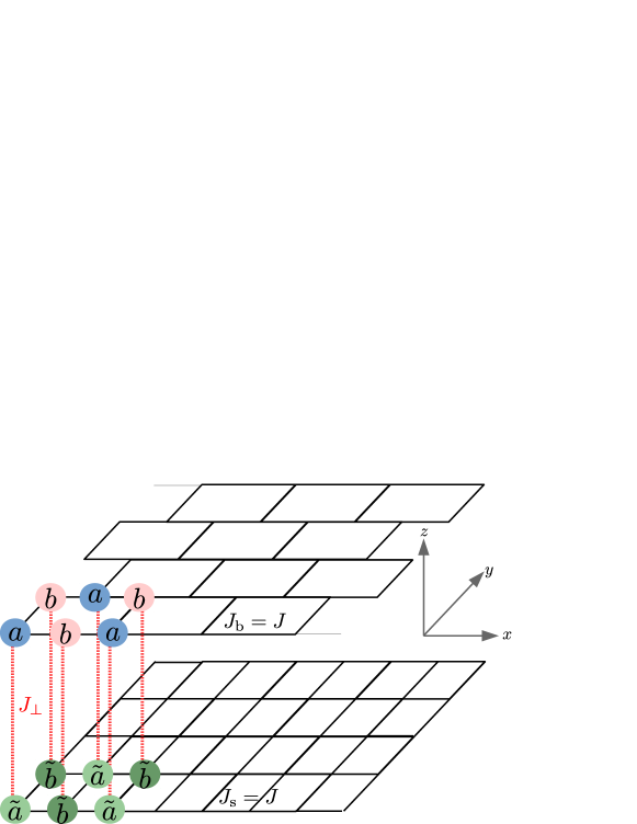
In the present paper we propose a different way for manipulating the band structure of artificial graphene of cold atoms in optical lattices. Motivated by the so-called “proximity effect” where different materials are placed together in order to engineer topological superconductors [34, 35, 36, 37], we consider a heterostructure of two layers with different dispersion. This scenario is closely related to the approaches recently used in real-graphene systems, where the proximity between graphene to other substrates is exploited both theoretically and experimentally. The proximity to hexagonal boron nitride has been studied in Refs. [4, 5]. A graphene layer close to a semi-conducting quantum well was considered in Refs. [6, 7, 8], studying the interplay of a two-dimensional electron gas with a layer of Dirac fermions. Such scenario is relevant also in the context of a recent experiment which implements an artificial-graphene layer on top of a semiconductor via electron-beam lithography [38, 12]. A somewhat similar setup is considered in the present paper. We theoretically study a bilayer structure, where one layer has a graphene-like band structure, while the other layer has square lattice geometry. As illustrated in Fig. 1(a), the “graphene” layer is realized by a brick-wall lattice, which regarding its band structure is equivalent to a hexagonal lattice. With this, the square layer perfectly matches the graphene lattice with respect to the atom positions. It differs, however, with respect to the coupling between the atoms, as in the brick-wall layer every second link along the -direction is missing. We then investigate the role of a coupling between the layers, for a non-interacting system in Sec. 3, for a system with weak attractive interactions in Sec. 4, and for a system with strong repulsive interactions in Sec. 5. We describe a scheme for realizing such system with cold atoms in optical lattices in Sec. 6.
The bilayer system here proposed manifests a rich set of physical phenomena. Our main findings are summarized as follows:
(i) In the non-interacting system, the number and position of Dirac points are controlled by the interlayer coupling. In the presence of interlayer coupling two additional Dirac points arise from intersections between brick-wall and square lattice dispersion. For strong coupling, the Dirac points stemming from the brick-wall dispersion merge and disappear. If prepared at half filling, the system then undergoes a transition from a semi-metal to a band insulator. At this transition, the lowest excitations are massless in one direction, but massive in the other direction.
(ii) For attractive interactions we find, within a mean-field approximation, a competition between superfluid and semi-metallic phases. In contrast to a single brick-wall layer, in the bilayer such competition also occurs at filling 1/4 and 3/4, due to the presence of additional Dirac points.
(iii) In the strongly repulsive system, for which the low-energy physics is described by an appropriate spin model, we have used the quantum Monte Carlo method in order to investigate the competition between long-range order within each layer, and dimerization of nearest-neighbors between the two layers. We have quantitatively determined the critical interlayer coupling at which a valence bond crystal is formed ().
2 System
As illustrated in Fig. 1, we consider a bilayer structure consisting of one square lattice on top of a brick-wall lattice. The brick-wall lattice mimics graphene, as it represents a deformed hexagonal lattice. Accordingly, we can divide it into two triangular sub-lattices, and , and the annihilation operators on these sub-lattices are denoted by and . Without coupling between the layers the unit cell of a square lattice contains only one atom. However, the presence of a finite coupling increases the unit cell to two atoms per layer, and we need to distinguish between the two sublattices also in the square layer. Accordingly, we denote the operators which annihilate particles in the square lattice by and . The index denotes the position of the annihilated particle within the -plane. With these definitions, and assuming isotropic couplings and in the square and the brick-wall lattice, respectively, the tight-binding Hamiltonian of the bilayer system reads
| (1) |
where is the interlayer coupling. The vectors and connect neighboring sites along the - and -direction. The sum over contains all nearest-neighbor pairs with in sublattice and in sublattice . The last sum, over , shall include all lattice points in the corresponding sublattice, i.e. it is restricted to sublattice for terms containing operators, and restricted to sublattice for terms containing operators.
Loading the lattice with spin-polarized fermions, no double-occupancies can occur, and interactions are avoided. In this scenario, further investigated in the next section, we can explore the band structure of the bilayer. Interesting many-body effects, considered in the subsequent sections, will occur when the lattice is loaded with fermionic atoms having a (pseudo)spin-1/2 degree of freedom. In this case, we can have up to two atoms on each site, and local interactions become important. The Hamiltonian then reads , where the index denotes the additional spin degree of freedom carried by each particle operator. The interaction Hamiltonian is given by
| (2) |
where we assume equal interaction strengths in both layers. Again the sum over is assumed to cover all points in the corresponding sublattice.
3 Band structure of the lattice
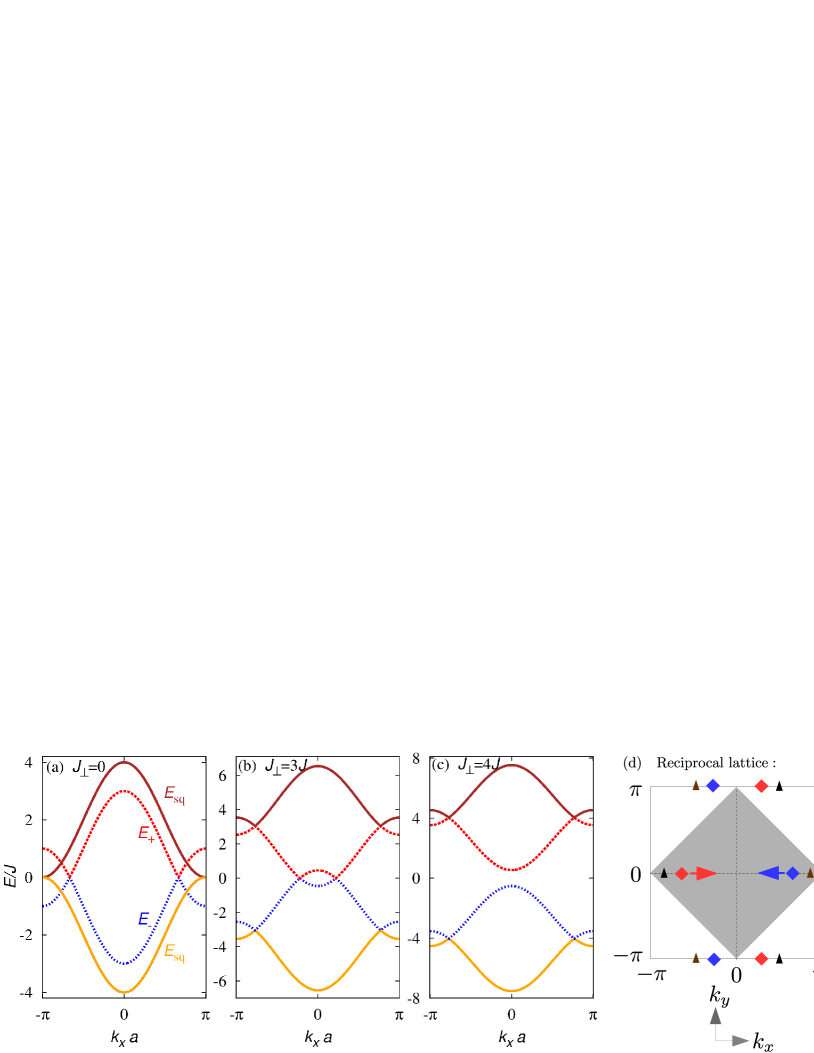
Due to translational invariance in the -plane, the eigenstates of are characterized by their wave vector . The real-space unit cell is spanned by vectors , and contains two sites per layer. This corresponds to a Brillouin zone as shown in Fig. 2, identical to the Brillouin zone of a brick-wall lattice, but half of the size of the square-lattice Brillouin zone. Reciprocal lattice vectors connecting equivalent points in -space are spanned by . Given two sublattices in each of the two layers, there are in total four eigenstates at each , that is, four bands form the band structure of the lattice. As we elaborate in this section, the band structure undergoes a topological transition upon tuning the interlayer coupling strength .
We start by considering the uncoupled system, . The band structure then consists of the two graphene bands , and the band of the square lattice :
| (3) | ||||
| (4) |
with the lattice spacing, set to 1 in the following. For simplicity, we choose . Naturally the square-layer band extends over a larger Brillouin than the brick-wall bands, but we can shift any point of the reciprocal lattice into the first Brillouin zone by . This shift splits the square-layer dispersion into two branches. A cross section of the band structure along is plotted in Fig.2(a). The bands from the brick-wall lattice and , depicted in blue and red, respectively, touch each other in Dirac points at momenta . Within the first Brillouin zone, we have a single pair of Dirac points at zero energy. Of course, the bands also look gapless at conical intersections between the square lattice band (brown and orange solid line in Fig. 2(a)) and the brick-wall lattice bands. However, it is important to note that no gapless excitations live at these intersections. A gapless excitation would correspond to a particle hopping from the brick-wall to the square lattice or vice versa, which is impossible for .
This is qualitatively different in the presence of a finite coupling between the layers: A gap opens at the conical intersections, except for two separated points in -space. These points now provide additional Dirac points, with gapless excitations, and linear dispersion along any direction in -space. We have also calculated the Berry phase for each of the bands along a contour encircling these intersection points, . At any finite , we obtain , thus the intersection points indeed are topologically protected Dirac points. We also note that the position of the intersection points is independent from the coupling , given by . At each of these two points, we have one band-touching at negative energy , between the first and the second band, and one at positive energy , between the third and the fourth band. Here we have introduced the short-hand notation
| (5) |
In order to have these Dirac points at the Fermi surface, we need to adjust the filling factor to for the Dirac points at negative energy, or for the Dirac points at positive energy. At these filling factors, the non-interacting system exhibits a semi-metallic phase for any finite value of . The Fermi velocity around these Dirac points is anisotropic. Along the -axis, we have , with , where is a unit of velocity. Along the -axis, we have , with .
In contrast to the intersection points, the Dirac excitations directly originating from the brick-wall lattice do not remain at fixed -positions upon changing the interlayer coupling, but their energy is pinned to . At any , they are located between the second and the third bad, i.e. they correspond to filling 1/2. While their position remains pinned at , their -position is parametrized as
| (6) |
that is, they move towards the center of the Brillouin zone when is increased, see Fig. 2(b). At a critical coupling , the two Dirac points merge at . For even larger values of the coupling, a gap opens and the Dirac points disappear, as shown in 2(c). The fact that the Dirac points can only merge at a high symmetry point of the Brillouin zone (here the center) is a generic feature, occurring as well in single-layered deformed honeycomb lattices [29, 30, 39].
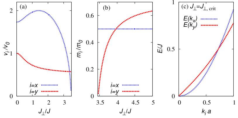
The non-interacting system at half filling thus undergoes a semi-metal to band insulator transition at . Near criticality the system exhibits some remarkable, highly anisotropic features: In the semi-metallic phase excitations are characterized by the Fermi velocities, which along the two lattice axes read:
| (7) | ||||
| (8) |
for . In the insulating phase the dispersion relation are massive , and the excitations are characterized by their effective mass , which again depends on the lattice direction. We obtain
| (9) | ||||
| (10) |
for . Here we have introduced as a unit of mass. The insulating gap reads
| (11) |
We have plotted the Fermi velocities and effective masses in Fig. 3 (a) and (b). While decreases smoothly to zero when the critical coupling is reached, remains non-zero even at the critical point, and drops to zero abruptly for larger values of . On the other hand, the effective mass along is zero at the critical point, and continuously increases for larger , while takes a constant finite value for any . At the critical point, this gives rise to the coexistence of massless excitations along , and massive excitations along , as illustrated in Fig. 3 (c). Such behavior has also been predicted in single-layered graphene-like systems [39, 40, 18]
Experimentally, the existence and position of Dirac points can be probed by accelerating the atomic cloud via a magnetic field gradient. If the atoms pass a Dirac point, there is transfer between the bands, which becomes visible in the quasi-momentum distribution after a Bragg reflection. This method has been pioneered in Ref. [18].
4 Superfluidity in bilayer system with attractive interactions
In the previous section, we considered the single particle (free) physics characterizing the coupled-layer system. This can be obtained by loading the lattice with spinless or fully spin-polarized fermionic atoms. In the following sections, we will consider the bilayer lattice loaded with two species of fermions, defining a pseudospin-1/2 degree of freedom (denoted by and ). Then, the fermions may interact, as described by the Hamiltonian . In the present section, we consider the case of weak attractive interactions ().
It is known that for uncoupled layers a pairing instability, captured by BCS theory, occurs in both the square and the brick-wall lattice, giving rise to a superfluid phase. However, while fermions in the square lattice form a superfluid at any attractive interaction [19], a peculiarity happens in the brick-wall lattice. At half filling (), the Dirac points are located on the Fermi surface, and below a critical interaction strength , the system remains in a semi-metal phase [41, 42].
To make predictions for the coupled layers, we follow the procedure of standard BCS theory, that is, we treat the interacting Hamiltonian on a mean-field level. To connect our results to the uncoupled case, we separately study the gap parameter on the brick-wall lattice, , and the gap parameter on the square lattice . In these expressions, the factor stems from the number of sites per sublattice (with the total number of sites). The BCS Hamiltonian then reads
| (12) |
In this notation we have introduced , and , with the intralayer hopping strength. Note that , such that the matrix is Hermitian. The parameter is a shifted chemical potential, which shall absorb the corresponding mean-field terms , , , and . We simplify our analysis by asking that takes identical values in both layers. With this restriction, we can only control the total particle number, but not the number of particles in each layer. We also disregard a possible spin dependence of , which renders the Hamiltonian symmetric under spin flips. We can therefore neglect the summation over .
The Hamiltonian is particle-hole symmetric, , where denotes particle-hole conjugation. Thus, the energy spectrum is symmetric around . The eigenstates at positive energy describe quasi-particle excitations, and the many-body ground state is the quasi-particle vacuum . We denote the quasi-particle operators by , where the different types of excitations are captured by the index running from 1 to 3. The corresponding energies are denoted . In this notation the Hamiltonian reads:
| (13) |
Explicitly, the quasi-particle operators are given by
| (14) |
and similarly for , with the coefficients and obtained from diagonalization of .
Once these coefficients are known, we can evaluate the number of particles and the pairing gap. By rewriting the original operators in terms of quasi-particle operators, it is straightforward to evaluate expectation values with respect to quasi-particle states. In the simplest case, at zero temperature, we just have to take the average with respect to the quasi-particle vacuum . We obtain:
| (15) |
and the same expressions for , , and with the upper indices on the right-hand-side replaced accordingly. Similarly, we have
| (16) |
and the corresponding expressions for , , and .
The equations (15) and (16), and their analogs for , , and can then be inserted into the gap equations. Restricting ourselves to zero temperature, we have
| (17) | ||||
| (18) |
and the number equation for the filling per site
| (19) |
Here, the summations shall cover the first Brillouin zone of the bilayer [see 2 (d)].
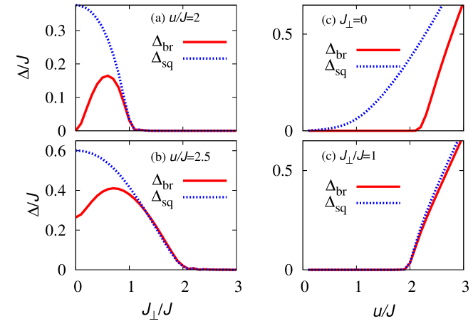
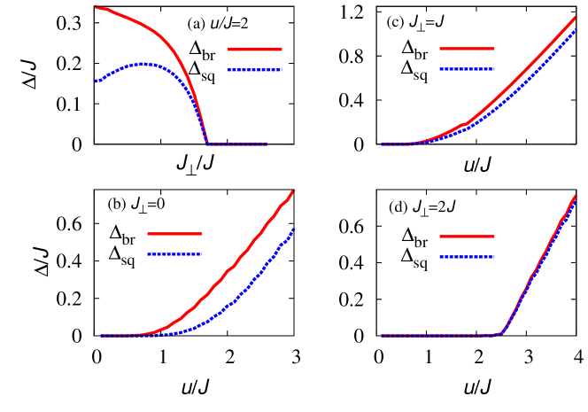
We first consider a system at half filling (), for which the number equation is solved by setting , independently of the gap parameters and . The gap equations are then solved iteratively. The results are illustrated in Fig. 4. Let us first comment on panel (c) which shows the behavior for two uncoupled layers, . As expected, the square lattice exhibits a finite gap, , at any finite value of . In contrast, the gap in the brick-wall layer remains zero up to a critical interaction strength (in units of used throughout the discussion). This behavior corresponds to the previously mentioned quantum phase transition from a semi-metal to a superfluid phase. Panel (d) of Fig. 4 shows the gaps as a function of for a finite value of . Here, both layers behave approximately the same, exhibiting a semi-metal to superfluid transition. In comparison to the transition in a single brick-wall layer, the critical interaction strength is slightly reduced, . So at the same time, the interlayer coupling suppresses superfluid correlations in the square layer, and favors superfluid correlations in the brick-wall layer.
This interpretation can also be drawn from panels (a) and (b) of Fig. 4, showing the gaps for fixed values of as a function of . In (a), with , the brick-wall layer is in the semi-metal phase in the limit of , but a finite coupling immediately establishes a finite pairing gap in both layers. Up to a certain value of , the brick-wall layer gap is further enhanced by the coupling, while the square layer gap always decreases with . For large , both gaps become strongly suppressed. The same behavior is seen also in panel (b) at , with only one qualitative difference seen in the uncoupled case, . At this interaction strength, also the uncoupled brick-wall layer is superfluid.
In summary, the half-filled bilayer behaves qualitatively the same way as a half-filled brick-wall lattice. In both cases, the Dirac point at the Fermi surface causes a semimetal to superfluid transition at finite . One might ask which role is played by the additional Dirac points at non-zero energy. Therefore, we first notice that they are at the Fermi surface for filling or filling . Here we shall note that, due to particle-hole symmetry, the fillings and are equivalent. We also note that, away from , solving gap and number equations self-consistently is considerably more difficult, as also the chemical potential depends on the gap.
Our main results are shown in Fig. 5. In the absence of interlayer coupling, shown in panel (b), both layers exhibit superfluid correlations for any non-zero strength of attractive interactions. Panel (a) shows that, upon turning on a sufficiently strong interlayer coupling, these superfluid correlations are suppressed. Interestingly, while for intermediate couplings, superfluid correlations can still be observed for arbitrarily small , cf. panel (c) with , stronger couplings require a finite interaction strength in order to establish a superfluid gap. Such scenario is illustrated in panel (d) with . Thus, for strong enough interlayer coupling, the system again exhibits a semi-metal to superfluid transition at filling one-fourth, .
To conclude this section, we should mention that at half filling, the superfluid correlations are exactly degenerate with charge density wave correlations in the attractive Hubbard model on bipartite lattices (such as e.g. the lattice in this paper). This is most easily seen by performing a particle-hole transformation on one species of spins, say , where ). This transformation converts the attractive Hubbard model at arbitrary filling into the repulsive Hubbard model at half filling in a magnetic field that couples to the -component of the spin [43, 44, 45, 46, 47]. The superfluid correlations in the attractive model then map onto spin correlations in the plane of the repulsive model, while charge density wave correlations map on to spin correlations in the -direction. Now, if also the attractive Hubbard model is at half filling, the effective magnetic field in the repulsive model is zero, revealing an additional SU(2) symmetry of the original model. This rotational symmetry implies the degeneracy between superfluid and density wave phase. Hence, at half filling, even though we have only considered superfluid correlations, one must keep in mind that the ground state has the peculiar property of simultaneous long range phase coherence (superfluid) and density order.
The charge density wave - superfluid state degeneracy is however broken on moving away from half filling, that is for a non-zero effective magnetic field in the repulsive Hubbard model, with the superfluid state always appearing to be energetically favorable (with the density wave correlations becoming short ranged) on the square [46, 48] and honeycomb lattices [49, 41]. On the other hand, longer range, i. e. off-site, interactions may stabilize charge density wave order or induce phase separation [43, 44, 45]. However we do not consider such interactions in the paper. In light of the above, we have focused on the generic instabilities of the studied model, that is pairing.
5 The brick-wall/square bilayer Heisenberg antiferromagnet
In this section, we will study the bilayer system with repulsive interactions, . At half filling, i.e. when the total number of particles is equal to the number of lattice sites , the system is in a Mott insulating phase for sufficiently large . In the perturbative limit, where , the low energy physics of the system is described by an effective spin-1/2 effective isotropic antiferromagnetic Heisenberg Hamiltonian
| (20) |
The indices now collect both the position of the spins in the plane, and with respect to the layer. The antiferromagnetic (superexchange) coupling arises from the virtual hopping of fermions in the sector of no doubly occupied states constituting the degenerate manifold of states describing the ideal Mott state corresponding to . Explicitly, it reads
| (21) |
We recall that at sufficiently low temperature, the isotropic Heisenberg antiferromagnet on hypercubic lattices is characterized by long-range antiferromagnetic order [50]. Despite the very low temperature scale set by the superexchange interactions, antiferromagnetic correlations have recently been observed in several experiments using Fermi gases in optical lattices [51, 52, 53, 54, 55, 56, 57]. Bipartite lattices in dimensions , such as square and brick-wall lattices, exhibit ground state Néel order [58, 59]. Strictly 2-dimensional and quasi 2-dimensional layered Heisenberg antiferromagnets have been routinely studied motivated in part due to possible relevance to the physics of high-Tc superconductivity. The square-lattice bilayer Heisenberg antiferromagnet is interesting because it can be driven through an order-disorder quantum phase transition [60, 61] by increasing the inter-plane coupling realizing a lattice model instance of the continuum field theory physics described by the (2+1)-dimensional non-linear model. It was suggested that certain magnetic properties of cuprate superconductors are reminiscent of those of a magnetic state close to such a quantum critical point [62, 63, 64]. On the other hand, such spin Hamiltonians are also relevant to the description of so-called spin dimer compounds which are magnetically disordered (pairs of spins bind together into singlets) but fascinatingly may be driven to order in a magnetic field via Bose-Einstein condensation of magnons [65, 66].
The inequivalent bilayer structure considered in this paper may be realized in an optical lattice setup as discussed in the next section, which warrants the study of the associated Heisenberg model (20). For interplane coupling , the system consists of two decoupled Néel ordered planes, although here each plane is characterized by a different value of the staggered magnetization. In the thermodynamic limit, the staggered magnetization per site in the square lattice is (see Ref. [58]) while the lower coordination number in the brick-wall lattice leads to a moderate decrease to the value (see Ref. [59]) due to enhanced effects of quantum fluctuations. Coupling the two lattices leads to an antiferromagnetically ordered two-layer system. In the opposite limit of , neighboring spins across the two layers are coupled to form isolated singlets or dimers. The excitation spectrum in the dimer phase is gapped, while it is gapless in the ordered phase. We restrict here to the evaluation of the critical coupling separating these two phases of the system. We mention that the two coupled square layers and two coupled brick-wall layers have been studied before yielding values (see Refs. [60, 67]) and (see Ref. [61]), respectively.
Since the system is bipartite, quantum Monte Carlo simulations can be performed without a sign problem. We use the projector Monte Carlo sampling method in the valence bond basis (we consider an even number of sites per layer) introduced by Sandvik [68] to obtain the ground state characteristics. We consider two coupled layers (a square and a brick-wall layer) containing sites with a square aspect ratio, so that the total number of sites is . In order to ensure convergence of observables to the ground state values, the projection length in the algorithm is chosen to be as high as . Performing the simulations in the valence-bond basis allows to access rotationally invariant correlation functions of the system (see e.g. Ref. [69]). In order to distinguish the Néel from dimer ordered phase, we consider the Néel structure factor (or square of staggered magnetization) of both the full lattice as well as for each layer separately. The staggered magnetization is defined as
| (22) |
where the sum is over either all lattice sites or those pertaining only to a single layer and is the number of spins in the considered system ( for the whole system and when considering a single layer. The staggering variable is a sublattice parameter – on dividing the total bipartite lattice in sublattices and , for sites on one sublattice for the other lattice. The structure factor is then defined as
| (23) |
corresponding to ordering at the the wave vector .
In order to locate the quantum critical point, we perform finite-size scaling of . Spin-wave theory predicts [70] the following finite size scaling of the magnetization for an ordered state:
| (24) |
where is the linear size of the system. Similarly, chiral perturbation theory and renormalization group calculations for the non-linear model yield the same form of finite size scaling [58]. Hence this form can be used to estimate the thermodynamic limit value of the staggered magnetization.
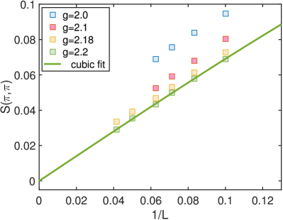
The scaling form (24) is well reflected in the obtained Monte Carlo data for the two-layer magnetization data as seen in Fig. 6. Deep in the Néel phase, e.g. for the inter- to intra-plane coupling ratio the dominant leading order finite size correction is clearly of the order of for the system sizes considered. On increasing the higher-order corrections become more important for lower system sizes. For , we find a polynomial of degree in the inverse systems size fits the data well. The value of the structure factor extrapolated to the thermodynamic limit is close to zero for . Hence we estimate the quantum critical point to be for this model.
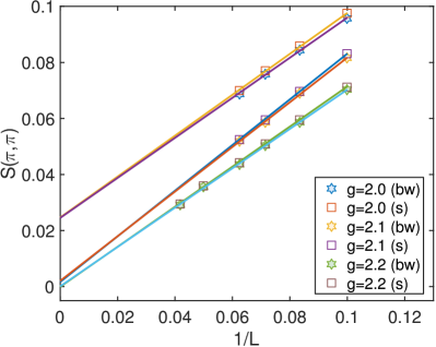
It is interesting to consider the in-plane magnetization of the two layers. We note that while for decoupled planes, the magnetizations of each layer is different, strong interlayer coupling is seen to make the magnetization uniform in both layers (see Fig. 7). For example, for , while the finite size values of the in-plane structure factor in the square lattice is always slightly higher than in the brick-wall layer, the extrapolated thermodynamic values are the same within the accuracy of the calculations (see Fig. 7) – top two lines). The in-plane structure factors also lead to conclusions in agreement with the estimate of the quantum critical point from the total system magnetization. As can be seen in Fig. 7, the Néel-to-dimer phase transition at is associated with the vanishing of the staggered magnetization in the two layers simultaneously.
6 Optical lattice implementation
Realizing these bilayers in solid-state systems, and tuning the coupling strength between the square and brick-wall layers is challenging. Fermi gases in optical lattices offer an interesting alternative where the system parameters can be freely adjusted. In the following we show that square/brick-wall bilayers can be generated using an extension of the optical lattice setups already used to realize brick-wall [18] and double-well lattices [71, 72, 73].
The key ingredient of the experimental implementation that we propose is a laser setup generating an optical lattice potential which alternates between square and brick-wall lattice structures when moving along the direction. It can be obtained through the addition of two independent potentials, designed in the following by and .
is created by the interference of the four retro-reflected beams sketched in Fig. 8(a). Two retro-reflected beams propagate in the plane along and have in-plane polarization, whereas two other beams propagate in the plane along and have out-of-plane polarization. Their wavelength is chosen to be red-detuned with respect to the atomic transitions. Hence, the atoms are trapped in the intensity maxima of the light. When setting the time-phase between the four beams to zero, e.g. by using standard phase-stabilization schemes (as in Refs. [74, 75, 18, 76]), the optical potential reads
| (25) |
where and denote the single-beam lattice depths and is the laser wavevector. Superimposing a standard square lattice potential in the plane
| (26) |
results in the desired succession of brick-wall and square planes for and respectively (where is an integer index) when choosing adequate values of the single-beam lattice depths. For instance, Fig. 8(b) displays the potential obtained for and . Note that, in order to simplify the experimental implementation, can be realized using the same beam wavelength and geometry as , but including only the running-wave beams. Then, a small frequency detuning between the beams leading to the different potentials is required in order to avoid unwanted cross-interference terms. Furthermore, the relative position of the and potentials in the plane needs to be adjusted (which can be achieved similarly to Ref. [20]).
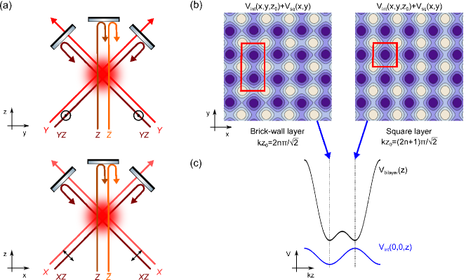
Finally, to get the desired bilayer structure we add an independent bichromatic optical lattice along with lattice depths and , and wavevectors and
| (27) |
It selects the planes in which the atoms are trapped and imprints a bilayer pattern along , as shown in Fig. 8(c). Tunneling between bilayers is suppressed by a strong potential barrier, whereas tunneling between two layers of each bilayer structure can be flexibly controlled by adjusting the ratio . The wave vectors and must be chosen such that the two potential minima of each bilayer coincide with a maximum and a minimum of , a situation which is realized for . As shown in Fig. 8(c), the total optical potential results in a square lattice in one minimum of each bilayer, and a brick-wall lattice in the other minimum with matching positions of the potential minima in both layers.
For fermionic 6Li atoms the lattice potential can be generated for instance with laser beams at nm, nm and nm, which have the correct wavelength relations and are all red-detuned with respect to the and transitions at nm. A polarized gas can be used to probe the lattice band structure and the properties of the Dirac points using a combination of Bloch oscillations and interband transitions as in Ref. [18]. Interactions can then be adjusted to both attractive and repulsive values using the broad Feshbach resonances available in the three lowest Zeeman sublevels [77]. In the attractive case, evidence for superfluidity could be obtained by observing interference peaks in time-of-flight images after sudden release from the optical lattice [78]. However, attaining the required temperatures in the Hubbard regime remains challenging. The repulsive case is more favorable, and recent experiments have already demonstrated the emergence of short-range magnetic correlations in various dimensionalities (although long-range magnetic order has not yet been observed). The experiments use either site merging [51, 53], Bragg scattering [52], or high resolution in-situ imaging [54, 55, 56, 57] to directly measure the singlet fraction, the spin structure factor, and spin-spin correlation functions. They thus allow for a comprehensive characterization of the magnetic properties of each layer, as well as of the singlet correlations expected between them in the limit of very large interlayer coupling.
7 Summary
We have considered a bilayer system with combined brick-wall and square lattice geometry. In this setting which can be realized with cold atoms in optical lattices, the brick-wall layer represents artificial graphene with semi-metal band structure, while the square layer exhibits a normal (metallic) band structure.
First, we have investigated how the coupling between the layers modifies the band structure. The Dirac points stemming from the brick-wall layer are shifted in -space, and merge at . At larger coupling, a gap is opened, thus the semi-metallic behavior is replaced by band-insulating behavior. At criticality, the excitations show exotic anisotropic features: Along one lattice direction, they remain massless, while in the other direction, they are massive. Additional Dirac points arise from the intersection of brick-wall and square lattice dispersion. Their position in -space is independent from the (finite) strength of the coupling .
Second, we have studied superfluidity of the system in the case of attractive interactions, using a mean-field approach. Similar to a single brick-wall layer at half filling, we find a semi-metal to superfluid transition of the bilayer. In the bilayer, such transition not only occurs at filling 1/2, but also at fillings 1/4 and 3/4 when the additional Dirac points appear at the Fermi surface.
Third, we have studied the case of strong repulsive interactions, in which the half-filled system is in the Mott phase, and can be mapped onto a Heisenberg antiferromagnet. Using the quantum Monte Carlo method, we have studied the behavior upon tuning the interlayer coupling. For , we find a phase transition from magnetic long-range order within the planes to a valence bond crystal with strong dimers between the layers.
Finally, we have presented a possible experimental implementation which is readily accessible in experiments with Fermi gases in optical lattices using state-of-the-art technology, and discussed perspectives for observing experimentally these phases.
Beyond its relevance for artificial graphene systems discussed here, our approach for generating an atomic bilayer system provides a general new tool for studying proximity effects with cold atoms. Future work may combine the bilayer scenario of this paper with ideas from a recent proposal where parafermions emerge in a heterostructure of a Bose-Einstein condensate and a fractional quantum Hall system [79].
References
- [1] K. S. Novoselov et al., Nature 490, 192 (2012).
- [2] A. H. Castro Neto et al., Rev. Mod. Phys. 81, 109 (2009).
- [3] K. S. Novoselov et al., Nat. Phys. 2, 177 (2006).
- [4] C. Ortix, L. Yang, and J. van den Brink, Phys. Rev. B 86, 081405 (2012).
- [5] M. Yankowitz et al., Nat. Phys. 8, 382 (2012).
- [6] A. Principi et al., Phys. Rev. B 86, 085421 (2012).
- [7] A. Gamucci et al., Nat. Comm. 5, (2014).
- [8] I. Aliaj et al., APL Mater. 4, (2016).
- [9] M. Polini et al., Nat. Nano. 8, 625 (2013).
- [10] C.-H. Park and S. G. Louie, Nano Letters 9, 1793 (2009).
- [11] A. Singha et al., Science 332, 6034 (2011).
- [12] S. Wang et al., submitted to APL (2016).
- [13] K. K. Gomes et al., Nature 483, 306 (2012).
- [14] R. A. Sepkhanov, Y. B. Bazaliy, and C. W. J. Beenakker, Phys. Rev. A 75, 063813 (2007).
- [15] M. C. Rechtsman et al., Phys. Rev. Lett. 111, 103901 (2013).
- [16] U. Kuhl et al., Phys. Rev. B 82, 094308 (2010).
- [17] P. Soltan-Panahi et al., Nat. Phys. 7, 434 (2011).
- [18] L. Tarruell et al., Nature 483, 302 (2012).
- [19] M. Lewenstein, A. Sanpera, and V. Ahufinger, Ultracold Atoms in Optical Lattices - Simulating quantum many-body systems (Oxford University Press, New York, 2012).
- [20] G.-B. Jo et al., Phys. Rev. Lett. 108, 045305 (2012).
- [21] L. Duca et al., Science 347, 288 (2015).
- [22] T. Li et al., Science 352, 1094 (2016).
- [23] M. Weinberg et al., 2D Materials 3, 024005 (2016).
- [24] T. Uehlinger et al., EPJ ST 217, 121 (2013).
- [25] T. Uehlinger et al., Phys. Rev. Lett. 111, 185307 (2013).
- [26] G. Jotzu et al., Nature 515, 237 (2014).
- [27] N. Fläschner et al., Science 352, 1091 (2016).
- [28] S.-L. Zhu, B. Wang, and L.-M. Duan, Phys. Rev. Lett. 98, 260402 (2007).
- [29] B. Wunsch, F. Guinea, and F. Sols, New J. Phys. 10, 103027 (2008).
- [30] K. L. Lee et al., Phys. Rev. A 80, 043411 (2009).
- [31] D. Poletti, C. Miniatura, and B. Grémaud, EPL 93, 37008 (2011).
- [32] D.-S. Lühmann et al., Phys. Rev. A 90, 013614 (2014).
- [33] L. Cao et al., Phys. Rev. A 91, 043639 (2015).
- [34] R. M. Lutchyn, J. D. Sau, and S. Das Sarma, Phys. Rev. Lett. 105, 077001 (2010).
- [35] J. D. Sau, R. M. Lutchyn, S. Tewari, and S. Das Sarma, Phys. Rev. Lett. 104, 040502 (2010).
- [36] H.-Y. Hui, J. D. Sau, and S. Das Sarma, Phys. Rev. B 92, 174512 (2015).
- [37] W. S. Cole, J. D. Sau, and S. Das Sarma, arXiv/ 1603.03780 (2016).
- [38] D. Scarabelli et al., arxiv/1507.04390 (2015).
- [39] G. Montambaux, F. Piéchon, J.-N. Fuchs, and M. O. Goerbig, Phys. Rev. B 80, 153412 (2009).
- [40] P. Dietl, F. Piéchon, and G. Montambaux, Phys. Rev. Lett. 100, 236405 (2008).
- [41] E. Zhao and A. Paramekanti, Phys. Rev. Lett. 97, 230404 (2006).
- [42] S. Tsuchiya, R. Ganesh, and A. Paramekanti, Phys. Rev. A 86, 033604 (2012).
- [43] S. Robaszkiewicz, R. Micnas, and K. A. Chao, Phys. Rev. B 23, 1447 (1981).
- [44] S. Robaszkiewicz, R. Micnas, and K. A. Chao, Phys. Rev. B 24, 1579 (1981).
- [45] S. Robaszkiewicz, R. Micnas, and K. A. Chao, Phys. Rev. B 24, 4018 (1981).
- [46] A. Moreo and D. J. Scalapino, Phys. Rev. Lett. 66, 946 (1991).
- [47] A. F. Ho, M. A. Cazalilla, and T. Giamarchi, Phys. Rev. A 79, 033620 (2009).
- [48] D. J. Scalapino, S. R. White, and S. Zhang, Phys. Rev. B 47, 7995 (1993).
- [49] K. L. Lee et al., Phys. Rev. B 80, 245118 (2009).
- [50] E. Manousakis, Rev. Mod. Phys. 63, 1 (1991).
- [51] D. Greif et al., Science 340, 1307 (2013).
- [52] R. A. Hart et al., Nature 519, 211 (2015).
- [53] D. Greif et al., Phys. Rev. Lett. 115, 260401 (2015).
- [54] M. F. Parsons et al., Science 353, 1253 (2016).
- [55] M. Boll et al., Science 353, 1257 (2016).
- [56] L. W. Cheuk et al., Science 353, 1260 (2016).
- [57] J. H. Drewes et al., arXiv/1607.00392 (2016).
- [58] A. W. Sandvik, Phys. Rev. B 56, 11678 (1997).
- [59] E. V. Castro, N. M. R. Peres, K. S. D. Beach, and A. W. Sandvik, Phys. Rev. B 73, 054422 (2006).
- [60] A. W. Sandvik and D. J. Scalapino, Phys. Rev. Lett. 72, 2777 (1994).
- [61] R. Ganesh, S. V. Isakov, and A. Paramekanti, Phys. Rev. B 84, 214412 (2011).
- [62] S. Sachdev and J. Ye, Phys. Rev. Lett. 69, 2411 (1992).
- [63] A. V. Chubukov and S. Sachdev, Phys. Rev. Lett. 71, 169 (1993).
- [64] A. Sokol and D. Pines, Phys. Rev. Lett. 71, 2813 (1993).
- [65] T. Nikuni, M. Oshikawa, A. Oosawa, and H. Tanaka, Phys. Rev. Lett. 84, 5868 (2000).
- [66] T. Giamarchi, C. Rüegg, and O. Tchernyshyov, Nat. Phys. 4, 198 (2008).
- [67] L. Wang, K. S. D. Beach, and A. W. Sandvik, Phys. Rev. B 73, 014431 (2006).
- [68] A. W. Sandvik, Phys. Rev. Lett. 95, 207203 (2005).
- [69] Y.-J. Lin et al., Nature 462, 628 (2009).
- [70] D. A. Huse, Phys. Rev. B 37, 2380 (1988).
- [71] J. Sebby-Strabley, M. Anderlini, P. S. Jessen, and J. V. Porto, Phys. Rev. A 73, 033605 (2006).
- [72] S. Fölling et al., Nature 448, 1029 (2007).
- [73] J. Li et al., Phys. Rev. Lett. 117, 185301 (2016).
- [74] A. Hemmerich, D. Schropp, T. Esslinger, and T. W. Hänsch, Eur. Phys. Lett. 18, 391 (1992).
- [75] M. Greiner et al., Phys. Rev. Lett. 87, 160405 (2001).
- [76] T. Kock, C. Hippler, A. Ewerbeck, and A. Hemmerich, J. Phys. B 49, 042001 (2016).
- [77] G. Zürn et al., Phys. Rev. Lett. 110, 135301 (2013).
- [78] J. K. Chin et al., Nature 443, 961 (2006).
- [79] M. F. Maghrebi et al., Phys. Rev. Lett. 115, 065301 (2015).