Finite sample bounds for expected number of false rejections under martingale dependence with applications to FDR.

Abstract

Much effort has been made to improve the famous step up test of Benjamini and Hochberg given by linear critical values $\frac{i\alpha}{n}$. It is pointed out by Gavrilov, Benjamini and Sarkar that step down multiple tests based on the critical values $\beta_{i}=\frac{i\alpha}{n+1-i(1-\alpha)}$ still control the false discovery rate (FDR) at the upper bound $\alpha$ under basic independence assumptions. Since that result in not longer true for step up tests or dependent single tests, a big discussion about the corresponding FDR starts in the literature. The present paper establishes finite sample formulas and bounds for the FDR and the expected number of false rejections for multiple tests using critical values $\beta_{i}$ under martingale and reverse martingale dependence models. It is pointed out that martingale methods are natural tools for the treatment of local FDR estimators which are closely connected to the present coefficients $\beta_{i}.$ The martingale approach also yields new results and further inside for the special basic independence model.

and

t1Partially suppoted by SAW-Project ”Multiplizität, Modellvalidierung und Reproduzierbarkeit in hochdimensionalen Microarray-Daten”

1 Introduction

Multiple tests are nowadays well established procedures for judging high dimensional data. The famous Benjamini and Hochberg [2] step up multiple test given by linear critical values controls the false discovery rate FDR for various dependence models. The FDR is the expectation of the ratio of the number of false rejections devided by the amount of all rejected hypotheses. For these reasons the linear step up test is frequently applied in practice. Gavrilov et al. [11] pointed out that linear critical values can be substituted by

$$\beta_{i}=\frac{i\alpha}{n+1-i(1-\alpha)},\ i\leqslant n,$$ (1.1)

for step down tests and the FDR control (i.e. FDR$\leqslant\alpha$) remains true for the basic independence model of the underlying p-values. Note that the present critical values $\beta_{i}$ are closely related to critical values given by the asymptotic optimal rejection curve which is obtained by Finner et al. [8]. In the asymptotic set up they derived step up tests with asymptotic FDR control under various conditions. However, step up multiple tests given by the $\beta_{i}$’s do not control the FDR by the desired level $\alpha$ at finite sample size, see for instance Dickhaus [7], Gontscharuk [12].
The intension of the present paper is twofold.

• We like to calculate the FDR of step down and step up tests more precisely using martingale and reverse martingale arguments. Here we get also new results under the basic independence model.

• On the other hand we can extend the results for dependent p-values which are martingale or reverse martingale dependent. As application finite sample FDR formulas for step down and step up tests based on (1.1) are derived. We refer to the Appendix for a collection of examples of martingale models.

Martingale arguments were earlier used in Storey et al. [22], Pena et al. [17], Heesen and Janssen [14] for step up and in Benditkis [1] for step down multiple tests.
This paper is organized as follows. Below the basic notations are introduced. Section 2 presents our results for step down tests. A counterexample, Example 4, motivates to study specific dependence concepts which allow FDR control, namely our martingale dependence model. The FDR formula, see (1.7) below, consists of two terms. In particular, it relies on the expected number of false rejections which is studied in Sections 2.1 and 2.2. Note that the results of Lemma 6 motivate naturally the consideration of martingale methods. Section 2.3 is devoted to the FDR control under dependence which extends the results of Gavrilov et al. [11]. Within the class of step down tests the first coefficient $\beta_{1}$ is often responsable for the quality of the multiple test. In Section 2.4 we propose an improvement of the power of SD procedures due to an increase of first critical values without loosing the FDR control.
Step up multiple tests corresponding to the $\beta$’s from (1.1) are studied in Sections 3 and 4. We obtain the lower bound for the present FDR which can be greater than $\alpha.$ A couple of examples for martingale models can be found in Appendix. The proofs and additional material are collected in the Section 5.

Basics. Let us consider a multiple testing problem, which consists of $n$ null hypotheses $H_{1},...,H_{n}$ with associated p-values $p_{i},\ i=1,...,n.$ Assume that all p-values arise from the same experiment given by one data set, where each $p_{i}$ can be used for testing the traditional null $H_{i}$. The p-values vector $p=(p_{1},...,p_{n})\in[0,1]^{n}$ is a random variable based on an unknown distribution $P.$ Recall that simultaneous inference can be established by so called multiple tests $\phi=\phi(p),$ $\phi=(\phi_{1},...,\phi_{n}):[0,1]^{n}\rightarrow\{0,1\}^{n},$ which rejects the null $H_{i}$ iff, i.e. if and only if, $\phi_{i}(p)=1$ holds. The set of hypotheses can be divided in the disjoint union $I_{0}\bigcup I_{1}=\{1,...,n\}$ of unknown portions of true null $I_{0}$ and false null $I_{1},$ respectively. We denote the number of true null by $n_{0}=|I_{0}|$ and the number of false ones by $n_{1}=|I_{1}|=n-n_{0},$ where $n_{0}>0$ is assumed. Widely used multiple testing procedures can be represented as

$$\phi_{\tau}=(\mbox{$\mathbb{I}$}(p_{1}\leqslant\tau),...,\mbox{$\mathbb{I}$}(p_{n}\leqslant\tau))$$

via the indicator function $\mbox{$\mathbb{I}$}(\cdot),$ where $\tau\in[0,1]$ is a random critical boundary variable. Thus all null hypotheses with related p-values that are not larger than the threshold $\tau$ have to be rejected. Let $p_{1:n}\leqslant p_{2:n}\leqslant\cdot\cdot\cdot\leqslant p_{n:n}$ denote the ordered values of the p-values $p$.

Definition 1.

Let $\alpha_{1}\leqslant\alpha_{2}\leqslant\cdot\cdot\cdot\leqslant\alpha_{n}$ be a deterministic sequence of critical values. Set for convenience $\max\{\emptyset\}=0.$

• The step down (SD) critical boundary variable is given by

  $$\tau_{SD}=\max\{\alpha_{i}:p_{j:n}\leqslant\alpha_{j},\text{ \ for \ all \ }j\leqslant i\}.$$ (1.2)

• The step up (SU) critical boundary variable is given by

  $$\tau_{SU}=\max\{\alpha_{i}:p_{i:n}\leqslant\alpha_{i}\}.$$ (1.3)

• The appertaining multiple tests $\phi_{SD}=\phi_{\tau_{SD}}$ and $\phi_{SU}=\phi_{\tau_{SU}}$ are called step down (SD) test, step up (SU) test, respectively.

Let $\hat{F}_{n}$ denote the empirical distribution function of the p-values and let $V=V(\tau)=\sum\limits_{i\in I_{0}}\mathbb{I}(p_{i}\leqslant\tau)$, $S=S(\tau)=\sum\limits_{i\in I_{1}}\mathbb{I}(p_{i}\leqslant\tau)$ and $R=R(\tau)=\sum\limits_{i=1}^{n}\mathbb{I}(p_{i}\leqslant\tau)=n\hat{F}_{n}(\tau)$ be the number $V$ of false rejections w.r.t. $\tau$, the number $S$ of true rejections and the number $R$ of all rejections, respectively. The False Discovery Rate (FDR) of a procedure with critical boundary variable $\tau$ is defined as

$$\text{FDR}={\mathbb{E}}\left[\frac{V(\tau)}{R(\tau)}\right],$$

with the convention $\frac{0}{0}=0$. The FDR is often chosen as an error rate control criterion. There is another useful equivalent description of step down tests.

Remark 2.

Introduce the random variable

$$\sigma:=\min\{\alpha_{i}:p_{i:n}>\alpha_{i}\}\wedge\alpha_{n},$$ (1.4)

where $a\wedge b=\min(a,b)$ denotes the minimum of two real numbers $a$ and $b.$

Then we have $\tau_{SD}\leqslant\sigma$ but the step down tests $\phi_{SD}=\phi_{\sigma}$ coincide and $\text{FDR}={\mathbb{E}}\left[\frac{V(\tau_{SD})}{R(\tau_{SD})}\right]={\mathbb{E}}\left[\frac{V(\sigma)}{R(\sigma)}\right]$ holds. The reason for this is that no p-value falls in the interval $(\tau_{SD},\sigma]$ and $R(\tau_{SD})=R(\sigma)$ is valid.

There is much interest in multiple tests such that the FDR is controled by a prespecified acceptable level $\alpha\in(0,1)$, i.e. to bound the expectation of the portion of false rejections. The well known so called Benjamini and Hochberg multiple tests with linear critical values $\alpha_{i}=\alpha\frac{i}{n}$ lead to the FDR bound

$$\text{FDR}\leqslant\alpha\frac{n_{0}}{n}$$

for SD and SU tests under positive dependence, more precisely under positive regression dependence on a subset (PRDS). There are several proposals to exhaust the FDR more accurate by $\alpha$ by an enlarged choice of critical values. A proper choice for SD tests are $\alpha_{i}$

$$\begin{aligned} &0<\alpha_{i}\leqslant\beta_{i}=\frac{i\alpha}{n+1-i(1-\alpha)},\ 1\leqslant i\leqslant n,\\ &\alpha_{0}=\alpha_{1},\ \beta_{0}=\beta_{1},\end{aligned}$$ (1.5)

which allow the control $\text{FDR}\leqslant\alpha$ under the basic independence assumption of the p-values, see Gavrilov et al. [11]. Note that for $i=1,...,n,$ $\beta_{i}=g_{\alpha}^{-1}\left(\frac{i}{n}\right)$ are inverse values of

$$g_{\alpha}(t)=\frac{n+1}{n}f_{\alpha}(t)=\frac{n+1}{n}\frac{t}{t(1-\alpha)+\alpha},$$ (1.6)

where $g_{\alpha}$ is close to the asymptotic optimal rejection curve $f_{\alpha},$ see Finner et al. [8]. It is known that SU tests given by $\beta_{i}$ do not control the FDR for the independence model in general, see Gontscharuk [12], Heesen and Janssen [14]. If the p-values are dependent then the FDR control of the SD tests based on $\beta_{i},\ i\leqslant n,$ can not be expected (see Example 4 of Section 2).
Gavrilov et al. [11], Theorem 1A, propose to reduce the critical values $\beta_{i}$ in order to get FDR control of SD-tests under positive regression dependence on a subset. Unfortunately, the procedure based on these new reduced critical values may be too conservative. Below we keep the critical values $\alpha_{i},\ i\leqslant n,$ of (1.5) and introduce dependence assumptions for the p-values which insure the FDR-control for the underlying SD tests.
The main idea of this paper can be outlined as follows. The FDR of SD and SU tests based on the critical values $\beta_{i}$ equals

$$\text{FDR}=\frac{\alpha}{n+1}{\mathbb{E}}\left[\frac{V}{\beta_{R}}\right]+\frac{1-\alpha}{n+1}{\mathbb{E}}\left[V\right].$$ (1.7)

A monotonicity argument implies the next Lemma.

Lemma 3.

Consider an SD or SU test with critical values $(\alpha_{i})_{i}$ given by (1.5). Then

• $\text{FDR}\leqslant\frac{\alpha}{n+1}{\mathbb{E}}\left[\frac{V}{\beta_{R}}\right]+\frac{1-\alpha}{n+1}{\mathbb{E}}\left[V\right]$.

• The conditions

  $${\mathbb{E}}\left[\frac{V}{\beta_{R}}\right]\leqslant n_{0}\text{ \ and \ }$$ (1.8)

  $${\mathbb{E}}\left[V\right]\leqslant\frac{\alpha}{1-\alpha}(n_{1}+1)$$ (1.9)

  ensure the FDR control, i.e. FDR$\leqslant\alpha.$

Whereas the FDR is hard to bound under dependence, the inequality (1.8) is known under PRDS and equality holds under reverse martingale structure (including the basic independence model), see Heesen and Janssen [14] for SU test. Then it remains to bound the expected number of false rejections ${\mathbb{E}}\left[V\right]$, which is at least possible for SD tests under certain martingale dependence assumptions. In the following we always use a general assumption, that the p-values for the true null $(H_{i})_{i\in I_{0}}$ fullfil

$${\mathbb{E}}\left[\sum\limits_{i\in I_{0}}\mbox{$\mathbb{I}$}(p_{i}\in[0,t])\right]\leqslant n_{0}t\text{ \ for \ all \ }t\in[0,1),$$ (1.10)

which can be interpreted as ”stochastically larger” condition compared with the uniform distribution in the mean for $I_{0}$.

Now, we define the basic independence assumptions (BIA) that are often used in the FDR-control-framework.

• We say that p-values fulfil the basic independence model if the vectors of p-values $\left(p_{i}\right)_{i\in I_{0}}$ and $\left(p_{i}\right)_{i\in I_{1}}$ are independent, and each dependence structure is allowed for the “false” p-values within $\left(p_{i}\right)_{i\in I_{1}}.$ Under true null hypotheses the p-values $\left(p_{i}\right)_{i\in I_{0}}$ are independent and stochastically larger (or equal) compared to the uniform distribution on $[0,1],$ i.e., $P(p_{i}\leqslant x)\leqslant x$ for all $x\in[0,1]$ and $i\in I_{0}.$
  If in addition all p-values are i.i.d. uniformly distributed on $[0,1]$ for $i\in I_{0}$ then we talk about the BIA model with uniform true p-values.

2 Results for step down procedures

In this section we consider a step down procedure with critical values $\beta_{i},\ i\leqslant n,$ from (1.1). It is well known that this procedure controls the FDR if the p-values fulfil the basic independence assumptions (BIA) (cf. Gavrilov et al. [11]). However, in practice the independence of the single tests corresponding to the present p-values are rare.

For general dependent p-values the FDR of the SD test may exceed the level $\alpha.$ The next counter example motivates the consideration of special kinds of dependence in order to establish FDR control.

Example 4.

For $n=3,\ n_{0}=2,\ n_{1}=1,\ I_{0}=\{2,3\}$ and $\alpha=\frac{1}{4}$ consider the SD procedure with critical values $\beta_{i}=\frac{i\alpha}{n+1-i(1-\alpha)}$. Consider the vector of p-values $\left(0,U_{1},U_{2}\right)$ with true p-values defined as follows

$$U_{1}\text{ \ is \ uniformly \ distributed \ on \ }(0,1).$$

$$U_{2}=\left(U_{1}+\beta_{2}\right)\mbox{$\mathbb{I}$}\left(U_{1}\leqslant\beta_{2}\right)+\left(U_{1}-\beta_{2}\right)\mbox{$\mathbb{I}$}\left(U_{1}\in(\beta_{2},2\beta_{2})\right)+U_{1}\mbox{$\mathbb{I}$}\left(U_{1}\geqslant 2\beta_{2}\right).$$

For such p-values we get

$$\text{FDR}=\frac{2}{3}P(U_{1}\leqslant 2\beta_{2})=\frac{4\beta_{2}}{3}=\frac{4}{15}>\frac{1}{4}.$$

We will start with the expected number of false rejections (ENFR), which was earlier studied by Finner and Roters [10] and Scheer [19].

2.1 Control of the expected number of false rejections ${\mathbb{E}}\left[V\right]$

The present martingale approach relies on the empirical distribution function $\hat{F}_{n}$ of the p-values and on the adapted stochastic process

$$\begin{aligned} t\mapsto\hat{\alpha}(t)=\frac{t}{1-t}\frac{1-\hat{F}_{n}(t)}{\hat{F}_{n}(t)+\frac{1}{n}},\ t\in T,\text{w.r.t. \ the \ filtration \ }\\ \mathcal{F}_{t}^{T}=\sigma\{\mbox{$\mathbb{I}$}(p_{i}\leqslant s),s\leqslant t,s,t\in T,\ i\leqslant n\}\text{ \ of \ the \ p-values}.\end{aligned}$$ (2.1)

Thereby, $T\subset[0,1)$ is a parameter space with $0\in T.$ The value $\hat{\alpha}(t)$ is frequentely used as a conservative estimator for the FDR on the constant critical boundary value $\tau=t.$ Storey et al. [21] use a similar estimator for the FDR$(t)$ of SU tests if the p-values are independent. A similar estimator is also used by Benjamini, Krieger and Yekutieli [3], Heesen and Janssen [15] and Heesen [13]. It is easy to see that for $\beta_{i},\ i\leqslant n,$ we get from (1.5)

$$\hat{\alpha}_{n}(\beta_{i})\leqslant\alpha\text{ \ iff \ }R(\beta_{i})\geqslant i-1,$$ (2.2)

$$\hat{\alpha}_{n}(\beta_{i})=\alpha\text{ \ iff \ }R(\beta_{i})=i-1,$$ (2.3)

since

$$\hat{\alpha}_{n}(\beta_{i})=\alpha\left(\frac{i}{n+1-i}\right)\left(\frac{n-R(\beta_{i})}{R(\beta_{i})+1}\right).$$

The consequences of these useful relations are summerized.

Lemma 5.

Consider the critical values $\left(\beta_{i}\right)_{i\leqslant n}$ and the critical boundary value $\sigma$ from (1.4). Then we have

• $\sigma=\min\{\beta_{i}:\hat{\alpha}_{n}(\beta_{i})\geqslant\alpha,i\leqslant n\}\wedge\beta_{n}.$

• Moreover $\tau_{SD}\leqslant\sigma$ and $\hat{\alpha}_{n}(\sigma)=\alpha\mbox{$\mathbb{I}$}(R(\sigma)<n)$ hold.

• The random variable $\sigma$ is a stopping time w.r.t. the filtration $\left(\mathcal{F}_{t}^{T}\right)_{t\in T}$ of the p-values with time domain $T=\{0,\beta_{1},...,\beta_{n}\}$.

It is quite obvious that the maximal coefficiens $\beta_{i},i\leqslant n,$ of the $\alpha^{\prime}s$ in (1.5) and the extreme p-values $p_{i}=0,\ i\in I_{1},$ for all false null are least favourable for bounding ${\mathbb{E}}\left[V\right].$ First, we focus on the $\beta_{i}-$based SD procedure. An important role plays the process

$$M_{t}=M_{I_{0}}(t)=\sum\limits_{i\in I_{0}}\frac{\mbox{$\mathbb{I}$}(p_{i}\leqslant t)-t}{1-t},\ t\in T.$$ (2.4)

Lemma 6.

Let $p_{i}=0\text{ \ for \ all \ }i\in I_{1}.$ For the critical values $(\beta_{i})_{i\leqslant n}$ from (1.1) we have

$${\mathbb{E}}\left[V(\tau_{SD})\right]\leqslant\frac{\alpha}{1-\alpha}(n_{1}+1)\text{ \ iff \ }{\mathbb{E}}\left[M_{I_{0}}\right]\leqslant\alpha(n+1)P(R(\tau_{SD})=n).$$

The probability $P(R(\tau_{SD})=n)$ is typically very small. Note that we will show below by martingale arguments that ${\mathbb{E}}\left[M_{I_{0}}(\tau_{SD})\right]\leqslant 0,$ which implies the crucial condition (1.9).

Next, we introduce a dependence assumption which allows the control of expected number of false rejection of the SD procedure with critical values $\beta_{i},i\leqslant n.$

• Let $T\subset[0,1)$ be a set with $0\in T$. We say that p-values $p_{1},...,p_{n}$ are $\mathcal{F}_{T}=\left(\mathcal{F}_{t}\right)_{t\in T}-$ (super-) martingale dependent on a subset $J$ if the stochastic process $M(t)=M_{J}(t)=\sum\limits_{i\in J}\left(\frac{\mbox{$\mathbb{I}$}(p_{i}\leqslant t)-t}{1-t}\right),t\in T,$ is a $\mathcal{F}_{T}-$ (super-)martingale.

Note that the super-martingale model (D1) includes BIA if $J=I_{0}$. This is well known, see Shorack and Wellner [20] (p. 133), Benditkis [1]. Some examples of martingale dependent random variables can be found in a separate Appendix.
Recall that the general condition (1.10) implies ${\mathbb{E}}\left[M_{I_{0}}(0)\right]=0,$ which is always assumed.
The next remark shows that under (D1) we can assume that the p-values which belong to true null are stochastically larger compared with the uniform distribution on $(0,1)$ (cf. Heesen and Janssen [14], Benditkis [1]). Let $U(0,1)$ denote the uniform distribution on the unit interval.

Remark 7.

Let $\left(p_{i}\right)_{i\leqslant n}$ fulfil the martingale assumption (D1) for $J=I_{0}$ on $T\subset[0,1]$ and let $\sigma:I_{0}\rightarrow I_{0}$ be some random permutation of the index-set $I_{0}$ which is independent of $\left(p_{i}\right)_{i\leqslant n}$.

• If

  $$M_{I_{0}}(t)=\sum\limits_{i\in I_{0}}\frac{\mbox{$\mathbb{I}$}(p_{i}\leqslant t)-t}{1-t}\text{ \ is \ a \ }\mathcal{F}_{T}-\text{martingale,}$$

  then the random variable $Y_{i}=p_{\sigma(i)},i\in I_{0},$ is U$(0,1)$-distributed.

• If $\left(p_{i}\right)_{i\in I_{0}}$ fulfil the super-martingale assumption (D1) for $J=I_{0}$ on $T\subset[0,1]$, then $Y_{i}$, $i\in I_{0},$ are stochastically larger compared with $U(0,1)$.

• As long as the boundary critical value $\tau$ only depends on the order statistics, the multiple test $\phi_{\tau}$ remains unchanged if $\left(p_{i}\right)_{i\leqslant n}$ is substituted by $\left((p_{\sigma(i)})_{i\in I_{0}},(p_{i})_{i\in I_{1}}\right).$

• It can be shown that under (D1) the (super-)martingale assumption also holds under the filtration given by the exchangeable $\left(\left(Y_{i}\right)_{i\in I_{0}},\left(p_{i}\right)_{i\in I_{1}}\right).$ Note that the exchangeability of the $p_{\sigma(i)},\ i\in I_{0},$ is only needed in the proofs in connection with the PRDS assumption introduced in Section 2.3.

Proof of (a) and (b).

Firstly, note that the random variables $Y_{i},i\in I_{0}$ are exchangeable, since $\sigma$ is an independent permutation. This implies

$${\mathbb{E}}\left[\mbox{$\mathbb{I}$}(Y_{i}\leqslant t)\right]={\mathbb{E}}\left[\frac{1}{n_{0}}\sum\limits_{i\in I_{0}}\mbox{$\mathbb{I}$}(Y_{i}\leqslant t)\right]={\mathbb{E}}\left[\frac{1}{n_{0}}\sum\limits_{i\in I_{0}}\mbox{$\mathbb{I}$}(p_{i}\leqslant t)\right].$$ (2.5)

Moreover, we get

$${\mathbb{E}}\left[\frac{1}{n_{0}}\sum\limits_{i\in I_{0}}\mbox{$\mathbb{I}$}(Y_{i}\leqslant t)\right]=\frac{(1-t)}{n_{0}}{\mathbb{E}}\left[M_{I_{0}}(t)\right]+t\leqslant t.$$ (2.6)

Note that we have an (in)equality in (2.6), if $M_{I_{0}}(t)$ is a $\mathcal{F}_{T}-$(super-)martingale. ∎

Now, we formulate the main result of this subsection under the super-martingale assumption, which will be applied to our equality (1.7).

Theorem 8.

Consider the SD multiple procedure with critical values $\beta_{i}$, $i\leqslant n$, given in (1.5). Suppose that the super-martingale assumption (D1) holds with $J=I_{0}$ and $T=\{0,\beta_{1},...,\beta_{n}\}$.We get

$${\mathbb{E}}\left[V(\tau_{SD})\right]\leqslant\frac{\alpha}{1-\alpha}({\mathbb{E}}\left[S(\tau_{SD})\right]+1)\leqslant\frac{\alpha}{1-\alpha}(n_{1}+1).$$

2.2 Consequences under Dirac-Martingale configurations

In this subsection we consider the following assumptions

• Martingale dependence assumption (D1) holds with $J=I_{0}\ \text{and}\ T=\{0,\beta_{1},...,\beta_{n}\}$,

• $p_{i}=0$ a.s. for all $i\in I_{1}$.

Structures that fulfil the assumptions (i) and (ii) are called Dirac martingale configurations DM($n_{1}$). The part (a) of the next lemma proposes exact formulas for ENFR for step down tests with critical values $\beta_{i}.$ Part (b) derives a lower bound for ENFR if the $(p_{i})_{i\in I_{1}}$ are by accident uniformly distributed which is another example for extreme ordering compared with (ii).

Lemma 9 (Some exact formulas for the ENFR).

Suppose that the martingale assumption (i) hold. Let $\tau_{SD}$ be the critical boundary value, which corresponds to critical values $\beta_{i}.$
(a) Assume additionally (ii) then

$$E_{1}:={\mathbb{E}}_{\text{DM}(n_{1})}\left[V(\tau_{SD})\right]=\frac{\alpha}{1-\alpha}(n_{1}+1)-\frac{\alpha}{1-\alpha}(n+1)P_{\text{DM}(n_{1})}(V(\tau_{SD})=n_{0})$$ (2.7)

(b) Let $\left(p_{1},...,p_{n}\right)$ be exchangeable and martingale dependent on $I_{1}$,i.e., $M_{I_{1}}(t)=\left(\frac{S(t)-n_{1}t}{1-t}\right)_{t\in T}$ is an $\mathcal{F}_{T}-$martingale. Then, each $p_{i},\ i\leqslant n,$ is uniformly distributed and

$$E_{2}:={\mathbb{E}}_{\text{U}(0,1)}\left[V(\tau_{SD})\right]=\frac{\alpha}{1-\alpha}\frac{n_{0}}{n}-\frac{\alpha}{1-\alpha}\frac{n+1}{n}P_{\text{U}(0,1)}(R(\tau_{SD})=n).$$ (2.8)

(c) If $P(p_{i}\leqslant t)\geqslant t$ for all $i\in I_{1}$ and all $t\in[0,1]$ then

$$E_{2}\leqslant{\mathbb{E}}\left[V(\tau_{SD})\right]\leqslant E_{1}.$$

2.3 Control of the FDR

As mentioned in Lemma 3 the control (1.9) of the ENFR is not enough for the FDR control. We have to bound ${\mathbb{E}}\left[\frac{V(\tau_{SD})}{\tau_{SD}}\right]$ by $n_{0}$. To do this we need further assumptions.

• The p-values are said to be positive regression dependent on a subset $J$ (PRDS) if

  $$x\mapsto{\mathbb{E}}\left[f(p_{1},...,p_{n})\mid p_{i}=x\right]$$

  is increasing in $x$ for each $i\in J$ and any coordinate-wise increasing, integrable function $f:[0,1]^{n}\rightarrow\mathbb{R}$ (cf. Finner et al. [9], Benjamini and Yekutielli [5].)

Remark 10.

The assumption (D2) implies that

$$x\mapsto{\mathbb{E}}\left[g(p_{1},...,p_{n})\mid p_{i}\leqslant x\right]$$

is increasing in $x$ for each $i\in J$ and any coordinate-wise increasing, integrable function
$g:[0,1]^{n}\rightarrow\mathbb{R}$ (see Dickhaus [7], Benditkis [1]).

The dependence assumption (D2) is well-known in the FDR-framework. Benjamini and Yekutielli [5] proved that the Benjamini and Hochberg linear step up test controls the FDR under such kind of positive dependence. Gavrilov et al.[11] have shown that in this case the FDR of the step down procedure using critical values $\beta_{i},\ i\leqslant n,$ may exeed the pre-chosen level $\alpha.$ Theorem 11 proves the FDR control of that SD test under the additional super-martingale assumption.

Theorem 11.

Let $\left(p_{i}\right)_{i\in I}$ fulfil the super-martingale assumption (D1) with $T=\{0,\beta_{1},...,\beta_{m}\}$ and the PRDS assumption (D2) on $I_{0}$. Then we have for $\beta_{i}-$based SD procedure

$$\text{FDR}_{\tau_{SD}}={\mathbb{E}}\left[\frac{V(\tau_{SD})}{R(\tau_{SD})}\right]\leqslant\alpha.$$

The next lemma is a technical tool for the proof of Theorem 11.

Lemma 12.

Let $\left(p_{i}\right)_{i\leqslant n}$ fulfil (D2) on $I_{0}$. For the SD test based on the critical values $\beta_{i},i\leqslant n,$ we have

$${\mathbb{E}}\left[\frac{V(\tau_{SD})}{\tau_{SD}}\right]\leqslant n_{0}.$$

Remark 13.

• Lemma 12 remains true for any random variable $\tau=\tau(p),$ which is a non-increasing function of $p_{i},\ i\in I_{0},$ and has a finite range of values $\{a_{1},...,a_{m}\},\ 0<a_{1}\leqslant a_{2}\leqslant...\leqslant a_{m}$ for some $m\in\mathbb{N}.$ That means that

  $${\mathbb{E}}\left[\frac{V(\tau)}{\tau}\right]\leqslant n_{0}$$

  can be always bounded under PRDS. The exact structure of the random variable $\tau$ is not important. The inequality remains true for SD as well for SU tests.

• Theorem 11 remains true for any $\mathcal{F}_{\tilde{T}}-$ stopping time $\tilde{\tau}$ with $\tilde{T}=\{0,\tilde{\beta}_{1},...,\tilde{\beta}_{m}\},\ m\in\mathbb{N},\ 0\leqslant\tilde{\beta}_{1}\leqslant...\leqslant\tilde{\beta}_{m}<1$, which is a non-increasing function of $p_{i},\ i\in I_{0}$ if $\tilde{\tau}\leqslant\sigma$ holds.

The next theorem shows that we can relinquish the PRDS assumption (D2) under some modification of the assumption (D1).

Theorem 14.

Let $M_{I_{0}}$ be a martingale w.r.t. to the new filtriration
$\mathcal{F}_{T}^{f}=\sigma\left(\mbox{$\mathbb{I}$}(p_{i}\leqslant s),p_{j},s\leqslant t,s\in T,i\in I_{0},j\in I_{1}\right),\ t\in T,$ with $T=\{0,\beta_{1},...,\beta_{n}\}$. Then, we get

$${\mathbb{E}}\left[\frac{V(\tau_{SD})}{R(\tau_{SD})}\right]\leqslant{\mathbb{E}}\left[\frac{V(\tau_{SD})}{S(\tau_{SD})+1}\right]\leqslant\frac{\alpha}{1-\alpha}$$

for the SD test based on $\beta_{i},i\leqslant n$, that implies

$${\mathbb{E}}\left[\frac{V(\tau_{SD})}{R(\tau_{SD})}\right]\leqslant\frac{\alpha}{1-\alpha}-{\mathbb{E}}\left[\frac{V(\tau_{SD})(V(\tau_{SD})-1)}{R(\tau_{SD})(S(\tau_{SD})+1)}\right].$$

Observe that the filtrations $\mathcal{F}_{T}$ and $\mathcal{F}_{T}^{f}$ are different. The martingale condition w.r.t. $\mathcal{F}_{T}^{f}$ holds if $M_{I_{0}}$ is a martingale conditioned under the outcomes $\left(p_{i}\right)_{i\in I_{1}}$, which is weaker than BIA.
Although the presented bound $\frac{\alpha}{1-\alpha}$ is slightly larger than $\alpha,$ the inequality can get a gain if the ratio $\frac{V(\tau_{SD})}{S(\tau_{SD})+1}$ is compared with the false discovery proportion $\frac{V(\tau_{SD})}{R(\tau_{SD})}.$

2.4 Improvement of the power

In this subsection we concentrate on the power of FDR-controlling procedures, which can be characterized by the value $\frac{{\mathbb{E}}\left[S(\tau)\right]}{n_{1}}$ for $n_{1}>0$. Let us consider a SD procedure with arbitrary critical values $\alpha_{i},i\leqslant n,$ which controls the FDR. Then we can increase the corresponding critical boundary value $\tau_{SD}$ and improve the power of this procedure without loss of the FDR control under the PRDS assumption. Note that the result seems to be new also for the BIA model.

Lemma 15.

Assume the following:

1. the random variables $\left(p_{i}\right)_{i\in\{1,...,n\}}$ satisfy (D2) on $I_{0}$,

2. $\left(p_{i}\right)_{i\in I_{0}}$ and $\left(p_{i}\right)_{i\in I_{1}}$ are stochastically independent,

3. let each $p_{i},i\in I_{0}$ be stochastically larger than $U(0,1),$

4. the SD procedure using critical values $\alpha_{i},i\leqslant n,$ controls the FDR at level $\alpha$ under 1.-3.

Then a SD procedure using critical values $c_{i}=\max(\alpha_{i},1-(1-\alpha)^{\frac{1}{n}}),\ i\leqslant n,$ controls the FDR at level $\alpha$.

Remark 16.

• The critical value $1-(1-\alpha)^{\frac{1}{n}}$ is the smallest critical value of the SD procedure which was proposed by Benjamini and Liu [4]. The procedure of Benjamini and Liu controls the FDR under BIA, see Benjamini and Liu [4], and under PRDS assumption, see Sarkar [18].

• Due to Lemma 15 we can increase the first critical value of the SD procedure based on the critical values $\alpha_{i},i\leqslant n,$ from (1.5) in order to improve the power without loss of the FDR control.

• The critical values $c_{i}=\max(\beta_{i},1-(1-\alpha)^{\frac{1}{n}})$ with $\beta_{i},\ i\leqslant n$ from (1.5) are already larger than the critical values proposed by Benjamini and Liu [4].

• More general results about increased critical values can be found in Benditkis [1], Chap.4.

If ”false” p-values $f=(f_{1},..,f_{n_{1}})=\left(p_{i}\right)_{i\in I_{1}}$ are specified then we denote the conditional expectation by ${\mathbb{E}}_{f}\left[\cdot\right]={\mathbb{E}}\left[\cdot|(p_{i})_{i\in I_{1}}\right].$ The next lemma is a simple consequence of Lemma 15.

Lemma 17.

Consider a SD procedure with arbitrary deterministic critical values $d_{1},...,d_{n}$, $d_{1}\leqslant 1-(1-\alpha)^{\frac{1}{n}}$, and assume $n_{1}\geq 1.$ Let the following assumptions be fulfilled:

1. the random variables $\left(p_{i}\right)_{i\in\{1,...,n\}}$ satisfy (D2) on $I_{0}$,

2. $\left(p_{i}\right)_{i\in I_{0}}$ and $\left(p_{i}\right)_{i\in I_{1}}$ are stochastically independent.

3. ${\mathbb{E}}_{f_{0}}\left[\frac{V}{R}\right]\leqslant\alpha$ with $f_{0}=(0,f_{2},...,f_{n_{1}})$ for all possible $f_{2},...,f_{n_{1}}$ and all $n_{0}\in\mathbb{N}.$

Then we have ${\mathbb{E}}\left[\frac{V}{R}\right]\leqslant\alpha$ for all possible random $f=(f_{1},...,f_{n_{1}})$. Thereby, $f=(f_{1},...,f_{n_{1}})$ is the vector of the ordered p-values corresponding to false hypotheses.

3 Results for SU Procedures

It is well known that the FDR of the SU multiple tests with critical values $\beta_{i},\ i\leqslant n,$ see (1.7), may exceed the prespecified level $\alpha.$ In particular, by Lemma 3.25 of Gontscharuk [12] the worst case FDR is greater than $\alpha$ in the limit $n\rightarrow\infty.$ The reason for this is that ${\mathbb{E}}\left[V(\tau_{SU})\right]$ may exceed the bound $\frac{\alpha}{1-\alpha}(n_{1}+1)$ under some Dirac uniform configurations. Below the critical values $\beta_{i}$ are slightly modified in order to get finite sample FDR control. Main tools for the proof are reverse martingale arguments which were already applied by Heesen and Janssen [14] for step up tests, which extend results for BIA models. Introduce the reverse filtration

$$\mathcal{G}_{t}^{T}=\sigma((\mbox{$\mathbb{I}$}(p\leqslant s),1\leqslant i\leqslant n,s\geqslant t),s,t\in T)$$

given by the p-values.

• Let $T\subset(0,1]$ be a set with $1\in T$. We say that p-values $p_{1},...,p_{n}$ are $\mathcal{G}_{t}^{T}-$reverse super-martingale dependent if $\frac{V(t)}{t}=\frac{\sum\limits_{i\in I_{0}}\mbox{$\mathbb{I}$}(p_{i}\leqslant t)}{t}$ is a $\left(\mathcal{G}_{t}^{T}\right)_{t\in T}$-reverse super-martingale.

Lemma 18.

Consider R-super-martingale dependent p-values for an index set $1\in T\subset[\delta,1]$ for some $\delta>0.$ Let $\tau$ be any $(\mathcal{G}_{t}^{T})_{t\in T}$ reverse stopping time with values $\tau$ in $T.$ Then we have

$${\mathbb{E}}\left[\frac{V(\tau)}{\tau}\right]\leqslant n_{0}$$ (3.1)

with equality ”$=$” if the reverse super-martingale is a reverse-martingale.

Remark 19.

The inequality (3.1) is also fulfilled under the so called ”dependency control condition”, which was proposed by Blanchard and Roquain [6]. Note that the assumption (R) and the dependency control condition do not imply each other.

Lemma 18 applies to various SU tests.

Example 20.

Consider critical values $0<a_{1}\leqslant a_{2}\leqslant...\leqslant a_{n}<1$ and an index set $T$, $\{a_{1},a_{2},...,a_{n},1\}\subset T\subset[\delta,1]$ for some constant $0<\delta\leqslant a_{1}$.

• (SU tests given by $(a_{i})_{i}$.) The variable

  $$\tau=\max(a_{i}:p_{i:n}\leqslant a_{i})\lor a_{1}$$ (3.2)

  is a reverse stopping time with $\tau_{SU}\lor a_{1}=\tau,\ R(\tau_{SU})=R(\tau)$ and $V(\tau_{SU})=0$ if $\tau_{SU}\neq\tau.$ Thus

  $${\mathbb{E}}\left[\frac{V(\tau_{SU})}{\tau_{SU}}\right]={\mathbb{E}}\left[\frac{V(\tau)}{\tau}\right]\leqslant n_{0}.$$ (3.3)

• (Truncation of the SU test given by (a).) Assume the R-super-martingale condition for $T=[\eta,1]$ and $0<\eta\leqslant a_{1}$. Imagine that the statistician likes to reject

  • at most k hypotheses, $1\leqslant k\leqslant n,$ but all $H_{i}$ with p-values $p_{i}\leqslant\eta.$

  • Introduce $\tau_{0}=\max\{t\in[0,1]:\hat{F}_{n}(t)\leqslant\frac{k}{n}\}$ and the reverse stopping time

    $$\tilde{\tau}=(\tau_{0}\land\tau_{SU})\lor\eta.$$ (3.4)

    Then, the inequality (3.3) holds when $\tau$ is replaced by $\tilde{\tau}$. Obviously, also
    ${\mathbb{E}}\left[V(\tilde{\tau})\right]\leqslant{\mathbb{E}}\left[V(\tau)\right]$ follows. In case $a_{i}=\alpha_{i},$ see (1.5), the condition ${\mathbb{E}}\left[V(\tau)\right]\leqslant\frac{\alpha}{1-\alpha}(n_{1}+1)$ thus, would imply control for $FDR_{SU}(\tau)$ as well as for $FDR_{SU}(\tilde{\tau})$.

Below a finite sample exact SU multiple test under the BIA model is presented, which can be established by numerical methods or Monte Carlo tools. Consider new coefficients

$$a_{i}=\frac{i\alpha}{n+1-i\delta},\ i\leqslant n,\ 0\leqslant\delta<1-\alpha.$$ (3.5)

Let $\mathcal{P}_{BI(n)}$ denote all distributions of p-values at sample size $n$ under the basic independence BIA regime. Then, the worst case FDR of the step up test given by (3.5) under the parameters $(n,\delta)$ is

$$\sup\limits_{\mathcal{P}_{BI(n)}}FDR(n,\delta)=\max\limits_{0\leqslant n_{1}<n}FDR_{DU(n_{1})}(n,\delta)$$ (3.6)

given by a Dirac uniform configuration, where $FDR_{DU(n_{1})}(n,\delta)$ denotes the step up FDR under DU$(n_{1})$ with uniformly distributed p-values $p_{i}$ for $i\in I_{0}.$ Recall from Heesen and Janssen [14] that there exists a unique parameter $\kappa_{n}=\delta\in(0,1-\alpha)$ for the coefficients (3.5) with

$$\sup\limits_{\mathcal{P}_{BI(n)}}FDR(n,\kappa_{n})=\alpha$$ (3.7)

with larger (smaller) worst case FDR for $\delta>\kappa_{n}$ ($\delta<\kappa_{n}$, respectively). The solution $\kappa_{n}$ can be found by checking the maximum (3.6) of a finite number of constellations.
The next theorem introduces the asymptotics of the present SU tests under the basic independence model.

Theorem 21.

Consider a sequence of SU tests with critical values $a_{i}=a_{i}(\delta_{n}),$ $1\leqslant i\leqslant n,$ given by (3.5) with $0\leqslant\delta_{n}<1-\alpha.$

• Under the condition $\limsup\limits_{n\rightarrow\infty}\delta_{n}<1-\alpha$ we have

  $$\limsup\limits_{n\rightarrow\infty}\sup\limits_{\mathcal{P}_{BI(n)}}FDR(n,\delta_{n})=\alpha.$$ (3.8)

• Assume that $\delta_{n}\rightarrow\delta\in(0,1-\alpha)$ and let the portion $\frac{n_{0}}{n}\leqslant c$ be limited by some constant $\alpha<c<1.$ Then

  $$\limsup\limits_{n\rightarrow\infty}\sup\limits_{\mathcal{P}_{BI(n)},\ n_{0}\leqslant cn}FDR(n,\delta_{n})=\frac{cx(\delta)}{1-c+cx(\delta)}<\alpha,$$ (3.9)

  where $x(\delta)=\frac{\left((c\alpha+\delta(1-c)-1)^{2}-4(1-c)c\alpha\delta\right)^{1/2}-c\alpha-\delta(1-c)+1}{2c\delta}.$

Remark 22.

Theorem 21 together with the finite sample adjusted SU tests at parameter $\kappa_{n},$ see (3.7), can be viewed as a finite sample contribution to the program of Finner et al. [8], who got the asymptotically optimal rejection curve for SU tests.

4 Finite results for SU tests using critical values of Gavrilov et al.

Consider below a SU test using critical values $\beta_{i}=\frac{i\alpha}{n+1-i(1-\alpha)},\ i\leqslant n.$ As mentioned above, this SU test may exceed the FDR level $\alpha$ under some Dirac uniform configurations (cf. Gontscharuk [12], Heesen and Janssen [14]).

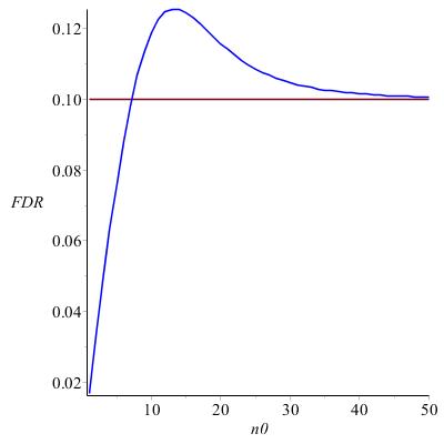
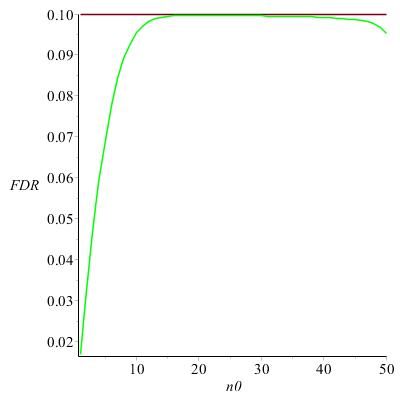
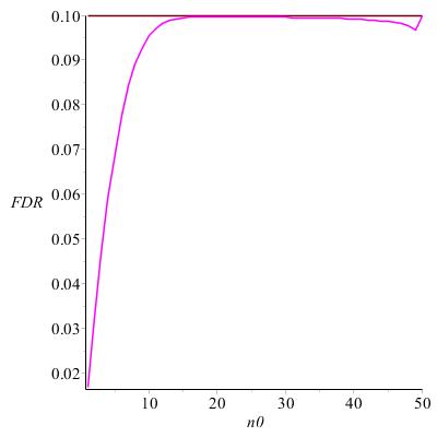
Figure 1: The FDR under Dirac uniform configuration, as function of $n_{0},\ 1\leqslant n_{0}\leqslant n$, of SU (blue line), SD (green line) and SD with improved first critical value (magenta line) for Dirac uniform configuration of the procedures based on the set of critical values $\beta_{i},\ i\leqslant n$ with $n=50,\ \alpha=0.1.$

As we can see from the Figure 1, the FDR of the SU test may be larger than prechosen level $\alpha$ in contrast to the SD test based on the same critical values $\beta_{i},i\leqslant n$. The next theorem gives an explanation in terms of the ENFR.

Theorem 23.

Let $(p_{i})_{i\in I_{0}}$ fulfil the reverse martingale dependence assumption (R) and $p_{j}=0$ whenever $j\in I_{1}$. For $f(n)=\frac{2\alpha(n+1)^{2}}{n+3}$ we get

• ${\mathbb{E}}\left[V(\tau_{SU})\right]\geqslant\frac{\alpha}{1-\alpha}(n_{1}+1)$ for all $n_{0}\geqslant f(n),$

• FDR${}_{\tau_{SU}}\geqslant\alpha$ for all $n_{0}\geqslant f(n)$.

Moreover, we have ”$>$” in (a) and (b) if $n_{0}>f(n)$.

In the concrete situation of Figure 1 we observe $f(50)=9.8$, which is visible in the first grafic.

5 The proofs and technical results

The proof of Lemma 3 is obvious.

Proof of Lemma 5.

(a) Firstly, consider the case $\{\beta_{i}:p_{i:n}>\beta_{i},\ i\leqslant n\}\neq\emptyset$ and define $j^{*}=\min\{i:p_{i:n}>\beta_{i},\ i\leqslant n\}.$ Then, we get $\sigma=\beta_{j^{*}}$ due to the definition of $\sigma$. This implies

$$\beta_{j^{*}}<p_{j^{*}:n}\text{\ and \ }\beta_{i}\geqslant p_{i:n}\text{ \ for \ all \ }i\leqslant j^{*}-1.$$

Consequently we get

$$p_{j^{*}-1}\leqslant\beta_{j^{*}-1}<\beta_{j^{*}}<p_{j^{*}:n},$$

which implies $R(\beta_{j^{*}-1})=R(\beta_{j^{*}})=j^{*}-1$. Due to (2.3) we get

$$j^{*}=\min\{i:\hat{\alpha}_{n}(\beta_{i})=\alpha,\ i\leqslant n\},$$

which completes the proof for this case. The case $\{\beta_{i}:p_{i:n}>\beta_{i},\ i\leqslant n\}=\emptyset$ is obvious since $\hat{\alpha}(t)=0$ if $\hat{F}_{n}(t)=1$.
The first statement of (b) is obvious and coincides with Remark 2. If there is any index $i\leqslant n$ with $R(\beta_{i})=i-1$, then $\hat{\alpha}_{n}(\sigma)=\alpha$ due to (2.2) and (a).
Otherwise we have $\hat{\alpha}_{n}(\beta_{i})<\alpha$ for all $i\leqslant n$ and $R(\sigma)=R(\beta_{n})=n$ holds. This implies $\hat{\alpha}_{n}(\sigma)=0.$ Consequently, we get $\hat{\alpha}_{n}(\sigma)=\alpha\mbox{$\mathbb{I}$}(R(\sigma)<n)$.
The part (c) is obvious.∎

Since $\tau_{SD}$ is not a stopping time w.r.t. $\mathcal{F}_{T}$ we will turn to the critical boundary $\sigma$ in order to apply Lemma 5.

Proof of Lemma 6 and Theorem 8.

Firstly´, note that we have $V(\sigma)=V(\tau_{SD})$, as well as $S(\sigma)=S(\tau_{SD})$. Due to Lemma 5 (b) we have $\hat{\alpha}_{n}(\sigma)=\alpha\mbox{$\mathbb{I}$}(R(\sigma)<n)$. Further, we obtain

$$(1-\hat{\alpha}_{n}(\sigma))(R(\sigma)+1)=M_{I_{0}}(\sigma)+\frac{S(\sigma)-n_{1}\sigma}{1-\sigma}+1$$ (5.1)

by (2.1) and (2.4) which is a fundamental equation connection between $\hat{\alpha}(\cdot)$ and $M_{I_{0}}(\cdot)$.

In case $S(\sigma)=n_{1}$ of Lemma 6 we have

$$(1-\alpha)V(\sigma)=M_{I_{0}}(\sigma)+\alpha(n_{1}+1)-\alpha(n+1)\mbox{$\mathbb{I}$}(V(\sigma)=n_{0}),$$ (5.2)

which implies the equivalence in Lemma 6.
Under the conditions of Theorem 8 we have ${\mathbb{E}}\left[M_{I_{0}}(\sigma)\right]\leqslant 0$ by the optional sampling Theorem of stopped super-martingales. Thus, the fact that $\frac{S(\sigma)-n_{1}\sigma}{1-\sigma}\leqslant S(\sigma)$ implies

$$(1-\alpha){\mathbb{E}}\left[V(\tau_{SD})\right]=(1-\alpha){\mathbb{E}}\left[V(\sigma)\right]\leqslant{\mathbb{E}}\left[M_{I_{0}}(\sigma)\right]+\alpha{\mathbb{E}}\left[S(\sigma)+1\right]\leqslant\alpha(n_{1}+1)$$ (5.3)

due to (5.1) and Remark 2. ∎

Proof of Lemma 9.

(a) Consider again the equality (5.2). If expectations are taken, the optional sampling theorem applies to $M_{I_{0}}(\sigma)$, which proves the result by Lemma 5 (a).
(b) Analogous to the case (a) we have

$$(1-\alpha)(V(\sigma)+S(\sigma)+1)+\alpha(n+1)\mbox{$\mathbb{I}$}(R(\sigma)=n)=M_{I_{0}}(\sigma)+M_{I_{1}}(\sigma)+1,$$ (5.4)

thereby $M_{I_{1}}(t)=\frac{\sum\limits_{i\in I_{1}}\mbox{$\mathbb{I}$}(p_{i}\leqslant t)-n_{1}t}{1-t}$ is a $\mathcal{F}_{t}^{T}-$martingale. Equality (5.4) implies

$$(1-\alpha){\mathbb{E}}\left[V(\sigma)+S(\sigma)\right]=\alpha-\alpha(n+1)P(R(\sigma)=n)$$ (5.5)

by taking the expectation ${\mathbb{E}}$ and applying the Optional Sampling Theorem. The equality ${\mathbb{E}}\left[S(\sigma)\right]=\frac{n_{1}}{n_{0}}{\mathbb{E}}\left[V(\sigma)\right]$ (which follows from the assumption that all p-values are identically distributed) completes the proof of part (b) of this lemma.
(c) The proof follows immediately from the observation that under martingale dependence the critical boundary value $\tau_{SD}$, and, consequently, $V(\tau_{SD})$, becomes maximal under assumptions of part (a) and minimal under assumptions of part (b). ∎

Remark 24.

1. The proof of the next Lemma 12 uses the technique which was proposed by Finner and Roters [9] for the proof of FDR-control of Benjamini and Hochberg test under PRDS.

2. As long as we are vconcerned with the super-martingale assumption (D1) we may assume w.l.o.g. that $\left(p_{i}\right)_{i\in I_{0}}$ are identically distributed and stochastically larger than $U(0,1)$, c.f Remark 7. These technical tools are only used for the subsequent proofs of Sections 2.2 - 2.4 in connection with PRDS. The reference to Remark 7 is not cited again in each step of the proofs.

Proof of Lemma 12.

Let us define $\beta_{0}=0$ for technical reasons and denote $(U_{j})_{j\leqslant n_{0}}:=(p_{i})_{i\in I_{0}}.$ Firstly, note that $\tau_{SD}=\beta_{R}$ holds obiously. Thereby, $R=R(\tau_{SD})$ is the number of rejections of the SD procedure with deterministic critical values $\beta_{i},\ i\leqslant n$. We obtain the following sequence of (in)equalities:

$${\mathbb{E}}\left[\frac{V(\tau_{SD})}{\tau_{SD}}\right]=\sum\limits_{j=1}^{n_{0}}{\mathbb{E}}\left[\frac{\mbox{$\mathbb{I}$}(U_{j}\leqslant\beta_{R})}{\beta_{R}}\right]$$ (5.6)

$$=\sum\limits_{j=1}^{n_{0}}\sum\limits_{i=1}^{n}{\mathbb{E}}\left[\frac{\mbox{$\mathbb{I}$}(U_{j}\leqslant\beta_{i})}{\beta_{i}}\mbox{$\mathbb{I}$}(\beta_{R}=\beta_{i})\right]$$ (5.7)

$$=\sum\limits_{j=1}^{n_{0}}\sum\limits_{i=1}^{n}{\mathbb{E}}\left[\frac{\mbox{$\mathbb{I}$}(U_{j}\leqslant\beta_{i})}{\beta_{i}}\left(\mbox{$\mathbb{I}$}(\beta_{R}\leqslant\beta_{i})-\mbox{$\mathbb{I}$}(\beta_{R}\leqslant\beta_{i-1})\right)\right]$$ (5.8)

$$=\sum\limits_{j=1}^{n_{0}}\sum\limits_{i=1}^{n}\frac{P(U_{j}\leqslant\beta_{i})}{\beta_{i}}{\mathbb{E}}\left[\frac{\mbox{$\mathbb{I}$}(U_{j}\leqslant\beta_{i})\left(\mbox{$\mathbb{I}$}(\beta_{R}\leqslant\beta_{i})-\mbox{$\mathbb{I}$}(\beta_{R}\leqslant\beta_{i-1})\right)}{P(U_{j}\leqslant\beta_{i})}\right]$$ (5.9)

$$\leqslant\sum\limits_{j=1}^{n_{0}}\sum\limits_{i=1}^{n}\left({\mathbb{E}}\left[\mbox{$\mathbb{I}$}(\beta_{R}(p)\leqslant\beta_{i})|U_{j}\leqslant\beta_{i}\right]-{\mathbb{E}}\left[\mbox{$\mathbb{I}$}(\beta_{R}(p)\leqslant\beta_{i-1})|U_{j}\leqslant\beta_{i}\right]\right)$$ (5.10)

$$\leqslant\sum\limits_{j=1}^{n_{0}}\sum\limits_{i=1}^{n}\left({\mathbb{E}}\left[\mbox{$\mathbb{I}$}(\beta_{R}\leqslant\beta_{i})|U_{j}\leqslant\beta_{i}\right]-E\left[\mbox{$\mathbb{I}$}(\beta_{R})\leqslant\beta_{i-1})|U_{j}\leqslant\beta_{i-1}\right]\right)$$ (5.11)

$$=\sum\limits_{j=1}^{n_{0}}{\mathbb{E}}\left[\mbox{$\mathbb{I}$}(\beta_{R}\leqslant\beta_{n})|U_{j}\leqslant\beta_{n}\right]=n_{0}.$$ (5.12)

The inequality in (5.10) is valid since $U_{1},...,U_{n_{0}}$ are stochastically greater than $U(0,1)$. The inequality in (5.11) holds because the function $x\mapsto\mbox{$\mathbb{I}$}(\beta_{R}(p)\leqslant\beta_{i-1}\mid U_{i}\leqslant x)$ is increasing in $x$ for all $i\in\{1,...,n_{0}\}$ and since $U_{1},...,U_{n_{0}}$ are assumed to be PRDS. Consequently, using the telescoping sum we obtain the first equality in (5.12). The proof is completed because $\beta_{R}(p)\leqslant\beta_{n}$ by definition of $\beta_{R}=\tau_{SD}.$ ∎

Proof of Theorem 11.

Combining Lemma 3, Theorem 8 and Lemma 12 yields the statement. ∎

To prove Theorem 14 we need the following technical result.

Lemma 25.

Under the assumptions of Theorem 14

$$E\left[\frac{M(\sigma)}{S(\sigma)+1}\right]\leqslant 0.$$

Proof of Lemma 25.

First, note that the process $\beta_{i}\mapsto S(\beta_{i})$ is always $\mathcal{F}_{T}^{f}$-measurable. If we put $M=M_{I_{0}}$ then

$$\begin{aligned} &{\mathbb{E}}\left[\frac{M(\sigma)}{S(\sigma)+1}\right]={\mathbb{E}}\left[\sum\limits_{i=1}^{n}\frac{M(\beta_{i})}{S(\beta_{i})+1}\mbox{$\mathbb{I}$}(\sigma=\beta_{i})\right]\\ &={\mathbb{E}}\left[\sum\limits_{i=1}^{n}\frac{M(\beta_{i})}{S(\beta_{i})+1}\left(\mbox{$\mathbb{I}$}(\sigma\leqslant\beta_{i})-\mbox{$\mathbb{I}$}(\sigma\leqslant\beta_{i-1})\right)\right]\\ &=\sum\limits_{i=1}^{n}\left({\mathbb{E}}\left[\frac{M(\beta_{i})}{S(\beta_{i})+1}\mbox{$\mathbb{I}$}(\sigma\leqslant\beta_{i})\right]-{\mathbb{E}}\left[{\mathbb{E}}\left[\frac{M(\beta_{i})}{S(\beta_{i})+1}\mbox{$\mathbb{I}$}(\sigma\leqslant\beta_{i-1})|\mathcal{F}_{\beta_{i-1}}^{f}\right]\right]\right).\end{aligned}$$ (5.13)

Since $\sigma$ is a $\mathcal{F}_{T}^{f}$-stopping time, $S(\beta_{i})$ is a measurable w.r.t. $\mathcal{F}_{\beta_{i-1}}^{f}$ and using martingale property ${\mathbb{E}}\left[M(\beta_{i})|\mathcal{F}_{\beta_{i-1}}^{f}\right]=M(\beta_{i-1})$ we get

$${\mathbb{E}}\left[{\mathbb{E}}\left[\frac{M(\beta_{i})}{S(\beta_{i})+1}\mbox{$\mathbb{I}$}(\sigma\leqslant\beta_{i-1})|\mathcal{F}_{\beta_{i-1}}^{f}\right]\right]={\mathbb{E}}\left[\frac{M(\beta_{i-1})}{S(\beta_{i})+1}\mbox{$\mathbb{I}$}(\sigma\leqslant\beta_{i-1})\right].$$

Define $\beta_{0}=0.$ Now, we can continue the chain of equalities (5.13) as follows.

$$\begin{aligned} &\sum\limits_{i=1}^{n}\left({\mathbb{E}}\left[\frac{M(\beta_{i})}{S(\beta_{i})+1}\mbox{$\mathbb{I}$}(\sigma\leqslant\beta_{i})\right]-{\mathbb{E}}\left[\frac{M(\beta_{i-1})}{S(\beta_{i-1})+1}\mbox{$\mathbb{I}$}(\sigma\leqslant\beta_{i-1})\right]\right)\\ &+\sum\limits_{i=1}^{n}\left({\mathbb{E}}\left[\frac{M(\beta_{i-1})}{S(\beta_{i-1})+1}\mbox{$\mathbb{I}$}(\sigma\leqslant\beta_{i-1})\right]-{\mathbb{E}}\left[\frac{M(\beta_{i-1})}{S(\beta_{i})+1}\mbox{$\mathbb{I}$}(\sigma\leqslant\beta_{i-1})\right]\right)\\ \end{aligned}$$ (5.14)

$$=\sum\limits_{i=1}^{n}\left({\mathbb{E}}\left[\frac{S(\beta_{i})-S(\beta_{i-1})}{(S(\beta_{i-1})+1)(S(\beta_{i}+1))}{\mathbb{E}}_{f}\left[M(\beta_{i-1})\mbox{$\mathbb{I}$}(\sigma\leqslant\beta_{i-1}))\right]\right]\right)$$ (5.15)

because the first term in (LABEL:firstsum) is equal to zero due to the telescoping sum since ${\mathbb{E}}\left[M(\beta_{n})\right]=0$. Now, we will show that

$${\mathbb{E}}\left[M(\beta_{i-1})\mbox{$\mathbb{I}$}(\sigma\leqslant\beta_{i-1}))\right]\leqslant 0$$ (5.16)

for all $i\leqslant n.$ Indeed, we have

$${\mathbb{E}}\left[M(\beta_{i-1})\mbox{$\mathbb{I}$}(\sigma\leqslant\beta_{i-1}))\right]=-{\mathbb{E}}\left[M(\beta_{i-1})\mbox{$\mathbb{I}$}(\sigma>\beta_{i-1}))\right].$$ (5.17)

Further, by the definition of $\sigma$ we know that $\hat{\alpha}_{n}(t)\leqslant\alpha$ for all $t\leqslant\sigma,\ t\in T$. Hence, due to (2.2) we get $\mbox{$\mathbb{I}$}(\sigma>\beta_{i-1}))=\prod\limits_{j=0}^{i-1}\mbox{$\mathbb{I}$}\left(R(\beta_{j})\geqslant j-1\right)$. On the other hand, we can conclude from the definition of the process $M_{I_{0}}$ that $\mbox{$\mathbb{I}$}\left(R(\beta_{j})\geqslant j-1\right)=\mbox{$\mathbb{I}$}\left(M(\beta_{j})\geqslant c(j)\right)$. Thereby, constants $c_{j},\ j\leqslant i-1,$ are defined as $c_{j}=\frac{j-1-S(\beta_{j})-n_{0}\beta_{j}}{1-\beta_{j}}.$ Consequently, (5.16) is equivalent to

$${\mathbb{E}}\left[M(\beta_{i-1})\prod\limits_{j=0}^{i-1}\mbox{$\mathbb{I}$}\left(M(\beta_{j})\geqslant c(j)\right))\right]\geqslant 0,$$ (5.18)

which follows immediately from the following Lemma 26 (by setting $X=M(\beta_{i-1})$ and $A=\prod\limits_{j=0}^{i-2}\mbox{$\mathbb{I}$}(M(\beta_{j})\geqslant c(j))$) and Lemma 27. ∎

Lemma 26.

Let $X$ be a random variable with ${\mathbb{E}}\left[X\right]=0,\ A$ be a measurable set and $c\in\mathbb{R}$ be some constant. The inequality ${\mathbb{E}}\left[\mbox{$\mathbb{I}$}_{A}X\right]\geqslant 0$ implies ${\mathbb{E}}\left[\mbox{$\mathbb{I}$}_{A}X\mbox{$\mathbb{I}$}(X>c)\right]\geqslant 0.$

Proof of Lemma 26.

The case $c\geqslant 0$ is obvious. If $c<0$ we get

$$0\leqslant{\mathbb{E}}\left[\mbox{$\mathbb{I}$}_{A}X\right]={\mathbb{E}}\left[\mbox{$\mathbb{I}$}_{A}X\mbox{$\mathbb{I}$}(X>c)\right]+{\mathbb{E}}\left[\mbox{$\mathbb{I}$}_{A}X\mbox{$\mathbb{I}$}(X\leqslant c)\right]\leqslant{\mathbb{E}}\left[\mbox{$\mathbb{I}$}_{A}X\mbox{$\mathbb{I}$}(X>c)\right],$$

which implies the proof of this lemma. ∎

Lemma 27.

Under the assumptions of Theorem 14 we have

$${\mathbb{E}}\left[M(\beta_{i-1})\prod\limits_{j=0}^{i-2}\mbox{$\mathbb{I}$}(M(\beta_{j})\geqslant c(j))\right]\geqslant 0\ \text{for}\ i\geqslant 2.$$ (5.19)

Proof of Lemma 27.

The proof is based on induction. Firstly, we define $k:=i-1$.
Let $k=2$ then (5.19) is equivalent to

$${\mathbb{E}}\left[M(\beta_{2})\mbox{$\mathbb{I}$}(M(\beta_{1})\geqslant c(1))\right]\geqslant 0,$$

which is true due to the following chain of equalities.

$$\begin{aligned} &{\mathbb{E}}\left[M(\beta_{2})\mbox{$\mathbb{I}$}(M(\beta_{1})\geqslant c(1))\right]={\mathbb{E}}\left[{\mathbb{E}}\left[M(\beta_{2})\mbox{$\mathbb{I}$}(M(\beta_{1})>c(1))\geqslant c(1))|\mathcal{F}^{f}_{\beta_{1}}\right]\right]\\ &={\mathbb{E}}\left[\mbox{$\mathbb{I}$}(M(\beta_{1}){\mathbb{E}}\left[M(\beta_{2})|\mathcal{F}^{f}_{\beta_{1}}\right]\right]={\mathbb{E}}\left[M(\beta_{1})\mbox{$\mathbb{I}$}(M(\beta_{1})\geqslant c(1))\right].\end{aligned}$$ (5.20)

The two last equalities in (5.20) are valid due to the measurability of $M(\beta_{1})$ w.r.t. $\mathcal{F}^{f}_{\beta_{1}}$ and martingale property ${\mathbb{E}}\left[M(\beta_{2})|\mathcal{F}^{f}_{\beta_{1}}\right]=M(\beta_{1}).$
Assume that

$${\mathbb{E}}\left[M(\beta_{k})\prod\limits_{j=0}^{k-1}\mbox{$\mathbb{I}$}(M(\beta_{j})\geqslant c(j))\right]\geqslant 0$$ (5.21)

holds for $k\geqslant 2.$ Then we prove that

$${\mathbb{E}}\left[M(\beta_{k+1})\prod\limits_{j=0}^{k}\mbox{$\mathbb{I}$}(M(\beta_{j})\geqslant c(j))\right]\geqslant 0$$

is also true. We have

$${\mathbb{E}}\left[M(\beta_{k+1})\prod\limits_{j=0}^{k}\mbox{$\mathbb{I}$}(M(\beta_{j})\geqslant c(j))\right]={\mathbb{E}}\left[{\mathbb{E}}\left[M(\beta_{k+1})\prod\limits_{j=0}^{k}\mbox{$\mathbb{I}$}(M(\beta_{j})\geqslant c(j))|\mathcal{F}^{f}_{\beta_{k}}\right]\right]$$

$$={\mathbb{E}}\left[M(\beta_{k})\prod\limits_{j=0}^{k}\mbox{$\mathbb{I}$}(M(\beta_{j})\geqslant c(j))\right]={\mathbb{E}}\left[\left(M(\beta_{k})\prod\limits_{j=0}^{k-1}\mbox{$\mathbb{I}$}(M(\beta_{j})\geqslant c(j))\right)\mbox{$\mathbb{I}$}(M(\beta_{k})\geqslant c(k))\right]\geqslant 0.$$

The last inequality follows from (5.21) and Lemma 26. ∎

Now, we are able to prove Theorem 14.

Proof of Theorem 14.

Let us remind (5.1), which implies

$$(1-\alpha)V(\sigma)\leqslant M_{I_{0}}(\sigma)+\alpha(S(\sigma)+1).$$ (5.22)

Dividing by $S(\sigma)+1$ yields

$$(1-\alpha)\frac{V(\sigma)}{S(\sigma)+1}\leqslant\frac{M_{I_{0}}(\sigma)}{S(\sigma)+1}+\alpha.$$

Taking the expectation ${\mathbb{E}}\left[\cdot\right]$ and using Lemma 25 deliver the result. ∎

To prove Lemma 15 we need the following technical result.

Lemma 28.

Let $(b_{i})_{i\in I_{0}}$ be some set of real numbers with $b_{i}\in[0,1],\ i\in I_{0}$. If p-values $(p_{i})_{i\leqslant n}$ are PRDS on $I_{0}$ then

$$P\left(\bigcap\limits_{i\in I_{0}}\{p_{i}>b_{i}\}\right)\geqslant\prod\limits_{i\in I_{0}}P\left(p_{i}>b_{i}\right).$$ (5.23)

Proof.

W.l.o.g. let us assume that $I_{0}=\{1,...,n\}$. For any other subset $I_{0}$ the proof works in the same way. First, we show the inequality

$${\mathbb{E}}\left[\prod\limits_{i=2}^{n}\mbox{$\mathbb{I}$}(p_{i}>b_{i})\mid p_{1}>b_{1}\right]\geqslant{\mathbb{E}}\left[\prod\limits_{i=2}^{n}\mbox{$\mathbb{I}$}(p_{i}>b_{i})\mid p_{1}\leqslant b_{1}\right].$$ (5.24)

To do this let $F$ denote the marginal distribution function of $p_{1}$. Define $f(u)={\mathbb{E}}\left[\prod\limits_{i=2}^{n}\mbox{$\mathbb{I}$}(p_{i}>b_{i})|p_{1}=u\right]$, then we have

$${\mathbb{E}}\left[\prod\limits_{i=2}^{n}\mbox{$\mathbb{I}$}(p_{i}>b_{i})\mbox{$\mathbb{I}$}(p_{1}>b_{1})\right]=\int\limits_{b_{1}}^{1}f(u)dF(u)$$

and

$${\mathbb{E}}\left[\prod\limits_{i=2}^{n}\mbox{$\mathbb{I}$}(p_{i}>b_{i})\mbox{$\mathbb{I}$}(p_{1}\leqslant b_{1})\right]=\int\limits_{0}^{p_{1}}f(u)dF(u).$$

Then (5.24) is equivalent to

$$\frac{\int\limits_{b_{1}}^{1}f(u)dF(u)}{1-F(b_{1})}\geqslant\frac{\int\limits_{0}^{b_{1}}f(u)dF(u)}{F(b_{1})}.$$ (5.25)

From the mean value theorem for Riemann-Stieltjes integrals we can deduce that there exist some values $\xi_{1}$ and $\xi_{2}$ with

$$\begin{aligned} &\xi_{1}=\frac{\int\limits_{b_{1}}^{1}f(u)dF(u)}{1-F(b_{1})},&\mbox{\ \ \ }&\inf\limits_{t\in(b_{1},1)}f(t)\leqslant\xi_{1}\leqslant\sup\limits_{t\in(b_{1},1)}f(t),\\ &\xi_{2}=\frac{\int\limits_{0}^{b_{1}}f(u)dF(u)}{F(b_{1})},&\mbox{\ \ \ }&\inf\limits_{t\in(0,b_{1})}f(t)\leqslant\xi_{2}\leqslant\sup\limits_{t\in(0,b_{1})}f(t).\end{aligned}$$ (5.26)

Since $f$ is an increasing function of $u$, (5.26) yields $\xi_{1}\geqslant\xi_{2},$ hence we get (5.25).
Further, we obtain

$$P(p_{1}>b_{1},p_{2}>b_{2},...,p_{n}>b_{n})={\mathbb{E}}\left[\prod\limits_{i=1}^{n}\mbox{$\mathbb{I}$}(p_{i}>b_{i})\right]$$ (5.27)

$$=P(p_{1}>b_{1}){\mathbb{E}}\left[\prod\limits_{i=2}^{n}\mbox{$\mathbb{I}$}(p_{i}>b_{i})\mid p_{1}>b_{1}\right]\geqslant P(p_{1}>b_{1}){\mathbb{E}}\left[\prod\limits_{i=2}^{n}\mbox{$\mathbb{I}$}(p_{i}>b_{i})\right]$$ (5.28)

$$=P(p_{1}>b_{1})P(\bigcap\limits_{i=2}^{n}(p_{i}>b_{i}))\geqslant...\geqslant\prod\limits_{i=1}^{n}P(p_{i}>b_{i}).$$ (5.29)

The inequality in (5.29) holds due to the PRDS-assumption since according to the law of total probability we have

$$\begin{aligned} &{\mathbb{E}}\left[\prod\limits_{i=2}^{n}\mbox{$\mathbb{I}$}(p_{i}>b_{i})\right]={\mathbb{E}}\left[\prod\limits_{i=2}^{n}\mbox{$\mathbb{I}$}(p_{i}>b_{i})\mid p_{1}>b_{1}\right]-\\ &P(p_{1}\leqslant b_{1})\underbrace{\left({\mathbb{E}}\left[\prod\limits_{i=2}^{n}\mbox{$\mathbb{I}$}(p_{i}>b_{i})\mid p_{1}>b_{1}\right]-{\mathbb{E}}\left[\prod\limits_{i=2}^{n}\mbox{$\mathbb{I}$}(p_{i}>b_{i})\mid p_{1}\leqslant b_{1}\right]\right)}_{\geqslant 0\text{ \ due \ to }(\ref{prdspqd})}.\end{aligned}$$ (5.30)

∎

For the two following proofs we define the p-values, which belong to the true null by $\left(U_{i}\right)_{i\in\{1,...,n_{0}\}}=\left(p_{j}\right)_{j\in I_{0}}$. Now, we are able to prove Lemma 15 by conditioning under the portion $f$ belonging to the false null.

Proof of Lemma 15.

We consider an arbitrary FDR-controlling SD procedure that uses critical values $\alpha_{i},i\leqslant n.$ Let us define $j^{*}:=\max\{i:f_{j}\leqslant 1-(1-\alpha)^{\frac{1}{n}}\text{\ for \ all \ }j\leqslant i\}$ and consider two possible cases.

• Let $j^{*}=0$. In this case we have under PRDS assumption

  $${\mathbb{E}}_{f}\left[\frac{V}{R}\mbox{$\mathbb{I}$}(V>0)\right]\leqslant{\mathbb{E}}_{f}\left[\mbox{$\mathbb{I}$}(V>0)\right]=P(U_{1:n_{0}}\leqslant 1-(1-\alpha)^{\frac{1}{n}})$$

  $$=1-P(\bigcap\limits_{i=1}^{n_{0}}\{U_{i}>1-(1-\alpha)^{\frac{1}{n}}\})\leqslant\alpha,$$

  where the last inequality is valid due to Lemma 28.

• Let $j^{*}>0$. Define the vector $f^{*}_{0}=(0,...,0,f_{j^{*}+1},...,f_{n_{1}}),$ where the $j^{*}$ first coordinates are replaced by $0.$ We get

  $${\mathbb{E}}_{f}\left[\frac{V}{R}\mbox{$\mathbb{I}$}(V>0)\right]\leqslant{\mathbb{E}}_{f}\left[\frac{V}{j^{*}+V}\right]={\mathbb{E}}_{f^{*}_{0}}\left[\frac{V(\tau_{SD})}{R(\tau_{SD})}\right]\leqslant\alpha.$$ (5.31)

  Thereby, $\tau_{SD}$ is the critical boundary value corresponding to the SD procedure with critical values $\alpha_{i},\ i\leqslant n$.

∎

Proof of Lemma 17.

Note that ${\mathbb{E}}\left[\frac{V}{R}\right]={\mathbb{E}}\left[\mbox{$\mathbb{I}$}(f_{1}\leqslant d_{1})\frac{V}{R}+\mbox{$\mathbb{I}$}(f_{1}>d_{1})\frac{V}{R}\right]$ is always valid and let us consider two different cases: (a) $f_{1}\leqslant d_{1}$, (b) $f_{1}>d_{1}$.
(a) Since $f_{1}$ will be rejected, the equality ${\mathbb{E}}_{f_{0}}\left[\frac{V}{R}\right]={\mathbb{E}}_{f}\left[\frac{V}{R}\right]$ holds. Therefore the statement of the lemma is proved for this case.
(b) If $f_{1}>d_{1}$ holds, we have due to the PRDS assumption that

$${\mathbb{E}}_{f}\left[\frac{V}{R}\mbox{$\mathbb{I}$}(V>0)\right] \leqslant{\mathbb{E}}_{f}\left[\mbox{$\mathbb{I}$}(V>0)\right]=P(U_{1:n_{0}}\leqslant d_{1})$$

$$\leqslant P(U_{1:n_{0}}\leqslant 1-\sqrt[n]{1-\alpha})\leqslant\alpha,\mbox{ \ \ \ }$$

where $U_{1:n_{0}}$ is the smallest true p-value. Hence, we get ${\mathbb{E}}_{f}\left[\frac{V}{R}\right]\leqslant\alpha$ for all possible vectors $f=(f_{1},...,f_{n_{1}})$. Further, ${\mathbb{E}}\left[\frac{V}{R}\right]={\mathbb{E}}\left[{\mathbb{E}}_{f}\left[\frac{V}{R}\right]\right],$ which completes the proof. ∎

Proof of Lemma 18.

The optional stopping theorem for reverse martingales implies

$${\mathbb{E}}\left[\frac{V(\tau)}{\tau}\right]\leqslant\frac{V(1)}{1}=n_{0}.$$ (5.32)

In the case of reverse martingales we have an equality. ∎

It is quite obvious that the variables (3.2) and (3.4) are stopping times and Lemma 18 can be applied.
The proof of Theorem 21 requires some preparations. Consider a wider class of rejection curves given by positive parameters $b$ and $\alpha,\ \delta\geqslant 0$ and

$$g(t)=\frac{tb}{\delta t+\alpha},\ 0\leqslant t\leqslant 1,\ b>\delta+\alpha.$$ (5.33)

Note that the condition $g(1)>1$ is necessary for proper SU tests with critical values

$$a_{i}:=g^{-1}\left(\frac{i}{n}\right)=\frac{\alpha i}{nb-i\delta}.$$ (5.34)

By the choice $b=\frac{n+1}{n}$ and $\delta=1-\alpha$ the coefficients $\beta_{i}$ are included. Thus we arrive at the following equation for the FDR of (5.34)

$$\text{FDR}={\mathbb{E}}\left[\frac{V}{R}\right]=\frac{\alpha}{nb}{\mathbb{E}}\left[\frac{V}{a_{R}}\right]+\frac{\delta}{nb}{\mathbb{E}}\left[V\right]$$ (5.35)

for each multiple test. In contrast to SD tests the term ${\mathbb{E}}\left[\frac{V}{a_{R}}\right]$ can be bounded under the R-super-martingale condition, cf. Heesen and Janssen [14].

Remark 29.

Consider SU tests for parameters $(\delta,b,\alpha)$ under R-super-martingale models with fixed portion $n_{1}<n$ of false p-values.

• The R-martingale models are least favourable for bounding ${\mathbb{E}}\left[\frac{V}{a_{R}}\right].$

• Consider two settings $\left(p_{i}\right)_{i\leqslant n}$ and $\left(q_{i}\right)_{i\leqslant n}$ of R-martingale models. If $p_{i}\leqslant q_{i}$ holds for all $i\in I_{1}$ then ${\mathbb{E}}_{p}\left[V\right]\leqslant{\mathbb{E}}_{q}\left[V\right]$ and $\text{FDR}_{p}\leqslant\text{FDR}_{q}$ holds.

• Under BIA with uniformly distributed p-values under the null, as well as under the reverse martingale dependence (R), we have:

  • The Dirac uniform configuration DU$(n_{1})$ is least favourable for ${\mathbb{E}}\left[V\right]$ and FDR.

  • Suppose that $\frac{\alpha}{b}$ or $\frac{\delta}{b}$ increases. Then the coefficients $a_{i}$ increase and the FDR and ${\mathbb{E}}\left[V\right]$ do not decrease.

Proof of Theorem 21.

(a) Proposition 4.1 of Heesen and Janssen [14] establishes the asymptotic lower bound:

$$\sup\limits_{\mathcal{P}_{BI(n)}}\text{FDR}(n,\delta_{n})\geqslant\min\limits_{i\leqslant n}\frac{na_{i}}{i}=\frac{n\alpha}{n+1-\delta_{n}}\rightarrow\alpha$$

as $n\rightarrow\infty.$ To obtain the upper bound we can first exclude all coefficients $\delta_{n}=0$, which correspond to a Benjamini and Hochberg test with level $\frac{n\alpha}{n+1}.$ Fix some value $\gamma$ with $\limsup\limits_{n\rightarrow\infty}\delta_{n}<\gamma<1-\alpha$ and introduce the rejection curve $g_{\gamma}(t)=\frac{t}{\gamma t+\alpha}.$ For all $\delta_{n}<\gamma$ the FDR$(n,\delta_{n})$ of the $a_{i}$’s can now be compared with the FDR of the SU test with critical values $g_{\gamma}^{-1}\left(\frac{i}{n}\right)$. By (5.35) and Remark (29) we have for each regime

$$\text{FDR}(n,\delta_{n})\leqslant\text{FDR}_{n}(g_{\gamma}^{-1})$$

using obvious notations. The worst case asymptotics is given by Theorem 5.1 of Heesen and Janssen [14]

$$\limsup\limits_{n\rightarrow\infty}\sup\limits_{\text{BI}(n)}\text{FDR}_{n}(g_{\gamma}^{-1})=K,$$

where

$$K=\sup\left\{\frac{x}{1-x}\frac{1-g_{\gamma}(x)}{g_{\gamma}(x)}:0<x\leqslant g_{\gamma}^{-1}(1)\right\}=\alpha.$$

(b) Similarly as above the FDR$(n,\delta_{n})$ is bounded below and above by the FDR of SU given by rejection curves. Choose constants $0<\gamma_{1}<\delta<\gamma_{2}<1-\alpha$ and $b>1$ and consider $\delta_{n}\in(\gamma_{1},\gamma_{2})$ and large $n$ with $\frac{n+1}{n}\leqslant b.$ Introduce $g_{\gamma_{2}}(t)=\frac{t}{\gamma_{2}t+\alpha}$ and $g_{\gamma_{1},b}(t)=\frac{tb}{\gamma_{1}t+\alpha}$. Again we have

$$\text{FDR}_{n}(g_{\gamma_{1},b})\leqslant\text{FDR}(n,\delta_{n})\leqslant\text{FDR}_{n}(g_{\gamma_{2}}).$$

Let $x(\gamma_{2})\in(0,1)$ denote the unique solution of the equation

$$g_{\gamma_{2}}(x)=(1-c)+xc.$$ (5.36)

If we repeat the proof of Proposition 5.1 of Heesen and Janssen [14] we have

$$\limsup\limits_{n\rightarrow\infty}\text{FDR}_{n}(g_{\gamma_{2}})=\sup\{\frac{x}{1-x}\frac{1-g_{\gamma_{2}}(x)}{g_{\gamma_{2}}(x)}:x(\gamma_{2})\leqslant x\leqslant g_{\gamma_{2}}^{-1}(1)\}$$

which is equal to $\frac{cx(\gamma_{2})}{(1-c)+cx(\gamma_{2})}.$ Similarly, a lower bound of (3.9) is $\frac{cx(\gamma_{1},b)}{(1-c)+cx(\gamma_{1},b)}$ with solution $x(\gamma_{1},b)\in(0,1)$ of (5.36). If now $\gamma_{1}\uparrow\delta,\ \gamma_{2}\downarrow\delta$ and $b\downarrow\delta,$ the bounds turn to the value $\frac{cx(\delta)}{1-c+cx(\delta)}$ given by the solution $x(\delta)\in(0,1)$ of (5.36). ∎

Proof of Theorem 23.

Define the process $\left(\tilde{M}(t)\right)_{t\in T}=\left(\frac{V(t)}{t}-n_{0}\right)_{t\in T},$ which is, obviously, a centered reverse martingale w.r.t $\mathcal{G}_{t}^{T}$ due to the reverse martingale assumption. Now, we remind that for the step-wise procedure using critical values $(\beta_{i})_{i\leqslant n}$ the following equality is valid by (5.2):

$$(1-\alpha)V(\tau_{SU})=\tilde{M}(\tau_{SU})\frac{\tau}{1-\tau}-\alpha(n+1)\mbox{$\mathbb{I}$}(V(\tau_{SU}=n_{0}))+\alpha(n_{1}+1)$$

under the Dirac distribution of ”false” p-values $(p_{i})_{i\in I_{1}}.$ Thus, we have to show

$${\mathbb{E}}\left[\tilde{M}(\tau_{SU})\frac{\tau_{SU}}{1-\tau_{SU}}\right]\geqslant\alpha(n+1)P(V(\tau_{SU}))\text{ \ for \ }n_{0}\geqslant f(n)$$

to prove the part (a). First note, that because of $V(\tau_{SU})=V(\tau_{SU}\vee\beta_{1})$ it is enough to prove the statement of this theorem for the reverse stopping time $\tilde{\tau}_{SU}=\tau_{SU}\vee\beta_{1}$, where $\tilde{\tau}_{SU}\in\{\beta_{1},...,\beta_{n}\}.$ Fix an $\varepsilon=\varepsilon(n)>0$ with $\beta_{n}+\varepsilon<1$ and define a fictive additional coefficient $\beta_{n+1}=\beta_{n}+\varepsilon.$ Then, we have

$${\mathbb{E}}\left[\tilde{M}(\tilde{\tau}_{SU})\frac{\tilde{\tau}_{SU}}{1-\tilde{\tau}_{SU}}\right]=\sum\limits_{i=1}^{n}{\mathbb{E}}\left[\tilde{M}(\beta_{i})\frac{\beta_{i}}{1-\beta_{i}}\mbox{$\mathbb{I}$}(\tilde{\tau}_{SU}=\beta_{i})\right]$$ (5.37)

$$=\sum\limits_{i=1}^{n}{\mathbb{E}}\left[\tilde{M}(\beta_{i})\frac{\beta_{i}}{1-\beta_{i}}\mbox{$\mathbb{I}$}(\tilde{\tau}_{SU}\geqslant\beta_{i})-\tilde{M}(\beta_{i})\frac{\beta_{i}}{1-\beta_{i}}\mbox{$\mathbb{I}$}(\tilde{\tau}_{SU}\geqslant\beta_{i+1})\right].$$ (5.38)

Consider the term ${\mathbb{E}}\left[\tilde{M}(\beta_{i})\frac{\beta_{i}}{1-\beta_{i}}\mbox{$\mathbb{I}$}(\tilde{\tau}_{SU}\geqslant\beta_{i+1})\right].$ Since $\tilde{\tau}_{SU}$ is a reverse stopping time w.r.t. filtration $\mathcal{G}_{t}^{T}$ the value $\mbox{$\mathbb{I}$}(\tilde{\tau}_{SU}\geqslant\beta_{i+1})$ is $\mathcal{G}_{\beta_{i+1}}-$measurable. Further, using the reverse martingale property of $\tilde{M}(t)$ we get

$${\mathbb{E}}\left[\tilde{M}(\beta_{i})\frac{\beta_{i}}{1-\beta_{i}}\mbox{$\mathbb{I}$}(\tilde{\tau}_{SU}\geqslant\beta_{i+1})\right] =\frac{\beta_{i}}{1-\beta_{i}}{\mathbb{E}}\left[\mbox{$\mathbb{I}$}(\tilde{\tau}_{SU}\geqslant\beta_{i+1}){\mathbb{E}}\left[\tilde{M}(\beta_{i})|\mathcal{G}_{\beta_{i+1}}\right]\right]$$

$$=\frac{\beta_{i}}{1-\beta_{i}}{\mathbb{E}}\left[\mbox{$\mathbb{I}$}(\tilde{\tau}_{SU}\geqslant\beta_{i+1})\tilde{M}(\beta_{i+1})\right].$$

Consequently, continuing the chain of equalities (5.37)-(5.38) we get

$$\begin{aligned} &{\mathbb{E}}\left[\tilde{M}(\tilde{\tau}_{SU})\frac{\tilde{\tau}_{SU}}{1-\tilde{\tau}_{SU}}\right]\\ &=\sum\limits_{i=1}^{n}\left(\frac{\beta_{i}}{1-\beta_{i}}{\mathbb{E}}\left[\tilde{M}(\beta_{i})\mbox{$\mathbb{I}$}(\tilde{\tau}_{SU}\geqslant\beta_{i})\right]-\frac{\beta_{i}}{1-\beta_{i}}{\mathbb{E}}\left[\tilde{M}(\beta_{i+1})\mbox{$\mathbb{I}$}(\tilde{\tau}_{SU}\geqslant\beta_{i+1})\right]\right)\\ \end{aligned}$$ (5.39)

$$\begin{aligned} &=\sum\limits_{i=1}^{n}\left(\frac{\beta_{i}}{1-\beta_{i}}{\mathbb{E}}\left[\tilde{M}(\beta_{i})\mbox{$\mathbb{I}$}(\tilde{\tau}_{SU}\geqslant\beta_{i})\right]-\frac{\beta_{i+1}}{1-\beta_{i+1}}{\mathbb{E}}\left[\tilde{M}(\beta_{i+1})\mbox{$\mathbb{I}$}(\tilde{\tau}_{SU}\geqslant\beta_{i+1})\right]\right)\\ &+\sum\limits_{i=1}^{n}\left(\left(\frac{\beta_{i+1}}{1-\beta_{i+1}}-\frac{\beta_{i}}{1-\beta_{i}}\right){\mathbb{E}}\left[\tilde{M}(\beta_{i+1})\mbox{$\mathbb{I}$}(\tilde{\tau}_{SU}\geqslant\beta_{i+1})\right]\right)\\ &=\sum\limits_{i=1}^{n}\left(\left(\frac{\beta_{i+1}}{1-\beta_{i+1}}-\frac{\beta_{i}}{1-\beta_{i}}\right){\mathbb{E}}\left[\tilde{M}(\beta_{i+1})\mbox{$\mathbb{I}$}(\tilde{\tau}_{SU}\geqslant\beta_{i+1})\right]\right).\end{aligned}$$ (5.40)

The first sum in (5.40) vanishes due to telescoping summation and the fact that ${\mathbb{E}}\left[\tilde{M}(\beta_{1})\right]=0$. Note also that ${\mathbb{E}}\left[\tilde{M}(\beta_{n+1})\mbox{$\mathbb{I}$}(\tilde{\tau}_{SU}\geqslant\beta_{n+1})\right]=0$ because $\mbox{$\mathbb{I}$}(\tilde{\tau}_{SU}\geqslant\beta_{n+1})=0$. Now, we have to show

$$\sum\limits_{i=1}^{n-1}B_{i}\geqslant\alpha(n+1)P(V(\tilde{\tau}_{SU})=n_{0})\text{ \ for \ }n_{0}\leqslant f(n).$$ (5.41)

where

$$B_{i}=\left(\frac{\beta_{i+1}}{1-\beta_{i+1}}-\frac{\beta_{i}}{1-\beta_{i}}\right){\mathbb{E}}\left[\tilde{M}(\beta_{i+1})\mbox{$\mathbb{I}$}(\tilde{\tau}_{SU}\geqslant\beta_{i+1})\right],\ i\leqslant n-1.$$

First, note that all $B_{i}$ are non-negative for all $i\leqslant n-1,$ due to Lemma 16. Moreover, note that

$$\tilde{\tau}_{SU}=\beta_{n}\iff\ V(\beta_{n})=n_{0}$$

under the Dirac distribution of $(p_{i})_{i\in I_{1}}$ and consider the last summand

$$B_{n-1}=\left(\frac{\beta_{n}}{1-\beta_{n}}-\frac{\beta_{n-1}}{1-\beta_{n-1}}\right){\mathbb{E}}\left[\tilde{M}(\beta_{n})\mbox{$\mathbb{I}$}(\tilde{\tau}_{SU}\geqslant\beta_{n})\right]$$

$$=\left(\frac{\beta_{n}}{1-\beta_{n}}-\frac{\beta_{n-1}}{1-\beta_{n-1}}\right){\mathbb{E}}\left[\left(\frac{n_{0}}{\beta_{n}}-n_{0}\right)\mbox{$\mathbb{I}$}(\tilde{\tau}_{SU}=\beta_{n})\right]$$

$$=\left(1-\frac{\beta_{n-1}}{1-\beta_{n-1}}\frac{1-\beta_{n}}{\beta_{n}}\right)n_{0}P\left(V(\tilde{\tau}_{SU})=n_{0}\right)$$

$$=\frac{n+3}{2(n+1)}n_{0}P\left(V(\tilde{\tau}_{SU})=n_{0}\right)\geqslant\alpha(n+1)P(V(\tilde{\tau}_{SU})=n_{0})$$

if $n_{0}\geqslant f(n)=\frac{2\alpha(n+1)^{2}}{n+3}.$ This completes the proof of part (a).
(b) The second part follows immediately from (a) and from the formula for FDR of SU procedure based on the set of critical values $(\beta_{i})_{i\leqslant n}$ under the reverse martingale model:

$$\text{FDR}=\frac{\alpha n_{0}}{n+1}+\frac{1-\alpha}{n+1}{\mathbb{E}}\left[V\right].$$

∎

Appendix. Examples of martingale models.

The family of (super-)martingales is a rich class of models which is briefly reviewed below. In this section we present a couple of examples. Further examples can be found in Heesen and Janssen [14] and Benditkis [1]. For convenience let us describe the model in this section by distributions $P$ on $[0,1]^{n},$ where the coordinates $(p_{1},...,p_{n})\in[0,1]^{n}$ represent p-values. We restrict ourselves to martingale models

$$\left([0,1]^{n},P,(\mathcal{F}_{t}^{T})_{t\in T}\right).$$ (5.42)

Let $\mathcal{M}_{I_{0},I_{1}}^{T}$ denote the set of martingale models $P$ on $[0,1]^{n}$ for fixed portion $I_{0}\neq\emptyset,\ I_{1}$ of $\{1,...,n\}$ and $\{0\}\subset T\subset[0,\eta]$ for some $0<\eta<1.$
Obviously, there is a one to one correspondence between martingales and reverse martingales via the transformation

$$\tilde{p}_{i}=1-p_{i},\ \tilde{T}=\{1-t:t\in T\},\mathcal{G}_{t}^{\tilde{T}}:=\sigma(\mbox{$\mathbb{I}$}(p_{i}\geqslant s),\ s\geqslant t,\ s,t\in\tilde{T})$$ (5.43)

of (5.42). Note also that $(p_{i})_{i\in I_{0}}$ follow special copula models if each $p_{i},\ i\in I_{0},$ is uniformly distributed on $(0,1).$
To warm up consider first some useful elementary examples which will be combined below.

Example 30.

• (Marshall and Olkin type dependence (see Marshall and Olkin [16])) Let $X_{1},...,X_{n}$ be i.i.d. continuous distributed real random variables and $Y$ be a continuously distributed real random variable independent of $X_{1},...,X_{n}.$ Consider $Z_{i}:=\min(X_{i},Y)$ and $\tilde{Z}_{i}:=\max(X_{i},Y)$ for $1\leqslant i\leqslant n$. The transformed true p-values $p_{i}:=H(Zi)$ and $\tilde{p}_{i}:=\tilde{H}(Zi),\ i=1,...,n$ fulfil the martingale property, reverse martingale property, respectively. Thereby, $H$ and $\tilde{H}$ are distribution functions of $Z_{i}$ and $\tilde{Z}_{i},\ i\leqslant n.$

• (Block models) Suppose that the index set

  $$\{1,...,n\}=\sum\limits_{j=1}^{k}(I_{0,j}+I_{1,j})$$

  splits in $k$ disjoint portions of $I_{0,j}$ the true and $I_{1,j}$ false null. Let $U_{1},...,U_{k}$ denote i.i.d uniformly distributed random variables on $(0,1).$ Suppose that
  $\left((U_{1},(p_{i})_{i\in I_{1,1}}),(U_{2},(p_{i})_{i\in I_{1,2}}),...,(U_{k},(p_{i})_{i\in I_{1,k}})\right))$ are independent martingale models of dimension $|I_{1,j}|+1$ for $j\leqslant k$. The $U$’s can be duplicated by the definition

  $$p_{i}=U_{j}\ \text{if}\ i\in I_{0,j},\ I_{0}=\sum\limits_{j=1}^{k}I_{0,j},$$

  and we arrive at a martingale model where $\left(p_{i}\right)_{i\in\sum\limits_{j=1}^{k}I_{1,j}}$ are already defined.

Let us summarize further results.

Example 31.

• $M_{I_{0},I_{1}}^{T}$ is closed under convex combinations.

• New martingale models can be produced by stopped martingales via stopping times and the optional switching device, see Heesen and Janssen [14], p.685.

• (Martingales and financial models) Let $T\subset[0,\eta],\ \eta<1$ be a set with $0\in T$. Introduce the price process

  $$X_{t}:[0,1)^{n}\rightarrow[0,\infty),\ X_{t}(p_{1},...,p_{n})=\sum\limits_{i\in I_{0}}\left(\frac{\mbox{$\mathbb{I}$}(p_{i}\leqslant t)-t}{1-t}+K\right),\ t\in T$$

  on $T$ for some constant $K\geqslant\max(\frac{s}{1-s}),\ s\in T.$ Then the process $t\mapsto X_{t}$ can be viewed as a discounted price process for time points $t\in T.$ The existence of martingale measures for $\left(X_{t},\mathcal{F}_{t}\right)_{t\in T}$ on the domain $[0,1]^{n}$ is well studied in mathematical finances, see Shiryaev (1999). When the parameter set $T$ is finite it turns out that the space of probability measures on $[0,1]^{n}$, making that process to be a martingale, is of infinite dimension.

• (Super-martingales) It is well known that the process

  $$\sum\limits_{i\in I_{0}}\left(\frac{\mbox{$\mathbb{I}$}(p_{i}\leqslant t)-t}{1-t}\right)=M_{t}+A_{t},\ t\in T$$ (5.44)

  admits a Doob-Meyer decomposition given by a $(\mathcal{F}_{t})_{t\in T}$ martingale $t\mapsto M_{t}$ and a compensator $t\mapsto A_{t}$ which is predictable with $A_{t}=0.$ Note that (5.44) is a supermartingale if $t\mapsto A_{t}$ is non-increasing.