Optical chirality in gyrotropic media: symmetry approach

Abstract

We discuss optical chirality in different types of gyrotropic media. Our analysis is based on the formalism of nongeometric symmetries of Maxwell’s equations in vacuum generalized to material media with given constituent relations. This approach enables us to derive directly conservation laws related to the nongeometric symmetries. For isotropic chiral media, we demonstrate that likewise free electromagnetic field, both duality and helicity generators belong to the basis set of nongeometric symmetries that guarantees the conservation of optical chirality. In gyrotropic crystals, which exhibit natural optical activity, the situation is quite different from the case of isotropic media. For light propagating along certain crystallographic direction, there arise two distinct cases, i. e., (1) the duality is broken but the helicity is preserved, or (2) only the duality symmetry survives. We show that the existence of one of these symmetries (duality or helicity) is enough to define optical chirality. In addition, we present examples of low-symmetry media, where optical chirality can not be defined.

I Introduction

The notion of chirality, the term originally coined by Lord Kelvin for any object which cannot be superimposed onto its mirror image Kelvin (1904), is perhaps one of the most fundamental concepts in nature ranging from particle physics to biology Dreiling and Gay (2014). After the discovery of a new conservation law for Maxwell’s equations in vacuum by Lipkin Lipkin (1964), it was realized that not only material objects but also fields can be characterized by certain chirality Morgan (1964); Kibble (1965). In particular, we can construct the conserving pseudoscalar for free electromagnetic field

$$C_{\chi}=\frac{1}{2}\int d^{3}r\left(\varepsilon_{0}\bm{E}\cdot\bm{\nabla}\times\bm{E}+\mu_{0}^{-1}\bm{B}\cdot\bm{\nabla}\times\bm{B}\right),$$ (1)

which is even under time-reversal ($T$) and odd under spatial inversion ($P$) transformations. These symmetry properties are consistent with definition of true chirality proposed by Barron Barron (1986, 2004), who stressed that we should distinguish it from false chirality with broken $T$-symmetry. In this respect, this quantity is eligible to be called optical chirality, which was originally coined zilch by Lipkin Lipkin (1964).

Later it was realized that besides classical conservation laws arising from the invariance under the space-time Poincaré group, free electromagnetic field is invariant under the eight-dimensional Lie algebra of nongeometric symmetry transformations. This algebra results in an infinite number of integro-differential conservation laws, which include zilch as a particular case Fushchich and Nikitin (1987). Together with the approach based on the nongeometric symmetries Fushchich and Nikitin (1987), these conservation laws were studied by means of the Lie theory and the Noether theorem Krivskii and Simulik (1989a, b); Ibragimov (2008); Cameron and Barnett (2012); Bliokh et al. (2013); Cameron (2014), by using the analogy between Maxwell’s and Dirac equations Barnett (2014), and through the gauge symmetry Philbin (2013).

For free electromagnetic field, it was demonstrated that the existence of the duality symmetry for Maxwell’s equations, i.e. the linear transformation that mixes electric and magnetic fields, engenders automatically the preservation of optical helicity, i.e. the projection of total angular momentum on the direction of linear momentum Calkin (1965); Zwanziger (1968); Drummond (1999, 2006).

The renewed interest to optical chirality has been stimulated through interdisciplinary studies in molecules and metamaterials Tang and Cohen (2010); Hendry et al. (2010); Tang and Cohen (2011); Hendry et al. (2012); Kamenetskii et al. (2013); Tomita et al. (2014). Notable progress in the field of optical angular momentum is also relevant to this directions Yao and Padgett (2011); Bliokh and Nori (2015). The relationship between optical chirality, helicity, and spin angular momentum of light was discussed in a number of papers Afanasiev and Stepanovsky (1996); Bliokh and Nori (2011); Coles and Andrews (2012); Cameron et al. (2012); Barnett et al. (2012); Bliokh et al. (2014a, b, 2015, 2016). A recent review on the general space-time symmetries of the Maxwell’s equations can be found in Dressel et al. (2015).

For electromagnetic field in media, the problem of optical chirality has been considered in Refs. Philbin (2013); Ragusa (1994, 1996). In dispersive media, the generalization of Lipkin’s zilch was established by Philbin Philbin (2013) by means of the Noether’s theorem applied to the specific gauge transformation of the magnetic vector potential. In isotropic chiral media, first order electromagnetic conservation laws were heuristically constructed by Ragusa in the relativistically noncovariant Ragusa (1994) and covariant forms Ragusa (1996).

The purpose of this paper is to develop a systematic approach to the optical chirality in gyrotropic media. To provide a theoretical basis for our treatment, we invoke the formalism of nongeometric symmetries in vacuum Fushchich and Nikitin (1987), and generalize it to media taking heed of the corresponding constituent equations. The key idea is to find the invariance algebra of nongeometric symmetries in media and to investigate whether the basis set of this algebra includes the transformations of duality and helicity.

At first, we analyze nongeometric symmetries in isotropic chiral media. Likewise electromagnetic field in vacuum Calkin (1965); Zwanziger (1968), isotropic chiral medium is self-dual, which automatically means that helicty is preserved Fernandez-Corbaton and Molina-Terriza (2013). However, as we explicitly show, in chiral media, the original eight-dimensional invariance algebra of free electromagnetic field is broken down to its four-dimensional subalgebra due to lack of the inversion symmetry. Duality and helicity are two essential generators of this subalgebra. For spatially nonuniform chiral medium, we find that the actual expression for optical chirality depends on the choice of constituent relations, in order to guarantee continuity of the chirality flow.

Next, we consider optical chirality in gyrotropic crystals, where surrounding symmetry is more restrictive, and, globally, neither duality nor helicity symmetry transformations are allowed. Although these symmetries can survive along the principal crystalline axes, the equivalence between duality and helicity, that holds in isotropic media, is lost. We find that in crystals with gyrotropic birefrigence both duality and helicity operations are allowed along the principal axis. Crystals possessing natural optical activity and belonging to the point groups $C_{n}$ or $C_{nv}$ ($n\geq 3$) provide an example, where helicity is preserved along the principal axis Fernandez-Corbaton (2013), while the duality symmetry is broken. The opposite situation is realized in achiral materials with natural optical activity, where the duality symmetry along the principal axis is preserved without helicity. The existence of either duality or helicity transformations along a certain direction leads to the conservations law for optical chirality, which is consistent with underlying symmetries.

In concluding remarks, we consider low-dimensional crystals, where we encounter the invariance algebra with neither preserved duality nor preserved helicity, which makes optical chirality ill defined.

II Free electromagnetic field

We begin with a brief review of the latest developments in symmetry analysis of the electromagnetic field in vacuum. We give a pedagogical introduction in the method of nongeometrical symmetries, which is generalized in the subsequent sections to electromagnetic field in media.

The discovery of a conservation law in Eq. (1) stimulated the discussion of the related ‘hidden’ symmetries for the electromagnetic field. Historically, it had been established shortly after the formulation of electrodynamics that the Maxwell’s equations in free space

$$\bm{\nabla}\times\bm{E}=-\partial_{t}\bm{B},\qquad \bm{\nabla}\times\bm{B}=\partial_{t}\bm{E},$$ (2)

$$\bm{\nabla}\cdot\bm{E}=0,\qquad \bm{\nabla}\cdot\bm{B}=0,$$ (3)

(in this section we use $c=1$ and $\hbar=1$) remain invariant under the duality transformation

$$\bm{E} \to\bm{E}\cos\theta+\bm{B}\sin\theta,$$ (4)

$$\bm{B} \to-\bm{E}\sin\theta+\bm{B}\cos\theta,$$ (5)

which can be viewed as ‘rotation’ in the pseudo-space of $\bm{E}$ and $\bm{B}$ vectors (for a review and historical background, see Refs. Cameron and Barnett (2012); Bliokh et al. (2013)).

In contrast to the Maxwell’s equations, standard Lagrangian formulation of electrodynamics is not symmetric under the duality transformation, and, to mitigate this obstacle, a duality symmetric form of the Lagrangian density was proposed Cameron and Barnett (2012); Bliokh et al. (2013). The duality symmetric form, on the basis of the Noether theorem, ties up the transformation in Eqs. (4, 5) with conservation of optical helicity

$$C_{\mathrm{hel}}=\frac{1}{2}\int d^{3}r\left(\bm{A}\cdot\bm{\nabla}\times\bm{A}+\bm{C}\cdot\bm{\nabla}\times\bm{C}\right),$$ (6)

written in terms of magnetic ($\bm{A}$) and electric ($\bm{C}$) vector potentials, which are determined by $\bm{E}=-\bm{\nabla}\times\bm{C}=-\partial_{t}\bm{A}$ and $\bm{B}=\bm{\nabla}\times\bm{A}$, and satisfy the symmetry transformation in Eqs. (4, 5).

With respect to the optical helicity, Lipkin’s zilch in Eq. (1) can be regarded as the next order term in the infinite hierarchy of higher order conserving zilches Kibble (1965); Cameron et al. (2012). Although being different form optical helicity in general, for monochromatic fields, Lipkin’s zilch becomes proportional to the helicity. Both quantities are determined by the difference between left and right polarized photon numbers Bliokh and Nori (2011); Coles and Andrews (2012). Tang and Cohen proposed to use Lipkin’s $00$-zilch as a measure of optical chirality in light-matter interactions Tang and Cohen (2010, 2011).

Different approach to zilch conservation laws has been developed in Refs. Krivskii and Simulik (1989a, b); Ibragimov (2008) on the basis of the Lie-Noether analysis. Recently, Philbin explicitly demonstrated that zilch conservation can be obtained from the standard electromagnetic Lagrangian $L=(E^{2}-B^{2})/2$ by applying a specific ‘hidden’ gauge symmetry transformation of the magnetic vector potential, $\bm{A}\to\bm{A}+\eta\bm{\nabla}\times\partial_{t}\bm{A}$, with infinitesimal parameter $\eta$ Philbin (2013), similar to Calkin’s original arguments Calkin (1965).

Another powerful tool, different form the Lagrangian-Noether approach, that we used throughout this paper, is a method of the nongeometric symmetries developed by Fushchich and Nikitin Fushchich and Nikitin (1987). The advantage of this method is that it is solely based on the analysis of the equations of motion and, therefore, does not rely on any ambiguity in specific gauge choice or Lagrangian representation. This fact makes it possible to generalize this approach to Maxwell’s equations in media with given constituent relations.

For the symmetry analysis, it is essential to find convenient representation of the Maxwell’s equations. We use Silberstein-Bateman form, which is convenient to work in the momentum space. The transformation to the momentum space is reached by

$$\bm{E}(t,\bm{r}) =\frac{1}{(2\pi)^{3/2}}\int d^{3}p\,e^{i\bm{p}\cdot\bm{r}}\bm{E}(t,\bm{p}),$$ (7)

$$\bm{B}(t,\bm{r}) =\frac{1}{(2\pi)^{3/2}}\int d^{3}p\,e^{i\bm{p}\cdot\bm{r}}\bm{B}(t,\bm{p}).$$ (8)

In the Silberstein-Bateman representation, the first pair of the Maxwell’s equations in Eq. (2) is expressed in terms of a Shroedinger-like equation for a six-component vector column $\phi(t,\bm{p})=(\bm{E},\bm{B})^{T}$

$$i\frac{\partial\phi(t,\bm{p})}{\partial t}=\mathcal{H}\phi(t,\bm{p}),$$ (9)

where $\mathcal{H}$ is the Hermitian matrix given by

$$\mathcal{H}=-\sigma_{2}\otimes(\hat{\bm{S}}\cdot\bm{p})=\begin{pmatrix}0&i(\hat{\bm{S}}\cdot\bm{p})\\ -i(\hat{\bm{S}}\cdot\bm{p})&0\end{pmatrix},$$ (10)

which can be considered as an analogue of the quantum-mechanical Hamiltonian. Here, we introduced $3\times 3$ spin matrices $\hat{S}_{\alpha}$ with matrix elements $(\hat{S}_{\alpha})_{\beta\gamma}=-i\epsilon_{\alpha\beta\gamma}$, where $\epsilon_{\alpha\beta\gamma}$ is the Levi-Civita symbol, $\otimes$ means the Cartesian product, and $\sigma_{\mu}$ ($\mu=1,2,3$) are $2\times 2$ Pauli matrices. In what follows, we hold the following notations. The ‘hat’ is used to distinguish $3\times 3$ matrices. Calligraphic style is reserved for the $6\times 6$ matrices. $\sigma_{0}$ and $\hat{I}$ denote two- and three-dimensional unit matrices, and Greek indices run over the three dimensional space.

The second pair of Maxwell’s equations (3) is equivalent to the additional constrain imposed on $\phi(t,\bm{p})$ Fushchich and Nikitin (1987)

$$\mathcal{L}\phi(t,\bm{p})=0,\qquad{\cal L}=p^{2}-(\bm{\mathcal{S}}\cdot\bm{p})^{2},$$ (11)

where $\bm{\mathcal{S}}\equiv\sigma_{0}\otimes\hat{\bm{S}}$, which accounts for the transversal character of the electromagnetic field. For real $\phi(t,\bm{p})$, one should also require $\phi^{*}(t,\bm{p})=\phi(t,-\bm{p})$.

Now let us find all the transformations in the $\bm{p}$-space given by matrices $\mathcal{Q}_{A}(\bm{p})$ that transform a solution of the Maxwell’s equations $\phi(t,\bm{p})$ into another solution $\phi^{\prime}(t,\bm{p})=\mathcal{Q}_{A}(\bm{p})\phi(t,\bm{p})$. Following Ref. Fushchich and Nikitin (1987), we will call $\mathcal{Q}_{A}(\bm{p})$ nongeometric symmetry transformations. The total number of such $\mathcal{Q}_{A}(\bm{p})$ is given in the theorem, which claims that the Maxwell’s equations in vacuum are invariant under the eight-dimensional Lie algebra

$$\mathcal{Q}_{1} =\sigma_{3}\otimes(\hat{\bm{S}}\cdot\tilde{\bm{p}})\hat{D},\qquad \mathcal{Q}_{2} =i\sigma_{2}\otimes\hat{I},$$ (12)

$$\mathcal{Q}_{3} =-\sigma_{1}\otimes(\hat{\bm{S}}\cdot\tilde{\bm{p}})\hat{D},\qquad \mathcal{Q}_{4} =-\sigma_{1}\otimes\hat{D},$$ (13)

$$\mathcal{Q}_{5} =\sigma_{0}\otimes(\hat{\bm{S}}\cdot\tilde{\bm{p}}),\qquad \mathcal{Q}_{6} =-\sigma_{3}\otimes\hat{D},$$ (14)

$$\mathcal{Q}_{7} =\sigma_{0}\otimes\hat{I},\qquad \mathcal{Q}_{8} =i\sigma_{2}\otimes(\hat{\bm{S}}\cdot\tilde{\bm{p}}),$$ (15)

where $\tilde{\bm{p}}=\bm{p}/p$, $\hat{D}=\hat{D}_{0}+\hat{D}_{1}$ with $(\hat{D}_{0})_{\alpha\beta}=(\delta-f)p_{\alpha}p_{\beta}/(p^{2}\delta)$ and

$$\hat{D}_{1}=\frac{1}{\delta}\left(\begin{array}[]{ccc}f-2p_{2}^{2}p_{3}^{2}&p_{1}p_{2}p_{3}^{2}&p_{1}p_{3}p_{2}^{2}\\ p_{1}p_{2}p_{3}^{2}&f-2p_{1}^{2}p_{3}^{2}&p_{2}p_{3}p_{1}^{2}\\ p_{1}p_{3}p_{2}^{2}&p_{2}p_{3}p_{1}^{2}&f-2p_{1}^{2}p_{2}^{2}\end{array}\right),$$ (16)

where $f=p_{1}^{2}p_{2}^{2}+p_{1}^{2}p_{3}^{2}+p_{2}^{2}p_{3}^{2}$ and $\delta=[p_{1}^{4}(p_{2}^{2}-p_{3}^{2})^{2}+p_{2}^{2}p_{3}^{2}(p_{1}^{2}-p_{2}^{2})(p_{1}^{2}-p_{3}^{2})]^{1/2}$. The basis elements form the algebra, which is isomorphic to the Lie algebra of the group $U(2)\otimes U(2)$ Fushchich and Nikitin (1987).

All the basis elements in Eqs. (12)–(15) commute with $\mathcal{H}$ in Eq. (10) and act as generators for the continuous symmetry transformations

$$\phi(t,\bm{p})\to\exp(\mathcal{Q}_{A}\theta_{A})\phi(t,\bm{p}),$$ (17)

where $\theta_{A}$ are real parameters.

Analogy with quantum mechanics suggests that one can find conserving quantities related to the symmetry transformations $\mathcal{Q}_{A}$, which can be conveniently formulated in terms of bilinear forms

$$\left\langle\mathcal{Q}_{A}\right\rangle=\frac{1}{2}\int d^{3}p\,\phi^{{\dagger}}(t,\bm{p})\,\mathcal{M}\mathcal{Q}_{A}\,\phi(t,\bm{p}),$$ (18)

where $\mathcal{M}$ is any operator commutative with $\mathcal{H}$.

Some symmetry transformations in Eqs. (12)–(15) have transparent physical interpretations. For example, $\mathcal{Q}_{7}$ is the identity transformation. The corresponding conserving quantity is the electromagnetic energy

$$\left\langle\mathcal{Q}_{7}\right\rangle=\frac{1}{2}\int d^{3}p\phi^{{\dagger}}(t,\bm{p})\mathcal{Q}_{7}\phi(t,\bm{p})=\frac{1}{2}\int d^{3}p\left(E^{2}+B^{2}\right).$$ (19)

Duality transformation in Eqs. (4, 5) also belongs to the class on nongeometric symmetries. This symmetry is generated by $\mathcal{Q}_{2}$, in accordance with Eq. (17).

Electromagnetic chirality can be expressed as a conserving quantity that corresponds to the operator $p\mathcal{Q}_{5}$. Indeed, the expression

$$C_{\chi}=\frac{1}{2}\int d^{3}p\,\phi^{{\dagger}}(t,\bm{p})\,(\bm{\mathcal{S}}\cdot\bm{p})\,\phi(t,\bm{p}),$$ (20)

is transformed into Eq. (1) in the real space. In what follows, we would refer $\mathcal{Q}_{5}$ as a helicity operator, since electromagnetic helicity in Eq. (6) can be also expressed in terms of a bilinear form containing this operator acting in the space $(\bm{A},\bm{C})$.

By noting that $p\mathcal{Q}_{5}\mathcal{Q}_{2}=-i\mathcal{H}=\partial_{t}$, we can find an alternative form of the optical chirality expressed via the duality operator

$$C_{\chi}=-\frac{i}{2}\int d^{3}p\,\phi^{\dagger}(t,\bm{p})\,{\cal Q}_{2}\,\partial_{t}\phi(t,\bm{p}).$$ (21)

However, as we show in the next sections, the identity above between $\mathcal{Q}_{5}$, $\mathcal{Q}_{2}$, and $\mathcal{H}$ does not necessary hold in crystals, where it is possible that either $\mathcal{Q}_{2}$ or $\mathcal{Q}_{5}$ is allowed symmetry along certain crystallographic direction, but not both simultaneously.

Using the ambiguity in the choice of $\mathcal{M}$ in Eq. (18), we can identify the hierarchy of higher-rank conserving zilches, which contain high-order derivatives of electromagnetic fields. Substituting ${\cal M}=(-1)^{n+m}p^{2n}{\cal H}^{2m+1}$ into Eq. (21) (apparently, it commutes with $\mathcal{H}$), we obtain the following conserving quantities

$$C_{\chi}^{(m,n)}=\frac{1}{2}\int d^{3}r\left(\bm{B}\cdot\nabla^{2n}\partial_{t}^{2m+1}\bm{E}-\bm{E}\cdot\nabla^{2n}\partial_{t}^{2m+1}\bm{B}\right),$$ (22)

which were found previously by another methods (see e. g. Refs. Drummond (1999, 2006); Philbin (2013)).

III General formalism in media

The formalism of nongeometric symmetries can be generalized to Maxwell’s equations in medium, where symmetry of constituent relations imposes additional constrains on the form of conservation laws. In general, this leads to the reduction of original eight-dimensional invariance algebra $A_{8}$ to smaller number of elements. In this section, we analyze the situation when electromagnetic field propagates in time-independent dielectric medium. We show that, basically, $A_{8}$ shrinks to one of its commutative subalgebras $A_{4}$ with four basis elements. In the subsequent sections, we demonstrate that this situation is common for isotropic chiral media as far as for chiral gyrotropic crystals when light spreads along the principal symmetry direction. It should be mentioned that the existence of $A_{4}$ symmetry does not guarantee the conservation of optical chirality, as we discuss at the end of this section.

On a macroscopic level, the Maxwell’s equations in dielectric media can be expressed in the following form

$$\bm{\nabla}\times\bm{E}=-\partial_{t}\bm{B},\qquad \bm{\nabla}\times\bm{H}=\partial_{t}\bm{D},$$ (23)

$$\bm{\nabla}\cdot\bm{D}=0,\qquad \bm{\nabla}\cdot\bm{B}=0,$$ (24)

which should be accompanied by constituent relations. In what follows, we consider the following form of constituent relations

$$\left(\begin{array}[]{c}\bm{D}(t,\bm{p})\\ \bm{B}(t,\bm{p})\end{array}\right)=\mathcal{A}(\bm{p})\left(\begin{array}[]{c}\bm{E}(t,\bm{p})\\ \bm{H}(t,\bm{p})\end{array}\right),$$ (25)

where the momentum representation is used. The matrix $\mathcal{A}(\bm{p})$ is supposed to be time-independent and determined by the properties of medium.

For symmetry analysis in medium, it is convenient to introduce Silberstein-Bateman vector $\psi(t,\bm{p})=(\bm{D},\bm{B})^{T}$. In this case, the first pair of the Maxwell’s equations is written as

$${\cal L}^{(\mathcal{A})}\psi=0,\qquad{\cal L}^{(\mathcal{A})}=i\partial_{t}-{\cal H}^{(\mathcal{A})},$$ (26)

where

$${\cal H}^{(\mathcal{A})}=-\sigma_{2}\otimes(\hat{\bm{S}}\cdot\bm{p})\,\mathcal{A}^{-1},$$ (27)

and the constraint on $\psi(t,\bm{p})$ imposed by the second pair of Maxwell’s equations is the same as in Eq. (11).

For a common situation when constituent relations do not mix up electric and magnetic fields, Eq. (27) is reduced to the following expression

$${\cal H}^{(\mathcal{A})}=\begin{pmatrix}0&i(\hat{\bm{S}}\cdot\bm{p})\hat{\mu}^{-1}(\bm{p})\\ -i(\hat{\bm{S}}\cdot\bm{p})\hat{\varepsilon}^{-1}(\bm{p})&0\end{pmatrix},$$ (28)

where $\hat{\varepsilon}^{-1}(\bm{p})$ and $\hat{\mu}^{-1}(\bm{p})$ are inverse permittivity and permeability tensors.

III.1 Nongeometric symmetries

In general, it may be a tedious problem to find symmetry transformations for the Maxwell’s equations in medium. However, the task is alleviated along the directions where transverse electromagnetic waves can propagate. Mathematically, it corresponds to $\mathcal{A}(\bm{p})$ being commutative with $\mathcal{L}$ in Eq. (11) along such directions. In this case, to identify possible symmetry transformations we apply a transformation $\bar{\psi}=\mathcal{N}^{-1}\psi$ to the basis, where $\mathcal{H}^{(\mathcal{A})}$ and $\mathcal{L}$ are both diagonal

$$\bar{{\cal H}}^{({\cal A})} = \mathcal{N}^{-1}{\cal H}^{({\cal A})}\mathcal{N}=\mathop{\mathrm{diag}}\nolimits(\omega_{1},\omega_{2},0,\omega_{4},\omega_{5},0),$$ (29)

$$\bar{{\cal L}} = \mathcal{N}^{-1}{\cal L}\mathcal{N}=\mathop{\mathrm{diag}}\nolimits(0,0,p^{2},0,0,p^{2}),$$ (30)

where parameters $\omega_{i}=\omega_{i}(\bm{p})$ are real-valued in the absence of dissipation. Note that, since in the original basis $\mathcal{H}^{(\mathcal{A})}$ is not necessary a Hermitian matrix, the transformation $\mathcal{N}$ may be non-unitary.

For the diagonal operators in Eqs. (29, 30), it is easy to find the invariance algebra. The number of basis elements in the invariance algebra depends on the symmetry relations between $\omega_{i}$ (see Appendix A for mathematical aspects of the derivation). In the absence of any degeneracies between $\omega_{i}$, all symmetry transformations in the $\bar{\psi}$-basis are given by four diagonal operators. The basis in this four-dimensional linear space can be chosen as

$$\bar{\mathcal{Q}}_{a} = \mathop{\mathrm{diag}}\nolimits(1,1,0,-1,-1,0),$$ (31)

$$\bar{\mathcal{Q}}_{b} = \mathop{\mathrm{diag}}\nolimits(-1,1,0,-1,1,0),$$ (32)

$$\bar{\mathcal{Q}}_{c} = \mathop{\mathrm{diag}}\nolimits(1,1,0,1,1,0),$$ (33)

$$\bar{\mathcal{Q}}_{d} = \mathop{\mathrm{diag}}\nolimits(-1,1,0,1,-1,0),$$ (34)

which can be conveniently expressed by the Kronecker product of $\{\sigma_{0},\sigma_{3}\}$ and $\{\hat{I},\hat{\Gamma}\}$ where $\hat{\Gamma}=\mathop{\mathrm{diag}}\nolimits(-1,1,0)$, that form the Klein four-group isomorphic to the direct sum $\mathbb{Z}_{2}\oplus\mathbb{Z}_{2}$ Robinson (2012). The form of these operators in the original basis $\psi$ is reached by the inverse transformation $\psi={\cal N}\bar{\psi}$.

From Eqs. (31)–(34), we make a conclusion that radiation field in media is invariant at least under the four commutative symmetry transformations, which we will refer to as $A_{4}$ symmetries. This group has two trivial elements that correspond to the identity and $i\partial_{t}\equiv\mathcal{H}^{\mathcal{A}}$. The latter simply states that in time-independent medium time derivative of the solution is again the solution. The physical meaning of the other two elements is determined by the constituent relations encoded into the transformation $\mathcal{N}$. Let us note that $A_{4}$ is a minimal symmetry. In the case of additional degeneracies between different $\omega_{i}$ in Eq. (29), $A_{4}$ becomes a subalgebra of a larger invariance algebra.

For illustration, we consider free electromagnetic field. In vacuum, the diagonal form of $\mathcal{H}$ in Eq. (10) is reached by unitary transformation $\psi=\mathcal{U}\bar{\psi}$, where $\mathcal{U}=U_{2}\otimes\hat{U}_{\Lambda}$ combines the transformation to the helicity basis

$$\hat{U}_{\Lambda}=\left(\begin{array}[]{ccc}-\dfrac{p_{1}p_{3}+ip_{2}p}{\sqrt{2}pp_{\perp}}&\dfrac{p_{1}p_{3}-ip_{2}p}{\sqrt{2}pp_{\perp}}&\dfrac{p_{1}}{p}\\ -\dfrac{p_{2}p_{3}-ip_{1}p}{\sqrt{2}pp_{\perp}}&\dfrac{p_{2}p_{3}+ip_{1}p}{\sqrt{2}pp_{\perp}}&\dfrac{p_{2}}{p}\\ \dfrac{p_{\perp}}{\sqrt{2}p}&-\dfrac{p_{\perp}}{\sqrt{2}p}&\dfrac{p_{3}}{p}\end{array}\right),$$ (35)

where $(\hat{\bm{S}}\cdot\bm{p})$ is diagonal, with $SU(2)$ rotation in the pseudospace of $\bm{D}$ and $\bm{B}$ vectors

$$U_{2}=\frac{1}{\sqrt{2}}\left(\sigma_{0}-i\sigma_{1}\right).$$ (36)

Comparing the resulting diagonal form of $\mathcal{H}$

$$\bar{{\cal H}}=\mathcal{U}^{{\dagger}}\mathcal{H}\mathcal{U}=p\sigma_{3}\otimes\hat{\Gamma}=\mathop{\mathrm{diag}}\nolimits(-p,p,0,p,-p,0),$$ (37)

with Eq. (29), we find that $\bar{\mathcal{H}}$ has two degeneracies between $\omega_{i}$, namely, $\omega_{1}=\omega_{5}=-p$ and $\omega_{2}=\omega_{4}=p$. The existence of these degeneracies, according to (77), means that the symmetry transformation $\bar{\mathcal{Q}}_{A}$ in (76) contains in total eight free parameters: $q_{11}$, $q_{22}$, $q_{44}$, $q_{55}$, $q_{15}$, $q_{24}$, $q_{51}$, and $q_{42}$. In the original basis $\psi=\mathcal{U}^{-1}\bar{\psi}$, it gives rise to the eight-dimensional algebra $A_{8}$ in Eqs. (12)–(15). Under the inverse transformation, four diagonal operators in Eqs. (31)–(34) transform into: $\bar{\mathcal{Q}}_{a}\to\mathcal{Q}_{2}$, $\bar{\mathcal{Q}}_{b}\to\mathcal{Q}_{5}$, $\bar{\mathcal{Q}}_{c}\to\mathcal{Q}_{7}$, and $\bar{\mathcal{Q}}_{d}\to\mathcal{Q}_{8}$.

III.2 Optical chirality

The generalization of the conservation laws in Eq. (18) in media is straightforward. We define conserving quantities

$$\langle\mathcal{Q}_{A}\rangle=\frac{1}{2}\int d^{3}p\,\psi^{{\dagger}}(t,\bm{p})\,\rho(\bm{p})\mathcal{Q}_{A}(\bm{p})\,\psi(t,\bm{p}),$$ (38)

where $\mathcal{Q}_{A}$ is one of the symmetry transformations. The scalar product is modified by $\rho=(\mathcal{N}^{-1})^{{\dagger}}\mathcal{N}^{-1}$ for non-unitary $\mathcal{N}$. For any Hermitian matrix $\mathcal{H}^{\mathcal{A}}$, the property $\rho=1$ is restored.

In general, the existence of the symmetries defined in Eqs. (31)–(34) does not automatically ensure the conservation law for optical chirality. It can be introduced if the invariance algebra contains an element that yields a conserving pseudoscalar $C_{\chi}$, which is simultaneously even under time-reversal and odd under spatial inversion symmetries.

The existence of $C_{\chi}$ is justified in the medium that has duality symmetry Berry (2009); Fernandez-Corbaton and Molina-Terriza (2013). In this case, the duality transformation $\mathcal{Q}_{\mathrm{dual}}=i\rho^{-1}(\sigma_{2}\otimes\hat{I})$ is one the symmetries, and $C_{\chi}$ can be introduced as a conservation of $\mathcal{Q}_{A}=\mathcal{Q}_{\mathrm{dual}}\partial_{t}$ in Eq. (38) that eventually leads to the following form of optical chirality

$$C_{\chi}^{\mathrm{(dual)}}=\frac{1}{2}\int d^{3}p\,\left(\bm{B}^{*}\cdot\partial_{t}\bm{D}-\bm{D}^{*}\cdot\partial_{t}\bm{B}\right).$$ (39)

The general form of the constituent relations in media, which preserves duality transformation was obtained in Ref. Fernandez-Corbaton and Molina-Terriza (2013). It was demonstrated that necessary and sufficient condition for the system to remain self-dual is commutativity of the duality transformation generator and the matrix of constituent relations.

Unlike free electromagnetic field, where conservation of $\mathcal{Q}_{\mathrm{dual}}\partial_{t}$ is equivalent to the helicity conservation (see Eqs. (20, 21)), in media it is possible that the helicity is conserved even if the system does not have dual symmetry. In this case, we define $C_{\chi}$ as a conservation of $(\bm{\mathcal{S}}\cdot\bm{p})$ operator in Eq. (38). A general criterion for the helicity conservation is commutativity of $(\bm{\mathcal{S}}\cdot\bm{p})$ operator with the matrix of constituent relations $\mathcal{A}$.

Note that there is no ambiguity in the definition of optical chirality, if the system is invariant under both the duality symmetry and the helicity transformations. In this case, these two elements belong the same set of transformations in Eqs. (31)–(34), which means that the product $\mathcal{Q}_{\mathrm{dual}}\partial_{t}$ is a linear combination of other symmetry elements of $A_{4}$ that include $(\bm{\mathcal{S}}\cdot\bm{p})$.

IV Optical chirality in media

In dielectric media, optical activity is a usual manifestation of microscopic structural chirality. This effect, in general, is related to noncentrosymmetry and shared by both chiral and achiral materials Claborn et al. (2008). On a macroscopic level, optical activity can be described by proper constituent relations. Historically, constituent relations describing natural optical activity were first developed in Born-Drude-Fedorov (BDF) form Condon (1937); Born (1972); Fedorov (1959, 1976)

$$\bm{D} = \hat{\varepsilon}\varepsilon_{0}\left(\bm{E}+\hat{\alpha}\bm{\nabla}\times\bm{E}\right),$$ (40)

$$\bm{B} = \hat{\mu}\mu_{0}\left(\bm{H}+\hat{\alpha}^{T}\bm{\nabla}\times\bm{H}\right),$$ (41)

where $\hat{\varepsilon}$ and $\hat{\mu}$ are the electric permittivity and the magnetic permeability tensors and $\hat{\alpha}$ is the gyration tensor ($\hat{\alpha}^{T}$ means transposed $\hat{\alpha}$).

Another form of constituent relations that features optical rotation, which we will refer to as chiral magnetoelectric (CME) constituent relations, comes from the general relativity covariance principle Fedorov (1976); Post (1962) and can be written as follows

$$\bm{D} = \hat{\varepsilon}\varepsilon_{0}\bm{E}+i\hat{\varkappa}\bm{H},$$ (42)

$$\bm{B} = \hat{\mu}\mu_{0}\bm{H}-i\hat{\varkappa}^{T}\bm{E},$$ (43)

where $\hat{\varkappa}$ is the magnetoelectric tensor Rado and Folen (1962). We note that these relations are usually formulated in the frequency domain for time-harmonic electromagnetic fields with the frequency factor $\omega$ being included in $\hat{\varkappa}$. In what follows, when we use CME relations, we imply that the formalism of complex time-harmonic fields is used, which time dependencies are given by $\exp(-i\omega t)$.

CME form of constituent relations is frequently used in chiral metamaterials Jaggard et al. (1979); Tomita et al. (2014) and in crystals with gyrotropic birefringence Hornreich and Shtrikman (1968); Hornreich (1968). Mutual relation between BDF and CME equations has been studied by several authors Lekner (1996); Fisanov (2007); Cho (2015).

IV.1 Isotropic chiral media

Let us first consider optical chirality in isotropic chiral media characterized by constituent relations of either BDF or CME type. Both types share a number of common features, therefore, we carry out the discussion in parallel. To avoid redundant complications, we use the units where $\varepsilon\varepsilon_{0}=\mu\mu_{0}=1$ and restore SI units whenever it is necessary.

The matrix form of constituent relations in the momentum space is given by Eq. (25) with

$$\mathcal{A}(\bm{p})=\begin{dcases*}\sigma_{0}\otimes(\hat{I}+\alpha(\hat{\bm{S}}\cdot\bm{p})),&BDF,\\ (\sigma_{0}-\varkappa\sigma_{2})\otimes\hat{I},&CME,\end{dcases*}$$ (44)

where the upper (lower) line is for constituent relations in Eqs. (40, 41) (Eqs. (42, 43)), that provides Hermitian matrix

$$\mathcal{H}^{(\mathcal{A})}=\begin{dcases*}-\sigma_{2}\otimes\dfrac{(\hat{\bm{S}}\cdot\bm{p})-\alpha(\hat{\bm{S}}\cdot\bm{p})^{2}}{1-\alpha^{2}p^{2}},&BDF,\\ -(\sigma_{2}+\varkappa\sigma_{0})\otimes\dfrac{(\hat{\bm{S}}\cdot\bm{p})}{1-\varkappa^{2}},&CME,\end{dcases*}$$ (45)

which is invariant under both duality and helicity transformations.

To find the complete set of the nongeometric symmetries, we diagonalize $\mathcal{H}^{(\mathcal{A})}$ by applying the same unitary transformation as in vacumm, ${\cal U}=U_{2}\otimes\hat{U}_{\Lambda}$, where $\hat{U}_{\Lambda}$ and $U_{2}$ are defined in Eqs. (35) and (36), respectively, which leads to the diagonal form

$$\bar{\mathcal{H}}^{(\mathcal{A})}=\mathop{\mathrm{diag}}\nolimits(-p_{\pm},p_{-},0,p_{+},-p_{\mp},0),$$ (46)

with upper (lower) sign for BDF (CME) constituent relation, and $p_{\pm}=p(1\mp\alpha p)^{-1}$ ($p_{\pm}=p(1\mp\varkappa)^{-1}$) for BDF (CME).

In chiral media, symmetry breaking between left and right polarized states removes the degeneracy between the eigenvalues of $\bar{\mathcal{H}}^{(\mathcal{A})}$, and according to Eqs. (29) and (76), the set of nongeometric symmetries is reduced to four elements with the following basis

$$\mathcal{Q}_{2}=i\sigma_{2}\otimes\hat{I},\qquad \mathcal{Q}_{5}=\sigma_{0}\otimes(\hat{\bm{S}}\cdot\tilde{\bm{p}}),$$ (47)

$$\mathcal{Q}_{7}=\sigma_{0}\otimes\hat{I},\qquad \mathcal{Q}_{8}=i\sigma_{2}\otimes(\hat{\bm{S}}\cdot\tilde{\bm{p}}),$$ (48)

which includes both duality ($\mathcal{Q}_{2}$) and helicity ($\mathcal{Q}_{5}$) transformations. Therefore, in isotropic chiral media, similar to the case of free electromagnetic field, we can say that duality symmetry is related to the helicity conservation.

Since duality symmetry is preserved, Lipkin’s zilch is directly obtained from Eq. (39) that in the $\bm{r}$-space is written as

$$C_{\chi}^{(\mathrm{iso})}=\frac{1}{2}\int d^{3}r\left(\bm{B}^{*}\cdot\partial_{t}\bm{D}-\bm{D}^{*}\cdot\partial_{t}\bm{B}\right).$$ (49)

Here, and in Eqs. (50)–(55), we hold the following convention. For BDF constituent relations one has to remove complex conjugation for the fields in $\bm{r}$-space. In contrast, for CME relations all the fields are supposed to be time-harmonic complex fields, and $\partial_{t}$ should be replaced by $-i\omega$ in final expressions. The transformation to SI units in Eq. (49) is rendered by the substitutions

$$\bm{D} \to\bm{D}(\varepsilon\varepsilon_{0})^{-1}, \bm{B} \to\bm{B}(\varepsilon\varepsilon_{0}\mu\mu_{0})^{-\frac{1}{2}},$$

$$\bm{H} \to\bm{H}\left(\dfrac{\mu\mu_{0}}{\varepsilon\varepsilon_{0}}\right)^{\frac{1}{2}}, t \to t(\varepsilon\varepsilon_{0}\mu\mu_{0})^{-\frac{1}{2}},$$

supplemented by $C_{\chi}^{(\mathrm{iso})}\to\varepsilon\varepsilon_{0}C_{\chi}^{(\mathrm{iso})}$.

We emphasize that in infinite homogenious medium optical chirality can be expressed in several equivalent forms. For example, instead of the operator $\mathcal{Q}_{2}\partial_{t}$ that gives the conservation law in Eq. (49), we can consider another symmetry operation $\mathcal{Q}_{2}\mathcal{A}^{-1}\partial_{t}$, which leads to

$$C_{\chi}^{(\mathrm{iso})}=\frac{1}{2}\int d^{3}r\left(\bm{B}^{*}\cdot\partial_{t}\bm{E}-\bm{D}^{*}\cdot\partial_{t}\bm{H}\right).$$ (50)

However, in the realistic case, we should also care about the conservation of chirality flow across the boundaries separating different media, which removes this ambiguity.

The situation with several forms of optical chirality is not new. Similar situation happens with the energy density in chiral materials. In the absence of boundaries, energy density can be also expressed in several equivalent forms. However, only one form guarantees proper energy balance across the boundary between two chiral media Fedorov (1976). It was demonstrated by Fedorov Fedorov (1976) that physical form of energy density depends on the choice of constituent relations as follows

$$\mathfrak{E}=\frac{1}{2}\begin{dcases*}(\varepsilon\varepsilon_{0})^{-1}\bm{D}\cdot\bm{D}+(\mu\mu_{0})^{-1}\bm{B}\cdot\bm{B},&BDF,\\ \bm{E}^{*}\cdot\bm{D}+\bm{H}^{*}\cdot\bm{B},&CME.\end{dcases*}$$ (51)

We anticipate that similar to energy density, optical chirality for BDF and CME constituent relations should be taken in different forms.

The situation becomes more transparent in the spatially nonuniform space where $\varepsilon(\bm{r})$, $\mu(\bm{r})$, $\alpha(\bm{r})$, and $\varkappa(\bm{r})$ depend on the local position. Looking for the proper form of zilch density in the real space, we have settled on the following choice

$$\rho_{\chi}=\frac{1}{2}\begin{dcases*}\bm{B}\cdot\partial_{t}\bm{D}-\bm{D}\cdot\partial_{t}\bm{B},&BDF\\ \varepsilon\varepsilon_{0}\,\bm{B}^{*}\cdot\partial_{t}\bm{E}-\mu\mu_{0}\,\bm{D}^{*}\cdot\partial_{t}\bm{H},&CME,\end{dcases*}$$ (52)

which corresponds to $C_{\chi}^{(\mathrm{iso})}$ given by Eq. (49) (Eq. (50)) for BDF (CME) medium.

In the nonuniform space, the conservation law for $\rho_{\chi}$ is violated by the source term on the right hand side of the continuity equation

$$\partial_{t}\rho_{\chi}+\bm{\nabla}\cdot\bm{J}_{\chi}=F(t,\bm{r}).$$ (53)

However, both expressions for zilch density in Eq. (52) are related to the same zilch flow

$$\bm{J}_{\chi}=\frac{\varepsilon_{0}\varepsilon}{2}\,\bm{E}^{*}\times\partial_{t}\bm{E}+\frac{\mu_{0}\mu}{2}\,\bm{H}^{*}\times\partial_{t}\bm{H},$$ (54)

and the source term

$$F(t,\bm{r})=\frac{\varepsilon_{0}}{2}\,\bm{\nabla}\varepsilon\cdot\bm{E}^{*}\times\partial_{t}\bm{E}+\frac{\mu_{0}}{2}\,\bm{\nabla}\mu\cdot\bm{H}^{*}\times\partial_{t}\bm{H}.$$ (55)

The source term contains only gradients of $\varepsilon$ and $\mu$. In this regards, we mention Ref. Bialynicki-Birula (1996) where it has been demonstrated that in isotropic time-independent media the mixing of helicity occurs only in a presence of the space-dependent “resistance” proportional to $\sqrt{\mu(\bm{r})/\varepsilon(\bm{r})}$. Similar to Ref. Bialynicki-Birula (1996), the absence of the gradients of gyrotropic constants in $F(t,\bm{r})$ justifies continuity of $\bm{J}_{\chi}$ between two chiral media if $\sqrt{\mu/\varepsilon}$ remains the same across the boundary .

We emphasize that the absence of $\bm{\nabla}\alpha$ or $\bm{\nabla}\varkappa$ in the source term takes place only for the form of $\rho_{\chi}$ in Eq. (52).

Table 1: Parameters and point groups in crystals with gyrotropic birefringence

Tensors	Point groups
$\hat{\varepsilon}=\left(\begin{array}[]{ccc}\varepsilon_{\perp}&-ia&0\\ ia&\varepsilon_{\perp}&0\\ 0&0&\varepsilon_{\parallel}\end{array}\right),\qquad\hat{\mu}=\left(\begin{array}[]{ccc}\mu_{\perp}&-ib&0\\ ib&\mu_{\perp}&0\\ 0&0&\mu_{\parallel}\end{array}\right)$	Tetragonal: $C_{4}$ ($4$), $C_{4h}$ ($4/m$), $S_{4}$ ($\bar{4}$)
	Trigonal: $C_{3}$ ($3$), $S_{6}$ ($6$)
	Hexagonal: $C_{6}$ ($6$), $C_{3h}$ ($\bar{6}$), $C_{6h}$ ($6/m$)
$\hat{\varepsilon}\hat{\mu}=\hat{\mu}\hat{\varepsilon},\quad\bm{a}\parallel\bm{b}\parallel\hat{z}$

IV.2 Optical chirality in crystals

In crystals, nonequivalent directions have different symmetries that are encoded in the structure of material tensors. Therefore, our general formalism should be applied with respect to certain crystalline directions. We note that, in this section, under the duality and helicity symmetries, we mean the symmetry transformations with respect to the principal axis. This resembles the situation with the forward and backward scattering symmetry theorems, where the explicit form of the Mueller matrix for the light scattering shows features that are related to the crystal symmetry of the dielectric scatter Hu et al. (1987).

Fundamentally, anisotropic gyrotropic media are split into two different groups, namely, crystals with gyrotropic birefringence and media with natural optical activity, which show different behavior with respect to mirror reflections Fedorov (1976).

Let us first briefly focus on crystals with gyrotropic birefringence. These materials are characterized by the following constituent relations Hornreich and Shtrikman (1968); Hornreich (1968)

$$\bm{D}=\left(\hat{\varepsilon}_{s}+i\bm{a}\times\right)\bm{E}=\hat{\varepsilon}\bm{E},$$ (56)

$$\bm{B}=\left(\hat{\mu}_{s}+i\bm{b}\times\right)\bm{H}=\hat{\mu}\bm{H},$$ (57)

with $\bm{a}$ and $\bm{b}$ being the gyrotropic vectors, and $\hat{\varepsilon}_{s}$ ($\hat{\mu}_{s}$) stands for the diagonal part of $\hat{\varepsilon}$ ($\hat{\mu}$). We consider the case when $\bm{a}$ and $\bm{b}$ are parallel to the high symmetry direction taken as $z$-axis. The explicit form of $\hat{\varepsilon}$ and $\hat{\mu}$ for some point groups is given in Table 1. As it is well known, this kind of gyrotropy is prohibited in cubic crystals Fedorov (1976).

The constituent relations in Eqs. (56, 57) preserve the duality symmetry Fernandez-Corbaton and Molina-Terriza (2013). Apparently, along the $z$-axis the helicity operator $\hat{S}_{z}$ is also a symmetry transformation, since it commutes with the constituent relations. Taking into account broken inversion symmetry, we conclude that similar to the isotropic chiral media, the set of nongeometric symmetries in birefringent crystals for $\bm{p}\parallel\hat{z}$ is four-dimensional. It contains identity, $i\partial_{t}$, $\hat{S}_{z}$, and duality $\mathcal{Q}_{\mathrm{dual}}$. The latter guarantees conservation of chirality in the form of Eq. (39).

Maxwell’s equations in crystals with natural optical activity are given by Eqs. (26)–(28) with the following permittivity and permeability tensors

$$\hat{\varepsilon}(\bm{p})= \hat{\varepsilon}_{s}\left(\hat{I}+\hat{\alpha}(\hat{\bm{S}}\cdot\bm{p})\right),$$ (58)

$$\hat{\mu}(\bm{p})= \hat{\mu}_{s}\left(\hat{I}+\hat{\alpha}^{T}(\hat{\bm{S}}\cdot\bm{p})\right).$$ (59)

Henceforth, we point $\bm{p}$ along the symmetry axis, $\bm{p}=p\hat{z}$. Different forms of the gyration tensor for point groups in cubic, tetragonal, and hexagonal crystal families are listed in Table 2. In these crystal families, $\hat{\varepsilon}_{s}$ and $\hat{\mu}_{s}$ are given by the diagonal parts of $\hat{\varepsilon}$ and $\mu$ in Table 1. Apparently, the cubic case is identical to isotropic media.

All point groups in Table 2 are noncentrosymmetric and break down into chiral and achiral parts. The former are represented by the point groups of eleven enantiomorphic pairs of chiral space groups, namely, $T$, $O$, $C_{n}$ and $D_{n}$ ($n\geq 3$) Glazer and Burns (2013), while the latter are given by $S_{4}$, $D_{2d}$, and $C_{nv}$. For a review of natural optical activity in achiral materials see, for instance, Fedorov (1976); Claborn et al. (2008).

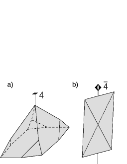
Figure 1: Crystals with (a) $C_{4}$ and (b) $S_{4}$ point groups.

Let us consider symmetry transformations in crystals with natural optical activity. According to the conditions for dual systems (see Eq. (11) in Ref. Fernandez-Corbaton and Molina-Terriza (2013)), we find that the constituent relations in Eqs. (58, 59) preserve the duality symmetry only if $\hat{\alpha}=\hat{\alpha}^{T}$. This means that the duality symmetry is broken in $C_{n}$ and $C_{nv}$ ($n\geq 3$) point groups, see Table 2.

At the same time, $\hat{\alpha}$ commutes with the helicity transformation $\hat{S}_{z}$ in $C_{n}$ and $C_{nv}$ ($n\geq 3$), while in $D_{2d}$ and $S_{4}$ commutativity between $\hat{\alpha}$ and $\hat{S}_{z}$ does not hold. The conservation of helicity in $C_{n}$ and $C_{nv}$ is supported by the scattering theorem, which states that electromagnetic forward scattering in linear systems with the discrete rotational symmetry ($n\geq 3$) can be only helicity preserving when light spreads along the principal axis Fernandez-Corbaton (2013).

The examples above demonstrate that in crystals with natural optical activity it is possible that either duality or helicity operator is the symmetry transformation but not both of them at the same time. We consider these two cases in more detail in the following sections.

IV.2.1 Conservation of helicity with broken duality

Let us consider nongeometric symmetry transformations in $C_{n}$ point groups ($n\geq 3$). The gyration tensor $\hat{\alpha}$ is given in Table 2. For illustration, a chiral crystal belonging to the $C_{4}$ point group is shown in Fig. 1 (a).

The diagonal form of $\mathcal{H}^{(\mathcal{A})}$ in Eq. (28) is brought forth by the unitary transformation

$$\psi(t,\bm{p})=\mathcal{U}_{C}\bar{\psi}(t,\bm{p})$$ (60)

(see Appendix B for explicit form of $\mathcal{U}_{C}$) that brings about

$$\bar{\mathcal{H}}^{\mathcal{A}}=\mathop{\mathrm{diag}}\nolimits\left(p_{+},-p_{-},0,-p_{+},p_{-},0\right),$$ (61)

with $p_{\pm}=p[(1\mp\alpha_{0}p)^{2}+\alpha_{2}^{2}p^{2}]^{-1/2}$.

The form of Eq. (61) suggests that in $C_{n}$ point groups the invariance algebra for the light spread along the high symmetry direction is four-dimensional $A_{4}$. In the transformed frame, the basis elements are given in Eqs. (31)–(34). However, in achiral point groups $C_{nv}$, we have additional constraint $\alpha_{0}=0$ (see Table 2), which restores the symmetry between left and right polarized states, $p_{+}=p_{-}$, and the resulting invariance algebra becomes eight-dimensional, in agreement with Eq. (77).

In order to define optical chirality, we construct the following operator in the transformed frame

$$\bar{\mathcal{Q}}_{\chi}(\bm{p})=\frac{p}{2p_{-}}\left(\bar{\mathcal{Q}}_{a}+\bar{\mathcal{Q}}_{d}\right)+\frac{p}{2p_{+}}\left(\bar{\mathcal{Q}}_{a}-\bar{\mathcal{Q}}_{d}\right),$$ (62)

which in the original basis is written as

$$\mathcal{Q}_{\chi}(\bm{p})=\begin{pmatrix}0&-i\hat{I}-i\hat{\alpha}(\hat{\bm{S}}\cdot\bm{p})\\ i\hat{I}+i\hat{\alpha}^{T}(\hat{\bm{S}}\cdot\bm{p})\end{pmatrix}.$$ (63)

We can use this operator to define optical chirality. Using $\mathcal{Q}_{A}=i\mathcal{Q}_{\chi}\partial_{t}$ in Eq. (38), optical chirality in point groups $C_{n}$, $C_{nv}$ is obtained as

$$C_{\chi}^{(c)}=\frac{1}{2}\int d^{3}p\left(\bm{D}^{*}\cdot\partial_{t}\bm{B}-\bm{B}^{*}\cdot\partial_{t}\bm{D}\right)\\ +\frac{i}{2}\int d^{3}p\left(\bm{D}^{*}\cdot\hat{\alpha}\bm{p}\times\partial_{t}\bm{B}-\bm{B}^{*}\cdot\hat{\alpha}^{T}\bm{p}\times\partial_{t}\bm{D}\right).$$ (64)

By using the constituent relations in Eqs. (58, 59), this equation can be rewritten in a compact form

$$C_{\chi}^{(c)}=-\frac{i}{2}\int d^{3}p\left(\bm{D}^{*}\cdot\varepsilon_{s}^{-1}\bm{p}\times\bm{D}+\bm{B}^{*}\cdot\mu_{s}^{-1}\bm{p}\times\bm{B}\right),$$ (65)

which is nothing but the conservation law for the helicity operator $(\bm{\mathcal{S}}\cdot\tilde{\bm{p}})$, see Eq. (99) in Appendix B.

IV.2.2 Duality symmetry without helicity transformation

The gyration tensor in point groups $S_{4}$ and $D_{2d}$ is given in Table 2. We take $\hat{\alpha}$ in the form that corresponds to $S_{4}$ group. The case of $D_{2d}$ group is obtained by setting $\alpha_{0}=0$. An example of achiral crystal with $S_{4}$ point group is demonstrated in Fig. 1 (b).

The unitary transformation that diagonalizes $\mathcal{H}^{(\mathcal{A})}$ in $S_{4}$ and $D_{2d}$ is defined as

$$\psi(t,\bm{p})=\mathcal{U}_{S}\bar{\psi}(t,\bm{p}),$$ (66)

where $\mathcal{U}_{S}$ is specified in Appendix C, which leads to the following dialgonal form in Eq. (29)

$$\bar{\mathcal{H}}^{(\mathcal{A})}=\mathop{\mathrm{diag}}\nolimits\left(-p_{1},p_{1},0,p_{1},-p_{1},0\right),$$ (67)

where $p_{1}=p[1+(\alpha_{0}^{2}+\alpha_{2}^{2})p^{2}]^{-1/2}$.

Equation (67) shows that unlike $C_{n}$ point groups, the symmetry properties of $\mathcal{H}^{\mathcal{A}}$ in $S_{4}$ and $D_{2d}$, for $\bm{p}$ along the principal axis, are similar to the case of $C_{nv}$ point groups. The invariance algebra of the symmetry transformations in $S_{4}$ and $D_{2d}$ is eight-dimensional, since the symmetry between left and right polarized states remains unbroken, which is related to the absence of optical rotation along the symmetry direction in achiral crystals Claborn et al. (2008).

Since in $S_{4}$ and $D_{2d}$ we have $\hat{\alpha}=\hat{\alpha}^{T}$ for $\bm{p}\parallel\hat{z}$, the constituent relations preserve the duality symmetry, which means that $\mathcal{Q}_{\mathrm{dual}}$ enters to the invariance algebra. This means that optical chirality in $S_{4}$ and $D_{2d}$ groups is given by Eq. (39).

We emphasize that the helicity operator $(\bm{\mathcal{S}}\cdot\tilde{\bm{p}})$ does not belong to the symmetry transformations in $S_{4}$ and $D_{2d}$ point groups even for $\bm{p}\parallel\hat{z}$. . Instead, the role of the helicity operator is played by $\mathcal{Q}_{\mathrm{h}}=-p^{-1}\mathcal{Q}_{\mathrm{dual}}\partial_{t}$, whose explicit form is given by

$$\mathcal{Q}_{\mathrm{h}}=\begin{pmatrix}(\bm{\mathcal{S}}\cdot\tilde{\bm{p}})\hat{\varepsilon}^{-1}(\bm{p})&0\\ 0&(\bm{\mathcal{S}}\cdot\tilde{\bm{p}})\hat{\mu}^{-1}(\bm{p})\end{pmatrix},$$ (68)

where we used the identity $i\partial_{t}\equiv\mathcal{H}^{(\mathcal{A})}$ together with Eq. (28).

Table 2: Gyration tensor in different point groups

Gyration tensor $\hat{\alpha}$	Point groups	Gyration tensor $\hat{\alpha}$	Point groups
$\left(\begin{array}[]{ccc}\alpha_{0}&\alpha_{2}&0\\ \alpha_{2}&-\alpha_{0}&0\\ 0&0&0\end{array}\right)$	Tetragonal: $S_{4}$ ($\bar{4}$)	$\left(\begin{array}[]{ccc}0&\alpha_{2}&0\\ \alpha_{2}&0&0\\ 0&0&0\end{array}\right)$	Tetragonal: $D_{2d}$ ($\bar{4}2m$)
$\left(\begin{array}[]{ccc}\alpha_{0}&\alpha_{2}&0\\ -\alpha_{2}&\alpha_{0}&0\\ 0&0&\alpha_{1}\end{array}\right)$	Tetragonal: $C_{4}$ ($4$)	$\left(\begin{array}[]{ccc}0&\alpha_{2}&0\\ -\alpha_{2}&0&0\\ 0&0&0\end{array}\right)$	Tetragonal: $C_{4v}$ ($4mm$)
	Trigonal: $C_{3}$ ($3$)		Trigonal: $C_{3v}$ ($3m$)
	Hexagonal: $C_{6}$ ($6$)		Hexagonal: $C_{6v}$ ($6mm$)
$\left(\begin{array}[]{ccc}\alpha_{0}&0&0\\ 0&\alpha_{0}&0\\ 0&0&\alpha_{1}\end{array}\right)$	Tetragonal: $D_{4}$ ($422$)	$\left(\begin{array}[]{ccc}\alpha_{0}&0&0\\ 0&\alpha_{0}&0\\ 0&0&\alpha_{0}\end{array}\right)$
	Trigonal: $D_{3}$ ($32$)		Cubic: $T$ ($23$), $O$ ($432$)
	Hexagonal: $D_{6}$ ($622$)

IV.3 Lack of duality symmetry and helicity

In systems with low crystalline symmetry, the definition of optical chirality meets with difficulties. For illustration, we consider a simple example of the non-gyrotropic system that belongs to the orthorhombic crystal class. In this case, the electric permittivity and magnetic permeability tensors in principal axes are given by diagonal matrices $\hat{\varepsilon}=\mathop{\mathrm{diag}}\nolimits(\varepsilon_{1},\varepsilon_{2},\varepsilon_{3})$ and $\hat{\mu}=\mathop{\mathrm{diag}}\nolimits(\mu_{1},\mu_{2},\mu_{3})$.

For the diagonal $\hat{\varepsilon}$ and $\hat{\mu}$, the symmetry analysis developed in Sec. III remains valid along the principal axes. We consider one particular direction taken as $\hat{z}$-axis, and fix $\bm{p}=p\hat{z}$. To implement the general formalism in Eqs. (26)–(28), we use the nonunitary transformation $\psi=\mathcal{N}_{2}\bar{\psi}$ ($\mathcal{N}_{2}$ is specified in Appendix D), which leads to the diagonal form

$$\bar{\mathcal{H}}^{(\mathcal{A})}=\left(\frac{-p}{\sqrt{\varepsilon_{1}\mu_{2}}},\frac{p}{\sqrt{\varepsilon_{2}\mu_{1}}},0\frac{p}{\sqrt{\varepsilon_{1}\mu_{2}}},\frac{-p}{\sqrt{\varepsilon_{2}\mu_{1}}},0\right),$$ (69)

prescribed by Eq. (29). In accordance with Eq. (77), the symmetry transformations in the transformed frame are given in Eqs. (31)–(34).

However, neither duality nor helicity operators can be expressed in this basis. To illustrate this fact, we apply the inverse transformation to the initial basis, $\bar{\psi}=\mathcal{N}_{2}^{-1}\psi$, to the operators in Eqs. (31)–(34). Straightforward calculation yields the following basis operators in the initial frame

$$\mathcal{Q}_{3}^{\prime}=\rho\mathcal{N}\bar{\mathcal{Q}}_{a}\,\mathcal{N}_{2}^{-1}, \qquad\mathcal{Q}_{6}^{\prime}=\rho\mathcal{N}\bar{\mathcal{Q}}_{b}\,\mathcal{N}_{2}^{-1},$$ (70)

$$\mathcal{Q}_{7}^{\prime}=\rho\mathcal{N}\bar{\mathcal{Q}}_{c}\,\mathcal{N}_{2}^{-1}, \qquad\mathcal{Q}_{8}^{\prime}=\rho\mathcal{N}\bar{\mathcal{Q}}_{d}\,\mathcal{N}_{2}^{-1},$$ (71)

where the explicit form of these matrices is given in Appendix D. Now if we take the limiting case of isotropic system, $\varepsilon_{i}=\mu_{i}=1$ ($i=1,2$), we will find that Eqs. (70, 71) are mapped to the commutative subalgebra $\left\{\mathcal{Q}_{3},\mathcal{Q}_{6},\mathcal{Q}_{7},\mathcal{Q}_{8}\right\}$ of $A_{8}$, see Eqs. (12)–(15), which contains neither $\mathcal{Q}_{2}$ (duality) nor $\mathcal{Q}_{5}$ (helicity) operators.

From Eqs. (70, 71), we find that the only possible $T$-even and $P$-odd combinations are $p_{z}\mathcal{Q}_{6}^{\prime}$ and $p_{z}\mathcal{Q}_{7}^{\prime}$. However, substitution of these expressions into Eq. (38) gives zero. Therefore, we make a conclusion that it is not possible to construct optical chirality in the system, where the both duality and helicity are absent. This result is supported by the conclusions in Ref. Fernandez-Corbaton (2013) that helicity-conserving scattering theorems do not exist for systems with one and two fold principal rotational axes.

V Summary

We examined symmetry properties of the Maxwell’s equations in various types of gyrotropic media making a particular accent on the conservation of optical chirality. For this purpose, we extended the formalism of nongeometric symmetries in vacuum to medium with given constituent relations. Within this approach, a conclusion about the conservation of optical chirality is reduced to the analysis of the invariance algebra of the nongeometric symmetries and establishing possible isomorphism between some elements of this algebra and operators of the helicity and duality symmetries in vacuum. The advantage of this approach is that it suggests a straightforward way to derive various conservation laws related to the invariance algebra of the Maxwell’s equations.

Using this method, we constructed the conservation law for optical chirality in isotropic chiral media, as well as in trigonal, tetragonal, and hexagonal crystals along the symmetry direction. In particular, we demonstrated that in the gyrotropic crystals with natural optical activity, which belong to the point groups $C_{n}$ or $C_{nv}$, only the optical helicity retains along the principal axis, whereas in the case of achiral optically active crystals of the point symmetry $S_{4}$ or $D_{2d}$ only the duality transformation remains. In all of the presented examples, except the achiral materials, we deal with a reduction of the original eight-dimensional invariance algebra in the vacuum to the four-dimensional basis set. Additionally, we give an example of the medium where none of these symmetries is conserved.

Appendix A Derivation of the invariance algebra in medium

We highlight the derivation of the invariance algebra for the Maxwell’s equations in (23, 24). Any symmetry transformation $\mathcal{Q}_{A}(\bm{p})$ that transforms a solution $\psi(t,\bm{p})=(\bm{D}(t,\bm{p}),\bm{B}(t,\bm{p}))$ of Eqs. (23, 24) into another solution $\psi^{\prime}=\mathcal{Q}_{A}\psi$ should satisfy the following invariance conditions

$$[\mathcal{L}^{(\mathcal{A})},\mathcal{Q}_{A}] = g_{11}\mathcal{L}^{(\mathcal{A})}+g_{12}\mathcal{L},$$ (72)

$$\left[\mathcal{L},\mathcal{Q}_{A}\right] = g_{21}\mathcal{L}^{(\mathcal{A})}+g_{22}\mathcal{L},$$ (73)

where $\mathcal{L}$ and $\mathcal{L}^{(\mathcal{A})}$ are determined in Eqs. (11) and (26), and $g_{ij}$ denote some arbitrary operators acting on $\psi$.

For the diagonal operators in Eqs. (29, 30), we can find the invariance algebra. Given the fact that ${\cal Q}_{A}(\bm{p})$ depends only on $\bm{p}$, the invariance conditions in the transformed frame take the following reduced form

$$[\bar{{\cal H}}^{(\mathcal{A})},\bar{\cal Q}_{A}] = \bar{g}_{12}\bar{\mathcal{L}},$$ (74)

$$\left[\bar{{\cal L}},\bar{\cal Q}_{A}\right] = \bar{g}_{22}\bar{{\cal L}},$$ (75)

where $\bar{{\cal Q}}_{A}=\mathcal{N}^{-1}{\cal Q}_{A}\mathcal{N}$, and $\bar{g}_{12}$ and $\bar{g}_{22}$ denote some redefined operators.

The most general form of $\bar{\cal Q}_{A}$ imposed by Eq. (75) is rendered as

$$\bar{\cal Q}_{A}=\left(\begin{array}[]{cccccc}q_{11}&q_{12}&0&q_{14}&q_{15}&0\\ q_{21}&q_{22}&0&q_{24}&q_{25}&0\\ 0&0&0&0&0&0\\ q_{41}&q_{42}&0&q_{44}&q_{45}&0\\ q_{51}&q_{52}&0&q_{54}&q_{55}&0\\ 0&0&0&0&0&0\end{array}\right)+\mathcal{F}\bar{\mathcal{L}},$$ (76)

with some operator $\mathcal{F}$. The last term in this equation can be safely dropped since it does not contribute into finding of the invariance algebra Fushchich and Nikitin (1987). Then, the first invariance condition given by Eq. (74) is satisfied for commutative $\bar{{\cal H}}^{(\mathcal{A})}$ and $\bar{\cal Q}_{A}$.

To identify the invariance algebra, we explicitly calculate the commutator in Eq. (74)

$$\left[\bar{{\cal H}}^{(\mathcal{A})},\bar{\cal Q}_{A}\right]=\left(\begin{array}[]{cccccc}0&q_{12}(\omega_{2}-\omega_{1})&0&q_{14}(\omega_{4}-\omega_{1})&q_{15}(\omega_{5}-\omega_{1})&0\\ q_{21}(\omega_{1}-\omega_{2})&0&0&q_{24}(\omega_{4}-\omega_{2})&q_{25}(\omega_{5}-\omega_{2})&0\\ 0&0&0&0&0&0\\ q_{41}(\omega_{1}-\omega_{4})&q_{42}(\omega_{2}-\omega_{4})&0&0&q_{45}(\omega_{5}-\omega_{4})&0\\ q_{51}(\omega_{1}-\omega_{5})&q_{52}(\omega_{2}-\omega_{5})&0&q_{54}(\omega_{4}-\omega_{5})&0&0\\ 0&0&0&0&0&0\end{array}\right),$$ (77)

where Eq. (29) is used. The number of basis elements in the invariance algebra depends on the symmetry relations between $\omega_{i}$ that occur in Eq. (29). When there are no any degeneracies between $\omega_{i}$ (the lowest symmetry case), all the matrices $\bar{\cal Q}_{A}$, which commute with $\bar{{\cal H}}^{(\mathcal{A})}$, have diagonal form with four free parameters

$$\bar{\cal Q}_{A}=\mathop{\mathrm{diag}}\nolimits(q_{11},q_{22},0,q_{44},q_{55},0),$$ (78)

which corresponds to the set of basis operators in Eq. (32–34).

Appendix B Transformations in point groups $C_{n}$, $C_{nv}$, and $D_{n}$, $n\geq 3$

In the point groups $C_{n}$, $C_{nv}$, and $D_{n}$, the inverse tensors $\hat{\varepsilon}^{-1}$ and $\hat{\mu}^{-1}$ in Eq. (28) are given by

$$\hat{\varepsilon}^{-1}=\frac{1}{\varepsilon_{\perp}d}\left(\begin{array}[]{ccc}1+i\alpha_{2}p&i\alpha_{0}p&0\\ -i\alpha_{0}p&1+i\alpha_{2}p&0\\ 0&0&0\end{array}\right)+\frac{1}{\varepsilon_{\parallel}}\left(\begin{array}[]{ccc}0&0&0\\ 0&0&0\\ 0&0&1\end{array}\right),$$ (85)

$$\hat{\mu}^{-1}=\frac{1}{\mu_{\perp}d^{*}}\left(\begin{array}[]{ccc}1-i\alpha_{2}p&i\alpha_{0}p&0\\ -i\alpha_{0}p&1-i\alpha_{2}p&0\\ 0&0&0\end{array}\right)+\frac{1}{\mu_{\parallel}}\left(\begin{array}[]{ccc}0&0&0\\ 0&0&0\\ 0&0&1\end{array}\right),$$ (92)

where $d=1-|a|^{2}+2i\alpha_{2}p$ and $a=(\alpha_{0}+i\alpha_{2})p$. In what follows, we will use the units where $\varepsilon_{\perp}=\mu_{\perp}=1$.

The matrix $\mathcal{H}^{(\mathcal{A})}$ in Eq. (28) is diagonalized in two steps. First, we make a transformation to the helicity basis

$$\mathcal{H}^{(\mathcal{A})}_{\Lambda}=\mathcal{U}^{{\dagger}}_{\Lambda}\mathcal{H}^{(\mathcal{A})}\mathcal{U}_{\Lambda},$$ (93)

where $\mathcal{U}_{\Lambda}=\sigma_{0}\otimes\hat{U}_{\Lambda}$, see Eq. (35), which gives

$$\mathcal{H}^{(\mathcal{A})}_{\Lambda}=\begin{pmatrix}0&i\hat{M}^{*}\\ -i\hat{M}&0\end{pmatrix},$$ (94)

where $\hat{M}=\mathop{\mathrm{diag}}\nolimits\left(-p/(1+a^{*}),p/(1+a),0\right)$. Second, we apply a unitary transformation

$$\bar{\mathcal{H}}^{(\mathcal{A})}=\mathcal{U}_{M}^{{\dagger}}\mathcal{H}^{(\mathcal{A})}_{\Lambda}\mathcal{U}_{M},$$ (95)

with

$$\mathcal{U}_{M}=\frac{1}{\sqrt{2}}\left(\begin{array}[]{cccccc}-\dfrac{ip}{p_{+}(1-a)}&0&0&\dfrac{ip}{p_{+}(1-a)}&0&0\\ 0&-\dfrac{ip}{p_{-}(1+a^{*})}&0&0&\dfrac{ip}{p_{-}(1+a^{*})}&0\\ 0&0&\sqrt{2}&0&0&0\\ 1&0&0&1&0&0\\ 0&1&0&0&1&0\\ 0&0&0&0&0&\sqrt{2}\end{array}\right),$$ (96)

which gives the diagonal form Eq. (61). Altogether, the whole transformation in Eq. (60) is rendered by

$$\mathcal{U}_{C}=\mathcal{U}_{\Lambda}\mathcal{U}_{M}.$$ (97)

Let us note that the conservation law for the optical chirality in Eq. (65) is obtained directly, if we notice that the inverse transformation of $\bar{\mathcal{Q}}_{b}$ in Eq. (32) gives the helicity operator

$$(\bm{\mathcal{S}}\cdot\tilde{\bm{p}})=\mathcal{U}_{C}\,\bar{\mathcal{Q}}_{b}\,\mathcal{U}_{C}^{{\dagger}},$$ (98)

then optical chirality can be defined similar to Eq. (20)

$$C_{\chi}^{(c)}=\frac{1}{2}\int d^{3}p\,\psi^{{\dagger}}(t,\bm{p})\,(\bm{\mathcal{S}}\cdot\bm{p})\,\psi(t,\bm{p}),$$ (99)

which corresponds to Eq. (65).

Appendix C Transformations in point groups $S_{4}$ and $D_{2d}$

In achiral point groups $S_{4}$ and $D_{2d}$, we have the following $\hat{\varepsilon}^{-1}$ and $\hat{\mu}^{-1}$ in Eq. (28)

$$\hat{\varepsilon}^{-1}=\frac{1}{\varepsilon_{\perp}(1+|a|^{2})}\left(\begin{array}[]{ccc}1-i\alpha_{2}p&i\alpha_{0}p&0\\ i\alpha_{0}p&1+i\alpha_{2}p&0\\ 0&0&0\end{array}\right)+\frac{1}{\varepsilon_{\parallel}}\left(\begin{array}[]{ccc}0&0&0\\ 0&0&0\\ 0&0&1\end{array}\right),$$ (106)

$$\hat{\mu}^{-1}=\frac{1}{\mu_{\perp}(1+|a|^{2})}\left(\begin{array}[]{ccc}1-i\alpha_{2}p&i\alpha_{0}p&0\\ i\alpha_{0}p&1+i\alpha_{2}p&0\\ 0&0&0\end{array}\right)+\frac{1}{\mu_{\parallel}}\left(\begin{array}[]{ccc}0&0&0\\ 0&0&0\\ 0&0&1\end{array}\right).$$ (113)

In order to diagonalize $\mathcal{H}^{(\mathcal{A})}$ in Eq. (28), we apply a sequence of unitary transformations

$$\mathcal{U}_{S}=\mathcal{U}_{\Lambda}\mathcal{U}_{N}\mathcal{U}_{2},$$ (114)

where $\mathcal{U}_{\Lambda}=\sigma_{0}\otimes\hat{U}_{\Lambda}$, $\mathcal{U}_{N}=\sigma_{0}\otimes\hat{U}_{N}$, and $\mathcal{U}_{2}=\hat{U}_{2}\otimes{I}$ with

$$\hat{U}_{\Lambda}=\left(\begin{array}[]{ccc}-\dfrac{1}{\sqrt{2}}&\dfrac{1}{\sqrt{2}}&0\\ \dfrac{i}{\sqrt{2}}&\dfrac{i}{\sqrt{2}}&0\\ 0&0&1\end{array}\right),\qquad\hat{U}_{N}=\left(\begin{array}[]{ccc}\dfrac{|a|}{\sqrt{2}a^{*}}\dfrac{1-\sqrt{1+|a|^{2}}}{\sqrt{1+|a|^{2}-\sqrt{1+|a|^{2}}}}&\dfrac{|a|}{\sqrt{2}a^{*}}\dfrac{1+\sqrt{1+|a|^{2}}}{\sqrt{1+|a|^{2}+\sqrt{1+|a|^{2}}}}&0\\ \dfrac{|a|}{\sqrt{2}}\dfrac{1}{\sqrt{1+|a|^{2}-\sqrt{1+|a|^{2}}}}&\dfrac{|a|}{\sqrt{2}}\dfrac{1}{\sqrt{1+|a|^{2}+\sqrt{1+|a|^{2}}}}&0\\ 0&0&1\end{array}\right).$$ (115)

Note that $\mathcal{U}_{N}$ commutes with $\bar{\mathcal{L}}=\mathcal{U}^{{\dagger}}_{\Lambda}\,\mathcal{L}\,\mathcal{U}_{\Lambda}$.

Appendix D Orthorhombic crystal

The diagonalization in Eq. (29) is carried out by applying

$$\mathcal{N}=\begin{pmatrix}-\sqrt{\frac{\varepsilon_{1}}{\varepsilon_{1}+\mu_{2}}}&0&0&\sqrt{\frac{\varepsilon_{1}}{\varepsilon_{1}+\mu_{2}}}&0&0\\ 0&-\sqrt{\frac{\varepsilon_{2}}{\varepsilon_{2}+\mu_{1}}}&0&0&\sqrt{\frac{\varepsilon_{2}}{\varepsilon_{2}+\mu_{1}}}&0\\ 0&0&1&0&0&0\\ 0&\sqrt{\frac{\mu_{1}}{\mu_{1}+\varepsilon_{2}}}&0&0&\sqrt{\frac{\mu_{1}}{\mu_{1}+\varepsilon_{2}}}&0\\ \sqrt{\frac{\mu_{2}}{\mu_{2}+\varepsilon_{1}}}&0&0&\sqrt{\frac{\mu_{2}}{\mu_{2}+\varepsilon_{1}}}&0&0\\ 0&0&0&0&0&1\end{pmatrix}$$ (116)

that commutes with $\mathcal{L}$ in Eq. (11).

The explicit form of $\mathcal{Q}_{A}^{\prime}$ in Eqs. (70, 71) is given by the following expressions

$$\mathcal{Q}_{3}^{\prime}=\left(\begin{array}[]{cccccc}0&0&0&0&-\frac{\varepsilon_{1}+\mu_{2}}{2\sqrt{\varepsilon_{1}\mu_{2}}}&0\\ 0&0&0&-\frac{\varepsilon_{2}+\mu_{1}}{2\sqrt{\varepsilon_{2}\mu_{1}}}&0&0\\ 0&0&0&0&0&0\\ 0&-\frac{\varepsilon_{2}+\mu_{1}}{2\sqrt{\varepsilon_{2}\mu_{1}}}&0&0&0&0\\ -\frac{\varepsilon_{1}+\mu_{2}}{2\sqrt{\varepsilon_{1}\mu_{2}}}&0&0&0&0&0\\ 0&0&0&0&0&0\end{array}\right), \quad\mathcal{Q}_{8}^{\prime}=\left(\begin{array}[]{cccccc}0&0&0&0&\frac{\varepsilon_{1}+\mu_{2}}{2\sqrt{\varepsilon_{1}\mu_{2}}}&0\\ 0&0&0&-\frac{\varepsilon_{2}+\mu_{1}}{2\sqrt{\varepsilon_{2}\mu_{1}}}&0&0\\ 0&0&0&0&0&0\\ 0&-\frac{\varepsilon_{2}+\mu_{1}}{2\sqrt{\varepsilon_{2}\mu_{1}}}&0&0&0&0\\ \frac{\varepsilon_{1}+\mu_{2}}{2\sqrt{\varepsilon_{1}\mu_{2}}}&0&0&0&0&0\\ 0&0&0&0&0&0\end{array}\right),$$ (129)

$$\mathcal{Q}_{6}^{\prime}=\mathop{\mathrm{diag}}\nolimits\left(-\frac{\varepsilon_{1}+\mu_{2}}{2\varepsilon_{1}},\frac{\varepsilon_{2}+\mu_{1}}{2\varepsilon_{2}},0,\frac{\varepsilon_{2}+\mu_{1}}{2\mu_{1}},-\frac{\varepsilon_{1}+\mu_{2}}{2\mu_{2}},0\right), \quad\mathcal{Q}_{7}^{\prime}=\left(\frac{\varepsilon_{1}+\mu_{2}}{2\varepsilon_{1}},\frac{\varepsilon_{2}+\mu_{1}}{2\varepsilon_{2}},0,\frac{\varepsilon_{2}+\mu_{1}}{2\mu_{1}},\frac{\varepsilon_{1}+\mu_{2}}{2\mu_{2}},0\right).$$ (130)

References

- Kelvin (1904) L. Kelvin, Baltimore Lectures on Molecular Dynamics and the Wave Theory of Light (CJ Clay & Sons, London, 1904).
- Dreiling and Gay (2014) J. M. Dreiling and T. J. Gay, Phys. Rev. Lett. 113, 118103 (2014).
- Lipkin (1964) D. M. Lipkin, J. Math. Phys. 5, 696 (1964).
- Morgan (1964) T. A. Morgan, J. Math. Phys. 5, 1659 (1964).
- Kibble (1965) T. W. B. Kibble, J. Math. Phys. 6, 1022 (1965).
- Barron (1986) L. Barron, Chem. Phys. Lett. 123, 423 (1986).
- Barron (2004) L. D. Barron, Molecular light scattering and optical activity (Cambridge University Press, 2004).
- Fushchich and Nikitin (1987) W. I. Fushchich and A. G. Nikitin, Symmetries of Maxwell’s Equations, Mathematics and its Applications (Springer Netherlands, 1987).
- Krivskii and Simulik (1989a) I. Y. Krivskii and V. M. Simulik, Theor. Math. Phys. 80, 864 (1989a).
- Krivskii and Simulik (1989b) I. Y. Krivskii and V. M. Simulik, Theor. Math. Phys. 80, 912 (1989b).
- Ibragimov (2008) N. H. Ibragimov, Acta Appl. Math. 105, 157 (2008).
- Cameron and Barnett (2012) R. P. Cameron and S. M. Barnett, New J. Phys. 14, 123019 (2012).
- Bliokh et al. (2013) K. Y. Bliokh, A. Y. Bekshaev, and F. Nori, New J. Phys. 15, 033026 (2013).
- Cameron (2014) R. P. Cameron, On the angular momentum of light, Ph.D. thesis, School of Physics and Astronomy, College of Science of Engineering, University of Glasgow (2014).
- Barnett (2014) S. M. Barnett, New J. Phys. 16, 093008 (2014).
- Philbin (2013) T. G. Philbin, Phys. Rev. A 87, 043843 (2013).
- Calkin (1965) M. G. Calkin, American Journal of Physics 33, 958 (1965).
- Zwanziger (1968) D. Zwanziger, Phys. Rev. 176, 1489 (1968).
- Drummond (1999) P. D. Drummond, Physical Review A 60, R3331 (1999).
- Drummond (2006) P. D. Drummond, Journal of Physics B: Atomic, Molecular and Optical Physics 39, S573 (2006).
- Tang and Cohen (2010) Y. Tang and A. E. Cohen, Phys. Rev. Lett. 104, 163901 (2010).
- Hendry et al. (2010) E. Hendry, T. Carpy, J. Johnston, M. Popland, R. Mikhaylovskiy, A. Lapthorn, S. Kelly, L. Barron, N. Gadegaard, and M. Kadodwala, Nature Nanotech. 5, 783 (2010).
- Tang and Cohen (2011) Y. Tang and A. E. Cohen, Science 332, 333 (2011).
- Hendry et al. (2012) E. Hendry, R. V. Mikhaylovskiy, L. D. Barron, M. Kadodwala, and T. J. Davis, Nano Lett. 12, 3640 (2012).
- Kamenetskii et al. (2013) E. O. Kamenetskii, R. Joffe, and R. Shavit, Phys. Rev. E 87, 023201 (2013).
- Tomita et al. (2014) S. Tomita, K. Sawada, A. Porokhnyuk, and T. Ueda, Phys. Rev. Lett. 113, 235501 (2014).
- Yao and Padgett (2011) A. Yao and M. Padgett, Advances in Optics and Photonics 3, 161 (2011).
- Bliokh and Nori (2015) K. Y. Bliokh and F. Nori, Phys. Rep. 592, 1 (2015).
- Afanasiev and Stepanovsky (1996) G. N. Afanasiev and Y. P. Stepanovsky, Nuovo Cimento A 109, 271 (1996).
- Bliokh and Nori (2011) K. Y. Bliokh and F. Nori, Phys. Rev. A 83, 021803 (2011).
- Coles and Andrews (2012) M. M. Coles and D. L. Andrews, Phys. Rev. A 85, 063810 (2012).
- Cameron et al. (2012) R. P. Cameron, S. M. Barnett, and A. M. Yao, New J. of Phys. 14, 053050 (2012).
- Barnett et al. (2012) S. M. Barnett, R. P. Cameron, and A. M. Yao, Phys. Rev. A 86, 013845 (2012).
- Bliokh et al. (2014a) K. Y. Bliokh, Y. S. Kivshar, and F. Nori, Phys. Rev. Lett. 113, 033601 (2014a).
- Bliokh et al. (2014b) K. Y. Bliokh, J. Dressel, and F. Nori, New Journal of Physics 16, 093037 (2014b).
- Bliokh et al. (2015) K. Y. Bliokh, F. Rodríguez-Fortuño, F. Nori, and A. V. Zayats, Nature Photonics 9, 796 (2015).
- Bliokh et al. (2016) K. Y. Bliokh, A. Y. Bekshaev, and F. Nori, New Journal of Physics 18, 089503 (2016).
- Dressel et al. (2015) J. Dressel, K. Y. Bliokh, and F. Nori, Physics Reports 589, 1 (2015).
- Ragusa (1994) S. Ragusa, J. Phys. A: Math. Gen. 27, 2887 (1994).
- Ragusa (1996) S. Ragusa, Brazilian Journal of Physics 26, 411 (1996).
- Fernandez-Corbaton and Molina-Terriza (2013) I. Fernandez-Corbaton and G. Molina-Terriza, Phys. Rev. B 88, 085111 (2013).
- Fernandez-Corbaton (2013) I. Fernandez-Corbaton, Optics express 21, 29885 (2013).
- Robinson (2012) D. Robinson, A Course in the Theory of Groups, Vol. 80 (Springer Science & Business Media, 2012).
- Berry (2009) M. V. Berry, J. Opt A: Pure Appl. Opt. 11, 094001 (2009).
- Claborn et al. (2008) K. Claborn, C. Isborn, W. Kaminsky, and B. Kahr, Angewandte Chemie International Edition 47, 5706 (2008).
- Condon (1937) E. U. Condon, Rev. Mod. Phys. 9, 432 (1937).
- Born (1972) M. Born, Optik Springer-Verlag (Berlin, 1972).
- Fedorov (1959) F. Fedorov, Opt. Spectrosc. 6, 49 (1959).
- Fedorov (1976) F. I. Fedorov, Teorija girotropii (Izd. Nauka i Technika, 1976).
- Post (1962) E. J. Post, Formal structure of electromagnetics: general covariance and electromagnetics (North-Holland Publishing Company, Amsterdam, 1962).
- Rado and Folen (1962) G. T. Rado and V. J. Folen, J. Appl. Phys. 33, 1126 (1962).
- Jaggard et al. (1979) D. Jaggard, A. Mickelson, and C. Papas, Appl. Phys. 18, 211 (1979).
- Hornreich and Shtrikman (1968) R. M. Hornreich and S. Shtrikman, Phys. Rev. 171, 1065 (1968).
- Hornreich (1968) R. M. Hornreich, J. Appl. Phys. 39, 432 (1968).
- Lekner (1996) J. Lekner, Pure and Applied Optics: Journal of the European Optical Society Part A 5, 417 (1996).
- Fisanov (2007) V. V. Fisanov, Journal of Communications Technology and Electronics 52, 1006 (2007).
- Cho (2015) K. Cho, ArXiv e-prints (2015), arXiv:1501.01078 .
- Bialynicki-Birula (1996) I. Bialynicki-Birula, in Coherence and Quantum Optics VII (Springer, 1996) pp. 313–322.
- Note (1) If the relation holds in medium with constituent relations in Eqs. (40–43), this medium is self-dual according to Ref. Fernandez-Corbaton and Molina-Terriza (2013). In this case, we can also rewrite Eq. (53) in the form of conservation law for redefined and .
- Hu et al. (1987) C.-R. Hu, G. W. Kattawar, M. E. Parkin, and P. Herb, Applied optics 26, 4159 (1987).
- Glazer and Burns (2013) M. Glazer and G. Burns, Space Groups for Solid State Scientists (Elsevier Science, 2013).
- Note (2) Here, under the helicity we mean the projection of the spin onto the direction of propagation, . We note that to discuss the physical helicity expressed through the difference in population of left and right polarized photons, one has to construct a photon wave function in chiral crystals with and groups, which is, however, beyond the scope of our symmetry analysis.