Almost all non-archimedean Kakeya sets have measure zero

Abstract

We study Kakeya sets over local non-archimedean fields with a probabilistic point of view: we define a probability measure on the set of Kakeya sets as above and prove that, according to this measure, almost all non-archimedean Kakeya sets are neglectable according to the Haar measure. We also discuss possible relations with the non-archimedean Kakeya conjecture.

At the beginning of the 20th century, Kakeya asks how small can be a subset of $\mathbb{R}^{2}$ obtained by rotating a needle of length $1$ continuously through $360$ degrees within it and returning to its original position. A set satisfying the above requirement is today known as a Kakeya set (or sometimes Kakeya needle set) in $\mathbb{R}^{2}$. In 1928, Besikovitch [2] constructed a subset of $\mathbb{R}^{2}$ with Lebesgue measure zero containing a unit length segment in each direction and derived from this the existence of Kakeya sets with arbitrary small positive Lebesgue measure. Since this, Kakeya sets have received much attention because they have connections with important questions in harmonic analysis. In particular, lower bounds on the size of a Kakeya set have been found: it has been notably established that any Kakeya set in $\mathbb{R}^{2}$ must have Hausdorff dimension $2$ (see [7, Theorem 2] for a short and elegant proof).

Kakeya’s problem extends readily to higher dimensions: a Besikovitch set in $\mathbb{R}^{d}$ is a subset of $\mathbb{R}^{d}$ containing a unit length segment in each direction while a Kakeya set in $\mathbb{R}^{d}$ is a set obtained by rotating continuously a needle of length $1$ is all directions (parametrized either by the $(d{-}1)$-dimensional sphere of the $(d{-}1)$-dimensional projective space). We refer to §1.1.1 for precise definitions. Kakeya sets in $\mathbb{R}^{d}$ with Lebesgue measure zero exist as well: the product of $\mathbb{R}^{d-2}$ by a neglectable Kakeya set in $\mathbb{R}^{2}$ makes the job. As for lower bounds, it has been proved by Wolff [9] that a Kakeya set in $\mathbb{R}^{d}$ has Hausdorff dimension $\geqslant\frac{d+2}{2}$. More recently Katz and Tao [8] improved the lower bound to $(2-\sqrt{2})(d-4)+3$. Experts however believe that these results are far from being optimal and actually conjecture that a Kakeya set in $\mathbb{R}^{d}$ should always have Hausdorff dimension $d$: this is the so-called Kakeya conjecture.

More recently Kakeya’s problem was extended over other fields. The first case of interest was that of finite fields and was first considered in [9] by Wolff. Given a finite field $\mathbb{F}_{q}$, a Besikovitch set in $\mathbb{F}_{q}^{d}$ is a subset of $\mathbb{F}_{q}^{d}$ containing an affine line in each direction (note that the length condition has gone). Wolff wondered whether there exists a positive constant $c_{d}$ depending only $d$ such that any Besikovitch set in $\mathbb{F}_{q}^{d}$ contains at least $c_{d}\cdot q^{d}$ elements. A positive answer (leading to $c_{d}=\frac{1}{d!}$) was given by Dvir in his famous paper [4].

In [5], Ellenberg, Oberlin and Tao introduced Besikovitch sets over $\mathbb{F}_{q}[[t]]$ and asked whether there exists such a set whose Haar measure is zero. Dummit and Hablicsek addressed this question in [3] and gave to it a positive answer: they proved that, for all $d\geqslant 2$ and all finite field $\mathbb{F}_{q}$, there does exist a zero-measure Besikovitch set in $\mathbb{F}_{q}[[t]]^{d}$. They more generally defined Besikovitch sets over any ring $R$ admitting a Haar measure $\mu$ for which $\mu(R)$ is finite and, for those rings, they stated a straightforward analogue of the Kakeya conjecture. Apart from $\mathbb{F}_{q}[[t]]$, an interesting ring $R$ which falls within Dummit and Hablicsek’s framework is $R=\mathbb{Z}_{p}$, the ring of $p$-adic integers. Dummit and Hablicsek then proved the Kakeya conjecture in dimension $2$ for $R=\mathbb{F}_{q}[[t]]$ and $R=\mathbb{Z}_{p}$. The existence of zero-measure Besikovitch sets over $\mathbb{Z}_{p}$ was proved more recently by Fraser in [6].

The general aim of this paper is to study further the size of Kakeya/Besikovitch sets over non-archimedean local fields, i.e. $\mathbb{F}_{q}((t))=\text{\rm Frac}\>\mathbb{F}_{q}[[t]]$, $\mathbb{Q}_{p}=\text{\rm Frac}\>\mathbb{Z}_{p}$ and their extensions. Our main originality is that we adopt a probabilistic point of view.

Let us describe more precisely our results. Let $K$ be a fixed non-archimedean local field: similarly to $\mathbb{R}$, it is equipped with an absolute value which turns it into a topological locally compact field. It is thus equipped with a Haar measure $\mu$ giving a finite mass to any bounded subset. Since $K$ is non-archimedean, the unit ball $R$ of $K$ is a subring of $K$ (it is $\mathbb{F}_{q}[[t]]$ when $K=\mathbb{F}_{q}((t))$ and $\mathbb{Z}_{p}$ when $K=\mathbb{Q}_{p}$); we normalize $\mu$ so that $\mu(R)=1$. In this setting, we provide a definition for Kakeya sets and Besikovitch sets and endow the set of Kakeya sets included in $R^{d}$ with a probability measure, giving this way a precise sense to the notion of random non-archimedean Kakeya set. Our main theorem is the following.

Theorem 1 (cf Corollary 1.19).

Almost all Kakeya sets sitting in $R^{d}$ have measure zero.

We emphasize that the above theorem concerns actual Kakeya sets (and not Besikovitch sets). It then shows a clear dichotomy between the archimedean and the non-archimedean setup: in the former, Kakeya sets have necessarily positive measure (through it can be arbitrarily small) while, in the latter, almost all of them have measure zero.

We will deduce Theorem 1 from a much more accurate result providing an exact value for the average size of $\varepsilon$-neighbourhoods of Kakeya sets. Before stating (a weak version of) it, recall that the $\varepsilon$-neighbourhood of a subset $N\subset K^{d}$ consists of points whose distance to $N$ is at most $\varepsilon$. Let $q$ be the cardinality of the residue field of $K$, i.e. of $q=\text{\rm Card}\>R/\mathfrak{m}$ where $\mathfrak{m}$ is the open unit ball in $K$. When $R=\mathbb{F}_{q}((t))$, we can check that $\mathfrak{m}=t\cdot\mathbb{F}_{q}[[t]]$, so that $q$ is indeed $q$. Similarly when $R=\mathbb{Q}_{p}$, we have $\mathfrak{m}=p\mathbb{Z}_{p}$ and $q$ is equal to $p$.

Theorem 2 (cf Proposition 1.23).

The expected value of the Haar measure of the $\varepsilon$-neighbourhood of a random Kakeya set sitting in $R^{d}$ is equivalent to:

$$\frac{2\cdot(q^{d}-1)}{(q-1)(q^{d-1}-1)}\cdot\frac{1}{|\log_{q}\varepsilon|}$$

when $\varepsilon$ goes to $0$.

This refined version of Theorem 1 seems to us quite interesting because it underlines that, although Kakeya sets tend to be neglectable according to the Haar measure, they are not that small on average as reflected by the logarithmic decay with respect to $\varepsilon$. In particular Theorem 2 is in line with the non-archimedean Kakeya conjecture and might even be thought (with caution) as an average version of it.

Of course, beyond the mean, one would like to study further the random variables $X_{\varepsilon}$ taking a random Kakeya set sitting in $R^{d}$ to the Haar measure of its $\varepsilon$-neighbourhood. For instance, in the direction of the non-archimedean Kakeya conjecture, one may ask the following question: can one compute higher moments of the $X_{\varepsilon}$’s (possibly extending the technics of this paper) and this way derive interesting informations about their minimum? In the real setting, results in related directions were obtained by Babichenko and al. [1, Theorem 1.6] in the $2$-dimensional case.

This paper is organized as follows. In Section 1, we define non-archimedean Kakeya/Besikovitch sets together with the probability measure on the set of Kakeya sets we shall work with afterwards. We then state (without proof) our main theorem which is yet another refined version of Theorem 2. We then derive from it several corollaries. Section 2 provides a totally algebraic reformulation of the statements and results of Section 1. Its interest is twofold. First it allows us to extend to the torsion case the notion of Kakeya/Besikovitch sets together with the Kakeya conjecture. Second it positions the framework in which the forthcoming proof will all take place. The proof of our main theorem occupies Section 3. Section 4 contains numerical simulations whose objectives are, first, to exemplify our results and, second, to show the behaviour of the random variables $X_{\varepsilon}$’s beyond their mean. Pictures of $2$-adic Kakeya sets (in dimension $2$ and $3$) are also included.

1 Non-archimedean Kakeya sets

As just mentionned, the aim of this section is to introduce (random) Kakeya and Besikovitch sets over non-archimedean local fields (cf §§1.1–1.3) and then to state and comment on our main results (§1.4).

Throughout this paper, the letter $K$ refers to a fixed discrete valuation field on which the valuation is denoted by val. We always assume that $K$ is complete and that its residue field is finite. For our readers who are not familiar with non-archimedean geometry, we refer to Appendix A (page A) for basic definitions and basic facts about valuation fields.

We fix in addition an integer $d\geqslant 2$: the dimension.

1.1 Besikovitch and Kakeya sets

1.1.1 The real setting

We first recall the definition and the basic properties of Kakeya sets and Besikovitch sets in the classical euclidean setting over $\mathbb{R}$. Let $\mathbb{S}^{d-1}(\mathbb{R})$ denote the unit sphere in $\mathbb{R}^{d}$. When $d=2$, Kakeya considers subsets in $\mathbb{R}^{2}$ that can be obtained by rotating a needle of length $1$ continuously through $360$ degrees within it and returning to its original position (or, depending on authors, by rotation a needle of length $1$ continuously through $180$ degrees within it and to its original position with reverse orientation). This notion can be extended to higher dimensions as follows.

Definition 1.1.

A Kakeya needle set (or just a Kakeya set) in $\mathbb{R}^{d}$ is a subset $N$ of $\mathbb{R}^{d}$ of the form:

$$N=\bigcup_{a\in\mathbb{S}^{d-1}(\mathbb{R})}\Big{[}f(a){-}\frac{a}{2},\,f(a){+}\frac{a}{2}\Big{]}$$

where $f:\mathbb{S}^{d-1}(\mathbb{R})\to\mathbb{R}^{d}$ is a continuous function. (Here $[x,y]$ denotes the segment joining the points $x$ and $y$.)

Remark 1.2.

Optionally one may further require that the segments corresponding to the directions $a$ and $-a$ coincide for all $a\in\mathbb{S}^{d-1}(\mathbb{R})$. This is equivalent to requiring that $f(a)=f(-a)$ for all $a\in\mathbb{S}^{d-1}(\mathbb{R})$, that is to requiring that $f$ factors through the projective space $\mathbb{P}^{d-1}(R)$.

The natural question about Kakeya sets is the following: how small can be a Kakeya set? As a basic example, Kakeya first asks whether there exists a minimal area for Kakeya sets in $\mathbb{R}^{2}$. Besikovitch answers this question negatively and proves that there exists Kakeya sets (in any dimension) of arbitrary small measure. Besikovitch introduced a weaker version of Kakeya sets:

Definition 1.3.

A Besikovitch set in $\mathbb{R}^{d}$ is a subset of $\mathbb{R}^{d}$ which contains a unit line segment in every direction.

Obviously a Kakeya set is a Besikovitch set. The converse is however not true. More precisely Besikovitch managed to construct Besikovitch sets of measure zero whereas one can easily show that a Kakeya set have necessarily positive measuree. The question now becomes: how small can be a Besikovitch set? A famous conjecture in this direction asks whether any Besikovitch set in $\mathbb{R}^{d}$ has Hausdorff dimension $d$? It is known to be true when $d\in\{1,2\}$ but the question remains open for higher dimensions.

1.1.2 The non-archimedean setting

We now move to the non-archimedean setting: recall that we have fixed a complete discrete valuation field $K$. We denote by $R$ its rings of integers and by $k$ its residue field. We set $q=\text{\rm Card}\>k$. We fix a uniformizer $\pi\in K$ and always assume that the valuation on $K$ is normalized so that $\text{\rm val}(\pi)=1$. Let $\mu$ be the Haar measure on $K$ normalized by $\mu(R)=1$. In the sequel, we shall always work with the norm $|{\cdot}|$ on $K$ defined by $|x|=q^{-\text{\rm val}(x)}$ ($x\in K$). We recall that it is compatible with the Haar measure $\mu$ on $K$ in the sense that:

$$\mu(aE)=|a|\cdot\mu(E)$$

for all $a\in K$ and all measurable subset $E$ of $K$.

We consider the $K$-vector space $K^{d}$ and endow it with the infinite norm $\|{\cdot}\|_{\infty}$:

$$\|(x_{1},\ldots,x_{d})\|_{\infty}=\max_{1\leqslant i\leqslant d}|x_{i}|.$$

Let $\mathbb{B}^{d}(K)$ (resp. $\mathbb{S}^{d-1}(K)$) denote the unit ball (resp. the unit sphere) in $K^{d}$. Clearly $\mathbb{B}^{d}(K)=R^{d}$ and $\mathbb{S}^{d-1}(K)$ consists of tuples $(x_{1},\ldots,x_{d})\in R^{d}$ containing at least one coordinate which is invertible in $R$. The latter condition is equivalent to the fact that the image of $(x_{1},\ldots,x_{d})$ in $k^{d}$ does not vanish. This notably implies that $\mathbb{S}^{d-1}(K)$ has a large measure: precisely $\mu(\mathbb{S}^{d-1}(K))=1-q^{-d}$. This contrasts with the real case.

Definition 1.4.

Given $a\in\mathbb{S}^{d-1}(K)$, a unit length segment of direction $a$ is a subset of $K^{d}$ of the form $\big{\{}ta+b:t\in R\big{\}}$ for some $b\in R^{d}$.

A Besikovitch set in $K^{d}$ is a subset of $K^{d}$ containing a unit length segment in every direction.

Definition 1.5.

A Kakeya set in $K^{d}$ is a subset $N$ of $K^{d}$ of the form:

$$N=\bigcup_{a\in\mathbb{S}^{d-1}(K)}S_{a}\quad\text{with}\quad S_{a}=\big{\{}ta+f(a)\>:\>t\in R\big{\}}$$

where $f:\mathbb{S}^{d-1}(K)\to K^{d}$ is a continuous function.

It has been proved recently (see [6]) that Kakeya sets of measure zero exists in $K^{d}$! The main objective of this article is to prove that it is in fact the case for almost all Kakeya sets (in a sense that we will make precise later).

1.2 The projective space over $K$

Instead of working with $\mathbb{S}^{d-1}(K)$, it will be more convenient to use the projective space $\mathbb{P}^{d-1}(K)$. Recall that is defined as the set of lines in $K^{d}$ passing through the origin. From an algebraic point of view, $P^{d-1}(K)$ is described as the quotient of $K^{d+1}\backslash\{0\}$ by the natural action by multiplication of $K^{\star}$. We use the standard notation $[a_{1}:\cdots:a_{d}]$ to refer to the class in $\mathbb{P}^{d-1}(K)$ of a nonzero $d$-tuple $(a_{1},\ldots,a_{d})$ of elements of $K$. Geometrically $[a_{1}:\cdots:a_{d}]$ corresponds to the line directed by the vector $(a_{1},\ldots,a_{d})$.

Definition 1.6.

Let $a\in\mathbb{P}^{d-1}(K)$. A representative $(a_{1},\ldots,a_{d})\in K^{d}$ of $a$ is reduced if it belongs to $\mathbb{S}^{d-1}(K)$.

Any element $a\in\mathbb{P}^{d-1}(K)$ admits a reduced representative: it can be obtained by dividing any representative $(a_{1},\ldots,a_{d})$ by a coordinate $a_{i}$ for which $\|(a_{1},\ldots,a_{d})\|_{\infty}=|a_{i}|$. We note that two reduced representatives of $a$ differ by multiplication by a scalar of norm $1$, i.e. by an invertible element of $R$. As a consequence $\mathbb{P}^{d-1}(K)$ can alternatively be described as the quotient $\mathbb{S}^{d-1}(K)/R^{\times}$ where $R^{\times}$ stands for the group of invertible elements of $R$.

Canonical representatives.

Although there is no canonical choice, we will need to define a particular set of representatives of the elements of $\mathbb{P}^{d-1}(K)$. The following lemma makes precise our convention.

Lemma 1.7.

Any element $a\in\mathbb{P}^{d-1}(K)$ admits a unique representative $\text{\rm can}(a)=(a_{1},\ldots,a_{d})\in\mathbb{S}^{d-1}(K)$ satisfying the following property: there exists an index $\text{\rm piv}(a)$ (uniquely determined) such that $a_{\text{\rm piv}(a)}=1$ and $|a_{i}|<1$ for all $i<\text{\rm piv}(a)$.

Proof.

Let $(a^{\prime}_{1},\ldots,a^{\prime}_{d})\in\mathbb{S}^{d-1}(K)$ be any representative of $a$ of norm $1$. Define $j$ as the smallest index $i$ for which $|a^{\prime}_{i}|=1$. Then the vector $(a^{\prime}_{j})^{-1}\cdot(a^{\prime}_{1},\ldots,a^{\prime}_{d})$ satisfies the requirements of the lemma (with $\text{\rm piv}(a)=j$). The uniqueness is easy and left to the reader. ∎

Remark 1.8.

The notation piv means “pivot”.

The above construction defines two mappings $\text{\rm piv}:\mathbb{P}^{d-1}(K)\to\{1,\ldots,d\}$ and $\text{\rm can}:\mathbb{P}^{d-1}(K)\to\mathbb{S}^{d-1}(K)$ and the latter is a section of the projection $\mathbb{S}^{d-1}(K)\to\mathbb{P}^{d-1}(K)$. In the sequel, we shall often consider can as a function from $\mathbb{P}^{d-1}(K)$ to $R^{d}$.

A distance on $\mathbb{P}^{d-1}(K)$.

Recall that we have seen that $\mathbb{P}^{d-1}(K)=\mathbb{S}^{d-1}(K)/R^{\times}$. The natural distance on $\mathbb{S}^{d-1}(K)$ (inherited from that on $K^{d}$) then defines a distance dist on $\mathbb{P}^{d-1}(K)$ by:

$$\text{\rm dist}(a,b)=\inf_{\hat{a},\hat{b}}|\hat{a}-\hat{b}|$$

where the infimum is taken over all representatives $\hat{a}$ and $\hat{b}$ of $a$ and $b$ respectively lying in $\mathbb{S}^{d-1}(K)$. One easily proves that dist takes its values in the set $\{0,1,q^{-1},q^{-2},q^{-3},\ldots\}$ and remains non-archimedean in the sense that

$$\text{\rm dist}(a,c)\leqslant\max\big{(}\text{\rm dist}(a,b),\text{\rm dist}(b,c)\big{)}$$

for all $a,b,c\in\mathbb{P}^{d-1}(K)$. Moreover $\mathbb{P}^{d-1}(K)$ equipped with the topology induced by dist is a compact space since there is a continuous map $\mathbb{S}^{d-1}(K)\to\mathbb{P}^{d-1}(K)$ with compact domain.

Proposition 1.9.

For all $a,b\in\mathbb{P}^{d-1}(K)$, we have:

$$\text{\rm dist}(a,b)=|\text{\rm can}(a)-\text{\rm can}(b)|.$$

Proof.

Clearly $\text{\rm dist}(a,b)\leqslant|\text{\rm can}(a)-\text{\rm can}(b)|$.

Hence, we just need to prove that $|\text{\rm can}(a)-\text{\rm can}(b)|\leqslant\text{\rm dist}(a,b)$. Let us first assume that $\text{\rm piv}(a)<\text{\rm piv}(b)$ and let $\hat{a}=(\hat{a}_{1},\ldots,\hat{a}_{d})$ and $\hat{b}=(\hat{b}_{1},\ldots,\hat{b}_{d})$ be two vectors in $\mathbb{S}^{d-1}(K)$ lifting $a$ and $b$ respectively. Set $j=\text{\rm piv}(a)$. The coordinate $\hat{a}_{j}$ has necessarily norm $1$ while $|\hat{b}_{j}|<1$. Therefore $|\hat{a}_{j}-\hat{b}_{j}|$ has norm $1$ and $\text{\rm dist}(a,b)$ is equal to $1$ as well. We conclude similarly when $\text{\rm piv}(a)>\text{\rm piv}(b)$.

Assume now that $\text{\rm piv}(a)=\text{\rm piv}(b)$. Set $j=\text{\rm piv}(a)$ and write $\text{\rm can}(a)=(a_{1},\ldots,a_{d})$ and $\text{\rm can}(b)=(b_{1},\ldots,b_{d})$, so that $a_{j}=b_{j}=1$. We notice that any representative $\hat{a}\in\mathbb{S}^{d-1}(K)$ of $a$ can be written $\hat{a}=\lambda\cdot\text{\rm can}(a)$ for some $\lambda\in R^{\times}$. Similarly we can write $\hat{b}=\mu\cdot\text{\rm can}(b)$ with $\mu\in R^{\times}$ for any representative $\hat{b}$ of $b$. We are then reduced to show that:

$$|\lambda\cdot\text{\rm can}(a)-\mu\cdot\text{\rm can}(b)|\geqslant|\text{\rm can}(a)-\text{\rm can}(b)|$$ (1)

for any $\lambda$ and $\mu$ of norm $1$. Set $r=|\text{\rm can}(a)-\text{\rm can}(b)|$. Observe that the $j$-th coordinate of the vector $\lambda\cdot\text{\rm can}(a)-\mu\cdot\text{\rm can}(b)$ is $\lambda-\mu$. The inequality (1) then holds if $|\lambda-\mu|\geqslant r$. Otherwise, let $j^{\prime}$ be an index such that $r=|a_{j^{\prime}}-b_{j^{\prime}}|$. For this particular $j^{\prime}$, write $\lambda a_{j^{\prime}}-\mu b_{j^{\prime}}=\lambda(a_{j^{\prime}}-b_{j^{\prime}})+(\lambda-\mu)b_{j^{\prime}}$. Moreover $|\lambda(a_{j^{\prime}}-b_{j^{\prime}})|=r$ while $|(\lambda-\mu)b_{j^{\prime}}|\leqslant|\lambda-\mu|<r$. Thus $|\lambda a_{j^{\prime}}-\mu b_{j^{\prime}}|=r$ and (1) follows. ∎

Corollary 1.10.

Let $a,b\in\mathbb{P}^{d-1}(K)$. Let $(a_{1},\ldots,a_{d})$ and $(b_{1},\ldots,b_{d})$ in $\mathbb{S}^{d-1}(K)$ be some representatives of $a$ and $b$ respectively. Then $\text{\rm dist}(a,b)$ is the maximal norm of a $2\times 2$ minor of the matrix

$$\left(\begin{matrix}a_{1}&a_{2}&\cdots&a_{d}\\ b_{1}&b_{2}&\cdots&b_{d}\end{matrix}\right).$$ (2)

Proof.

Since two representatives of $a$ differ by multiplication by an element of norm $1$, we may safely assume that $(a_{1},\ldots,a_{d})=\text{\rm can}(a)$. Similarly we assume that $(b_{1},\ldots,b_{d})=\text{\rm can}(b)$. If $\text{\rm piv}(a)\neq\text{\rm piv}(b)$, the determinant of the submatrix of (2) composed by the $\text{\rm piv}(a)$-th and $\text{\rm piv}(b)$-th columns is congruent to $\pm 1$ modulo $\mathfrak{m}$. It thus has norm $1$ and the corollary is proved in this case. Suppose now that $\text{\rm piv}(a)=\text{\rm piv}(b)$ and assume further for simplicity that they are equal to $1$. The matrix (2) is then equivalent to:

$$\left(\begin{matrix}1&a_{2}&\cdots&a_{d}\\ 0&b_{2}-a_{2}&\cdots&b_{d}-a_{d}\end{matrix}\right).$$

It is now clear that the maximal norm of a $2\times 2$ minor is equal to $\|\text{\rm can}(b)-\text{\rm can}(a)\|_{\infty}$. The corollary then follows from Proposition 1.9. ∎

Projective Kakeya sets.

Following Remark 1.2, one may define non-archimedean Kakeya sets using the projective space instead of the sphere.

Definition 1.11.

A projective Kakeya set in $K^{d}$ is a subset $N$ of $K^{d}$ of the form:

$$N=\bigcup_{a\in\mathbb{P}^{d-1}(K)}S_{a}\quad\text{with}\quad S_{a}=\big{\{}t\cdot\text{\rm can}(a)+f(a)\>:\>t\in R\big{\}}$$

where $f:\mathbb{P}^{d-1}(K)\to K^{d}$ is a continuous function.

Proposition 1.12.

1. Any projective Kakeya set is a Kakeya set.

2. Any Kakeya set contains a projective Kakeya set.

Proof.

(a) The projective Kakeya set attached to a function $f:\mathbb{P}^{d-1}(K)\to K^{d}$ is equal to the Kakeya set attached to the compositum of $f$ with the natural map $\mathbb{S}^{d-1}(K)\to\mathbb{P}^{d-1}(K)$ sending a vector to the line it generates.

(b) The Kakeya set attached to a function $f:\mathbb{S}^{d-1}(K)\to K^{d}$ contains the projective Kakeya set attached to $f\circ\text{\rm can}$. (Notice that can is continuous by Proposition 1.9.) ∎

In what follows, we will mostly work with projective Kakeya sets.

1.3 The universe

To each continuous function $f:\mathbb{P}^{d-1}(K)\to K^{d}$, we attach the (projective) Kakeya set $N(f)$ defined by:

$$N(f)=\bigcup_{a\in\mathbb{P}^{d-1}(K)}S_{a}(f)\quad\text{with}\quad S_{a}(f)=\big{\{}t\cdot\text{\rm can}(a)+f(a)\>:\>t\in R\big{\}}.$$

Observe that $N(f)$ is compact. Indeed it appears as the image of the compact space $\mathbb{P}^{d-1}(K)\times R$ under the continuous mapping $(a,t)\mapsto t\cdot\text{\rm can}(a)+f(a)$. In particular, it is closed in $K^{d}$.

We would like to define random Kakeya sets, that is to turn $N$ into a random variable on a certain probability space $\Omega$. Of course, the whole set $C^{0}(\mathbb{P}^{d-1}(K),K^{d})$ of all continuous functions $\mathbb{P}^{d-1}(K)\to K^{d}$ cannot be endowed with a nice probability measure because $K$ itself cannot. We then need to restrict the codomain and a second natural candidate for $\Omega$ is then $C^{0}(\mathbb{P}^{d-1}(K),R^{d})$. Unfortunately, we were not able to find a reasonable definition of a probability measure on it. Nevertheless our intuition is that $C^{0}(\mathbb{P}^{d-1}(K),R^{d})$ would be in any case too large to be relevant for the application we have in mind; indeed, we believe that any reasonable probability measure on it (if it exists) would eventually lead to $N(f)=R^{d}$ almost surely.

Instead, we propose to define $\Omega$ as the set of $1$-Lipschitz functions from $\mathbb{P}^{d-1}(K)$ to $R^{d}$. The addition on $R^{d}$ turns $\Omega$ into a commutative group. We endow $\Omega$ with the infinite norm $\|\cdot\|_{\infty}$ defined by the usual formula:

$$\|f\|_{\infty}=\sup_{a\in\mathbb{P}^{d-1}(K)}\|f(a)\|_{\infty}\quad(f\in\Omega).$$

The induced topology is then the topology of uniform convergence. The Arzelà–Ascoli theorem implies that $\Omega$ is compact. It is thus endowed with its Haar measure, which is a probability measure.

Remark 1.13.

More generally, one could also have considered $r$-Lipschitz functions $\mathbb{P}^{d-1}(K)\to R^{d}$ for some positive fixed real number $r$. This would actually lead to similar qualitative behaviours (although of course precise numerical values would differ). Moreover the technics introduced in this paper extends more or less easily to the general case — and the reader is invited to write it down as an exercise! We have chosen to restrict ourselves to the case $r=1$ in order to avoid many technicalities and be able to focus on the heart of the argumentation.

In the rest of this paragraph (which can be skipped on first reading), we give a more explicit description of the universe $\Omega$ as a probability space. We fix a complete set of representatives of classes modulo $\mathfrak{m}$ and call it $S$. We denote by $S_{n}$ the set of elements that can be written as

$$s_{0}+s_{1}\pi+s_{2}\pi^{2}+\cdots+s_{n-1}\pi^{n-1}$$

where the $s_{i}$’s lie in $S$ and we recall that $\pi\in R$ denotes a fixed uniformizer of $K$. Then $S_{n}$ forms a complete set of representatives of classes modulo $\mathfrak{m}^{n}$. Observe in particular that $S_{1}=S$.

We now introduce special “step functions” that will be useful for approximating functions in $\Omega$.

Definition 1.14.

For a positive integer $n$, let $\Omega^{\text{\rm an}}_{n}$ denote the subset of $\Omega$ consisting of functions taking their values in $S_{n}$ and which are constant of each closed ball of radius $q^{-n}$.

Remark 1.15.

The exponent “an” refers to “analytic” and recalls that we are here giving an analytic description of $\Omega$. Later on, in §2.3, we will revisit the constructions of this subsection in a more algebraic fashion and notably define an algebraic version of $\Omega^{\text{\rm an}}_{n}$.

Note that $\Omega^{\text{\rm an}}_{n}\subset\Omega^{\text{\rm an}}_{m}$ as soon as $n\leqslant m$. Moreover $\Omega^{\text{\rm an}}_{n}$ is a finite set. Indeed $S_{n}$ is finite and the set of closed balls of radius $q^{-n}$ is in bijection with $\mathbb{P}^{d-1}(S_{n})$ and thus is finite as well.

Proposition 1.16.

Given $n\geqslant 1$ and $f\in\Omega$ there exists a unique function $\psi^{\text{\rm an}}_{n}(f)\in\Omega^{\text{\rm an}}_{n}$ such that:

$$\|f-\psi^{\text{\rm an}}_{n}(f)\|_{\infty}\leqslant q^{-n}.$$

Proof.

Let $a\in\mathbb{P}^{d-1}(K)$. Set $f(a)=(x_{1},\ldots,x_{d})$ where the $x_{i}$’s lie in $R$. For any $i$, let $y_{i}$ be the unique element of $S_{n}$ which is congruent to $x_{i}$ modulo $\mathfrak{m}^{n}$. We define $\psi^{\text{\rm an}}_{n}(f)(a)=(y_{1},\ldots,y_{d})$. Remembering that $\|x-y\|_{\infty}\leqslant q^{-n}$ (with $x,y\in R^{d}$) if and only if $x$ and $y$ are congruent modulo $\mathfrak{m}^{n}$ coordinate-wise, we deduce that $\psi^{\text{\rm an}}_{n}(f)(a)$ is the unique element of $S_{n}$ with the property that:

$$\|f(a)-\psi^{\text{\rm an}}_{n}(f)(a)\|_{\infty}\leqslant q^{-n}.$$

This construction then defines a function $\psi^{\text{\rm an}}_{n}(f):\mathbb{P}^{d-1}(K)\to S_{n}$ such that $\|f-\psi^{\text{\rm an}}_{n}(f)\|_{\infty}\leqslant q^{-n}$. and we have shown in addition that $\psi^{\text{\rm an}}_{n}(f)$ is the unique function satisfying the above condition.

It then remains to prove that $\psi^{\text{\rm an}}_{n}(f)\in\Omega^{\text{\rm an}}_{n}$, i.e. that (1) $\psi^{\text{\rm an}}_{n}(f)$ is constant on each closed ball of radius $q^{-n}$ and (2) is $1$-Lipschitz. Let us first prove (1). Let $a,b\in\mathbb{P}^{d-1}(K)$ such that $\text{\rm dist}(a,b)\leqslant q^{-n}$. By the Lipschitz condition, we get $\|f(a)-f(b)\|_{\infty}\leqslant q^{-n}$ as well. In other words, $f(a)$ and $f(b)$ are congruent modulo $\mathfrak{m}^{n}$ coordinate-wise. By construction of $\psi^{\text{\rm an}}_{n}(f)$, we then derive that $\psi^{\text{\rm an}}_{n}(f)(a)=\psi^{\text{\rm an}}_{n}(f)(b)$ and (1) is proved.

We now move to (2). Pick $a,b\in\mathbb{P}^{d-1}(K)$. If $\text{\rm dist}(a,b)\leqslant q^{-n}$, then we have just seen that $\psi^{\text{\rm an}}_{n}(a)=\psi^{\text{\rm an}}_{n}(b)$. Consequently we clearly have $\|\psi^{\text{\rm an}}_{n}(a)-\psi^{\text{\rm an}}_{n}(b)\|_{\infty}\leqslant\text{\rm dist}(a,b)$. Otherwise, we can write:

$$\|\psi^{\text{\rm an}}_{n}(a)-\psi^{\text{\rm an}}_{n}(b)\|_{\infty}\leqslant\max\big{(}\|\psi^{\text{\rm an}}_{n}(a)-f(a)\|_{\infty},\|f(a)-f(b)\|_{\infty},\|\psi^{\text{\rm an}}_{n}(b)-f(b)\|_{\infty}\big{)}.$$

Now remark that $\|\psi^{\text{\rm an}}_{n}(a)-f(a)\|_{\infty}$ and $\|\psi^{\text{\rm an}}_{n}(b)-f(b)\|_{\infty}$ are both not greater than $q^{-n}$ by construction. They are then a fortiori both less than $\text{\rm dist}(a,b)$ by assumption. Moreover since $f$ is $1$-Lipschitz, we have $\|f(a)-f(b)\|_{\infty}\leqslant\text{\rm dist}(a,b)$. Putting all together we finally derive $\|\psi^{\text{\rm an}}_{n}(a)-\psi^{\text{\rm an}}_{n}(b)\|_{\infty}\leqslant\text{\rm dist}(a,b)$ as wanted. ∎

Proposition 1.16 just above shows that the union of all $\Omega^{\text{\rm an}}_{n}$ are dense in $\Omega$. Moreover, there is a projection $\psi^{\text{\rm an}}_{n}:\Omega\to\Omega^{\text{\rm an}}_{n}$ for any $n\geqslant 1$. For $m\geqslant n$, let $\psi^{\text{\rm an}}_{m,n}:\Omega^{\text{\rm an}}_{m}\to\Omega^{\text{\rm an}}_{n}$ denote the restriction of $\psi^{\text{\rm an}}_{n}$ to $\Omega^{\text{\rm an}}_{m}$.

Proposition 1.17.

Let $n$ be a positive integer and $f_{n}\in\Omega^{\text{\rm an}}_{n}$. The fibre of $\psi^{\text{\rm an}}_{n+1,n}$ over $f_{n}$ consists exactly of functions of the shape:

$$f_{n}+\pi^{n}g$$

where $g:\mathbb{P}^{d-1}(K)\to S_{1}^{d}$ is any function which is constant on each closed ball of radius $q^{-(n+1)}$.

Proof.

We notice first that any function $f_{n+1}$ of the form $f_{n}+\pi^{n}g$ clearly lies in $\Omega^{\text{\rm an}}_{n+1}$ and maps to $f_{n}$ under $\psi^{\text{\rm an}}_{n+1,n}$ because

$$\|f_{n+1}-f_{n}\|_{\infty}=\|\pi^{n}g\|_{\infty}=q^{-n}\cdot\|g\|_{\infty}\leqslant q^{-n}.$$

Pick now $f_{n+1}\in\Omega^{\text{\rm an}}_{n+1}$ such that $\psi^{\text{\rm an}}_{n+1,n}(f_{n+1})=f_{n}$. Then $\|f_{n+1}-f_{n}\|_{\infty}\leqslant q^{-n}$, meaning that $f_{n+1}$ is congruent to $f_{n}$ modulo $\mathfrak{m}^{n}$, i.e. that there exists a function $g:\mathbb{P}^{d-1}(K)\to R^{d}$ such that $f_{n+1}=f_{n}+\pi^{n}g$. Looking at the shape of the elements of $S_{n}$ and $S_{n+1}$, we deduce that g must take its values in $S_{1}^{d}$. ∎

Let $G^{\text{\rm an}}$ be the set of functions $\mathbb{P}^{d-1}(K)\to S_{1}^{d}$ which are constant on each closed ball of radius $q^{-i}$. Applying repeatedly Proposition 1.17, we find that the functions in $\Omega^{\text{\rm an}}_{n}$ are exactly those that can be written as $\sum_{i=1}^{n}g_{i}\pi^{i-1}$ with $g_{i}\in G^{\text{\rm an}}_{i}$. Moreover this writing is unique. Passing to the limit, we find that the functions in $\Omega$ can all be written uniquely as an inifinite converging sum $\sum_{i=1}^{\infty}g_{i}\pi^{i-1}$ with $g_{i}\in G^{\text{\rm an}}_{i}$ as above. In other words there is a bijection:

$$\begin{array}[]{rcl}\displaystyle\prod_{i=1}^{\infty}G^{\text{\rm an}}_{i}&\stackrel{{\scriptstyle\sim}}{{\longrightarrow}}&\Omega\\ (g_{1},g_{2},\ldots)&\mapsto&\displaystyle\sum_{i=1}^{\infty}g_{i}\pi^{i-1}\end{array}$$ (3)

Furthermore, if we endow $G^{\text{\rm an}}_{i}$ with the discrete topology, the above bijection is an homeomorphism. Since the $G^{\text{\rm an}}_{i}$’s are all finite, we recover that $\Omega$ is compact. Finally, the Haar measure on $\Omega$ can be described as follows: it corresponds under the bijection (3) to the product measure on $\prod_{i=1}^{\infty}G^{\text{\rm an}}_{i}$ where each factor is endowed with the uniform distribution (it may be seen directly but it is also a consequence of Proposition 2.16 below). In other words picking a random element in $\Omega$ amounts to picking each “coordinate” $g_{i}$ in $G^{\text{\rm an}}_{i}$ uniformly and independantly.

1.4 Average size of a random Kakeya set

For $f\in\Omega$, recall that we have defined a Kakeya set $N(f)$. Recall that $N(f)$ is closed and remark in addition that $N(f)\subset R^{d}$ since $f$ takes its values in $R^{d}$. Given an auxiliary positive integer $n$, we introduce the $(q^{-n})$-neighbourhood $N_{n}(f)$ of $N(f)$, that is:

$$N_{n}(f)=\Big{\{}\,x\in R^{d}\,\,\Big{|}\,\,\inf_{y\in N(f)}|x-y|\leqslant q^{-n}\,\Big{\}}$$

and let $X_{n}(f)$ denote its measure. This defines a collection of random variables $X_{n}:\Omega\to\mathbb{N}$ that measures the size of $N(f)$. Our main theorem provides an explicit formula for their mean. Before stating it, let us recall that $q$ denotes the cardinality of the residue field $k$.

Theorem 1.18.

Let $(u_{n})_{n\geqslant 0}$ be the sequence defined by the recurrence:

$$\begin{array}[]{rcl}u_{0}=1&;&\displaystyle u_{n+1}=1-\left(1-\frac{u_{n}}{q^{d-1}}\right)^{q^{d-1}}.\end{array}$$

Then:

$$\mathbb{E}[X_{n}]=1-(1-u_{n})^{1+q^{-1}+\cdots+q^{-(d-1)}}.$$

This theorem will be proven in Section 3. For now, we would like to comment on it a bit and derive some corollaries. The first one justifies the title of this article.

Corollary 1.19.

The set $N(f)$ has measure zero almost surely.

Proof.

The sequence $(X_{n})_{n\geqslant 1}$ defines a nonincreasing sequence of bounded random variables and therefore converges when $n$ goes to infinity. Set $X=\lim_{n\to\infty}X_{n}$. Noting that the $X_{n}$’s are all bounded by $1$, it follows from the dominated convergence theorem that $\mathbb{E}[X]=\lim_{n\to\infty}\mathbb{E}[X_{n}]$. Observing that

$$\forall x>0,\quad\left(1-\frac{x}{q^{d-1}}\right)^{q^{d-1}}>\,1-x$$

we deduce that the sequence $(u_{n})_{n\geqslant 1}$ of Theorem 1.18 is decreasing and therefore converges. Furthermore, its limit is necessarily $0$. This implies that $\mathbb{E}[X]=0$. Since $X\geqslant 0$, we deduce that $X=0$ almost surely. Moreover, for a fixed $f\in\Omega$, $X(f)$ is the volume of the $\bigcap_{n}N_{n}(f)$ which is equal to $N(f)$ because the latter is closed. Therefore $N(f)$ has measure zero almost surely. ∎

Around Kakeya conjecture.

In the real setting, the classical Kakeya conjecture asks whether any Besikovitch set in $\mathbb{R}^{d}$ has maximal Hausdorff dimension. In the non-archimedean setting, the analogue of the Kakeya conjecture can be formulated as follows.

Conjecture 1.20 (Kakeya Conjecture).

Let $B$ be a bounded Besikovitch set in $K^{d}$. For any positive integer $n$, let $B_{n}$ be the $(q^{-n})$-neighbourhood of $B$:

$$B_{n}=\Big{\{}\,x\in K^{d}\,\,\Big{|}\,\,\inf_{y\in B}|x-y|\leqslant q^{-n}\,\Big{\}}$$

and $\mu_{n}$ be its Haar measure. Then $|\log\>\mu_{n}|=o(n)$ when $n$ goes to infinity.

Remark 1.21.

Using the fact the the balls of radius $q^{-n}$ are pairwise disjoint in the non-archimedean setting, one derives that the minimal number of balls needed to cover $B_{n}$ is $q^{nd}\mu_{n}$. The Hausdorff dimension of $B$ is then defined by the limit of the sequence:

$$\frac{\log(q^{nd}\mu_{n})}{n\>\log q}=d+\frac{\log\>\mu_{n}}{n\>\log q}$$

and thus is equal to $d$ if and only if $|\log\>\mu_{n}|=o(n)$.

The non-archimedean Kakeya conjecture is known in dimension $2$ thanks to the works of Dummit and Hablicsek [3, Theorem 1.2]. It is contrariwise widely open in higher dimensions (to our knowledege). Before going further, we state a slight improvement of Dummit and Hablicsek’s result.

Theorem 1.22.

Let $B$ be a bounded Besikovitch set in $K^{2}$. For any positive integer $n$, let $B_{n}$ be the $(q^{-n})$-neighbourhood of $B$ and let $\mu_{n}$ be its Haar measure. Then:

$$\mu_{n}\geqslant\frac{1}{\frac{q-1}{q+1}\>n+1}.$$

We postpone the proof of this theorem to §3.1 because it will be convenient to write it down using the algebraic framework on which we will elaborate later on. Instead let us go back to random non-archimedean Kakeya sets. Studying further the asymptotic behaviour of the sequence $(u_{n})$ defined in Theorem 1.18, one can determine an equivalent of the mean of the random variable $X_{n}$.

Proposition 1.23.

We have the equivalent:

$$\mathbb{E}[X_{n}]\sim\frac{2\cdot(q^{d}-1)}{(q-1)(q^{d-1}-1)}\cdot\frac{1}{n}$$

when $n$ goes to infinity.

Proof.

A simple computation shows that $u_{n+1}=u_{n}-c\cdot u_{n}^{2}+o(u_{n}^{2})$ with $c=\frac{q^{d-1}-1}{2q^{d-1}}$. For $n\geqslant 0$, define $w_{n}=\frac{1}{u_{n}}$, so that we have:

$$w_{n+1}-w_{n}=\frac{u_{n}-u_{n+1}}{u_{n}u_{n+1}}=\frac{cu_{n}^{2}+o(u_{n}^{2})}{u_{n}u_{n+1}}=\frac{cu_{n}^{2}+o(u_{n}^{2})}{u_{n}^{2}-cu_{n}^{3}+o(u_{n}^{3})}=c+o(1).$$

Thus $w_{n}\sim cn$ and $u_{n}\sim\frac{1}{cn}$. The claimed result then follows from Theorem 1.18. ∎

It follows from Proposition 1.23 that:

$$-\log\mathbb{E}[X_{n}]=\log n+\log\left(\frac{(q-1)(q^{d-1}-1)}{2\cdot(q^{d}-1)}\right)+o(1).$$

In particular $|\log\mathbb{E}[X_{n}]|=o(n)$. Proposition 1.23 then might be thought as an average strong version of Conjecture 1.20. We remark in addition that the lower bound given by Theorem 1.22 is rather close to the expected value of $X_{n}$ provided by Proposition 1.23: roughly the differ by a factor $2$. We then expect the random variables $X_{n}$ to be quite concentrated around their mean. We refer to Section 4 for numerical simulations supporting further this expectation.

2 Algebraic reformulation

The aim of this section is merely to rephrase the constructions, theorems and conjectures of Section 1 in the more abstract framework of algebra in which the proofs of Section 3 will be written.

For any positive integer $n$, set $R_{n}=R/\mathfrak{m}^{n}=R/\pi^{n}R$. It is a finite ring of cardinality $q^{n}$. Concretely if $S\subset R$ is a set of representatives of the quotient $R/\mathfrak{m}=k$, any class in $R_{n}$ is uniquely represented by an element of the shape:

$$s_{0}+s_{1}\pi+s_{2}\pi^{2}+\cdots+s_{n-1}\pi^{n-1}$$ (4)

where the $s_{i}$’s lie in $S$ and we recall that $\pi$ is a fixed uniformizer of $R$ (that is a generator of $\mathfrak{m}$). Let $p_{n}:R^{d}\to R_{n}^{d}$ denote the canonical projection taking a tuple $(x_{1},\ldots,x_{d})$ to its class modulo $\mathfrak{m}^{n}$ (obtained by taking the class modulo $\mathfrak{m}^{n}$ of each coordinate separatedly).

Proposition 2.1.

Let $E$ be a subset of $R^{d}$ and $E_{n}$ denote its $(q^{-n})$-neighbourhood, that is:

$$E_{n}=\Big{\{}\,x\in K^{d}\,\,\Big{|}\,\,\inf_{y\in E}|x-y|\leqslant q^{-n}\,\Big{\}}.$$

Then $E_{n}=p_{n}^{-1}(p_{n}(E))$ and the volume of $E_{n}$ is:

$$\mu(E_{n})=q^{-nd}\cdot\text{\rm Card}\>p_{n}(E).$$

Proof.

Notice that, given $x=(x_{1},\ldots,x_{d})$ and $y=(y_{1},\ldots,y_{d})$ in $R^{d}$, $\|x-y\|_{\infty}\leqslant q^{-n}$ if and only if $x_{i}\equiv y_{i}\pmod{\mathfrak{m}^{n}}$ for all $i$. As a consequence, the closed ball of radius $q^{-n}$ and centre $x$ is exactly $B_{x}=p_{n}^{-1}(p_{n}(x))$. This gives the first assertion of the proposition.

To establish the second assertion, it is enough to prove that each $B_{x}$ has volume $q^{-nd}$. Observe that $B_{x}=B_{y}+(y-x)$. By the properties of the Haar measure, we then must have $\mu(B_{x})=\mu(B_{y})$. Finally we note that the $B_{x}$’s are pairwise distinct and cover the whole space $R^{d}$ when $x$ runs over the tuples $(x_{1},\ldots,x_{d})$ where each $x_{i}$ has the shape (4). Since there are $q^{nd}$ such elements, we are done. ∎

2.1 The torsion Kakeya Conjecture

Recall that the sphere $\mathbb{S}^{d-1}(K)$ — or equivalenty $\mathbb{S}^{d-1}(R)$ — consists of tuples $(x_{1},\ldots,x_{d})\in R^{d}$ having one invertible coordinate. This algebraic description makes sense for more general rings and allows us to define $\mathbb{S}^{d-1}(R_{n})$ as the set of tuples $(x_{1},\ldots,x_{d})\in R_{n}^{d}$ for which $x_{i}$ is invertible in $R_{n}$ for some $i$. Note that an element $x\in R_{n}$ is invertible if and only if its image in $R/\mathfrak{m}=k$ does not vanish, i.e. if and only if $x\not\equiv 0\pmod{\mathfrak{m}}$.

We can now extend the definition of a Besikovitch set (cf Definition 1.4) and the Kakeya conjecture (cf Conjecture 1.20) over $R_{n}$.

Definition 2.2.

Let $n$ be a positive integer and let $\ell\in\llbracket 0,n\rrbracket$. Given $a\in\mathbb{S}^{d-1}(R_{n})$, a segment of length $q^{-\ell}$ of direction $a$ is a subset of $R_{n}^{d}$ of the form $\big{\{}ta+b:t\in\mathfrak{m}^{\ell}\big{\}}$ for some $b\in R_{n}^{d}$.

A $\ell$-Besikovitch set in $R_{n}^{d}$ is a subset of $R_{n}^{d}$ containing a segment of length $q^{-\ell}$ in every direction.

Conjecture 2.3 (Torsion Kakeya Conjecture).

There exists a sequence of positive real numbers $(\varepsilon_{n})_{n\geqslant 1}$ converging to $0$ satisfying the following property: for any $n\geqslant 1$, any $\ell\in\llbracket 0,n\rrbracket$ and any $\ell$-Besikovitch set $B$ in $R_{n}^{d}$, we have:

$$\log_{q}\>\text{\rm Card}\>B\geqslant n\cdot(d-\varepsilon_{n})$$

where $\log_{q}$ stands for the logarithm in $q$-basis.

Theorem 1.22 admits an analogue in the torsion case as well; it can be formulated as follows.

Theorem 2.4.

For any positive integer $n$, any integer $\ell\in\llbracket 0,n\rrbracket$ and any $\ell$-Besikovitch set $B$ in $R_{n}^{2}$, we have:

$$\text{\rm Card}\>B\geqslant q^{2(n-\ell)}\cdot\frac{1}{\frac{q-1}{q+1}\>n+1}.$$

Again, we postpone the proof of this theorem to §3.1. Let us however notice here that it implies Theorem 1.22. Indeed, let $B$ be a bounded Besikovitch set in $R^{2}$. Let $\ell$ be an integer for which $B$ is included in the ball of centre $0$ and radius $q^{\ell}$. Then $\pi^{\ell}B\subset R$ and $p_{n}(\pi^{-\ell}B)$ is a $\ell$-Besikovitch set in $R_{n}^{2}$. Therefore, according to the above theorem, one must have:

$$\text{\rm Card}\>p_{n}(\pi^{\ell}B)>q^{2(n-\ell)}\cdot\frac{1}{\frac{q-1}{q+1}\>n+1}.$$

Combining this with Proposition 2.1, we get the result.

2.2 Algebraic description of the projective space

The projective space $\mathbb{P}^{d-1}(K)$ — considered as a metric space — which has been introduced in §1.2 admits an algebraic description as well. In order to explain it, let us first recall that $\mathbb{P}^{d-1}(K)=\mathbb{S}^{d-1}(K)/R^{\times}$. This allows us to define a specialization map:

$$\begin{array}[]{rcl}\text{\rm sp}_{1}:\qquad\mathbb{P}^{d-1}(K)&\longrightarrow&\mathbb{P}^{d-1}(k)\vskip 3.0pt plus 1.0pt minus 1.0pt\\ {}[a_{1}:\cdots:a_{d}]&\mapsto&[\bar{a}_{1}:\cdots:\bar{a}_{d}]\end{array}$$

where $(a_{1},\ldots,a_{d})\in\mathbb{S}^{d-1}(K)$ and $\bar{a}_{i}$ denotes the image of $a_{i}$ in $k$. With these notations, the index $\text{\rm piv}(a)$ (defined in §1.2) appears as the first index of a non-vanishing coordinate of $\text{\rm sp}_{1}(a)$. We notice that the mapping $\text{\rm sp}_{1}$ is surjective and that the preimage of any point in $\mathbb{P}^{d-1}(k)$ is in bijection with $R^{d-1}$. Indeed let us define $\text{\rm piv}_{1}(\bar{a})$ as the smallest index of a non-vanishing coordinate of $\bar{a}$ and consider the unique representative $(\bar{a}_{1},\ldots,\bar{a}_{d})$ of $a$ such that $\bar{a}_{\text{\rm piv}_{1}(\bar{a})}=1$. Choose moreover a lifting $a\in R^{d}$ of $(\bar{a}_{1},\ldots,\bar{a}_{d})$ whose $\text{\rm piv}_{1}(\bar{a})$-th coordinate is $1$. We can then define a bijection:

$$\begin{array}[]{rcl}H_{\text{\rm piv}_{1}(\bar{a})}&\longrightarrow&\text{\rm sp}_{1}^{-1}(\bar{a})\vskip 3.0pt plus 1.0pt minus 1.0pt\\ x&\mapsto&[a+\pi x]\end{array}$$

where $H_{\text{\rm piv}_{1}(\bar{a})}$ denote the coordinate hyperplane of $R^{d}$ defined by the equation $x_{\text{\rm piv}_{n}(\bar{a})}=0$. We remark moreover that the vectors $a+\pi x$ appearing above are all canonical representatives.

More generally, for any positive integer $n$, we define:

$$\mathbb{P}^{d-1}(R_{n})=\mathbb{S}^{d-1}(R_{n})/R_{n}^{\times}$$

Given $a\in\mathbb{P}^{d-1}(R_{n})$, let $\text{\rm piv}_{n}(a)$ be the index of the first invertible coordinate of $a$ and $\text{\rm can}_{n}(a)\in\mathbb{S}^{d-1}(R_{n})$ be the unique representative of $a$ whose $\text{\rm piv}_{n}(a)$-th coordinate is $1$. We have a specialization map of level $n$:

$$\begin{array}[]{rcl}\text{\rm sp}_{n}:\qquad\mathbb{P}^{d-1}(K)&\longrightarrow&\mathbb{P}^{d-1}(R_{n})\vskip 3.0pt plus 1.0pt minus 1.0pt\\ {}[a_{1}:\cdots:a_{d}]&\mapsto&[a_{1}\>\text{\rm mod}\>\mathfrak{m}^{n}:\cdots:a_{d}\>\text{\rm mod}\>\mathfrak{m}^{n}].\end{array}$$

Again $\text{\rm sp}_{n}$ is surjective and the preimage of any point $a\in\mathbb{P}^{d-1}(R_{n})$ is isomorphic to $R^{d-1}$ via

$$\begin{array}[]{rcl}H_{\text{\rm piv}_{n}(a)}&\longrightarrow&\text{\rm sp}_{n}^{-1}(a)\vskip 3.0pt plus 1.0pt minus 1.0pt\\ x&\mapsto&[\text{\rm can}_{n}(a)+\pi^{n}x]\end{array}$$

Similarly, given a second integer $m\geqslant n$, the reduction modulo $\mathfrak{m}^{n}$ defines a map $\text{\rm sp}_{m,n}:\mathbb{P}^{d-1}(R_{m})\to\mathbb{P}^{d-1}(R_{n})$. This map is surjective and its fibres are all in bijection with $R_{m-n}^{d-1}$. It notably follows from this that:

$$\text{\rm Card}\>\mathbb{P}^{d-1}(R_{n})=q^{(d-1)(n-1)}\cdot\frac{q^{d}-1}{q-1}.$$ (5)

Proposition 2.5.

The collection of applications $\text{\rm sp}_{n}$ induces a bijection:

$$\textstyle\text{\rm sp}:\mathbb{P}^{d-1}(K)\longrightarrow\varprojlim_{n}\mathbb{P}^{d-1}(R_{n})$$

where the codomain is by definition the set of all sequences $(x_{n})_{n\geqslant 1}$ with $x_{n}\in\mathbb{P}^{d-1}(R_{n})$ and $\text{\rm sp}_{n+1,n}(x_{n+1})=x_{n}$ for all $n$.

Proof.

We define a function $\varphi$ in the opposite direction as follows. Let $(x_{n})_{n\geqslant 1}$ be a sequence in $\varprojlim_{n}\mathbb{P}^{d-1}(R_{n})$. The compatibility condition implies that $\text{\rm piv}_{n}(x_{n})$ is constant and that $\text{\rm can}_{n}(x_{n})$ is the reduction modulo $\mathfrak{m}^{n}$ of $\text{\rm can}_{n+1}(x_{n+1})$. Therefore the sequence $(\text{\rm can}_{n}(x_{n}))_{n\geqslant 1}$ defines an element $x\in R^{d}$. The $\text{\rm piv}_{1}(x_{1})$-th coordinate of $x$ is $1$, so that $x\in\mathbb{S}^{d-1}(K)$. Let define $\varphi((x_{n})_{n\geqslant 1})$ as the class of $x$ in the projective space $\mathbb{P}^{d-1}(K)$. It is clear that $\varphi\circ\text{\rm sp}$ and $\text{\rm sp}\circ\varphi$ are both the identity, implying that sp is a bijection as claimed. ∎

Algebraic version of the distance.

For $a,b\in\mathbb{P}^{d-1}(K)$, define $v(a,b)$ as the supremum in $\mathbb{N}\cup\{+\infty\}$ of the set consisting of $0$ and the positive integers $n$ for which $\text{\rm sp}_{n}(a)=\text{\rm sp}_{n}(b)$. Thanks to Proposition 2.5, $v(a,b)=+\infty$ if and only if $a=b$.

Proposition 2.6.

Given $a,b\in\mathbb{P}^{d-1}(K)$, we have $\text{\rm dist}(a,b)=q^{-v(a,b)}$.

Proof.

Note that $\text{\rm sp}_{n}(a)=\text{\rm sp}_{n}(b)$ if and only if $a$ and $b$ have the same image in $\mathbb{P}^{d-1}(S_{n})$, i.e. if and only if $\text{\rm can}(a)\equiv\text{\rm can}(b)\pmod{\mathfrak{m}^{n}}$. The proposition now follows from Proposition 1.9. ∎

More generally, given $a,b\in\mathbb{P}^{d-1}(S_{n})$, we define $v_{n}(a,b)$ as the biggest integer $v\in\{0,1,\ldots,n\}$ for which $\text{\rm sp}_{n,v}(a)=\text{\rm sp}_{n,v}(b)$ (with the convention that $v=0$ always satisfies the above requirement). As above $v_{n}(a,b)=n$ if and only if $a=b$. A torsion analogue of Proposition 1.9 then holds.

Proposition 2.7.

For $a,b\in\mathbb{P}^{d-1}(R_{n})$, we can write:

$$\text{\rm can}_{n}(b)-\text{\rm can}_{n}(a)=\pi^{v_{n}(a,b)}\cdot u$$

where $u$ lies in $R_{n}^{d}$ and has at least one invertible coordinate.

Proof.

It is a simple adaptation of the proof of Proposition 1.9. ∎

2.3 Algebraic description of the universe

Recall that we have defined in §1.3 the set $\Omega$ (our universe) consisting of $1$-Lipschitz functions $\mathbb{P}^{d-1}(K)\to R^{d}$. The aim of this subsection is to revisit constructions and results of §1.3 with an algebraic point of view. We recall that we have defined specialization maps $\text{\rm sp}_{n}:\mathbb{P}^{d-1}(K)\to\mathbb{P}^{d-1}(S_{n})$ in §1.2 and, similarly, that we have introduced previously the projections $p_{n}:R^{d}\to R_{n}^{d}$ taking a tuple to its reduction modulo $\mathfrak{m}^{n}$.

The algebraic analogue of the existence of $\psi^{\text{\rm an}}_{n}(f)$ can be formulated as follows.

Proposition 2.8.

Let $f\in\Omega$. For all positive integer $n$, there exists a unique function $\psi_{n}(f):\mathbb{P}^{d-1}(R_{n})\to R_{n}^{d}$ making the following diagram commutative:

(6)

Remark 2.9.

Roughly speaking, the function $\psi_{n}(f)$ encodes the action of $\psi^{\text{\rm an}}_{n}(f)$ on closed balls of radius $q^{-n}$.

Proof of Proposition 2.8.

The proposition can be derived from Proposition 1.16. We nevertheless prefer giving an independant and completely algebraic proof.

Let $a,b\in\mathbb{P}^{d-1}(K)$ with $\text{\rm sp}_{n}(a)=\text{\rm sp}_{n}(b)$. By definition $\text{\rm dist}(a,b)\leqslant q^{-n}$. Thus $|f(a)-f(b)|\leqslant q^{-n}$ because $f$ is assumed to be $1$-Lipschitz. Thus $f(a)$ and $f(b)$ lie in the same ball of radius $q^{-n}$ or, equivalently, $p_{n}\circ f(a)=p_{n}\circ f(b)$. In other words, for $x\in\mathbb{P}^{d-1}(K)$, $p_{n}\circ f(x)$ depends only on $\text{\rm sp}_{n}(x)$. This implies the existence of the required mapping $f_{n}$. The unicity follows from the surjectivity of $\text{\rm sp}_{n}$. ∎

We emphasize that, we have not proved yet that $\psi_{n}(f)$ is $1$-Lipschitz. Indeed this notion has not been defined yet. Here is the definition we will use.

Definition 2.10.

A function $f:\mathbb{P}^{d-1}(S_{n})\to R_{n}^{d}$ is $1$-Lipschitz if for all $a,b\in\mathbb{P}^{d-1}(S_{n})$:

$$f(a)\equiv f(b)\pmod{\mathfrak{m}^{v_{n}(a,b)}}$$

where the above condition means that all the coordinates of $f(b_{n})-f(a_{n})$ lie in $\mathfrak{m}^{n-v_{n}(a,b)}$.

We denote by $\Omega_{n}$ their set.

We notice that $\Omega_{1}$ is the of all set theoretical functions $\mathbb{P}^{d-1}(k)\to k^{d}$. Moreover, two integers $m\geqslant n$ together with a function $f_{m}\in\Omega_{m}$, it is easily checked that there exists a unique function $\psi_{m,n}(f_{n+1})\in\Omega_{n}$ making the diagram below commutative:

Lemma 2.11.

The function $\psi_{n}$ takes its values in $\Omega_{n}$.

Proof.

Let $f\in\Omega$. Let $a_{n},b_{n}\in\mathbb{P}^{d-1}(S_{n})$. If $a_{n}=b_{n}$, we have $v_{n}(a_{n},b_{n})=n$ and there is nothing to prove. Otherwise, pick $a,b\in\mathbb{P}^{d-1}(K)$ such that $\text{\rm sp}_{n}(a)=a_{n}$ and $\text{\rm sp}_{n}(b)=b_{n}$. Then $\psi_{n}(f)$ maps $a_{n}$ and $b_{n}$ to $p_{n}(f(a))$ and $p_{n}(f(b))$ respectively. We then need to prove that $p_{n}(f(a))-p_{n}(f(b))=p_{n}(f(a)-f(b))$ has all its coordinates in $\mathfrak{m}^{v_{n}(a_{n},b_{n})}$. But, using that $f$ is $1$-Lipschitz, we get:

$$\|f(a)-f(b)\|_{\infty}\leqslant\text{\rm dist}(a,b)=q^{-v(a,b)}=q^{-v_{n}(a_{n},b_{n})}$$

and we are done. ∎

One important benefit of working with $\Omega_{n}$ instead of $\Omega^{\text{\rm an}}_{n}$ is that the former is naturally endowed with algebraic structures. Precisely, one easily checks that $\Omega_{n}$ is a $R$-module for the usual operations (addition and scalar multiplication) on functions and that the projection maps $\psi_{n}:\Omega\to\Omega_{n}$ and $\psi_{m,n}:\Omega_{m}\to\Omega_{n}$ are all $R$-linear.

The $\psi_{m,n}$’s are actually the exact algebraic analogue of the functions $\psi^{\text{\rm an}}_{m,n}$’s introduced in §1.3. In order to state an analogue of Proposition 1.17, we introduce the additive group $G_{n+1}$ consisting of functions $\mathbb{P}^{d-1}(R_{n+1})\to k^{d}$ and let it act on $\Omega_{n+1}$ by

$$\forall g_{n+1}\in\mathcal{G}_{n+1},\quad\forall f_{n+1}\in\mathcal{L}_{n+1},\quad g_{n+1}\bullet f_{n+1}=f_{n+1}+\pi^{n}g_{n+1}.$$

Proposition 2.12.

The map $\psi_{n+1,n}:\Omega_{n+1}\to\Omega_{n}$ is surjective. Moreover the action of $G_{n+1}$ stabilizes each fibre of $\psi_{n+1,n}$ and induces on it a free and transitive action.

Remark 2.13.

Recall that an action of a group $G$ over a space $X$ is free and transitive if, given two any points $x,y\in X$, there always exists a unique element $g\in G$ such that $y=gx$. This notably implies that, for all $x\in X$, the map $h_{x}:G\to X$, $g\mapsto gx$ is a bijection. In particular $X$ is either empty or in bijection with $G$.

Proof of Proposition 2.12.

The surjectivity of $\psi_{n+1,n}$ comes from that of $\text{\rm sp}_{n+1,n}$ while the claimed properties on the action of $G_{n+1}$ are easily checked. ∎

Corollary 2.14.

The set $\Omega_{n}$ has cardinality:

$$\text{\rm Card}\>\Omega_{n}=q^{d\cdot\frac{q^{d}-1}{q-1}\cdot\frac{q^{n(d-1)}-1}{q^{d-1}-1}}.$$

Proof.

Proposition 2.12 implies:

$$\text{\rm Card}\>\Omega_{n}=\text{\rm Card}\>\Omega_{n-1}\cdot\text{\rm Card}\>G_{n}=\text{\rm Card}\>\Omega_{n-1}\cdot q^{d\>\text{\rm Card}\>\mathbb{P}^{d-1}(S_{n})}.$$

The claimed formula follows by induction using Eq. (5). ∎

Proposition 2.15.

The mapping $\psi:f\mapsto(\psi_{n}(f))_{n\geqslant 1}$ induces a bijection between $\Omega$ and $\varprojlim_{n}\Omega_{n}$ where the latter is by definition the set of all sequences $(f_{n})_{n\geqslant 1}$ with $f_{n}\in\Omega_{n}$ and $\psi_{n+1,n}(f_{n+1})=f_{n}$ for all $n$.

Proof.

We define the inverse bijection of $\psi$. Let $(f_{n})_{n\geqslant 1}$ be a sequence in $\varprojlim_{n}\Omega_{n}$. Let $a\in\mathbb{P}^{d-1}(K)$. The sequence of $f_{n}\circ\text{\rm sp}_{n}(a)$ defines an element in $\varprojlim_{n}R_{n}^{d}$, i.e. an element $f(a)$ in $R^{d}$ by completeness of $R$. This yields a function $f:\mathbb{P}^{d-1}(K)\to R^{d}$ making all the diagrams

commutative. One derives from this that $f$ is $1$-Lipschitz, i.e. $f\in\Omega$. Moreover it is apparently an antecedent by $\psi$ of the sequence $(f_{n})_{n\geqslant 1}$. Finally, starting with $f\in\Omega$, the above construction applied with $f_{n}=\psi_{n}(f)$ clearly rebuilds $f$. This concludes the proof. ∎

Proposition 2.16.

For all $n$ and all subset $E\subset\Omega_{n}$, we have:

$$\mathbb{P}[\psi_{n}(\omega)\in E]=\frac{\text{\rm Card}\>E}{\text{\rm Card}\>\Omega_{n}}.$$

In other words the map $\psi_{n}$ sends the probability measure on $\Omega$ to the uniform distribution on $\Omega_{n}$.

Proof.

Let $f_{n},g_{n}\in\Omega_{n}$. Pick $h\in\Omega$ mapping to $g_{n}-f_{n}$ under $\psi_{n}$. Taking advantage of the fact that $\psi_{n}$ is a group homomorphism, we derive that the translation by $h$ sends the fibre over $f_{n}$ to the fibre over $g_{n}$. The properties of the Haar measure consequently implies that all the fibres of $\psi_{n}$ have the same measure. The proposition follows from this. ∎

2.4 Reformulation of the main Theorem

We fix a positive integer $n$. Following the construction of Section 1, given a function $f\in\Omega_{n}$, we define a Besikovitch set $N(f)\subset R_{n}^{d}$ by:

$$N(f)=\bigcup_{a\in\mathbb{P}^{d-1}(S_{n})}S_{a}(f)\quad\text{with}\quad S_{a}(f)=\big{\{}t\cdot\text{\rm can}_{n}(a)+f(a)\>:\>t\in R_{n}\big{\}}.$$

where we recall that $\text{\rm can}_{n}(a)\in R^{d}$ denote the unique representative of $a$ whose first invertible coordinate is equal to $1$ (see §2.2). The relationship between the above construction and that of Section 1 is made precise by the following lemma.

Lemma 2.17.

With the notations of §1.4, we have:

$$X_{n}(f)=q^{-nd}\cdot\text{\rm Card}\>N(\psi_{n}(f))$$

for all $f\in\Omega$.

Proof.

Set $f_{n}=\psi_{n}(f)$. Proposition 2.1 shows that:

$$X_{n}(f)=q^{-nd}\cdot\text{\rm Card}\>p_{n}(N(f)).$$

It is then enough to show that $N(f_{n})$ and $p_{n}(N(f))$ have the same cardinality. We will actually show that these two sets are equal.

Pick first $x\in N(f)$. Thus $x\in S_{a}(f)$ for some $a\in\mathbb{P}^{d-1}(K)$ from what we derive that $p_{n}(x)\in S_{\text{\rm sp}_{n}(a)}(f_{n})$. Therefore $p_{n}(x)\in N(f_{n})$ and we have proved that $p_{n}(N(f))\subset N(f_{n})$. Conversely, take $x_{n}\in N(f_{n})$, so that $x_{n}=t_{n}\cdot\text{\rm can}_{n}(a_{n})+f_{n}(a)$ for some $a_{n}\in\mathbb{P}^{d-1}(S_{n})$ and some $t_{n}\in R_{n}$. Consider now $a\in\mathbb{P}^{d-1}(K)$ and $t\in R$ such that $\text{\rm sp}_{n}(a)=a_{n}$ and $p_{n}(t)=t_{n}$. Clearly $x=t\cdot\text{\rm can}_{n}(a)+f(a)$ sits in $N(f)$ and, coming back to the definition of $\psi_{n}$ (cf Proposition 2.8), we observe that $p_{n}(x)=x_{n}$. Thus $x_{n}\in p_{n}(N(f))$ and we have proved the reverse inclusion. ∎

Combining the above lemma with Proposition 2.16, we find that our main theorem can then be rephrased as follows.

Theorem 2.18.

Let $(u_{n})_{n\geqslant 0}$ be the sequence defined by the recurrence:

$$\begin{array}[]{rcl}u_{0}=1&;&\displaystyle u_{n+1}=1-\left(1-\frac{u_{n}}{q^{d-1}}\right)^{q^{d-1}}.\end{array}$$

and set:

$$u^{\prime}_{n}=1-(1-u_{n})^{1+q^{-1}+\cdots+q^{-(d-1)}}.$$

Then, for any position integer $n$:

$$\frac{1}{\text{\rm Card}\>\Omega_{n}}\cdot\sum_{f_{n}\in\Omega_{n}}\text{\rm Card}\>N(f_{n})=q^{nd}u^{\prime}_{n}.$$

3 Proofs

In this section, we give complete proofs of Theorem 1.18 and Theorem 1.22 or, more precisely, of their algebraic analogues, namely Theorem 2.4 and Theorem 2.18 respectively. The strategy of the proof of Theorem 2.4 follows closely that of the real case (see [7, Theorem 2] or [1, Proposition 6.4]): a clever use of the Cauchy–Schwartz inequality reduces the proof to finding good estimations of the size of the intersections of two segments. This is achieved by counting the number of solutions of some affine congruences.

The proof of Theorem 2.18 basically follows the same idea of understading the size of the intersections of unit length segments. Several complications nonetheless occur. The most significant one is that we cannot restrict ourselves to $2$ by $2$ intersections but need to study $s$ by $s$ intersections for any integer $s\geqslant 2$. Roughly speaking, using the inclusion-exclusion principle, we will write $X_{n}$ as an alternating sum:

$$X_{n}=X_{n,1}-X_{n,2}+X_{n,3}-\cdots+(-1)^{s}X_{n,s}+\cdots.$$ (7)

We will then compute the mean of $X_{n,s}$ for all $s$, put it into the above formula and end up this way with the value of $\mathbb{E}[X_{n}]$. We would like to insist on the fact that, although $X_{n}$ is rather small (at least less than $1$), the random variables $X_{n,s}$’s — and their mean — may take very large values when $n$ is large. For instance $\mathbb{E}[X_{n,2}]$ goes to infinity when $n$ grows up. There are then many compensations and the miracle is that we will be able to keep exact values during all the computation and then simplify the result.

3.1 Kakeya conjecture in dimension $2$

We fix a positive integer $n$ and an integer $\ell\in\llbracket 0,n\rrbracket$. Let $B$ be a $\ell$-Besikovitch set in $R_{n}^{2}$. Our aim is to prove that:

$$\text{\rm Card}\>B\geqslant q^{2(n-\ell)}\cdot\frac{1}{\frac{q-1}{q+1}\>n+1}$$ (8)

By definition $B$ contains a segment $S_{a}$ of length $q^{-\ell}$ and direction $a$ for each $a\in\mathbb{P}^{1}(S_{n})$. Let $\psi_{a}$ be the indicator function of $S_{a}$. Set $\psi=\sum_{a\in\mathbb{P}^{1}(S_{n})}\psi_{a}$. Note that $\psi$ vanishes outside $B$. Applying the Cauchy–Schwarz inequality with $\psi$ and the indicator function of $B$, we then get:

$$\Bigg{(}\sum_{x\in R_{n}^{2}}\psi(x)\Bigg{)}^{2}\leqslant\text{\rm Card}\>B\cdot\sum_{x\in R_{n}^{2}}\psi(x)^{2}.$$

Noting that $\psi_{a}^{2}=\psi_{a}$ and $\sum_{x\in R_{n}^{2}}\psi_{a}(x)=\text{\rm Card}\>S_{a}$, the above inequality rewrites:

$$\Big{(}\sum_{a}\text{\rm Card}\>S_{a}\Big{)}^{2}\leqslant\text{\rm Card}\>B\cdot\sum_{a,b}\,\text{\rm Card}\>(S_{a}\cap S_{b})$$ (9)

where $a$ and $b$ run over $\mathbb{P}^{1}(R_{n})$. Recall that, given $a,b\in\mathbb{P}^{1}(R_{n})$, we have defined in §2.2 an integer $v_{n}(a,b)$ between $0$ and $n$.

Lemma 3.1.

1. For $a\in\mathbb{P}^{1}(R_{n})$, we have $\text{\rm Card}\>S_{a}=q^{n-\ell}$.

2. For $a,b\in\mathbb{P}^{1}(R_{n})$, we have $\text{\rm Card}\>(S_{a}\cap S_{b})\in\{0,q^{\min(n-\ell,v_{n}(a,b))}\}$.

Proof.

(a) Recall that $S_{a}$ consists of points $m_{t}=t\cdot\text{\rm can}_{n}(a)+a^{\prime}$ where $t$ runs over $\pi^{\ell}R_{n}$ and $a^{\prime}\in R_{n}^{2}$ is fixed. We claim that these points are pairwise distinct. Indeed remember the $\text{\rm piv}_{n}(a)$-th coordinate of $\text{\rm can}_{n}(a)$ is equal to $1$. Consequently the $\text{\rm piv}_{n}(a)$-th coordinate of $m_{t}$ is $t+c$ where $c\in R_{n}$ is some constant. Our claim then becomes clear and it follows from it that the map $\pi^{\ell}R_{n}\to S_{a}$, $t\mapsto m_{t}$ is bijective. Hence $\text{\rm Card}\>S_{a}=q^{n-\ell}$.

(b) Thanks to what we have just explained, there exists $a^{\prime},b^{\prime}\in R_{n}$ for which the cardinality of $S_{a}\cap S_{b}$ is equal to the number of solutions of the equation:

$$u\cdot\text{\rm can}_{n}(a)+a^{\prime}=v\cdot\text{\rm can}_{n}(b)+b^{\prime}$$

where the unknown are $u$ and $v$ and run over $\pi^{\ell}R_{n}$. The number of solutions of this affine system is either $0$ or equal to the number of solutions of the associated homogeneous system, namely:

$$\left(\begin{matrix}u&v\end{matrix}\right)\cdot\left(\begin{matrix}a_{1}&a_{2}\\ b_{1}&b_{2}\end{matrix}\right)=0$$

where $\text{\rm can}(a)=(a_{1},a_{2})$ and $\text{\rm can}(b)=(b_{1},b_{2})$. Thanks to (a direct adaptation of) Corollary 1.10, the above square matrix is equivalent to the diagonal matrix $\text{Diag}(1,\pi^{v_{n}(a,b)})$. In other words there exists a linear change of basis $(u,v)\mapsto(u^{\prime},v^{\prime})$ after which our system rewrites:

$$\left\{\begin{array}[]{l}u^{\prime}=0\\ \pi^{v_{n}(a,b)}v^{\prime}=0\end{array}\right.\qquad\emph{i.e.}\qquad\left\{\begin{array}[]{l}u^{\prime}=0\\ \pi^{n-v_{n}(a,b)}\text{ divides }v^{\prime}\end{array}\right.$$

It is now clear that this system has $q^{\min(n-\ell,v_{n}(a,b))}$ solutions in $(\pi^{\ell}R_{n})^{2}$. ∎

Coming back to the inequality (9), we obtain:

$$\text{\rm Card}\>B\geqslant\frac{\big{(}\text{\rm Card}\>\mathbb{P}^{1}(R_{n})\cdot q^{n-\ell}\big{)}^{2}}{\sum_{a,b}q^{v_{n}(a,b)}}=\frac{q^{4n-2\ell-2}\cdot(q+1)^{2}}{\sum_{a,b}q^{v_{n}(a,b)}}$$ (10)

where $a$ and $b$ run over $\mathbb{P}^{1}(R_{n})$. Now fix $a\in\mathbb{P}^{1}(R_{n})$ and observe that the set of $b$’s in $\mathbb{P}^{1}(R_{n})$ for which $v_{n}(a,b)\geqslant v$ is a fibre of $\text{\rm sp}_{n,v}$. Thanks to the results of §2.2, there are $q^{n-v}$ of them if $v>0$ and, according to our convention, there are $\text{\rm Card}\>\mathbb{P}^{1}(R_{n})=q^{n-1}(q+1)$ of them when $v=0$. Therefore, when $a$ remains fixed, we obtain:

$$\sum_{b}q^{v_{n}(a,b)} =2q^{n}+\sum_{v=1}^{n-1}q^{v}\cdot(q^{n-v}-q^{n-v-1})\vskip 6.0pt plus 2.0pt minus 2.0pt$$

$$=(n+1)\>q^{n}-(n-1)\>q^{n-1}=n\>q^{n-1}(q-1)+q^{n-1}(q+1)$$

Summing up over all $a$, we get:

$$\sum_{a,b}q^{v_{n}(a,b)} =\text{\rm Card}\>\mathbb{P}^{1}(R_{n})\cdot\big{(}n\>q^{n-1}(q-1)+q^{n-1}(q+1)\big{)}$$

$$=q^{n-1}(q+1)\cdot\big{(}n\>q^{n-1}(q-1)+q^{n-1}(q+1)\big{)}$$

and injecting this in (10), we end up with Eq. (8) and the proof is complete.

3.2 Average size of a random Kakeya set

We now focus on the proof of Theorem 2.18 (which is equivalent to Theorem 1.18 thanks to the results of §2.4). We fix a positive integer $n$ and endow $\Omega_{n}$ with the uniform distribution. Recall that to any function $f\in\Omega_{n}$, we have attached the Kakeya set:

$$N(f)=\bigcup_{a\in\mathbb{P}^{d-1}(S_{n})}S_{a}(f)\quad\text{with}\quad S_{a}(f)=\big{\{}t\cdot\text{\rm can}_{n}(a)+f(a)\>:\>t\in R_{n}\big{\}}.$$

Set $C(f)=\text{\rm Card}\>N(f)$ and, given in addition a subset $A$ of $\mathbb{P}^{d-1}(S_{n})$, define:

$$C_{A}(f)=\text{\rm Card}\>\bigcap_{a\in A}S_{a}(f).$$ (11)

This defines a family of random variables on $\Omega_{n}$ and the value we want to compute is the mean of $C$. The inclusion-exclusion principle readily implies:

$$C(f)=\sum_{A\subset\mathbb{P}^{d-1}(S_{n})}(-1)^{1+\text{\rm Card}\>A}\cdot C_{A}(f)$$

from what we get:

$$\mathbb{E}[C]=\sum_{A\subset\mathbb{P}^{d-1}(S_{n})}(-1)^{1+\text{\rm Card}\>A}\cdot\mathbb{E}[C_{A}].$$ (12)

Remark 3.2.

The random variables $X_{n,s}$ considered in the introduction of the Section 3 are related to the $C_{A}$’s as follows:

$$X_{n,s}=q^{-nd}\cdot\sum_{\begin{subarray}{c}A\subset\mathbb{P}^{d-1}(S_{n})\\ \text{\rm Card}\>A=s\end{subarray}}C_{A}.$$

Our strategy is now clear: first, we compute the expected values of the $C_{A}$’s and second, we inject the obtained result in Eq. (12). The first step is achieved in §3.2.2 while the second is reached in §3.2.3. The first paragraph (§3.2.1) is devoted to work out one important notion on which the rest of the proof will be based.

3.2.1 The height function

For $i\in\{1,\ldots,n\}$, choose and fix a total order on $\mathbb{P}^{d-1}(S_{i})$ in such a way that the implication:

$$a<b\quad\Longrightarrow\quad\text{\rm sp}_{i,i-1}(a)<\text{\rm sp}_{i,i-1}(b)$$ (13)

holds for $i\geqslant 2$ and $a,b\in\mathbb{P}^{d-1}(S_{i})$. (We recall that the specialization maps $\text{\rm sp}_{i,i-1}$ were defined in §2.2.) These orders can be built inductively on $i$. Indeed first choose any total order on $\mathbb{P}^{d-1}(S_{1})$. Then choose any total order on each fibre of $\text{\rm sp}_{2,1}$ and glue them together in order to build a total order on $\mathbb{P}^{d-1}(S_{2})$ making the implication (13) true for $i=2$. Now continue this way with $i=3,\ldots,n$.

Definition 3.3.

Let $A$ be a subset of $\mathbb{P}^{d-1}(S_{n})$ of cardinality $\ell+1$. The height function of $A$ is the function:

$$\begin{array}[]{rcl}h_{A}:\quad\llbracket 1,\ell\rrbracket&\to&\llbracket 1,n\rrbracket\vskip 3.0pt plus 1.0pt minus 1.0pt\\ j&\mapsto&n-v_{n}(a_{j},a_{j-1})\end{array}$$

where the $a_{j}$’s ($0\leqslant j\leqslant\ell$) are the elements of $A$ sorted by increasing order.

It is sometimes convenient to extend the function $h_{A}$ by setting $h_{A}(0)=n$.

Figure 1: Representation of a height function (with $n=5$ and $\ell=10$)

We will often represent a height function as a table with $n$ rows (labeled from $1$ to $n$) and $\ell$ columns (labeled from $1$ to $\ell$), where the cell $(i,j)$ is tinted in gray when $i>h(j)$. Sometimes we will add a $0$-th column on the left with all cells left white, in agreement with our convention $h_{A}(0)=n$. Figure 1 gives an example of such a representation. It turns out that interesting informations can be read off immediately on this representation. For example, the numbers of white cells on the $i$-th row (including that on the $0$-th column) indicates the number of different values taken by the $\text{\rm sp}_{n,n+1-i}(a_{j})$’s (for $0\leqslant j\leqslant n$). More precisely, if $j<j^{\prime}$, the equality $\text{\rm sp}_{n,n+1-i}(a_{j})=\text{\rm sp}_{n,n+1-i}(a_{j^{\prime}})$ holds if and only if the cells $(i,j+1),(i,j+2),\ldots,(i,j^{\prime})$ are all left white. This remark notably implies that:

$$v_{n}(a_{j},a_{j^{\prime}})=n-\max\big{(}h(j+1),h(j+2),\ldots,h(j^{\prime})\big{)}$$ (14)

provided that $j<j^{\prime}$. In order to visualize even better the above properties, it can be helpful to fill the table of Figure 1 by writing the value $\text{\rm sp}_{n,n+1-i}(a_{j})$ is the cell $(i,j)$. The three following properties then hold:

1. each cell contains an element which lies in the fibre of the element written just below (or, equivalently, each element of the table specializes to the element written just above),

2. each gray cell contains the same element as the cell immediately on the left,

3. on each line, the elements are sorted in increasing order.

Conversely remark that any filling of the table which satisfies the three above requirements corresponds to one unique choice of $A$: it suffices to read the $a_{j}$’s on the first line. As we are going to explain now, this point of view will be particularly suitable for counting the number of subsets $A$ having a fixed height function.

Definition 3.4.

Let $h:\llbracket 1,\ell\rrbracket\to\llbracket 1,n\rrbracket$ be any function.

The multiplicity function of $h$ is the function $M(h):\llbracket 1,\ell\rrbracket\to\mathbb{N}$ taking an integer $j\in\llbracket 1,\ell\rrbracket$ to the number of indices $j^{\prime}\in\llbracket 1,j\rrbracket$ for which:

$$h(j^{\prime})=h(j)\quad\text{and}\quad h(x)\leqslant h(j)\text{ for all }x\in\llbracket j,j^{\prime}\rrbracket.$$

The weight function of $h$ is the function $W(h):\llbracket 1,\ell\rrbracket\to\mathbb{R}$ defined by:

$$W(h)(j)=\frac{1}{q^{d-1}}\cdot\frac{q^{d-1}-M(h)(j)}{M(h)(j)+1}.$$

The modified weight function of $h$ is the function $W^{\prime}(h):\llbracket 1,\ell\rrbracket\to\mathbb{R}$ defined by:

$$\begin{array}[]{r@{\hspace{0.5ex}}ll}W^{\prime}(h)(j)=\hskip 2.15277pt&\displaystyle\frac{1}{q^{d-1}}\cdot\frac{q^{d-1}-M(h)(j)}{M(h)(j)+1}&\text{if }h(j)\neq n\vskip 6.0pt plus 2.0pt minus 2.0pt\\ \hskip 2.15277pt&\displaystyle\frac{1}{q^{d-1}}\cdot\frac{1+q+\cdots+q^{d-1}-M(h)(j)}{M(h)(j)+1}&\text{if }h(j)=n.\end{array}$$

We emphasize that $j^{\prime}=j$ is allowed in the definition of the multiplicity function, so that $M(h)(j)$ is always at least $1$. As an example, the values of the multiplicity function attached to the function $h_{A}$ represented on Figure 1 are:

$${\begin{array}[]{|r||c|c|c|c|c|c|c|c|c|c|}\hline\cr j&1&2&3&4&5&6&7&8&9&10\\ \hline\cr h_{A}(j)&3&2&4&3&1&3&5&2&2&2\\ \hline\cr M(h_{A})(j)&1&1&1&1&1&2&1&1&2&3\\ \hline\cr\end{array}}$$

Proposition 3.5.

Let $h:\llbracket 1,\ell\rrbracket\to\llbracket 1,n\rrbracket$ be a function. The number of subset $A$ of $\mathbb{P}^{d-1}(S_{n})$ (necessarily of cardinality $\ell+1$) whose height function is $h$ is:

$$\big{(}1+q^{-1}+q^{-2}+\cdots+q^{-(d-1)}\big{)}\cdot q^{(d-1)n}\cdot\prod_{j=1}^{\ell}\,\,W^{\prime}(h)(j)\cdot q^{(d-1)\cdot h(j)}.$$ (15)

Proof.

Let us first explain that the value (15) can be easily read off on the representation by cells (see Figure 1) we have introduced before. To do this, write $1+q+\cdots+q^{d-1}$ in the cell $(0,n)$, write the number $q^{d-1}W^{\prime}(h)(j)$ in the cell $(h(j),j)$ ($0\leqslant j\leqslant\ell$) and $q^{d-1}$ in all other white cells. In the example of Figure 1, we get:

where we have set $A=q^{d-1}$ ($A$ for “affine”) and $P=1+q+\cdots+q^{d-1}$ ($P$ for “projective”). It can then be easily checked that the quantity (15) equals the product of all the numbers written in the above table.

Now recall that we have previously defined a bijection between the set of all $A$’s such that $h_{A}=h$ and the fillings of the table corresponding to $h$ obeying to the requirements (i)–(iii) listed on page i. We are going to show that the number of such fillings of the $m$ last rows is exactly the product of the numbers appearing on the $m$ last rows. This will conclude the proof. We proceed by induction on $m$. For $m=1$, we have to count the number of strictly increasing sequences of elements of $\mathbb{P}^{d-1}(k)$ of length $c$ where $c$ is the number of white cells located on the last row. The data of such a sequence is obviously equivalent to the data of the set of its values. Since furthermore $\text{\rm Card}\>\mathbb{P}^{d-1}(k)=P$, there are then $\binom{P}{c}$ such sequences and we are done for $m=1$. More generally, going from $m$ to $m+1$ is obtained in a similar fashion once we have noticed that the fibres of $\text{\rm sp}_{n-m+1,n-m}$ all have cardinality $A$ (see the discussion just below Eq. (5), page 5). ∎

3.2.2 Directional expected values

Throughout this paragraph, we fix a subset $A$ of $\mathbb{P}^{d-1}(S_{n})$. We write $A=\{a_{0},a_{1},\ldots,a_{\ell}\}$ with $a_{0}<a_{1}<\cdots<a_{\ell}$ and denote by $h_{A}$ the height function of $A$. Recall that we have defined a random variable $C_{A}$ on $\Omega_{n}$ by Eq. (11). The aim of this paragraph is to compute its mean. In order to do so, we consider the following evaluation mapping:

$$\begin{array}[]{rcl}\text{ev}_{A}:\quad\Omega_{n}&\to&(R_{n}^{d})^{\ell+1}\vskip 3.0pt plus 1.0pt minus 1.0pt\\ f&\mapsto&\big{(}f(a_{0}),f(a_{1}),\ldots,f(a_{\ell})\big{)}.\end{array}$$

Clearly, $C_{A}(f)$ only depends on $\text{ev}_{A}(f)$ for $f\in\Omega_{n}$. Moreover $\text{ev}_{A}$ is a group homomorphism, which notably implies that the fibres of $\text{ev}_{A}$ all have the same cardinality. As a consequence, letting $\mathcal{B}_{A}$ denote the image of $\text{ev}_{A}$, we get:

$$\mathbb{E}[C_{A}]=\frac{1}{\text{\rm Card}\>\mathcal{B}_{A}}\cdot\sum_{b\in\mathcal{B}_{A}}\text{\rm Card}\>\bigcap_{j=1}^{\ell}\Sigma_{a_{j}}(b_{j})$$ (16)

where $\Sigma_{a_{j}}(b_{j})=\big{\{}t\cdot\text{\rm can}_{n}(a_{i})+b_{i}\>:\>t\in R_{n}\big{\}}$.

Lemma 3.6.

The set $\mathcal{B}_{A}$ consists of tuples $(b_{0},b_{1},\ldots,b_{\ell+1})\in(R_{n}^{d})^{\ell+1}$ such that $b_{j+1}\equiv b_{j}\pmod{\mathfrak{m}^{n-h(j)}}$ for all $j\in\llbracket 1,\ell\rrbracket$.

Proof.

By definition of $h_{A}$, we have $v_{n}(a_{j},a_{j+1})=n-h_{A}(j)$ for all $j$. Going back to the definition of $\Omega_{n}$, we deduce that, for any $f\in\Omega_{n}$ and $j\in\llbracket 1,\ell\rrbracket$, we must have $f(a_{j+1})\equiv f(a_{j})\pmod{\mathfrak{m}^{n-h_{A}(j)}}$. In other words, $\text{ev}_{A}$ takes its values in $\mathcal{B}_{A}$.

Conversely pick $(b_{0},b_{1},\ldots,b_{\ell+1})\in\mathcal{B}_{A}$. Given $a\in\mathbb{P}^{d-1}(S_{n})$, let $j(a)$ be the smallest index for which $v_{n}(a,a_{j(a)})$ is maximal and set $f(a)=b_{j(a)}$. This defines a function $f:\mathbb{P}^{d-1}(S_{n})\to R_{n}^{d}$ satisfying $f(a_{j})=b_{j}$ for all $j$. It remains to prove that $f\in\Omega_{n}$, i.e. that $f$ is $1$-Lipschitz. Let $a,a^{\prime}\in\mathbb{P}^{d-1}(S_{n})$ and set for simplicity $j=j(a)$ and $j^{\prime}=j(a^{\prime})$. Up to swapping $a$ and $a^{\prime}$, we may assume that $j\leqslant j^{\prime}$. If $j=j^{\prime}$ there is nothing to prove. Otherwise, it follows from Eq. (14) and the definition of $\mathcal{B}_{A}$ that $b_{j}\equiv b_{j^{\prime}}\pmod{\mathfrak{m}^{v_{n}(a_{j},a_{j^{\prime}})}}$. This readily implies the $1$-Lipschitz condition under the extra assumption $v_{n}(a,a^{\prime})\leqslant v_{n}(a_{j},a_{j^{\prime}})$ since then $\mathfrak{m}^{v_{n}(a_{j},a_{j^{\prime}})}\subset\mathfrak{m}^{v_{n}(a,a^{\prime})}$. Let us now examine the case where $v_{n}(a,a^{\prime})>v_{n}(a_{j},a_{j^{\prime}})$. Put $\nu=v_{n}(a,a^{\prime})$. From the assumption $v_{n}(a,a_{j})\geqslant\nu$, we would derive:

$$v_{n}(a^{\prime},a_{j^{\prime}})\geqslant v_{n}(a^{\prime},a_{j})\geqslant\min(v_{n}(a^{\prime},a),v_{n}(a,a_{j}))\geqslant\nu$$

and would deduce:

$$v_{n}(a_{j},a_{j^{\prime}})\geqslant\min(v_{n}(a_{j},a),v_{n}(a,a^{\prime}),v_{n}(a^{\prime},a_{j^{\prime}}))=\nu$$

which is a contradiction. Hence $v_{n}(a,a_{j})<\nu$ and similarly $v_{n}(a^{\prime},a_{j^{\prime}})<\nu$. Noting that $v_{n}(x,z)=\min(v_{n}(x,y),v_{n}(y,z))$ as soon as $v_{n}(x,y)\neq v_{n}(y,z)$ (which comes from the very first definition of $v_{n}$), we find:

$$v_{n}(a^{\prime},a_{j})=v_{n}(a,a_{j})\geqslant v_{n}(a,a_{j^{\prime}})=v_{n}(a^{\prime},a_{j^{\prime}}).$$

Now we conclude by remarking that the above inequality cannot be true since it contradicts the minimality of $j^{\prime}$ (remember that we had assumed $j<j^{\prime}$). ∎

Corollary 3.7.

We have:

$$\text{\rm Card}\>\mathcal{B}_{A}=q^{nd}\cdot\prod_{j=1}^{\ell}q^{d\cdot h_{A}(j)}.$$ (17)

Proof.

There are $q^{nd}$ possibilities for the choice of $b_{0}$. Once this choice has been made, $b_{1}$ must satisfy $b_{1}\equiv b_{0}\pmod{\mathfrak{m}^{n-h_{A}(1)}}$, which leads to $q^{d\cdot h_{A}(1)}$ possibilities. Repeating this reasoning, we end up with the announced formula. ∎

Proposition 3.8.

We have:

$$\mathbb{E}[C_{A}]=q^{n}\cdot\prod_{j=1}^{\ell}\,\,q^{-(d-1)\cdot h_{A}(j)}.$$

Proof.

Fix a point $c\in R_{n}^{d}$. We are going to count the number of parameters $(b_{0},b_{1},\ldots,b_{\ell})\in\mathcal{B}_{A}$ for which $c$ lies on all lines $\Sigma_{a_{j}}(b_{j})$ ($0\leqslant j\leqslant\ell$). Call $N_{c}$ this number.

We first focus on $b_{0}$. By definition $c\in\Sigma_{a_{0}}(b_{0})$ if and only if there exists $t_{0}\in R_{n}$ such that $t_{0}\cdot\text{\rm can}(a_{0})+b_{0}=c$. Since one of the coordinates of $\text{\rm can}(a_{0})$ is equal to $1$, the mapping $t\mapsto t\cdot\text{\rm can}(a_{0})+b_{0}$ is injective and there is then exactly $\text{\rm Card}\>R_{n}=q^{n}$ acceptable values for $b_{0}$.

Suppose now that we are given $b_{0},\ldots,b_{j}$ satisfying the above condition and let us count the number of possibilities for completing the sequence with an extra term $b_{j+1}$. This $b_{j+1}$ has to satisfy the two following conditions:

$$\exists t_{j+1}\in R_{n},\quad t_{j+1}\cdot\text{\rm can}(a_{j+1})+b_{j+1}=c$$

$$b_{j+1}\equiv b_{j}\pmod{\mathfrak{m}^{n-h_{A}(j)}}$$

Our problem then amounts to counting the number of values $t_{j+1}\in R_{n}$ such that:

$$t_{j+1}\cdot\text{\rm can}(a_{j+1})+b_{j}\equiv c\pmod{\mathfrak{m}^{n-h_{A}(j)}}.$$ (18)

Since $c\in\Sigma_{a_{j}}(b_{j})$, we know that there exists some $t_{j}\in R_{n}$ such that $t_{j}\cdot\text{\rm can}(a_{j})+b_{j}=c$. By Proposition 2.7, we know moreover that $\text{\rm can}(a_{j})\equiv\text{\rm can}(a_{j+1})\pmod{\mathfrak{m}^{n-h_{A}(j)}}$. Thus $t_{j+1}=t_{j}$ is a solution of (18) and, using again that $\text{\rm can}(a_{j+1})$ has one coordinate equal to $1$, we find that Eq. (18) rewrites $t_{j+1}\equiv t_{j}\pmod{\mathfrak{m}^{n-h_{A}(j)}}$. There are thus $q^{h_{A}(j)}$ possibilities for $t_{j+1}$.

As a consequence of the previous discussion, we find that $N_{c}=q^{n}\cdot q^{h_{A}(1)}\cdot q^{h_{A}(2)}\cdots q^{h_{A}(\ell)}$ (independantly on $c$). Finally notice that:

$$\sum_{b\in\mathcal{B}_{A}}\text{\rm Card}\>\bigcap_{j=1}^{\ell}\Sigma_{a_{j}}(b_{j})=\sum_{c\in R_{n}^{d}}N_{c}=q^{nd}\cdot q^{n}\cdot q^{h_{A}(1)}\cdot q^{h_{A}(2)}\cdots q^{h_{A}(\ell)}$$

and conclude by injecting this equality together with Eq. (17) in Eq. (16). ∎

3.2.3 Summing up all contributions

Let $\mathcal{H}_{n}$ be the set of all functions $h:\llbracket 1,\ell\rrbracket\to\llbracket 1,n\rrbracket$ for $\ell$ varying in $\llbracket 0,+\infty\llbracket$ (agreeing as usual that there exists a unique function $h:\emptyset\to\llbracket 1,n\rrbracket$). For $h\in\mathcal{H}_{n}$, denote $\ell(h)$ its $\ell$. Combining Proposition 3.5 and Proposition 3.8, we find that the expected value of $C$ is:

$$\mathbb{E}[C]=\big{(}1+q^{-1}+q^{-2}+\cdots+q^{-(d-1)}\big{)}\cdot q^{nd}\cdot\sum_{h\in\mathcal{H}_{n}}(-1)^{\ell(h)}\prod_{i=1}^{\ell(h)}\,\,W^{\prime}(h)(i)$$ (19)

Recall that we have defined a sequence $(u_{n})_{n\geqslant 0}$ by:

$$u_{0}=1\quad;\quad u_{n}=1-\left(1-\frac{u_{n-1}}{q^{d-1}}\right)^{q^{d-1}}.$$ (20)

Proposition 3.9.

The following formula holds:

$$u_{n}=\sum_{h\in\mathcal{H}_{n}}(-1)^{\ell(h)}\prod_{i=1}^{\ell(h)}\,\,W(h)(i).$$

Proof.

For simplicity, we set $w(h)=\prod_{i=1}^{\ell(h)}W(h)(i)$. The key observation is the following: to each $h\in\mathcal{H}_{n}$, one can attach a finite sequence $h_{0},h_{1},\ldots,h_{m}$ of functions in $\mathcal{H}_{n-1}$ as follows. Let $j_{1}<j_{2}<\cdots<j_{m}$ be the integers for which $h(j_{i})=n$, set $j_{0}=0$ and $j_{m+1}=\ell(h)+1$ and, for $i\in\llbracket 0,m\rrbracket$, define:

$$\begin{array}[]{rcl}h_{i}:\llbracket 1,j_{i+1}{-}j_{i}{-}1\rrbracket&\to&\llbracket 1,n{-}1\rrbracket\vskip 3.0pt plus 1.0pt minus 1.0pt\\ j&\mapsto&h(j+j_{i}).\end{array}$$

On the representation of Figure 1, the functions $h_{i}$’s then correspond to the bands (with last row erased) located between two white columns. This construction clearly defines a bijection between $\mathcal{H}_{n}$ and the set of finite sequences of elements of $\mathcal{H}_{n-1}$. This bijection is moreover compatible with the length and the weight functions in the following sense: if $h$ corresponds to $(h_{0},h_{1},\ldots,h_{m})$ then $\ell(h)=m+\ell(h_{1})+\ell(h_{2})+\cdots+\ell(h_{m})$ and

$$\begin{array}[]{r@{\hspace{0.5ex}}ll}W(h)(j)\hskip 2.15277pt&=W(h_{i})(j-j_{i})&\text{for }j_{i}<j<j_{i+1}\vskip 6.0pt plus 2.0pt minus 2.0pt\\ W(h)(j_{i})\hskip 2.15277pt&=\displaystyle\frac{1}{q^{d-1}}\cdot\frac{q^{d-1}-i}{i+1}\end{array}$$

Hence $w(h)=q^{-(d-1)(m+1)}\cdot\binom{q^{d-1}}{m+1}\cdot w(h_{1})\cdot w(h_{2})\cdots w(h_{m})$. Taking the sum over all $h\in\mathcal{H}_{n}$, we find the relation:

$$\sum_{h\in\mathcal{H}_{n}}(-1)^{\ell(h)}w(h) =\sum_{m=0}^{\infty}(-1)^{m}\cdot\binom{q^{d-1}}{m+1}\cdot\Big{(}\frac{1}{q^{d-1}}\Big{)}^{m+1}\sum_{\begin{subarray}{c}h_{0},\ldots,h_{m}\\ \in\mathcal{H}_{n-1}\end{subarray}}\,\,\prod_{i=0}^{m}(-1)^{\ell(h_{i})}w(h_{i})$$

$$=\sum_{m=0}^{\infty}(-1)^{m}\cdot\binom{q^{d-1}}{m+1}\cdot\Big{(}\frac{1}{q^{d-1}}\Big{)}^{m+1}\cdot\Bigg{(}\sum_{h\in\mathcal{H}_{n-1}}(-1)^{\ell(h)}w(h)\Bigg{)}^{\!m+1}$$

$$=1\,\,-\,\,\sum_{m^{\prime}=1}^{q^{d-1}}\binom{q^{d-1}}{m^{\prime}}\cdot\Big{(}-\frac{1}{q^{d-1}}\Big{)}^{\!m^{\prime}}\cdot\Bigg{(}\sum_{h\in\mathcal{H}_{n-1}}(-1)^{\ell(h)}w(h)\Bigg{)}^{m^{\prime}}$$

$$=1\,\,-\,\,\Bigg{(}1-\frac{1}{q^{d-1}}\sum_{h\in\mathcal{H}_{n-1}}(-1)^{\ell(h)}w(h)\Bigg{)}^{q^{d-1}}.$$

The proposition now follows by comparing the above relation with Eq. (20). ∎

Slightly adapting the arguments of the above proof, we get:

$$\begin{array}[]{l}\displaystyle\big{(}1+q^{-1}+q^{-2}+\cdots+q^{-(d-1)}\big{)}\cdot\sum_{h\in\mathcal{H}_{n}}(-1)^{\ell(h)}\prod_{i=1}^{\ell(h)}\,\,W^{\prime}(h)(i)\vskip 6.0pt plus 2.0pt minus 2.0pt\\ \hskip 170.00026pt\displaystyle=1-\left(1-\frac{u_{n-1}}{q^{d-1}}\right)^{1+q+\cdots+q^{d-1}}=u^{\prime}_{n}\end{array}$$

where $u^{\prime}_{n}$ is defined in the statement of Theorem 2.18 (page 2.18). Using Eq. (19), we end up with $\mathbb{E}[C]=q^{nd}u^{\prime}_{n}$ and Theorem 2.18 is proved.

4 Numerical simulations

We recall that the main objects studied in this paper are the random Kakeya sets and especially the random variables $X_{n}$ (defined in §1.4) that measure their size. In this last section, We present several numerical simulations showing the behaviour of the $X_{n}$’s beyond their mean.

All our experiments have been done over the field of $2$-adic numbers $\mathbb{Q}_{2}$. We recall briefly that $\mathbb{Q}_{2}$ is the completion of $\mathbb{Q}$ for the $2$-adic norm $|\cdot|_{2}$ defined, for two integers $n$ and $m$, by:

$$\begin{array}[]{cl}&|n|_{2}=2^{-v}\quad\text{if $2^{v}$ is the highest power of $2$ dividing $n$}\vskip 3.0pt plus 1.0pt minus 1.0pt\\ \text{and}&\big{|}\frac{n}{m}\big{|}_{2}=\frac{|n|_{2}}{|m|_{2}}.\end{array}$$

The unit ball of $\mathbb{Q}_{2}$ is the so-called ring of $2$-adic integers $\mathbb{Z}_{2}$. Any element $x$ in it can be uniquely written as a convergent series

$$x=s_{0}+2s_{1}+2^{2}s_{2}+2^{3}s_{3}+\cdots+2^{n}s_{n}+\cdots$$

where the $s_{i}$’s all lie in $S=\{0,1\}$ (decomposition in $2$-basis). The $s_{i}$’s define mutually independent Bernoulli variables of parameter $\frac{1}{2}$ on $\mathbb{Z}_{2}$. In other words, generating a random element in $\mathbb{Z}_{2}$ reduces to pick each digit $s_{i}$ uniformly in $S$ and independently.

4.1 Empirical distribution of the variables $X_{n}$

We recall that our universe $\Omega$ is the set of $1$-Lipschitz functions $\mathbb{P}^{d-1}(K)\to R^{d}$. By the results of §1.3, $\Omega$ comes equipped with projection maps $\Omega\to\Omega^{\text{\rm an}}_{n}$ where $\Omega^{\text{\rm an}}_{n}$ was defined as the subset of $\Omega$ consisting of functions which are constant on each closed ball of radius $q^{-n}$ and takes their values in $\llbracket 0,2^{n}{-}1\rrbracket^{d}$. Alternatively functions in $\Omega^{\text{\rm an}}_{n}$ can be viewed as mapping $\mathbb{P}^{d-1}(S_{n})\to S^{d}$ satisfying an extra condition (see §2.3). Two other interesting features of $\Omega^{\text{\rm an}}_{n}$ are the following: (1) the measure induces on $\Omega^{\text{\rm an}}_{n}$ by the projection $\Omega\to\Omega^{\text{\rm an}}_{n}$ is the uniform distribution and (2) the random variable $X_{n}$ factors through $\Omega^{\text{\rm an}}_{n}$.

We recall also that one can furthermore decompose any function in $\Omega^{\text{\rm an}}_{n}$ as a sum:

$$(g_{1}\circ\text{\rm sp}_{1})+2\cdot(g_{2}\circ\text{\rm sp}_{2})+2^{2}\cdot(g_{3}\circ\text{\rm sp}_{3})+\cdots+2^{n-1}\cdot(g_{n}\circ\text{\rm sp}_{n})$$ (21)

where $g_{i}:\mathbb{P}^{d-1}(S_{i})\to S^{d}$ is any function and conversely that any function of the shape (21) lies in $\Omega^{\text{\rm an}}_{n}$. Generating a random function in $\Omega^{\text{\rm an}}_{n}$ then reduces to pick the $g_{i}$’s ($1\leqslant i\leqslant n$) uniformly and independently. Picking each $g_{i}$ is also easy: we enumerate the elements of $\mathbb{P}^{d-1}(S_{i})$ (this can be done using the results of §2.2) and choose their image randomly and independantly in $S^{d}$.

⬇

def random_lipschitz_iter(d,n):

if n == 1:

#Run over elements $a\in\mathbb{P}^{d-1}(\mathbb{Z}/2\mathbb{Z})$ according to the position of the first nonzero coordinate

for piv in range(d):

for a in xmrange_iter(piv*[[0]] + [[1]] + (d-1-piv)*[[0,1]]):

#Gererate a random image $b\in(\mathbb{Z}/2\mathbb{Z})^{d}$ of $a$

b = [ randint(0,1) for _ in range(d) ]

yield(piv, vector(a), vector(b))

else:

#Run over elements $a\in\mathbb{P}^{d-1}(\mathbb{Z}/2^{n-1}\mathbb{Z})$ and call $b$ the image of $a$

for (piv,a,b) in random_lipschitz_iter(d,n-1):

q = 2**(n-1)

#Run over the elements $a+a^{\prime}$ of the fibre of $\text{\rm sp}_{n,n-1}$ above $a$

for aprime in xmrange_iter(piv*[[0,q]] + [[0]] + (d-1-piv)*[[0,q]]):

#Generate a random image $b+b^{\prime}\in(\mathbb{Z}/2\mathbb{Z})^{d}$ (with $2^{n-1}$ divides $b^{\prime}$) of $a+a^{\prime}$

bprime = [ q*randint(0,1) for _ in range(d) ]

yield(piv, a+vector(aprime), b+vector(bprime))

Figure 2: SageMath function generating a random element in $\Omega^{\text{\rm an}}_{n}$ for $K=\mathbb{Q}_{2}$

The SageMath function presented in Figure 2 generates a random element $f_{n}\in\Omega^{\text{\rm an}}_{n}$ according to the uniform distribution. More precisely, it returns an iterator over the sequence of triples $(\text{\rm piv}(a),a,f_{n}(a))$ where $a$ runs over $\mathbb{P}^{d-1}(S_{n})$. (Note that the first coordinate $\text{\rm piv}(a)$ is useful for the recursion but may be then omitted.) One nice feature of this implementation is its memory cost which (almost) does not grow with $n$.

$n$	5	6	7	8	9	10	11
$\mathbb{E}[X_{n}]$ (theoretical value)	0.534	0.487	0.448	0.415	0.386	0.362	0.340
$\mathbb{E}[X_{n}]$ (empirical value)	0.534	0.487	0.448	0.415	0.386	0.362	0.340
$\sigma[X_{n}]$ (empirical value)	0.0316	0.0229	0.0169	0.0126	0.0097	0.0076	0.0061

Figure 3: Expected value and standard deviation of $X_{n}$ for $K=\mathbb{Q}_{2}$ and $d=2$

$n$	3	4	5	6	7	8	9
$\mathbb{E}[X_{n}]$ (theoretical value)	0.628	0.551	0.490	0.442	0.402	0.369	0.341
$\mathbb{E}[X_{n}]$ (empirical value)	0.628	0.551	0.490	0.442	0.402	0.369	0.341
$\sigma[X_{n}]$ (empirical value)	0.0502	0.0371	0.0286	0.0227	0.0187	0.0155	0.0132

Figure 4: Expected value and standard deviation of $X_{n}$ for $K=\mathbb{Q}_{2}$ and $d=3$

The tables of Figure 3 (page 3) and Figure 4 (page 4) show the expected value and the standard deviation of some of $X_{n}$’s observed on a sample (renewed for each value of $n$) of $100,000$ random Kakeya sets in dimension $2$ and $3$ respectively. We note in particular that:

• the empirical mean agrees with the theoretical one (given by Theorem 1.18) up to $10^{-3}$,

• the standard deviation is quite small and seems to converge to $0$ faster than the mean, i.e. faster than $\frac{1}{n}$ (although this phenomenon is less apparent in dimension $3$).

$n=5$:
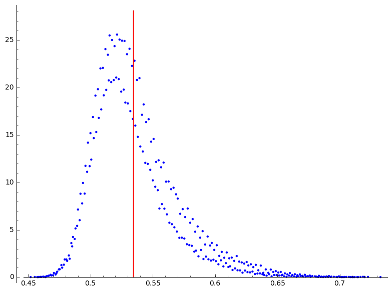
$n=10$:
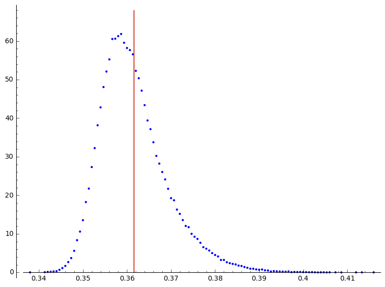
$n=11$:

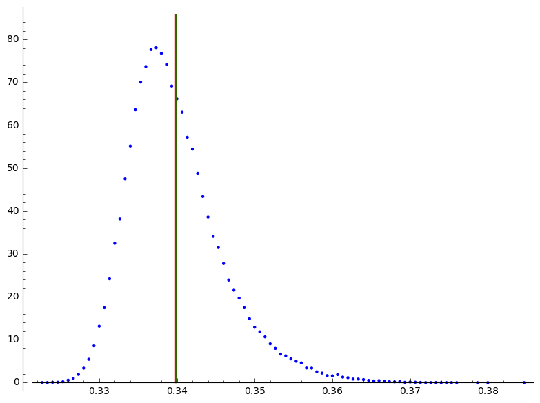
Figure 5: Empirical density of $X_{n}$ for $K=\mathbb{Q}_{2}$ and $d=2$

$n=3$:
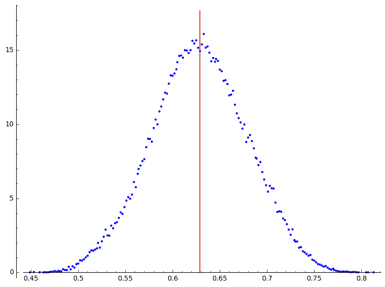
$n=8$:
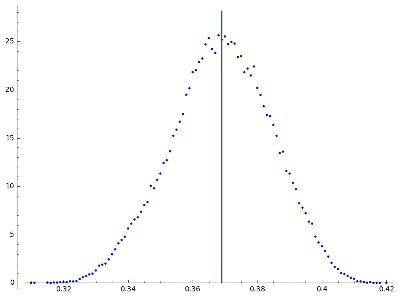
$n=9$:

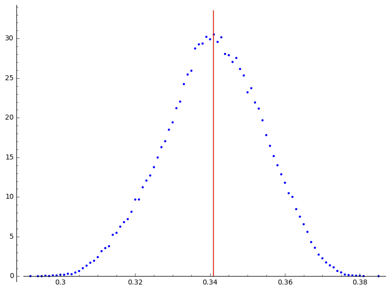
Figure 6: Empirical density of $X_{n}$ for $K=\mathbb{Q}_{2}$ and $d=3$

Going further one can draw the empirical “density”: we subdivise $\mathbb{R}$ into small intervals and count, for each of them, the proportion of sample points (renormalized by the size of the interval) leading to a point in it. The results are displayed in Figure 5 (page 5) and Figure 6 (page 6) in dimension $2$ and $3$ respectively. The red and green vertical lines (which actually always collapse) in these pictures indicate the theoretical mean and the empirical mean of $X_{n}$ respectively.

For a fixed dimension, the density curves (for various $n$) all have a similar shape. This may suggest that the law of $X_{n}$ — correctly renormalized — converges to some limit. We believe that it would be very interesting to investigate further this question. For example if one can compute this limit and check that it is zero until some point, it would eventually imply the Kakeya conjecture for almost all non-archimedean Kakeya sets.

We finally remark that, on the first diagram of Figure 5, one can clearly separate two curves. This reflects a parity phenomenon: $q^{nd}X_{n}=2^{10}X_{5}$ is even with probability $\approx 73\%$ and odd with probability $\approx 27\%$. The curve below then corresponds to odd values of $X_{5}$ while the curve above corresponds to even values. This phenomenon tends to disappear rapidly when $n$ grows up.

4.2 Visualizing a random $2$-adic Kakeya set

In order to draw a $2$-adic Kakeya set sitting naturally in $\mathbb{Z}_{2}^{d}$, we will necessarily need to relate $\mathbb{Z}_{2}$ and $\mathbb{R}$. In order to do so, we use the “reverse” function $r:\mathbb{Z}_{2}\to[0,1]$ mapping the $2$-adic integer $\sum_{i=0}^{\infty}2^{i}s_{i}$ (with $s_{i}\in\{0,1\})$ to the real number $\sum_{i=0}^{\infty}2^{-i-1}s_{i}$.

Note that $r$ is continuous (it is actually $1$-Lipschitz) but not injective since the binary representation of a real number fails to be unique in general. For instance $\frac{1}{2}$ has two preimages which are $1\in\mathbb{Z}_{2}$ and $-2\in\mathbb{Z}_{2}$. The closed intervals $[0,\frac{1}{2}]$ and $[\frac{1}{2},1]$ correspond to the disjoint cosets $2\mathbb{Z}_{2}$ and $2\mathbb{Z}_{2}+1$ respectively. Note that the latter are open and closed in $\mathbb{Z}_{2}$. More generally all real number of the form $\frac{a}{2^{n}}$ have two distinct preimages in $\mathbb{Z}_{2}$ and there always exist two closed interval meeting $\frac{a}{2^{n}}$ corresponding to two open closed subsets of $\mathbb{Z}_{2}$.

Remark 4.1.

There actually exist closed embeddings $\mathbb{Z}_{2}\to\mathbb{R}$; an example of it is the Cantor mapping $C$ taking $\sum_{i=0}^{\infty}2^{i}s_{i}\in\mathbb{Z}_{2}$ to $2\cdot\sum_{i=0}^{\infty}3^{-i-1}s_{i}$. The image of $C$ is the usual triadic Cantor set and $C$ induces an homeomorphism between it and $\mathbb{Z}_{2}$. We nevertheless preferred to use $r$ because it maps $\mathbb{Z}_{2}$ to an interval whereas $C$ maps $\mathbb{Z}_{2}$ to a null set. Working with $C$ has then two disadvantages: it would lead to undrawable pictures on the one hand and would not reflect properly the properties we want to emphasize on the other hand.

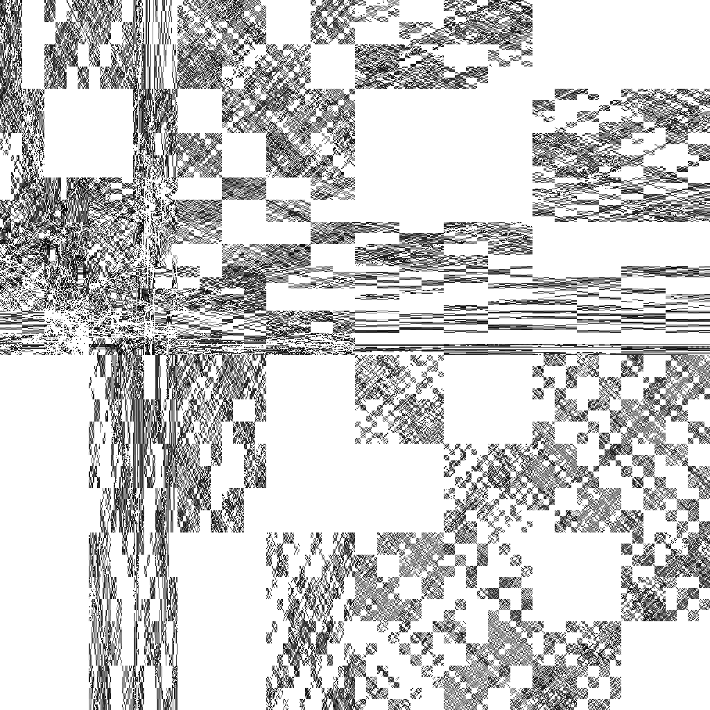
Figure 7: A $2$-dimensional random Kakeya set over $\mathbb{Q}_{2}$

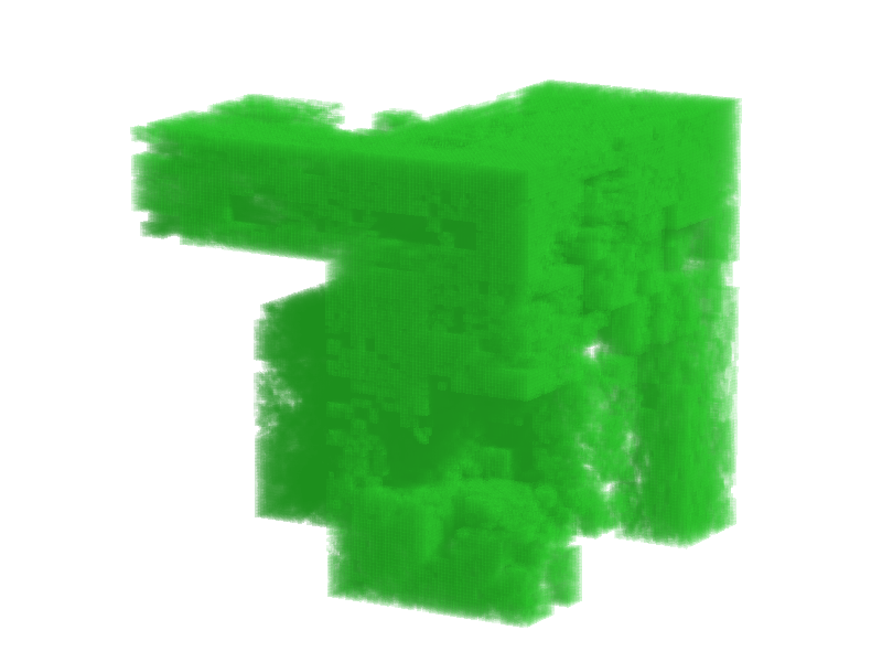
Figure 8: A $3$-dimensional random Kakeya set over $\mathbb{Q}_{2}$

Viewing $\mathbb{Z}_{2}^{2}$ in $\mathbb{R}^{2}$ through the map $(r,r)$, the picture of Figure 7 (page 7) represents a random Kakeya set — or more precisely its $(2^{-13})$-neighbourhood — in $\mathbb{Z}_{2}^{2}$. An animation showing a $2$-adic needle moving continuously in the $2$-adic plane and filling a $2$-adic Kakeya set is available at the URL:

http://xavier.toonywood.org/papers/publis/kakeya/kakeya-2d.gif

Finally, a $3$-dimensional $2$-adic Kakeya set is displayed on Figure 8 and a movie showing it on different angles can be found at:

http://xavier.toonywood.org/papers/publis/kakeya/kakeya-3d.mp4

Appendix A Appendix: Discrete valuation fields

This appendix is dedicated to readers who are not familiar with non-archimedean geometry. It presents a quick summary of the most important basic definitions and facts of the domain. All the material presented below is very classical.

Definitions

A discrete valuation field is a field $K$ equipped with a map $\text{\rm val}:K\to\mathbb{Z}\cup\{+\infty\}$ (the so-called valuation) satisfying the following axioms:

1. $\text{\rm val}(x)=+\infty$ if and only if $x=0$,

2. $\text{\rm val}(xy)=\text{\rm val}(x)+\text{\rm val}(y)$,

3. $\text{\rm val}(x+y)\geqslant\min(\text{\rm val}(x),\text{\rm val}(y))$

for all $x$ and $y$ in $K$. The valuation val is non trivial if there exists an element $x\in K^{\star}$ with $\text{\rm val}(x)\neq 0$. Under this additional assumption, the set $\text{\rm val}(K^{\star})$ is a subgroup of $\mathbb{Z}$ and therefore is equal to $n\mathbb{Z}$ for some positive integer $n$. An element $\pi\in K$ of valuation $n$ is called a uniformizer of $K$. One can always renormalize the valuation (by dividing it by $n$) in order to ensure $n=1$.

The valuation on $K$ readily defines a family of absolute values $|{\cdot}|_{a}$ ($a>1$) on $K$ by:

$$\forall a\in(1,\infty),\,\forall x\in K,\quad|x|_{a}=a^{-\text{\rm val}(x)}$$

with the convention that $a^{-\infty}=0$. Each of these absolute values defines a distance $d_{a}$ on $K$ by the usual formula $d_{a}(x,y)=|x-y|_{a}$. It is easily seen that all these distances define the same topology on $K$. We underline that $d_{a}$ is ultrametric in the sense that:

$$\forall x,y,z\in K,\qquad d_{a}(x,z)\leqslant\max\big{(}d_{a}(x,y),d_{a}(y,z)\big{)}.$$ (22)

This stronger version of the triangle inequalities has unexpected and important consequences. For instance it implies that $d_{a}(x,z)=\max\big{(}d_{a}(x,y),d_{a}(y,z)\big{)}$ as soon as $d_{a}(x,y)\neq d_{a}(y,z)$, showing then that every triangle in $K$ is isosceles. Similarly if two balls $B_{1}$ and $B_{2}$ of $K$ meet, we necessarily have $B_{1}\subset B_{2}$ or $B_{2}\subset B_{1}$.

Let $R$ be the closed unit ball of $K$ (this does not depend on the parameter $a$); alternatively $R$ is the subset of $K$ consisting of elements $x$ with nonnegative valuation. An important remark following from axioms (ii) and (iii) is that $R$ is a subring of $K$; it is usually called the ring of integers of $K$. The invertible elements in $R$ are clearly exactly the elements of norm $1$ (since the norm is multiplicative). On the contrary, the open unit ball $\mathfrak{m}$ is an ideal of $R$. It is actually the unique maximal ideal of $R$ (showing that $R$ is a local ring). It is moreover principal and generated by any uniformizer of $K$. The quotient $k=R/\mathfrak{m}$ is a field which is called the residue field of $K$.

Examples

1. Let $p$ be a prime number. Recall that the $p$-adic valuation of a nonzero integer $n$ is defined as the greatest integer $v$ such that $p^{v}$ divides $n$; it is often denoted by $v_{p}(n)$. This construction defines a function $v_{p}:\mathbb{Z}\backslash\{0\}\to\mathbb{N}$. We extend it to a function $\mathbb{Q}\to\mathbb{Z}\cup\{+\infty\}$ by setting:

$$v_{p}(0)=+\infty\quad\text{and}\quad\textstyle v_{p}(\frac{a}{b})=v_{p}(a)-v_{p}(b)$$

for $a,b\in\mathbb{Z}$. One checks that $v_{p}$ satisfies the axioms of a valuation, turning then $\mathbb{Q}$ into a discrete valuation field. A uniformizer of $(\mathbb{Q},v_{p})$ is $p$. Its rings of integers is the ring $\mathbb{Z}_{(p)}$ consisting of fractions $\frac{a}{b}$ where $b$ is not divisible by $p$. Its residue field is isomorphic to $\mathbb{Z}/p\mathbb{Z}$.

2. Let $k$ be any field and $K=k(t)$ be the field of univariate rational fractions over $k$. Given $f\in K$, $f\neq 0$, let $\text{\rm ord}(f)$ denote the order of vanishing of $f$ at $0$, i.e. $\text{\rm ord}(f)$ is the unique integer for which one can write $f=t^{\text{\rm ord}(f)}\cdot g$ where $g\in k(t)$ is defined and does not vanish at $0$. This defines a function $\text{\rm ord}:K^{\star}\to\mathbb{Z}$ that we extend to $K$ by letting $\text{\rm ord}(0)=+\infty$. One then checks that $(K,\text{\rm ord})$ is a discrete valuation field. Its ring of integers consists of fractions $\frac{f}{g}$ where $f$ and $g$ are polynomials with $g(0)\neq 0$. A uniformizer of $(K,\text{\rm ord})$ is $t$ and its residue field is canonically isomorphic to $k$.

Completeness

A discrete valuation field $(K,\text{\rm val})$ is said complete is it complete with respect to one (or equivalently all) $d_{a}$. Using the ultrametric triangle inequality (22), we easily check that, assuming that $K$ is complete, a series $\sum_{n\geqslant 0}u_{n}$ (with $u_{n}\in K$) converges if and only if the sequence $(u_{n})_{n\geqslant 0}$ converges to $0$.

Let $(K,\text{\rm val})$ be a discrete valuation field and let $\hat{K}_{a}$ be the completion of the metric space $(K,d_{a})$. One checks that $\hat{K}_{a}$ does not depend on $a$, so that we can denote it safely simply $\hat{K}$. Observe that the ring operations extend uniquely to $\hat{K}$, turning then it into a field. Similarly the continuous map $\text{\rm val}:K\to\mathbb{Z}\cup\{+\infty\}$ extends uniquely to $\hat{K}$, turning then $\hat{K}$ into a discrete valuation field. By construction $\hat{K}$ is moreover complete. The ring of integers $\hat{R}$ of $\hat{K}$ can be seen as the completion of $R$ or, alternatively, as the topological closure of $R$ in $\hat{K}$. Note moreover that a uniformizer of $K$ remains a uniformizer of $\hat{K}$ (since the valuation on $\hat{K}$ extends that on $K$) and that the residue field of $\hat{K}$ is canonical isomorphic to that of $K$.

Elements in complete discrete valuation fields can be explicitely described as the values at a fixed uniformizer of particular power series.

Proposition A.1.

Let $K$ be a complete discrete valuation field. Let $R$ be its ring of integers, $k$ be its residue field and $\pi$ be a fixed uniformizer. Let $S\subset R$ be a fixed complete system of representatives of $k$ and assume $0\in S$. Then:

1. any element $x\in R$ can be written uniquely as a converging sum:

   $$x=s_{0}+s_{1}\pi+s_{2}\pi^{2}+\cdots+s_{n}\pi^{n}+\cdots$$ (23)

   with $s_{n}\in S$ for all $n\geqslant 0$

2. any element $x\in K$ can be written uniquely as a converging sum:

   $$x=s_{v}\pi^{v}+s_{v+1}\pi^{v+1}+s_{v+2}\pi^{v+2}+\cdots+s_{n}\pi^{n}$$

   with $v\in\mathbb{Z}$, $s_{n}\in S$ for all $n\geqslant v$. We can moreover require that $s_{v}\neq 0$, in which case we have $v=\text{\rm val}(x)$.

Proof.

We only prove the first statement, the second being totally similar. We first remark that the series (23) converges since its general term $s_{n}\pi^{n}$ goes to $0$ when $n$ goes to infinity.

Assume first that we are given a decomposition (23). Then $s_{0}$ has to be congruent to $x$ modulo $\pi$ and therefore is uniquely determined since $S$ is by definition a complete set of representatives of $k=R/\pi R$. Substrating $s_{0}$, dividing by $\pi$ and applying the same reasoning, we find that $s_{1}$ is uniquely determined as well. Repeating this argument again and again, we get the unicity of the decomposition (23).

Now pick $x\in R$. Define $s_{0}$ as the unique element of $S$ which is congruent to $x$ modulo $\pi$. Then $r_{1}=\frac{x-s_{0}}{\pi}$ lies in $R$. We can thus repeat the construction and define $s_{1}$ as the unique element of $S$ which is congruent to $r_{1}$ modulo $\pi$. We construct this way an infinite sequence $(s_{n})_{n\geqslant 0}$ of elements of $S$ with the property that $x\equiv s_{0}+s_{1}\pi+s_{2}\pi^{2}+\cdots+s_{n-1}\pi^{n-1}\pmod{\pi^{n}}$ for all $n$. Passing to the limit (and noting that $\pi^{n}$ goes to $0$), we get (23). ∎

Examples

1. The field $\mathbb{Q}$ equipped with the $p$-adic valuation $v_{p}$ is not complete. Its completion is the field of $p$-adic numbers $\mathbb{Q}_{p}$. A uniformizer of $\mathbb{Q}_{p}$ is $p$ and its residue field is $\mathbb{Z}/p\mathbb{Z}$. The ring of integers of $\mathbb{Q}_{p}$ is usually denoted by $\mathbb{Z}_{p}$; its elements are the so-called $p$-adic integers. According to Proposition A.1, any $p$-adic integer can be uniquely written as a sum:

$$s_{0}+s_{1}p+s_{2}p^{2}+\cdots+s_{n}p^{n}+\cdots$$

with $s_{n}\in\{0,1,\ldots,p{-}1\}$. It is the decomposition in $p$-basis of a $p$-adic integer.

2. Similarly, the field $k(t)$ equipped with the valuation ord is not complete. Thanks to Proposition A.1, its completion consists of series of the shape:

$$s_{v}t^{v}+s_{v+1}t^{v+1}+s_{v+2}t^{v+2}+\cdots+s_{n}t^{n}+\cdots$$

with $v\in\mathbb{Z}$ and $s_{n}\in k$. It is therefore nothing but the field of univariate Laurent series over $k$, usually referred to as $k((t))$. Its rings of integers is the ring of power series over $k$, namely $k[[t]]$. Again its rings of integers is canonically isomorphic to $k$.

The Haar measure

Let $(K,\text{\rm val})$ be a complete discrete valuation ring with ring of integers $R$ and residue field $k$. From now and until the end of this appendix, we assume that $k$ is finite.

The first part of Proposition A.1 shows that $R$ is homeomorphic to $k^{\mathbb{N}}$ (i.e. the set of all sequences with coefficients in $k$) and therefore is compact. Since $R$ carries in addition a group structure, it is endowed with a unique Haar measure $\mu$ normalized by $\mu(R)=1$. This measure extends uniquely to a Haar measure on $K$. Be careful nevertheless that $\mu(K)$ is infinite.

Under the additional assumptions of this paragraph, it is quite convenient to normalize the norm $|\cdot|$ on $K$ by $|\pi|=\frac{1}{\text{\rm Card}\>k}$ where $\pi$ is any uniformizer. (If the valuation is normalized so that it takes the value $1$, the above norm is the norm $|\cdot|_{\text{\rm Card}\>k}$ we have introduced before.) The above convention leads to the expected relation:

$$\mu(aE+b)=|a|\cdot\mu(E)$$

for all $a,b\in K$ and all measurable subset $E$ of $K$ (and where $aE+b$ denotes of course the image of $E$ under the affine transformation $x\mapsto ax+b$).

References

- [1] Y. Babichenko, Y. Peres, R. Peretz, P. Sousi, P. Winkler, Hunter, Cauchy Rabbit, and Optimal Kakeya Sets, Trans. Amer. Math. Soc. 366 (2014), 5567–5586
- [2] A. Besicovitch, On Kakeya’s problem and a similar one, Math. Z. 27 (1928), 312–320
- [3] E. Dummit, M. Hablicsek, Kakeya sets over non-archimedean local rings, Mathematika 59 (2013), 257–266
- [4] Z. Dvir, On the size of Kakeya sets in finite fields, J. Amer. Math. Soc. 22 (2009), 1093–1097
- [5] J. Ellenberg, R. Oberlin, T. Tao, The Kakeya set and maximal conjectures for algebraic varieties over finite fields, Mathematika 56 (2010), 1–25
- [6] R. Fraser, Kakeya-Type Sets in Local Fields with Finite Residue Field, Mathematika 62 (2016), 614–629
- [7] B. Green, Restriction and Kakeya Phenomena, lecture notes from a course at Cambridge, http://people.maths.ox.ac.uk/greenbj/papers/rkp.pdf
- [8] N. Katz, T. Tao, New bounds for Kakeya problems, J. Anal. Math. 87 (2002), 231–263
- [9] T. Wolff, An improved bound for Kakeya type maximal functions, Rev. Mat. Iberoamericana 11 (1995), 651–674
- [10] T. Wolff, Recent work connected with the Kakeya problem, in Prospects in mathematics (Princeton, NJ, 1996), pp. 129–162, Amer. Math. Soc., Providence, RI (1999)