Convergence of Newton’s method in shape optimisation via approximate normal functions
Abstract
In this paper we propose a Newton method for shape functions defined on an image set generated by the (Micheletti) metric group. We review basic properties of the metric group and a quotient associated with the metric group and a fixed domain.
Taking into account the special structure of the second shape derivative and its symmetric part allows us to distinguish between two Hessians, the domain shape Hessian and the boundary shape Hessian.
Using the domain Hessian we define a Newton method on the metric group by discretising the tangent space of the quotient via approximate normal functions using reproducing kernels. Under suitable assumptions we are able to show superlinear convergences of the Newton iterations and additionally convergence of the shapes in the metric group. Finally we verify our findings in a number of numerical experiments including a thorough numerical study of the impact of the discretisation on the convergence speed.
Keywords: shape optimization, Micheletti group, Newton methods, convergence analysis, numerical mathematics
Introduction
Shape optimisation is concerned with the minimisation of real-valued shape functions over an admissible set containing a collection of subsets ; see [20, 37, 8, 19]. Many tasks and processes in industry can be optimised using shape optimisation methods. Therefore it is of paramount importance to find efficient methods to solve these problems numerically.
The aim of this paper is to develop a Newton algorithm to find stationary points of shape functions defined on an image set generated by the metric group ; cf [8, Chapter 3] and [26, 18]. For every fixed set the image set consists of all images , where belongs to the metric group . This image set can be identified with the quotient that identifies transformations in with the same image on . Using the special structure of the second Euler derivative and its symmetric part allows us to define two shape Hessians, the domain (shape) Hessian and the boundary (shape) Hessian. The domain and boundary Hessian are functions defined on the tangent space of the metric group and its quotient space, respectively, and coincide when they are restricted to normal perturbations on the boundary. We also establish a new proof of the structure theorem for the symmetric part of the second Euler derivative; [30, 4].
In order to approximate the Newton equation we need to approximate the tangent space or a subspace of in a suitable way. For this purpose we introduce for every submanifold of co-dimension one (having in mind ) so called approximate normal functions. The properties of the reproducing kernel ensure that these functions are linearly independent. Additionally approximate normal functions are approximately normal along and thus are suitable functions to approximate a subset of the tangent space of the quotient space . In order to have a sparse Hessian approximation we work with compactly supported reproducing kernels. A key ingredient of the proof is a transport that relates approximate normal functions on different domains. This allows us to show superlinear convergence of Newton’s method in the discrete setting. Our analysis reveals that quadratic convergence cannot be expected when normal fields are approximated.
Second order methods such as Newton and Newton-like methods have the great advantage over gradient methods that they converge superlinearly or even quadratically. Despite their importance, the literature on second order methods for shape optimisation problems is incomplete and only a limited number of papers use second order information; see [12, 13, 21, 22, 15, 14, 2, 31, 33]. Convergence analysis of second order methods is even less studied; [34, 22, 16].
One reason for the lack of literature in this field is the notorious nonlinearity of the space of admissible shapes which leads to nonconvex optimisation problems. However in some situations it is possible to turn admissible sets into a (mostly Riemannian) manifold and therefore tools from differential geometry become accessible. Newton methods, Newton-like and gradient methods on finite dimensional Riemannian manifolds were already subject of intensive research [1, 32]. In shape optimisation the spaces of shapes are at best infinite dimensional manifolds and in this situation the analysis is more complicated as one has to account for the infinite dimensionality of the manifold; [23, 27]. In the recent work [34] the link between shape optimisation problems and a certain infinite dimensional Riemannian manifolds of mappings, also called shape space, has been established. To be more specific the analysis was carried out in the so-called shape space of plane curves studied in [28]. In this paper we want to provide another approach employing the Micheletti metric space.
Structure of the paper
In Section 1 we recall the definition of the
metric group and its basic properties.
In Section 2, we recall the structure of first and second shape derivatives. We give a new proof of the structure of the symmetric part of the second derivative (referred to as third structure theorem). Then we introduce two shape Hessians, the domain shape Hessian and boundary shape Hessian defined on the tangent space of and , respectively.
In Section 3, we use reproducing kernels to introduce novel approximate normal basis functions. These functions yield an approximation of subspace of the tangent space of the quotient . It turns out that the domain and boundary shape Hessian restricted to the space of approximate normal functions are approximately the same. As a result as long as we are close to a stationary point we can use the domain Hessian instead of the boundary Hessian.
In Section 4, we introduce and study a Newton method using the approximate normal functions from Section 3. A careful analysis shows that, under suitable conditions, the Newton method converges superlinear. The generated transformations which correspond to the shapes convergence in the metric of .
Section 6 provides some numerical results comparing a gradient method with Newton’s methods defined by different Hessians. We show experiments employing the domain, boundary and Riemannian shape Hessian [34]. These results are compared with a standard gradient algorithm and show the superiority of Newton’s method near a stationary point.
1 Micheletti’s metric group and its properties
This section builds the basis upon which we will develop our Newton method and its convergence proof. Particularly we introduce function spaces, define the Micheletti metric group, and recall some of its properties.
1.1 Function spaces
Throughout this paper is an open set. We denote the space of continuous vector fields on vanishing on by
We denote by , , the usual space of -times continuously differentiable functions on with values in . The space comprises all functions from that admit a uniformly continuous and bounded extensions of its partial derivatives to for all multi-indices satisfying . The space indicates all -times differentiable functions on with values in that have bounded and continuous partial derivatives for all multi-indices . We equip the spaces and with the norm where denotes the first derivative of .
For all spaces introduced above we define subspaces: and . It is worth nothing that .
The flow of a vector field is defined by for and , where is the solution of , and ; see [6, pp. 131].
1.2 Group of transformations and metric
We begin with the definition of the metric group and review some of its basic properties; see [8, Chapter 3].
Definition 1.1 ([8, p.124]).
The Micheletti group associated with the Banach space is defined by
| (1.1) |
This set is a group under composition . The transformations in are unbounded, since the identity mapping on is unbounded and is bounded. However, their derivative is bounded since the identity matrix and are both bounded on .
Definition 1.2 ([8, p.126]).
The distance between the identity mapping on and is defined by
| (1.2) |
The distance between arbitrary is defined by
It is readily checked that is right-invariant, that is, for all . The symmetry follows from the right-invariance and the definition of the metric. For a proof that satisfies the triangle inequality and the completeness of we refer to [8, p.134, Theorem 2.6].
1.3 Image sets and subgroup
In shape optimisation the metric space is used as follows. We take an arbitrary set and associate with it the image set
| (1.3) |
This set forms the set of all admissible shapes on which a shape function is to be minimised. In the following sections we study a Newton method that aims to find stationary points of a shape function .
A set does not correspond to a unique as two elements can have the same image . Therefore we identify transformations whose image coincides on . For this purpose we define a subgroup of by
| (1.4) |
It is readily checked that is a subgroup of and hence the quotient is well-defined. It can also be shown that equipped with the quotient metric is a complete metric space ([8, Theorem 2.8, p. 141]) itself if for example is a smooth domain or open and crack free (); see [8, Chapter 3]. Henceforth we denote the equivalence classes of by .
Definition 1.3.
The set and the quotient are identified via the bijection that maps the equivalence class to its images . Every function is identified with via
1.4 Properties of the metric
Let us now extract some refined properties of the metric . These properties are used later for the proof of our Newton method. We show that if the norm of is smaller than one, then the distance can be estimated from above.
Lemma 1.4.
Let be arbitrary. For all such that , we have
| (1.5) |
Particularly with .
Proof.
Firstly by definition of as an infimum, for all . As is a bijection, we have . By the chain rule we obtain and thus using again that is a bijection gives
| (1.6) |
Let denote the inverse mapping defined for all invertible . For given invertible and with , we get by [3, Satz 7.2] the Lipschitz estimate . It follows by the triangle inequality Hence setting and for fixed yields Thus using this estimate in (1.6) we arrive at and this finishes the proof. ∎
The next lemma shows a statement similar to Lemma 1.4, but without the assumption that the norms of being smaller than one. However, the estimate is not as sharp. We also refer to [8, p. 127, Example 2.2] where the Banach space of bounded Lipschitz continuous functions rather than is considered.
Lemma 1.5.
For all in , , we have
| (1.7) |
Proof.
The proof follows the lines of [8, p. 127, Example 2.2] and is therefore deferred to the appendix. ∎
With the help of the previous lemma we can show that the convergence of to in implies the convergence of and to and in , respectively. This statement is summarised in the following lemma.
Lemma 1.6.
Let be given and assume in as . Then
| (1.8) |
Proof.
Thanks to the right invariance of metric we have . Therefore we may assume without loss of generality that and and in . By assumption for every we find such that for all . By definition of as an infimum we find for every number , a number and transformations such that and
| (1.9) |
Now Lemma 1.5 yields for all . Since was arbitrary we conclude as . Noticing as shows that the argumentation above can be repeated to prove as which finishes the proof. ∎
1.5 Parametrisations of
In the following lemma denotes the open ball in with radius centered at the origin.
Lemma 1.7.
Let be arbitrary. For each the mapping
| (1.10) |
, is a well-defined parameterisation of a neighborhood of . Differentiable charts are given by with . Additionally, the sets are open in .
Proof.
We first show that for given the mapping
| (1.11) |
is well-defined when we choose . Indeed we can write . By the choice of we have and hence [8, Theorem 2.14, (i), p.148] implies that the chart is well-defined.
Next we show that the chart change is smooth. Let be given. The chart change is given by
| (1.12) |
which is obviously . Recall that denotes the open ball of radius at the origin in .
It remains to show that is indeed open. Let , be given. Notice that by definition of the set we have . Therefore is positive. Let be arbitrary. We need to show that there is , such that for all with . Let be any element satisfying . The fact that is a homeomorphism gives us The definition of and Lemma 1.5 (as in the proof of Lemma 1.6) yield
| (1.13) |
Therefore we can choose so small that . Then
| (1.14) |
and similarly by choosing so small that we achieve the estimate,
| (1.15) |
We conclude that if is so small that , then the -ball around in the -topology is contained in and hence is open in . ∎
2 Structure of first and second derivatives and shape Hessians
This section is devoted to the structure of first and second order derivatives that were previously studied in [44, 24, 36, 4, 7]. First we recall structure theorems giving the structure of the first and second derivative. Then we turn our attention to the structure of the symmetric part of the second derivative as it is of great importance for our Newton method; [30]. We present a new proof of the structure theorem of the symmetric part by a successive application of the first and second structure theorem. The novelty of our approach is to connect all structure theorems with each other.
2.1 Definition of first and second derivatives
The following definition recalls the standard notion of derivative of shape functions using the perturbation of identity. For given set we denote by the powerset of . We restrict ourselves to shape functions defined on , where was defined in (1.3). Notice that if is only of class , then the elements in are only of class . However, we sometimes assume that a set in is more regular for in which case we silently assume that is more regular.
In this section let be a bounded domain.
Definition 2.1.
Let be a shape function and take . Let be two vector fields.
-
(i)
The directional derivative of at in direction is defined by
(2.1) -
(ii)
The second directional derivative of at in direction is defined by
(2.2) ( exists for all small ).
-
(iii)
If the directional derivative exists for all small , then the second Euler derivative of at in direction is defined by
(2.3)
The following definition is concerned with the shape differentiability which we define as Hadamard semi-differentiability; see [8, pp. 471].
Definition 2.2.
Let be a shape function and let .
-
(i)
We say that is differentiable at if
(2.4) exists for all and is linear and continuous on .
-
(ii)
We say is twice differentiable at if it is differentiable in a neighborhood of , and if
-
the mapping is continuous at all .
-
for all the limit
(2.5) exists, is bi-linear and continuous on .
-
Recall that denotes the flow of a vector field .
Lemma 2.3.
Assume that is differentiable at . Then we have
| (2.6) |
for all .
Proof.
Setting we can write . Since in as , we obtain
| (2.7) |
∎
Lemma 2.4.
Let be differentiable at and assume that is of class . Then
| (2.8) |
where denotes the outward pointing unit normal vector field along .
Proof.
Example 2.5.
As an illustration of the previous definition consider where is bounded and open. This example can be found in [38, pp. 28–29 ,Example 2.37]. If , then is differentiable at with derivative in direction given by
| (2.9) |
Here denotes the inner product on the space of matrices defined for by Notice that for all small and ,
| (2.10) |
As a result if belongs to , then is twice differentiable at with derivative
where and , Notice that exists for all and is given This decomposition of the Euler derivative is well-known (see [36]) and holds for all twice differentiable shape functions . We recall the precise statement in Lemma 2.9.
2.2 Quotient space and restriction mapping
Let be an integer. We introduce an equivalence relation on as follows: two vector fields are equivalent, written , if and only if on . In other words two vector fields are equivalent if their restriction ot coincides. We denote the set of equivalence classes and its elements by and , respectively. We denote by the restriction mapping of vector field belonging to to mappings , that is, where denotes the space of all mappings from into . The mapping induces the mapping and by definition , where denotes the canonical surjection mapping a vector field to its equivalence class in . We denote by the image of .
2.3 First structure theorem
The following theorem provides the structure of the first (shape) derivative of a shape function .
Theorem 2.6.
Let be given and assume that is differentiable at . Then:
-
(i)
There is a linear mapping such that
(2.11) for all .
-
(ii)
If , then and is a continuous functional.
-
(iii)
If , then is continuous on and satisfies
(2.12)
2.4 Second structure theorem
In this section we recall the second structure theorem that provides a structure of . For more information we refer to [4, 30] and [8, pp. 501].
Lemma 2.7.
Let and be given. Assume that is twice continuously differentiable on . Then
| (2.13) |
Proof.
This is a consequence of Schwarz’s theorem. Particularly is twice continuously differentiable on . ∎
Remark 2.8.
If the function , defined in Lemma 2.7, is not twice continuously differentiable, then may be nonsymmetric. Consider for instance with only twice differentiable on . Then is not necessarily symmetric which may destroys the symmetry of .
The following theorem is called second structure theorem as it provides the structure of which was first observed in [36].
Theorem 2.9.
Assume that is twice differentiable at the open set . Then we have for all and ,
| (2.14) |
and
| (2.15) |
2.5 Third structure theorem and a new proof
The structure of the symmetric part of the second derivative was already analysed in [30]. The novelty of our approach lies in the way how we derive it. We deduce the structure of the symmetric part by successively applying the first and second structure theorem.
Notation
In the following we use the notation and to indicate the tangential part of the vector fields and restricted to . Here is the outward pointing unit normal field along and denotes the tensor product defined by for all . The tangential gradient of and Jacobian and divergence of can then be defined by , and , where are extensions of to a neighborhood of
Third structure theorem
The following theorem will be referred to as third structure theorem.
Theorem 2.10.
Let be an open set and let be twice differentiable at .
-
(i)
There are mappings and , such that
(2.16) and hence
(2.17) for all .
-
(ii)
If , then and and are continuous on .
-
(iii)
If , then and are continuous on and , respectively and satisfy
(2.18) for all .
Proof.
(i): Firstly on account of the differentiability assumption on and of Theorem 2.9 we have for all and . Let and . The Banach fixed point theorem shows that is bijective on for all small enough. Moreover if on , then for all small . Thus we have for all and with on and by density this yields for all with on . Hence the mapping is well-defined for all . Since is a bijection onto , we can define which satisfies by definition
| (2.19) |
for all . Finally by
the first structure theorem (Theorem 2.6), we have
for all
and plugging this together with (2.19) into (2.14) we recover (2.17) and also (2.16).
(ii) This follows from the continuity of the extension operator .
(iii)
Note that since is , Theorem 2.6 item (iii) yields that
is continuous on and
satisfies
for all .
It follows from Lemma 2.4 that for all with on
. In view of (2.17) this yields for all with on
. Since this is equivalent to the important equation
| (2.20) |
Now let be arbitrary. Splitting the restrictions of to into normal and tangential parts and inserting the results into (2.20) gives
| (2.21) |
valid for all . Now notice that and hence
| (2.22) |
and by interchanging the roles of and also
| (2.23) |
Since on we get on . Multiplying with any tangent vector yields . This means and hence . Therefore inserting (2.22),(2.23) into (2.21) gives us
| (2.24) |
Finally setting we recover formula (2.18). ∎
2.6 Boundary and domain Hessian
Definition the shape Hessians
We now define a two shape Hessians.
Definition 2.12.
Let be given and assume that is twice differentiable at . The domain shape Hessian of at is defined by
| (2.27) |
Let be a -extension of the outward pointing unit normal field along and set . The boundary shape Hessian at is defined by
| (2.28) |
for all .
Remark 2.13.
-
(i)
Within our framework both Hessians are symmetric. For functions defined on the domain Hessian corresponds to the Hessian on the manifold . It only depends on the Euclidean connection . The canonical Hessian on the quotient is the boundary Hessian, which only depends on the Euclidean connection.
-
(ii)
Our approach is based on the metric group associated with the vector space . However, other vector spaces to construct a metric group, e.g. the space of bounded and Lipschitz continuous function , are possible. Since the metric group is contained in an affine space , where equals e.g. or , the tangent space of the corresponding metric group is always ; see [9, Theorem 2.17, p.151].
The boundary Hessian is defined as the restriction of the domain Hessian to normal perturbations. Hence we have for all with on . Moreover if satisfies the assumptions of Theorem 2.10, then
Example of boundary and domain shape Hessians
Let us briefly revisit the shape function , where and is open and bounded. In Example 2.5 we computed the domain shape Hessian of , namely
| (2.29) |
where and and Following the steps of the proof of [25, Lemma 3.11] we can readily bring (2.29) into the boundary form (2.18). Since for all with , we conclude by partial integration everywhere in . This in turn shows by partial integration for all . Recall that , where is the mean curvature of . Then by splitting the restrictions of to into normal and tangential part and assuming is of class we check,
| (2.30) |
Using the tangential Stokes formula [8, p.498] we obtain
| (2.31) |
Further by splitting into normal and tangential part,
| (2.32) |
Plugging (2.31) and (2.32) into (2.30) and using we obtain
| (2.33) |
Notice that (2.30) has the predicted form (2.18). From (2.30) we also see that the boundary shape Hessian is given by
| (2.34) |
Remark 2.14 (Positive definiteness).
As a conclusion of the previous example we see that the boundary Hessian of will be positive definite if on for some constant . Then for all . However, the boundary Hessian does not need to be positive definite in a stationary point . Indeed consider given by
| (2.35) |
Then is a stationary point of , but also the second derivative vanishes at .
2.7 Newton’s equation on and
Let be a twice differentiable shape function on and take any .
Definition 2.15.
We call a domain Newton direction at if and , solves
| (2.36) |
We call a boundary Newton direction at if
| (2.37) |
The task of the next section is to construct a finite dimensional subspace of on which (2.36) can be solved.
3 Approximate normal basis functions
This section is devoted to the construction of basis functions, called approximate normal functions, with which we aim to discretise the Newton equation (2.36). The idea is to construct vector fields that are linearly independent and additionally ”normal enough” to domain of interest such that the discrete Hessians can be inverted.
The main ingredient for our construction are symmetric positive definite kernels and more specifically positive definite radial kernels. Positive definite and symmetric kernels generate reproducing kernel Hilbert spaces (RKHS) which are characterised by the property that the point evaluation is a continuous functional. They allow to work with the reproducing kernel instead of the RKHS itself. For instance shape gradients may be computed explicitly as shown in [11] without solving a boundary value problem
Throughout this section is a -submanifold of codimension one and we denote by a normal field along .
3.1 Reproducing kernel Hilbert spaces
We begin with the definition of matrix-valued reproducing kernels.
Definition 3.1.
Let be an arbitrary set. A function is called matrix-valued reproducing kernel for the Hilbert space of functions , if for all and ,
In case we call scalar reproducing kernel and in order to distinguish the matrix and scalar case we set and .
Remark 3.2.
-
•
Notice that in case the items (a) and (b) of the previous definition read: for all and we have , and
-
•
Notice that items (a) and (b) together imply that the point evaluation is a continuous functional on a reproducing kernel Hilbert space.
The following remark collects a few interesting properties of reproducing Hilbert spaces; cf.[42].
Remark 3.3.
-
•
It is readily checked that a (scalar) reproducing kernel is symmetric, for all . It is also positive semi-definite, that is, for all mutually distinct the matrix is positive semidefinite. When this latter matrix is positive definite for all mutually distinct we call positive definite reproducing kernel. If a kernel is positive definite then for all mutually distinct points , , the functions are linearly independent.
-
•
Let , open, and for all . Then we have the inclusion ; cf. [42, pp.133].
-
•
When we start with a scalar reproducing kernel on with RKHS , then is a matrix-valued reproducing kernel with RKHS . Moreover, the inner product is given by for all and with . A proof can be found in [11].
3.2 Approximate normal basis functions
We now define special basis function on . These new basis functions are vector fields with the pleasing property that their restriction to is approximately normal in a certain sense (cf. Lemma 3.11).
Definition 3.5 ( Normal and approximate basis functions).
Let be a positive definite reproducing kernel.
-
(a)
We define the approximate normal basis function associated with the point by
(3.1) For an arbitrary set we define the approximate normal space where the closure is taken in , the vvRKHS associated with the scalar kernel . In case we set .
-
(b)
We define the normal function associated with the point by
(3.2) and the normal space, The closure is taken in the vvRKHS associated with the restriction of to .
Whenever no confusion is possible we simply write (resp. ) instead of (resp. ). Notice that we have the inclusion as ; cf. Remark 3.3.
3.3 Inner products on approximate normal spaces
In this subsection let , and be defined as in Definition 3.5.
Lemma 3.6.
The vector fields defined in (3.1) are linearly independent if and only if are pairwise distinct.
Proof.
Let be such that for all . Since are linearly independent on , we obtain . But at each point one component of must be non-zero since and hence we conclude for . ∎
Next we compute the orthogonal complement of in .
Lemma 3.7.
We have for arbitrary subset ,
| (3.3) |
Proof.
Let use denote by the components of the vector field . We have for every and ,
| (3.4) |
where in the penultimate step we used the reproducing property of .
The previous lemma tells us that for all and all . However it is not true that for all . But the (possibly uncountable) number of tangential points of at increases with the dimension of .
Lemma 3.8.
Let be such that on . Then on .
Proof.
If on , then Lemma 3.7 shows . Since we must have . ∎
3.4 Basis function of radial kernels
Let us now examine how ”normal” the fields in actually are. Recall that for a function the tangential part is defined by . Throughout the rest of the paper we assume:
Assumption 3.10.
Let and .
For we associated with the radial kernel , and the function , . We readily check that there are constants , so that for all , and also for all
An example of a positive definite function in satisfying Assumption 3.10 is given by for some positive constant ; see [42, pp.129] and also [41, 43, 40]. For these radial kernels it is possible to explicitly determine their native space, i.e., the Hilbert space they generate.
Lemma 3.11.
Assume that is compact and let satisfy Assumption 3.10. Set and . For every , we have
| (3.7) |
If is of class , then there are constants , so that for , for all .
Proof.
Since is continuous on and on , we find for every and every a number so that and for all with Define , then for all and all . Now for all with we get the estimate
| (3.8) |
In view of we have for all with . As a consequence (3.8) is valid for all when and thus for all we have This shows that for arbitrary we find so that for all which shows (3.7).
Let be of class . By assumption for all and . Therefore and this shows is bounded by and finishes the prove. ∎
3.5 Transport of approximate normal basis functions
In the following we set for a fixed positive number , where satisfies Assumption 3.10. Recall that denotes the open ball in centered at the origin of radius . Let . Set for and . Given , we define for all , ,
| (3.9) |
where . In other words the transport maps the approximate normal function associated with the point at to the approximate normal function associated with the point at . In view of with the transport reads
| (3.10) |
Lemma 3.12.
Let and be given. Set , . Then is differentiable and its derivative is given by
| (3.11) |
where . There is a constant , independent of , such that for all and all
| (3.12) |
Moreover, we have
| (3.13) |
Proof.
Corollary 3.13.
Let the hypotheses of the previous lemma be satisfied. Let be given. Then there is a constant so that for all and ,
| (3.14) |
4 Newton’s method for shape functions
This section is devoted to the convergence analysis of a Newton algorithm in the spirit of [10]. The Newton equation will be solved in the approximate normal space using the basis functions introduced in the previous section. We prove the convergence of Newton’s method in the discrete setting, however, an analog in the finite dimensional setting should also hold under suitable conditions. We work with the domain shape Hessian restricted to a finite dimensional subspace of which is an approximation of the boundary shape Hessian .
4.1 Setting and algorithm
Let a bounded domain , a finite number of points a finite number of points contained in , and a twice differentiable shape function on be given.
Our Newton method reads: find such that
| (4.1) |
We set and update by setting , where , . The basis functions are given by , where
We also set and . By the chain rule,
| (4.2) |
since .
It is convenient to write (4.1) in matrix form. For this purpose set and introduce the following notation for the discrete domain Hessian and first derivative,
| (4.3) |
Further we set . At the th iteration we identify the Euclidean space with via It satisfies for all . Now we can write (4.1) in matrix notation as follows method
| (4.4) |
We consider the following algorithm.
4.2 Convergence analysis of Newton’s method for shape functions
Subsequently we need the following auxiliary result.
Lemma 4.1.
Let be a sequence of nonnegative numbers. Let be a constant and let be two numbers satisfying . Assume
| (4.5) |
If the initial number is such that , then
| (4.6) |
and consequently goes to zero.
Proof.
The proof follows easily by induction over . ∎
Now we are in a position to show show that converges to zero in and converges to some element in . With the setting and notation from the previous paragraph we now prove the following theorem.
Theorem 4.2.
Let , , and as before. Assume there is such that for all . Moreover, let the following hypothesis be satisfied for all .
-
(A1)
The matrix is invertible and there is , such that for .
-
(A2)
There is a constant , such that for all and ,
(4.7) -
(A3)
There is a constant , such that for all and ,
(4.8) -
(A4)
There is a sequence , , , such that for all and ,
(4.9)
Then there holds:
-
(i)
There is a constant , such that the series satisfies
(4.10) If , then as .
-
(ii)
Under the conditions of (i) there is an element , such that as and we have an estimate
(4.11) Moreover if and are continuous at , then for , where denotes the approximate normal function associated with and the point . If for all , then as and hence as . In this case the sequence converges superlinearly to zero.
Proof.
(i) For , let be the solution of the Newton equation
| (4.12) |
Since is twice differentiable, Theorem 2.9 yields,
| (4.13) |
for all . Hence inserting as test function into (4.12) and using (4.13) yield,
| (4.14) |
According to Lemma 3.12 the function is differentiable for . Hence an application of the fundamental theorem of calculus to on yields
| (4.15) |
It is readily checked that and . Therefore using (4.14) we can rewrite (4.15) in the equivalent form
| (4.16) |
Using (4.2) the previous equation reads
| (4.17) |
This shows, using (A2)-(A4), that there is , such that and hence
| (4.18) |
Since solves the Newton equation we get using the boundedness of and (4.18) that
for all . Hence we may apply Lemma 4.1 with , and to obtain for all . Therefore as
and it also follows that
in .
(ii) Now we show that is a Cauchy sequence in . Recall that by definition for all and . Hence using the triangle inequality and the right-invariance of gives
| (4.19) |
for all . Further, in view of Lemma 1.4 and estimate (4.10), we get for all ,
| (4.20) |
So using the previous inequality together with to further estimate (4.19) we find
| (4.21) |
The right hand side of (4.21) tends to zero as . This shows that is a Cauchy sequence in complete metric space and therefore we find , such that as Hence passing to the limit in (4.21) yields the a-priori estimate (4.11). It remains to show that is a root. Let use define
| (4.22) |
Thanks to Lemma 1.6 we know that in as implies in as . As a result we infer from Corollary 3.13,
| (4.23) |
for all . Now employing the continuity properties of the first and second derivative, and in , we can pass to the limit in the Newton equation (4.1). This shows that for . ∎
5 Numerical aspects and applications
The goal of this section is to verify the convergence rates proved in Theorem 4.2. For this purpose we study a simple shape function for which the global solution and stationary points are known. We compare the solutions obtained with the boundary and domain Hessian and examine the influence of the boundary discretisation on the convergence rates.
For every bounded and open set define the shape function
| (5.1) |
where is a given function and specified for two different test cases below. A global minimiser of the above shape function is given by , however, this shape function exhibit infinitely many stationary points depending on the nature of . Although this example might seem trivial it already features many difficulties when we use the domain Hessian.
5.1 Discrete setting
Let be a bounded domain with boundary. Then we approximate by a domain that has a polygonal boundary with vertices , . We set . The set is assumed to be ordered and contained in . In this sense the set is an approximation of . We then select a subset of , , where corresponds to the number of approximate basis functions. All subsequently appearing integrals over are evaluated using second order Lagrangian finite elements. The domain is then updated by moving the points .
Let us now describe how we approximate the normal vector field along . Take three consecutive points , and in . The normal of the edge between and namely is defined by , where is the counter clockwise 90 degree 2D rotation matrix. We then define the normal at vertex by .
Let now be a sequence of transformations. We define and . We denote by the normals constructed above using the polygon .
For our experiments we use to construct our basis functions , . We update in each iteration by , where is a factor determining how many basis functions fall into the influence cover of each basis function . As only small shape variations are considered, the number is kept constant. However, for large shape deformations one probably has to include new control points in order to keep the condition number of the Hessian within a computable range.
We now state the discrete analog of Algorithm 2.
5.2 Newton methods
Choice of Hessian
At each iteration we have two Hessians at our disposal, namely (2.34) and (2.29),
| (5.2) | ||||
| (5.3) |
where and denote the outward pointing unit normal vector field and the curvature of , respectively. We know that both Hessians coincide when and are restricted to normal fields along . The Newton equation at iteration using reads: find , such that
| (5.4) |
where we recall that with and . The discrete volume shape Hessian and first derivative are given by and .
The Newton equation at iteration using the boundary shape Hessian reads: find , such that
| (5.5) |
As in a stationary point we have on , we (as in [34]) neglect in our experiments. Accordingly we take as discrete boundary shape Hessian and first derivative
In the boundary and domain Hessian case we run Algorithm 2 with the discrete Hessian and the first derivative given by , and , , respectively.
We now replace the approximate normal functions by the normal basis functions defined in (3.2). Then neglecting the term (5.5) becomes: find , so that
| (5.6) |
The last equation is completely equivalent to: find , so that
| (5.7) |
The function is an approximation of which is precisely the solution of the Newton equation . Also here we omit in our computation. We call approximated Riemannian Hessian. In each iteration the domain is then moved via . In our numerical experiments we as a measure of the speed of convergence, where is the coefficient vector corresponding to the expansion of in the basis .
Example 1: an ellipse
As in [34] we consider given by (5.1) with The corresponding minimisation problem to minimise over has a unique solution, the domain enclosed by the ellipse .
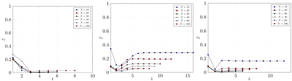
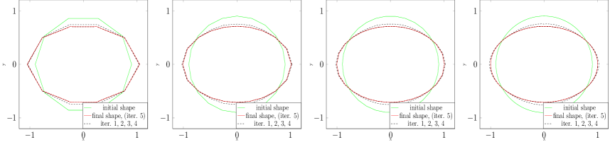
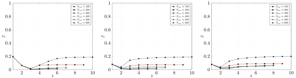
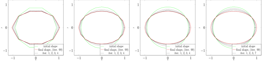
As the convergence rates are only proved for initial shapes sufficiently close to the stationary point, we choose a circle centered at the origin with radius . We select to compare our results with [34]. In the top row of Figure 3 the convergence rates of Newton’s method using different number of control points are shown. In Figure 4 we show several snapshots of the shape progress. We see that all three Hessians yield similar results.
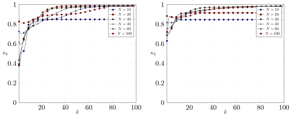
In Figure 6 we study the dependence of the convergence rates on the number of boundary points. Notice that the number of boundary points is not equal to the number of approximate basis functions. In fact in Figure 6 the number of basis functions is kept constant at and the number of boundary points range from to . We see that for all three Hessians the convergence rates improve when we choose more boundary points. In Figure 1 the corresponding function values are displayed. After iteration four the cost function value for all three methods coincide up to the sixth decimal place. We observe that the function value is different for all three methods which means that the three methods compute three different, though very close, stationary points of .

| iteration | domain Hessian | boundary Hessian | approx. Riemannian Hessian |
| 0 | -0.999584093291 | -0.999584093291 | -0.999584093291 |
| 1 | -1.10590500673 | -1.1098402937 | -1.10981595205 |
| 2 | -1.11070220243 | -1.11072033698 | -1.11072034082 |
| 3 | -1.11072032903 | -1.11072049441 | -1.11072048816 |
| 4 | -1.11072032951 | -1.11072049443 | -1.11072048816 |
| 5 | -1.11072032951 | -1.11072049443 | -1.11072048816 |
| 6 | -1.11072032951 | -1.11072049443 | -1.11072048816 |
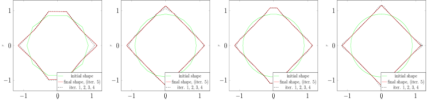
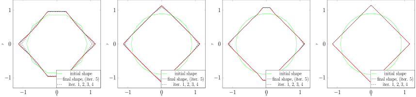
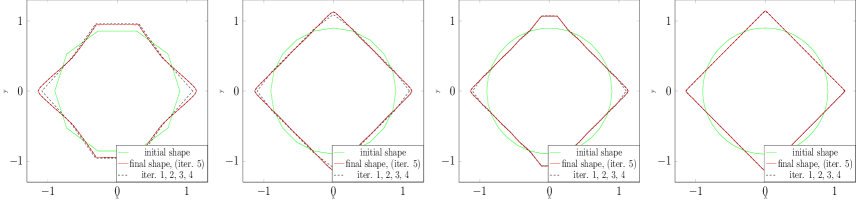
Example 2: square
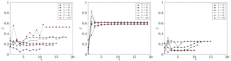
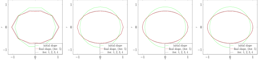
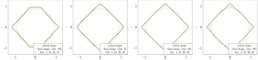
As a second example we take as in (5.1) defined with the function Notice that is weakly differentiable, but it is not continuous differentiable. The minimisation problem has a unique solutions, the domain enclosed by the square . In order to compute the second derivative of we first project the first derivative onto linear finite elements on and take the second derivative of this derivative. The convergence results are shown in the bottom row of Figure 3. The numerical algorithm is terminated if either or if the maximal iteration number of 20 is reached. Some snapshots of the iterations are shown in Figure 5.
5.3 Gradient method
Euclidean metric
We now compare the difference between a gradient and Newton method. For this purpose we choose the Eulcidean metric (see [11]) on the approximate space as inner product. The Euclidean metric is defined by and extend this inner product to . Then the steepest descent direction in this metric given as solution of
| (5.8) |
In each step the domain is updated via with denoting the step size. It is readily seen (cf. [11]) that As an initial shape we take again the domain enclosed by the circle centered at the origin with radius . A constant step size of has been chosen. We terminate the algorithm if either or after maximum of iterations. The results for the square and ellipse are depicted in Figure 8. The difference between the Newton method is both visible from the shape progress and the convergence speed.
Conclusion
In this paper we have examined a Newton method defined via approximate normal functions that can be interpreted as the discretised version of an infinite dimensional Newton method. We introduced two different notions of Hessian, the domain and boundary Hessian. We proved superlinear convergence of a Newton method using the domain Hessian. In general quadratic convergence is lost when the vector fields are only approximated by approximate normal functions. Finally our results are validated by numerical experiments studying the convergence rates dependent on the discretisation.
The thorough numerical investigation using our approximate normal functions also indicates that for large shape deformations the usage of the boundary shape Hessian is favorable. This can be explained by the fact that according to Theorem 2.10 the domain Hessian also contains tangential components which are not entirely eliminated by the approximate normal functions. However when we are close to a stationary domain no significant difference has been observed. Nevertheless for some applications it may make sense to use the domain Hessian and therefore in order to allow for larger shape deformation as well different basis functions that are ”more” normal to the boundary have to be found. Here the difficulty lies in the fact that the domain expression has to be evaluated with vector fields defined on . The search for such novel functions is challenging topic will be part of a future project.
Appendix
Proof of Lemma 4.1.
Proof of Lemma 1.5.
Define , . Then it is readily checked that the recursive formula for holds. Summing over and recalling the telescope sum, we get
| (5.11) |
Then (5.11) together with the fact that are homeomophisms yield
| (5.12) |
Now observe that for all , we have and consequently
| (5.13) |
where in the last step we used for all . Now (5.12) and (5.13) together yield (1.7). ∎
References
- [1] P.-A. Absil, R. Mahony, and R. Sepulchre. Optimization algorithms on matrix manifolds. Princeton University Press, Princeton, NJ, 2008. With a foreword by Paul Van Dooren.
- [2] G. Allaire, E. Cancès, and J.-L. Vié. Second-order shape derivatives along normal trajectories, governed by hamilton-jacobi equations. Structural and Multidisciplinary Optimization, pages 1–22, 2016.
- [3] H. Amann and J. Escher. Analysis. II. Grundstudium Mathematik. [Basic Study of Mathematics]. Birkhäuser Verlag, Basel, 1999.
- [4] D. Bucur and J.-P. Zolésio. Anatomy of the shape Hessian via Lie brackets. Ann. Mat. Pura Appl. (4), 173:127–143, 1997.
- [5] M. Burger. A framework for the construction of level set methods for shape optimization and reconstruction. Interfaces Free Bound., 5(3):301–329, 2003.
- [6] L. Conlon. Differentiable manifolds. Modern Birkhäuser Classics. Birkhäuser Boston, Inc., Boston, MA, second edition, 2008.
- [7] M. C. Delfour and J.-P. Zolésio. Structure of shape derivatives for nonsmooth domains. J. Funct. Anal., 104(1):1–33, 1992.
- [8] M. C. Delfour and J.-P. Zolésio. Shapes and geometries, volume 22 of Advances in Design and Control. Society for Industrial and Applied Mathematics (SIAM), Philadelphia, PA, second edition, 2011. Metrics, analysis, differential calculus, and optimization.
- [9] M. C. Delfour and J.-P. Zolésio. Shapes and geometries, volume 22 of Advances in Design and Control. Society for Industrial and Applied Mathematics (SIAM), Philadelphia, PA, second edition, 2011. Metrics, analysis, differential calculus, and optimization.
- [10] P. Deuflhard. Newton methods for nonlinear problems, volume 35 of Springer Series in Computational Mathematics. Springer, Heidelberg, 2011. Affine invariance and adaptive algorithms, First softcover printing of the 2006 corrected printing.
- [11] M. Eigel and K. Sturm. Reproducing kernel hilbert spaces and variable metric algorithms in PDE-constrained shape optimization. Optimization Methods and Software, 33(2):268–296, may 2017.
- [12] K. Eppler. Second derivatives and sufficient optimality conditions for shape functionals. Control Cybernet., 29(2):485–511, 2000.
- [13] K. Eppler and H. Harbrecht. A regularized Newton method in electrical impedance tomography using shape Hessian information. Control Cybernet., 34(1):203–225, 2005.
- [14] K. Eppler and H. Harbrecht. Second order Lagrange multiplier approximation for constrained shape optimization problems: Mårtensson’s approach for shape problems. In Control and boundary analysis, volume 240 of Lect. Notes Pure Appl. Math., pages 107–118. Chapman & Hall/CRC, Boca Raton, FL, 2005.
- [15] K. Eppler and H. Harbrecht. Second-order shape optimization using wavelet BEM. Optim. Methods Softw., 21(1):135–153, 2006.
- [16] K. Eppler, H. Harbrecht, and R. Schneider. On convergence in elliptic shape optimization. SIAM J. Control Optim., 46(1):61–83 (electronic), 2007.
- [17] G. E. Fasshauer and Q. Ye. Reproducing kernels of Sobolev spaces via a green kernel approach with differential operators and boundary operators. Adv. Comput. Math., 38(4):891–921, 2013.
- [18] M. Frey. Shape Calculus Applied to State-Constrained Elliptic Optimal Control Problems. PhD thesis, University of Bayreuth, Bayreuth, 2012.
- [19] J. Haslinger and R. A. E. Mäkinen. Introduction to shape optimization, volume 7 of Advances in Design and Control. Society for Industrial and Applied Mathematics (SIAM), Philadelphia, PA, 2003. Theory, approximation, and computation.
- [20] A. Henrot and M. Pierre. Variation et optimisation de formes, volume 48 of Mathématiques & Applications (Berlin) [Mathematics & Applications]. Springer, Berlin, 2005. Une analyse géométrique. [A geometric analysis].
- [21] M. Hintermüller and W. Ring. A second order shape optimization approach for image segmentation. SIAM J. Appl. Math., 64(2):442–467 (electronic), 2003/04.
- [22] M. Hintermüller and W. Ring. An inexact Newton-CG-type active contour approach for the minimization of the Mumford-Shah functional. J. Math. Imaging Vision, 20(1-2):19–42, 2004. Special issue on mathematics and image analysis.
- [23] A. Kriegl and P. W. Michor. The convenient setting of global analysis, volume 53 of Mathematical Surveys and Monographs. American Mathematical Society, Providence, RI, 1997.
- [24] J. Lamboley and M. Pierre. Structure of shape derivatives around irregular domains and applications. J. Convex Anal., 14(4):807–822, 2007.
- [25] A. Laurain and K. Sturm. Distributed shape derivative via averaged adjoint method and applications. ESAIM Math. Model. Numer. Anal., 50(4):1241–1267, 2016.
- [26] A. M. Micheletti. Metrica per famiglie di domini limitati e proprietà generiche degli autovalori. Ann. Scuola Norm. Sup. Pisa (3), 26:683–694, 1972.
- [27] P. W. Michor. Manifolds of differentiable mappings, volume 3 of Shiva Mathematics Series. Shiva Publishing Ltd., Nantwich, 1980.
- [28] P. W. Michor and D. Mumford. Riemannian geometries on spaces of plane curves. J. Eur. Math. Soc. (JEMS), 8(1):1–48, 2006.
- [29] M. Nagumo. Über die Lage der Integralkurven gewöhnlicher Differentialgleichungen. Proc. Phys.-Math. Soc. Japan (3), 24:551–559, 1942.
- [30] A. Novruzi and M. Pierre. Structure of shape derivatives. J. Evol. Equ., 2(3):365–382, 2002.
- [31] A. Novruzi and J. R. Roche. Newton’s method in shape optimisation: a three-dimensional case. BIT, 40(1):102–120, 2000.
- [32] W. Ring and B. Wirth. Optimization methods on Riemannian manifolds and their application to shape space. SIAM J. Optim., 22(2):596–627, 2012.
- [33] V. Schulz and M. Siebenborn. Computational comparison of surface metrics for PDE constrained shape optimization. Comput. Methods Appl. Math., 16(3):485–496, 2016.
- [34] V. H. Schulz. A Riemannian view on shape optimization. Found. Comput. Math., 14(3):483–501, 2014.
- [35] Volker H. Schulz, Martin Siebenborn, and Kathrin Welker. Efficient pde constrained shape optimization based on steklov–poincaré-type metrics. SIAM Journal on Optimization, 26(4):2800–2819, 2016.
- [36] J. Simon. Second variations for domain optimization problems. In Control and estimation of distributed parameter systems (Vorau, 1988), volume 91 of Internat. Ser. Numer. Math., pages 361–378. Birkhäuser, Basel, 1989.
- [37] J. Sokołowski and J.-P. Zolésio. Introduction to shape optimization, volume 16 of Springer Series in Computational Mathematics. Springer, Berlin, 1992. Shape sensitivity analysis.
- [38] K. Sturm. On shape optimization with non-linear partial differential equations. PhD thesis, Berlin, Technische Universität Berlin, Diss., 2015.
- [39] K. Sturm. A structure theorem for shape functions defined on submanifolds. Interfaces and Free boundaries, 18(2):523–543, 2016.
- [40] H. Wendland. Piecewise polynomial, positive definite and compactly supported radial functions of minimal degree. Adv. Comput. Math., 4(4):389–396, 1995.
- [41] H. Wendland. On the smoothness of positive definite and radial functions. J. Comput. Appl. Math., 101(1-2):177–188, 1999.
- [42] H. Wendland. Scattered data approximation, volume 17 of Cambridge Monographs on Applied and Computational Mathematics. Cambridge University Press, Cambridge, 2005.
- [43] Z. Mm Wu. Compactly supported positive definite radial functions. Adv. Comput. Math., 4(3):283–292, 1995.
- [44] J.-P. Zolésio. Identification de domains par deformations. PhD thesis, Université de Nice, 1979.