A Factorization Approach to
Inertial Affine Structure from Motion

Abstract

We consider the problem of reconstructing a 3-D scene from a moving camera with high frame rate using the affine projection model. This problem is traditionally known as Affine Structure from Motion (Affine SfM), and can be solved using an elegant low-rank factorization formulation. In this paper, we assume that an accelerometer and gyro are rigidly mounted with the camera, so that synchronized linear acceleration and angular velocity measurements are available together with the image measurements. We extend the standard Affine SfM algorithm to integrate these measurements through the use of image derivatives.

I Introduction

A central problem in geometry in computer vision is Structure from Motion (SfM), which is the problem of reconstructing a 3-D scene from sparse feature points tracked in the images of a moving camera. This problem is known also in the robotics community as Simultaneous Localization and Mapping (SLAM). One of the main differences between the two communities is that in SLAM it is customary to assume the presence of an Inertial Measurement Unit (IMU) that provides measurements of angular velocity and linear acceleration in the camera’s frame. Conversely, in SfM there is a line of work which uses an affine camera model, which is an approximation to the projective model when the depth of the scene is relatively small with respect to the distance between camera and scene. The resulting Affine SfM problem affords a very elegant closed-form solution based on matrix factorization and other linear algebra operations [65]. This solution has not been used in the robotics community, possibly due to the fact that it cannot be immediately extended to use IMU measurements.

We assume that the relative pose between IMU and camera has been calibrated using one of the existing offline [45], online [33, 32, 48, 70, 36] or closed form [19, 53, 52] approaches.

Paper contributions

In this paper we bridge the gap between the two communities by proposing a new Dynamic Affine SfM technique. Our technique is a direct extension of the traditional Affine SfM algorithm, but incorporates synchronized IMU measurements. This is achieved by assuming that the frame rate of the camera is high enough and that we can compute the higher order derivatives of the point trajectories. Remarkably, our formulation leads again to a closed form solution based on matrix factorization and linear algebra operations. To the best of our knowledge, this kind of relation between higher-order derivatives of image trajectories (flow) and IMU measurements, and the low-rank factorization relation between them, have never been exploited before.

II Review of prior work

In the vision community, the Dynamic SfM problem is related to traditional Structure from Motion (SfM), which uses only vision measurements. The standard solution pipeline [28] includes three steps. First, estimate relative poses between pairs of images by using matched features [46, 17, 6] and robust fitting techniques [23, 26]. Second, combine the pairwise estimates either in sequential stages [61, 2, 3, 25, 62], or by using a pose-graph approach [9] (which works only with the poses and not the 3-D structure). Algorithms under the latter category can be divided into local methods [67, 27, 1, 11], which use gradient-based optimization, and global methods [51, 5, 69], which involve a relaxation of the constraints on the rotations together with a low-rank approximation. The fourth and last step of the pipeline is to use Bundle Adjustment (BA) [66, 28, 22], where the motion and structure are jointly estimated by minimizing the reprojection error.

In the robotics community, Dynamic SFM is closely related to other Vision-aided Inertial Navigation (VIN) problems. These include: Visual-Inertial Odometry (VIO), where only the robots’ motion is of interest, and Simultaneous Localization and Mapping (SLAM), where the reconstruction (i.e., map) of the environment is also of interest. Existing approaches to these problems fall between two extremes. On one end of the spectrum we have batch approaches, which are similar to BA with additional terms taking into account the IMU measurements [8, 63]. If obtaining a map of the environment is not important, the optimization problem can be restricted to the poses alone (as in the pose-graph approach in SfM), using the images and IMU measurements to build a so-called factor graph [31, 16, 4]. To speed-up the computations, some of the nodes can be merged using IMU pre-integration [47, 9], and key-frames [39].

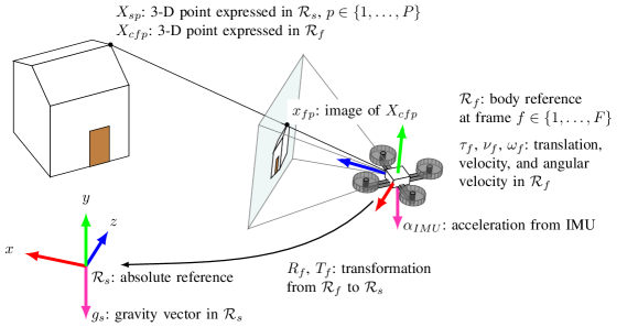
Figure 1: Schematic illustration of the problem and notation.

On the other end of the spectrum we have pure filtering approaches. While some approaches are based on the Unscented Kalman Filter (UKF) [30, 21, 36] or Particle filter [24, 58], the majority are based on the Extended Kalman Filter (EKF). The inertial measurements can be used in either a loosely coupled manner, i.e., in the update step of the filter [40, 56, 10, 33], or in a tightly coupled manner, i.e., in the prediction step of the filter together with a kinematic model [34, 49, 64, 7, 41, 63, 37, 38, 57]. Methods based on the EKF can be combined with an inverse depth parametrization [38, 57, 12, 20] to reduce linearization errors.

Between batch and filtering approaches there are three options. The first is to use incremental solutions to the batch problem [35]. The second option is to use a Sliding Window Filter (SWF) approach, which applies a batch algorithm on a small set of recent measurements. The states that are removed from the window are compressed into a prior term using linearization and marginalization [54, 60, 42, 18, 29], possibly approximating the sparsity of the original problem [14]. The third option is to use a Multistate-Constrained Kalman Filter (MSCKF), which is similar to a sliding window filter, but where the old states are stochastic clones [59] that remain constant and are not updated with the measurements. Comparisons of the two approaches [42, 13] show that the SWF is more accurate and robust, but the MSCKF is more efficient. A hybrid method that switches between the two has appeared in [43], [44].

III Notation and preliminaries

In this section we establish the notation for the following sections. In particular, we define quantities related to a robot (e.g., a quadrotor) equipped with a camera and an inertial measurement unit. We consider its motion as a rigid body, and the relation of this with the IMU measurements and with the geometry of the scene.

Reference frames, transformations and velocities

We first define an inertial spatial frame $\mathcal{R}_{s}$, which corresponds to a fixed “world” reference frame, and a camera reference frame $\mathcal{R}_{f}$, which corresponds to body-fixed reference frame of the robot. For simplicity, we assume that the reference frame of the camera and of the IMU coincide with $\mathcal{R}_{f}$, and that they are both centered at the center of mass of the robot. We denote the world-centered frame as $\mathcal{R}_{s}$, and as $\mathcal{R}_{f}$ the robot-centered frame at some time instant (or “frame”) $f\in\{1,\ldots,F\}$. We also define the pair $(R_{f},T_{f})\in SE(3)$, where $R_{f}$ is a 3-D rotation belonging to the space of rotations $SO(3)$, and $T_{f}\in\real{3}$ is a 3-D translation and $SE(3)$ is the group of rigid body motions [55]. More concretely, given a point with 3-D coordinates $X_{f}\in\real{3}$ in the camera frame, the same point in the spatial frame will have coordinates $X_{s}\in\real{3}$ given by:

$$X_{s}=R_{f}X_{c}+T_{f}.$$ (1)

Note that this equation implies that the $T_{f}$ is equal to the position of the center of mass of the vehicle in $\mathcal{R}_{s}$. Hence, $\dot{T}_{f}$ and $\ddot{T}_{f}$ represent its velocity and acceleration in the same reference frame.

We also define the angular velocity $\omega_{f}\in\real{3}$ with respect to $\mathcal{R}_{f}$ such that

$$\dot{R}_{f}=R_{f}\hat{\omega}_{f},$$ (2)

With this notation, Euler’s equation of motion for the vehicle can be written as [55]:

$$J\dot{\omega}_{f}+\hat{\omega}_{f}J\omega_{f}=\Gamma_{f},$$ (3)

where $J$ is the moment of inertia matrix and $\Gamma_{f}$ is the torque applied to the body, both defined with respect to the local reference frame $\mathcal{R}_{f}$.

Body-fixed quantities

We denote the translation, linear velocity, linear acceleration, rotation and angular velocity of the robot expressed in the reference $\mathcal{R}_{f}$ as $\tau_{f}$, $\nu_{f}$, $\alpha_{f}$, $R_{f}$ and $\omega_{f}$, respectively. Since these are vectors, they are related to the corresponding quantities in the inertial frame $\mathcal{R}_{s}$ by the rotation $R_{f}^{\mathrm{T}}$:

$$\tau_{f} =R_{f}^{\mathrm{T}}T_{f},$$ (4)

$$\nu_{f} =R_{f}^{\mathrm{T}}\dot{T}_{f},$$ (5)

$$\alpha_{f} =R_{f}^{\mathrm{T}}\ddot{T}_{f}.$$ (6)

An ideal body-fixed ideal IMU unit will measure the angular velocity

$$\omega_{IMU}=\omega_{f},$$ (7)

and the acceleration A body-fixed, ideal accelerometer positioned at the center of mass of the object will measure

$$\alpha_{IMU}=R_{f}^{\mathrm{T}}(\ddot{T}_{f}+g_{s})=\alpha_{f}+R_{f}^{\mathrm{T}}g_{s},$$ (8)

where $g_{s}$ is the (downward pointing) gravity vector in the spatial frame $\mathcal{R}_{s}$, around $-9.8e_{z}\mathrm{m}/\mathrm{s}^{2}$, where and $e_{z}=[0\;0\;1]^{\mathrm{T}}$.

Tridimensional structure

We assume that the onboard camera can track the position of $P$ points having coordinates $X_{sp}\in\real{3}$, $p\in\{1,\ldots,P\}$ in $\mathcal{R}_{s}$. For convenience, we assume that $\mathcal{R}_{s}$ is centered at the centroid of this points, that is, $\frac{1}{P}\sum_{p=1}^{P}X_{sp}=0$.

Given the quantities above, we can find expressions for the coordinates of a point in the camera’s coordinate system and its derivatives. However, it is first convenient to find the derivatives of $\tau_{c}$, $\nu_{c}$ and $\omega_{c}$, which can be obtained by combining (4) and (5) with the definition (2), and from Euler’s equation of motion (3).

$$\dot{\tau}_{f} =-\hat{\omega}_{f}\tau_{f}+\nu_{f},$$ (9)

$$\dot{\nu}_{f} =-\hat{\omega}_{f}\nu_{f}+\alpha_{f},$$ (10)

$$\dot{\omega}_{f} =J^{-1}\bigl{(}\Gamma_{f}-\hat{\omega}_{f}J\omega_{f}\bigr{)}.$$ (11)

Then, the coordinate of a point $X_{sp}$ in the reference $\mathcal{R}_{f}$ and its derivatives are given by [55]:

$$X_{cfp}= R_{f}^{\mathrm{T}}X_{sp}-\tau_{f},\qquad$$ (12)

$$\dot{X}_{cfp}= -\hat{\omega}_{f}R_{f}^{\mathrm{T}}X_{sp}+\hat{\omega}_{f}\tau_{f}-\nu_{f},$$ (13)

$$\ddot{X}_{cfp}= \bigl{(}\hat{\omega}_{f}^{2}-\dot{\hat{\omega}}_{f})R_{f}^{\mathrm{T}}X_{sp}-\bigl{(}\hat{\omega}_{f}^{2}-\dot{\hat{\omega}}_{f})\tau_{f}$$

$$+2\hat{\omega}_{f}\nu_{f}-\alpha^{IMU}_{f}-R_{f}^{\mathrm{T}}g_{s},$$ (14)

where $\hat{\cdot}$ denotes the skew-symmetric matrix representation of the cross product [50], and where $\dot{\omega}_{f}$ can be obtained either using Euler’s equation of motion as in (11), by assuming $\dot{\omega}_{f}=0$ (constant velocity model) or by using numerical differentiation of $\omega_{f}$.

Note that $X_{cfp}$ and its derivatives these quantities can be completely determined by the 3-D geometry of the scene in the inertial reference frame, the motion of the camera ($R_{sc}$, $\tau_{c}$, $\nu_{c}$) and the measurements of the IMU ($\alpha_{IMU}$, $\omega_{IMU}$); these all contain some coefficient matrix times the term $R_{f}^{\mathrm{T}}X_{sp}$ plus a vector given by the IMU measurements, the translational motion of the robot and the gravity vector. This structure will lead to the low-rank factorization formulation below.

Image projections

The coordinates in the image of the projection of $X_{sp}$ at frame $f$ is denoted as $x_{fp}$. Assuming that the camera is intrinsically calibrated [50], the image $x_{fp}$ can be related to $X_{cfp}$ with the affine camera model, that is:

$$x_{fp}=\Pi X_{cfp}.$$ (15)

where $\Pi\in\real{2\times 3}$ is a projector that removes the third element of a vector. This model is an approximation of the projective model for when the scene is relatively far from the camera. This model has been used for Affine SfM [65] and Affine Motion Segmentation (see the review article [68] and references within), and it will allow us to introduce the basic principles of our proposed methods.

Using (15), one can show that the images $\{x_{fp}\}$ and their derivatives $\{\dot{x}_{fp}\}$ (flow) and $\{\ddot{x}_{fp}\}$ (double flow) can be written as:

$$x_{fp}= \Pi R_{f}^{\mathrm{T}}X_{sp}-\tau_{f},\qquad$$ (16)

$$\dot{x}_{fp}= -\Pi\hat{\omega}_{f}R_{f}^{\mathrm{T}}X_{sp}+\Pi(\hat{\omega}_{f}\tau_{f}-\nu_{f}),$$ (17)

$$\ddot{x}_{fp}= \Pi\bigl{(}\hat{\omega}_{f}^{2}-\dot{\hat{\omega}}_{f}\bigr{)}R_{f}^{\mathrm{T}}X_{sp}-\Pi\bigl{(}(\hat{\omega}_{f}^{2}-\dot{\hat{\omega}}_{f})\tau_{f}$$ (18)

$$+2\hat{\omega}_{f}\nu_{f}-\alpha^{IMU}_{f}-R_{f}^{\mathrm{T}}g_{s}\bigr{)}.$$ (19)

Formal problem statement

In this section we give the technical details for the proposed Dynamic SfM estimation methods for single agents. The setup and notation used in this section are shown in. We assume that the camera on the robot can track $P$ points for $F$ frames. We assume that the derivatives of the tracked points are available (e.g., through numerical differentiation).

Using the notation introduced in this section, the Dynamic Affine SfM problem is then formulated as finding the motion $\{R_{f},\tau_{f},\nu_{f}\}$, the structure $\{X_{sp}\}$ and the gravity vector $g_{s}$ from the camera measurements $\{x_{fp}\},\{\dot{x}_{fp}\},\{\ddot{x}_{fp}\}$ and the IMU measurements $\{\omega_{f},\alpha^{IMU}_{f}\}$. Figure 1 contains a graphical summary of the problem and of the notation.

IV Dynamic Affine SfM

Factorization formulation

We start our treatment by collecting all the image measurements and their derivatives in a single matrix

$$W=\operatorname{stack}(W^{\prime},\dot{W}^{\prime},\ddot{W}^{\prime})\in\real{6F\times P},$$ (20)

where the matrix $W^{\prime}\in\real{3F\times P}$ is defined by stacking the coordinates $\{x_{fp}\}$ following the frame index $f$ across the rows and the point index $p$ across the columns:

$$W^{\prime}=\begin{bmatrix}x_{11}&\cdots&x_{1P}\\ \vdots&\ddots&\vdots\\ x_{N1}&\cdots&x_{NP}\end{bmatrix}\in\real{2F\times P}.$$ (21)

Notice the common structure in where we have some coefficient matrix times $R_{f}^{\mathrm{T}}$ times $X_{sp}$ plus a vector. Thus, the matrix $W$ admits an affine rank-three decomposition (which can also be written as a rank four decomposition)

$$W=CMS+m=\begin{bmatrix}CM&m\end{bmatrix}\begin{bmatrix}S\\ \mathbf{1}^{\mathrm{T}}\end{bmatrix},$$ (22)

where the motion matrix

$$M=\operatorname{stack}\bigl{(}\{R_{f}^{\mathrm{T}}\}\bigr{)}$$ (23)

contains the rotations, the structure matrix

$$S=\begin{bmatrix}X_{s1}&\cdots&X_{sP}\end{bmatrix}$$ (24)

contains the 3-D points expressed in $\mathcal{R}_{s}$, the coefficient matrix $C$ contains the projector $\Pi$ times the coefficients multiplying the rotations in (14)

$$C=\operatorname{stack}\left(\{\Pi\}_{f=1}^{F},\{-\Pi\hat{\omega}_{f}\}_{f=1}^{F},\{\Pi(\hat{\omega}_{f}^{2}-\dot{\hat{\omega}}_{f})\}_{f=1}^{F}\right),$$ (25)

and the translation vector $m\in\real{2F}$ contains the remaining vector terms

$$m=\operatorname{stack}\bigl{(}\{-\Pi\tau_{f}\}_{f=1}^{F},\{\Pi(\hat{\omega}_{f}\tau_{f}-\nu_{f})\}_{f=1}^{F},\\ \{\Pi((\hat{\omega}_{f}^{2}-\dot{\hat{\omega}}_{f})\tau_{f}+2\hat{\omega}_{f}\nu_{f}-\alpha_{IMU}-R_{f}^{\mathrm{T}}g_{s})\}_{f=1}^{F}\bigr{)}.$$ (26)

In addition to this relation, the quantities $\tau_{f}$, $\nu_{f}$ and $\alpha_{f}^{IMU}$ can be linearly related using derivatives (see (6)). Similarly, $R_{f}$ and $w_{f}$ can be related using the definition of angular velocity. Note that the coefficients $C$ are completely determined by the IMU measurements and the torque inputs.

Optimization formulation

From this, the problem of estimating the motion, the structure, and the gravity direction can then be casted as an optimization problem:

$$\min_{\{R_{f},\tau_{f},\nu_{f}\},g_{s}}\lVert W-(CMS+m)\rVert_{F}^{2}+f_{R}(\{R_{f}\},\{\omega_{f}\})\\ +f_{\tau}(M,\{\tau_{f}\},\{\nu_{f}\})+f_{\nu}(M,\{\nu_{f}\},\{\alpha_{f}^{IMU}\},g_{s}),$$ (27)

where $f_{R}$, $f_{\tau}$ and $f_{\nu}$ are quadratic regularization terms based on approximating the linear derivative constraints between $\tau_{f}$, $\nu_{f}$, $\alpha_{f}^{IMU}$ and between $R_{f}$, $w_{f}$ with finite differences.

In particular, for our implementation we will use,:

$$f_{R} =\sum_{f=1}^{F-1}\lVert R_{f+1}-R_{f}\operatorname{expm}(t_{s}\omega_{f})\rVert_{F}^{2}$$ (28)

$$f_{\tau} =\sum_{f=1}^{F-1}\lVert\frac{1}{t_{s}}\operatorname{conv}(\tau_{k},h_{k},f)-\nu_{f}\rVert_{F}^{2}$$ (29)

$$f_{\nu} =\sum_{f=1}^{F-1}\lVert\frac{1}{t_{s}}\operatorname{conv}(\nu_{k},h_{k},f)-\alpha_{IMU}-R_{f}^{\mathrm{T}}g_{s}\rVert_{F}^{2}.$$ (30)

where with $t_{s}$ is the sampling period of the measurements, $\operatorname{expm}$ is the matrix exponential and $\operatorname{conv}(\tau_{k},h_{k},f)$ gives the sample at time $f$ of the convolution $\tau_{k}\ast h_{k}$ of a signal $\tau_{k}$ with a derivative interpolation filter $h_{k}$. For our implementation we obtain $h_{k}$ from a Savitzky-Golay filter of order one and window size three.

Solution strategy

The optimization problem (27) is non-convex. However, we can find a closed-form solution by exploiting the low-rank nature of the product $MS$ and the linearity of the other terms. This closed-form solution is exact for the noiseless case, and provides an approximated solution to (27) in the noisy case.

1. Factorization. Compute a rank four factorization $W=\tilde{M}\tilde{S}$ using an SVD. With respect to the last term in (22), the factors $\tilde{M}$ and $\tilde{S}$ are related to, respectively $\begin{bmatrix}CM&m\end{bmatrix}$ and $\begin{bmatrix}S\\ \mathbf{1}^{\mathrm{T}}\end{bmatrix}$ by an unknown matrix $K_{\textrm{proj}}\in\real{4\times 4}$. In standard SfM terminology, $\tilde{M}$ and $\tilde{S}$ represent a projective reconstruction.

2. Similarity transformation. Ideally, the last row of $\tilde{S}^{\prime}$ should be $\mathbf{1}^{\mathrm{T}}$. Therefore, we find a vector $k\in\real{4}$ by solving $k^{\mathrm{T}}\tilde{S}^{\prime}=\mathbf{1}^{\mathrm{T}}$ in a least squares sense. We then define the matrix $K_{\textrm{symil}}=\operatorname{stack}(\begin{bmatrix}I&0\end{bmatrix},k^{\mathrm{T}})$, and the matrices $\tilde{M}^{\prime}=\tilde{M}K_{\textrm{symil}}^{-1}$, $\tilde{S}^{\prime}=K_{\textrm{symil}}\tilde{S}$. In standard SfM terminology, $\tilde{M}^{\prime}$ and $\tilde{S}^{\prime}$ represent reconstruction up to a symilarity transformation.

3. Centering. To fix the center of the absolute reference frame $\mathcal{R}_{s}$ to the center of the 3-D structure, we first compute the vector $c=\frac{1}{P}[\tilde{S}^{\prime}]_{1:3,:}$, where $[\tilde{S}^{\prime}]_{1:3,:}$ indicates the matrix composed of the first three rows of $\tilde{S}^{\prime}$. We then define the matrix $K_{\textrm{center}}=\begin{bmatrix}0&-c\\ 0&1\end{bmatrix}$, and the matrices $\tilde{M}^{\prime\prime}=\tilde{M}^{\prime}K_{\textrm{center}}^{-1}$ and $\tilde{S}^{\prime\prime}=K_{\textrm{center}}\tilde{S}^{\prime}$. At this point the forth column of the matrix $\tilde{M}^{\prime\prime}$ contains (in the ideal case) the vector $m$ defined in (22), that is $\hat{m}=[\tilde{M}^{\prime\prime}]_{:,4}$.

4. Recovery of the rotations and structure. We now solve for the rotations $\{R_{f}\}$ by solving a reduced version of (27). In particular, we solve

   $$\min_{M^{\prime\prime}\in\real{3F\times 3}}\lVert[\tilde{M}^{\prime\prime}]_{:,1:3}-CM^{\prime\prime}\rVert_{F}^{2}+\lVert C_{R}M^{\prime\prime}\rVert_{F}^{2},$$ (31)

   where $[\tilde{M}^{\prime\prime}]_{:,1:3}$ indicates the matrix containing the first three columns of $\tilde{M}^{\prime\prime}$, and $C_{R}$ is a block-banded-diagonal matrix with blocks $I$ and $-\operatorname{expm}(t_{s}\omega_{f})^{\mathrm{T}}$ corresponding to the regularization term (28). This is a simple least squares problem which can be easily solved using standard linear algebra algorithms. Ideally, the matrix $M^{\prime\prime}$ is related to the real matrix $M$ by an unknown similarity transformation $K_{\textrm{upg}}\in\real{3\times 3}$. This matrix can be determined (up to an arbitrary rotation) using the standard metric upgrade step from Affine SfM (see [65]). Once $K_{\textrm{upg}}$ has been determined, we define $\hat{M}=M^{\prime\prime}K_{\textrm{upg}}$ and $\hat{S}=K_{\textrm{upg}}^{-1}[\tilde{S}^{\prime\prime}]_{1:3,:}$ to be the estimated motion and structure matrices. The final estimates $\{\hat{R}_{f}\}$ are obtained by projecting each $3\times 3$ block of $\hat{M}$ to $SO(3)$ using an SVD decomposition.

5. Recovery of the translations and linear velocities. We need to extract $\{\tau_{f}\}$ and $\{\omega_{f}\}$ and an estimated gravity direction $\hat{g}_{s}$ from the vector $\hat{m}$. Following (26), we define the matrix

   $$C_{m}=\begin{bmatrix}\vdots&\vdots&\vdots\\ -\Pi&0&0\\ \vdots&\vdots&\vdots\\ \Pi\hat{\omega}_{f}&-\Pi&0\\ \vdots&\vdots&\vdots\\ \Pi((\hat{\omega}_{f}^{2}-\dot{\hat{\omega}}_{f})&2\hat{\omega}_{f}&-R_{f}\\ \vdots&\vdots&\vdots\end{bmatrix}$$ (32)

   and the vector $c_{m}=\operatorname{stack}(\mathbf{0}_{6F},\{\alpha_{f}^{IMU}\})$. Similarly to the definition of $C_{R}$ in (31), we also define the matrices $C_{\tau}$, $C_{\nu}$ corresponding to the regularization terms (29) and (30). We can then solve for the vector $x=\operatorname{stack}(\{\hat{\tau}_{f}\},\{\hat{\nu_{f}\}},\hat{g}_{s})$ by minimizing

   $$\min_{x}\lVert C_{m}x-\hat{m}\rVert_{F}^{2}+\lVert C_{\tau}x\rVert_{F}^{2}+\lVert C_{\nu}x\rVert_{F}^{2},$$ (33)

   which again is a least squares problem that can be solved using standard linear algebra tools.

V Preliminary results

Figure 2 shows a simulation of the result of a preliminary implementation of the Dynamic Affine SfM procedure. We have simulated 5 seconds of a quadrotor following a smooth trajectory while an onboard camera tracks 24 points. The measurements (point coordinates, angular velocity and linear acceleration) are sampled at $30\mathrm{Hz}$ and corrupted with Gaussian noise with variances of the added noise: $3\,\nicefrac{\mathrm{deg}}{\mathrm{s}}$ angular velocity, $0.2\,\nicefrac{\mathrm{m}}{\mathrm{s^{2}}}$ acceleration, $0.5\,\mathrm{\%}$ image points (corresponding to, for instance, $3.2\,\mathrm{px}$ on a $600\times 600\,\mathrm{px}$ image). The reconstruction obtained using our implementation is aligned to the ground-truth using a Procrustes procedure without scaling and compared with an integration of the inertial measurements alone. Figure 3 compares the plot of the ground truth and estimated rotations and translations in absolute coordinates. Three facts should be noted in this simulation: 1. The use of images greatly improves the accuracy with respect to the use of IMU measurements alone. 2. The noise in the estimation mostly appears along the $z$-axis direction of the camera, for which the images do not provide any information. Although ours is a preliminary implementation, the result obtained is extremely close to the ground-truth, except for small errors along the $z$ axis of the camera. These errors are due to the fact that the affine model discards the information along the $z$ axis (the affine model provide little information in this direction, and the reconstruction mostly relies on the noisy accelerometer measurements). 3. Larger noise appears at lower velocities (beginning and end of the trajectory), thus attesting the usefulness of incorporating higher-order derivative information.

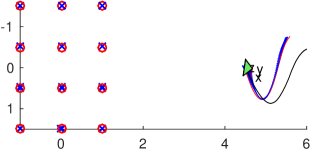
(a) Top view

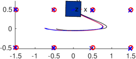
(b) Front view

Figure 2: Simulation results for a preliminary implementation of the Dynamic Affine SfM reconstruction under significantly noisy conditions. Red: ground-truth structure and motion. Blue: reconstructed structure and motion. Black line: motion estimate from integration of IMU measurements alone. Green pyramid: initial reconstructed camera pose. The camera rotates up to $30\,\mathrm{deg}$ and reaches velocities of up to $0.5\,\nicefrac{\mathrm{m}}{\mathrm{s}}$. All axes are in meters.

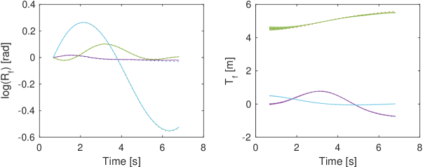
Figure 3: Plots of the ground-truth and estimated trajectories. Left: Absolute rotations in exponential coordinates from the identity, $\log(R_{f})$. Right: absolute translations.

VI Extensions and future work

The approach can be easily extended to the case where multiple (non-overlapping) cameras rigidly mounted to the same IMU. In this case, one can constract multiple matrices $W$ (one for each camera), and performs steps 1–3 of our solution independently. The rotations and translations (steps 4, 5) can then be recovered by solving the linear systems (31) and (33) joinly over all the cameras by adjusting the corresponding coefficient matrices with the relative camera-IMU poses (which are assumed to be known). The Dynamic Affine SfM approach can also be potentially extended to the projective camera model by using the approach of [15]. Let $\Lambda\in\real{F\times P}$ be a matrix containing all the unknown depths of each point in each view, and let $L=\Lambda\otimes\begin{bmatrix}1\\ 1\end{bmatrix}$. Then, one can find a low-rank matrix $\hat{W}$ by minimizing

$$\min_{\hat{W},\Lambda,\dot{\Lambda},\ddot{\Lambda}}\lVert\begin{bmatrix}L\odot W^{\prime}\\ \dot{L}\odot W^{\prime}+L\odot\dot{W}^{\prime}\\ \ddot{L}\odot W^{\prime}+2\dot{L}\odot\dot{W}^{\prime}+L\odot\ddot{W}^{\prime}\end{bmatrix}-\hat{W}\rVert^{2}_{F}\\ +\mu\lVert\hat{W}\rVert_{\ast}+f_{\Lambda}(\Lambda,\dot{\Lambda},\ddot{\Lambda}),$$ (34)

where $\lVert\cdot\rVert_{\ast}$ denotes the nuclear norm (which acts as a low-rank prior for $\hat{W}$), $\mu$ is a scalar weight and $f_{\Lambda}$ relates $\Lambda$ with its derivatives using a derivative interpolation filter. This problem is convex and can be iteratively solved using block coordinate descent (i.e., by minimizing over $\hat{W}$ and the other variables alternatively). The method described in Section IV can then be carried out on the matrix $\hat{W}$ to obtain the reconstruction. Intuitively, (34) estimates the projective depths of each point so that we can reduce the problem to the affine case.

We will implement and evaluate these two extensions in our future work.

References

- [1] K. Aftab, R. Hartley, and J. Trumpf. Generalized weiszfeld algorithms for lq optimization. IEEE Transactions on Pattern Analysis and Machine Intelligence, 37(4):728–745, 2015.
- [2] S. Agarwal, Y. Furukawa, N. Snavely, I. Simon, B. Curless, S. M. Seitz, and R. Szeliski. Building Rome in a day. Communications of the ACM, 54(10):105–112, 2011.
- [3] S. Agarwal, N. Snavely, S. M. Seitz, and R. Szeliski. Bundle adjustment in the large. In IEEE European Conference on Computer Vision, pages 29–42. Springer, 2010.
- [4] M. Agrawal. A lie algebraic approach for consistent pose registration for general euclidean motion. In IEEE International Conference on Intelligent Robots and Systems, pages 1891–1897, 2006.
- [5] M. Arie-Nachimson, S. Kovalsky, I. Kemelmacher-Shlizerman, A. Singer, and R. Basri. Global motion estimation from point matches. In International Conference on 3D Imaging, Modeling, Processing, Visualization and Transmission, pages 81–88, 2012.
- [6] H. Bay, A. Ess, T. Tuytelaars, and L. V. Gool. Speeded-up robust features (SURF). Computer Vision and Image Understanding, 110(3):346–359, 2008.
- [7] R. Brockers, S. Susca, D. Zhu, and L. Matthies. Fully self-contained vision-aided navigation and landing of a micro air vehicle independent from external sensor inputs. In SPIE Defense, Security, and Sensing, page 83870Q. International Society for Optics and Photonics, 2012.
- [8] M. Bryson, M. Johnson-Roberson, and S. Sukkarieh. Airborne smoothing and mapping using vision and inertial sensors. In IEEE International Conference on Robotics and Automation, pages 2037–2042, 2009.
- [9] L. Carlone, R. Tron, K. Daniilidis, and F. Dellaert. Initialization techniques for 3D SLAM: a survey on rotation estimation and its use in pose graph optimization. In IEEE International Conference on Robotics and Automation, 2015.
- [10] L. Chai, W. A. Hoff, and T. Vincent. Three-dimensional motion and structure estimation using inertial sensors and computer vision for augmented reality. Presence: Teleoperators and Virtual Environments, 11(5):474–492, 2002.
- [11] A. Chatterjee and V. M. Govindu. Efficient and robust large-scale rotation averaging. In IEEE International Conference on Computer Vision, pages 521–528, 2013.
- [12] J. Civera, A. J. Davison, and J. M. M. Montiel. Unified inverse depth parametrization for monocular slam. In Robotics: Science and Systems, 2006.
- [13] L. E. Clement, V. Peretroukhin, J. Lambert, and J. Kelly. The battle for filter supremacy: A comparative study of the multi-state constraint Kalman Filter and the Sliding Window Filter. In IEEE Conference on Computer and Robot Vision, pages 23–30, 2015.
- [14] E. D. N. D, K. J. Wu, and S. Roumeliotis. C-KLAM: Constrained keyframe-based localization and mapping. In IEEE International Conference on Robotics and Automation, pages 3638–3643, 2014.
- [15] Y. Dai, H. Li, and M. He. Projective multiview structure and motion from element-wise factorization. IEEE Transactions on Pattern Analysis and Machine Intelligence, 35(9):2238–2251, 2013.
- [16] F. Dellaert and et al. Georgia tech smoothing and mapping (GTSAM). http://tinyurl.com/gtsam.
- [17] J. Dong and S. Soatto. Domain-size pooling in local descriptors: DSP-SIFT. In IEEE Conference on Computer Vision and Pattern Recognition, pages 5097–5106, 2015.
- [18] T.-C. Dong-Si and A. I. Mourikis. Motion tracking with fixed-lag smoothing: Algorithm and consistency analysis. In IEEE International Conference on Robotics and Automation, pages 5655–5662, 2011.
- [19] T.-C. Dong-Si and A. I. Mourikis. Estimator initialization in vision-aided inertial navigation with unknown camera-imu calibration. In IEEE International Conference on Intelligent Robots and Systems, pages 1064–1071, 2012.
- [20] E. Eade and T. Drummond. Scalable monocular SLAM. In IEEE Conference on Computer Vision and Pattern Recognition, volume 1, pages 469–476, 2006.
- [21] S. Ebcin and M. Veth. Tightly-coupled image-aided inertial navigation using the unscented kalman filter. In International Technical Meeting of the Satellite Division of The Institute of Navigation (GNSS), pages 1851–1860, 2001.
- [22] E. C. Engels, H. Stewénius, and D. Nistér. Bundle adjustment rules. In Photogrammetric Computer Vision, volume 2, pages 124–131, 2006.
- [23] M. A. Fischler and R. C. Bolles. Random sample consensus: a paradigm for model fitting with applications to image analysis and automated cartography. Communications of the ACM, 24(6):381–395, 1981.
- [24] D. Fox, W. Burgard, and S. Thrun. Markov localization for mobile robots in dynamic environments. Journal of Artificial Intelligence Research, pages 391–427, 1999.
- [25] J.-M. Frahm, P. Fite-Georgel, D. Gallup, T. Johnson, R. Raguram, C. Wu, Y.-H. Jen, E. Dunn, B. Clipp, S. Lazebnik, and M. Pollefeys. Building Rome on a cloudless day. In IEEE European Conference on Computer Vision, pages 368–381. Springer, 2010.
- [26] R. Hartley and H. Li. An efficient hidden variable approach to minimal-case camera motion estimation. IEEE Transactions on Pattern Analysis and Machine Intelligence, 2012.
- [27] R. Hartley, J. Trumpf, Y. Dai, and H. Li. Rotation averaging. International Journal of Computer Vision, 103(3):267–305, 2013.
- [28] R. I. Hartley and A. Zisserman. Multiple View Geometry in Computer Vision. Cambridge University Press, second edition, 2004.
- [29] G. P. Huang, A. I. Mourikis, and S. Roumeliotis. An observability-constrained sliding window filter for slam. In IEEE International Conference on Intelligent Robots and Systems, pages 65–72, 2011.
- [30] A. Huster, E. W. Frew, and S. M. Rock. Relative position estimation for auvs by fusing bearing and inertial rate sensor measurements. In MTS/IEEE OCEANS, volume 3, pages 1863–1870, 2002.
- [31] V. Indelman and F. Dellaert. Incremental light bundle adjustment: Probabilistic analysis and application to robotic navigation. In New Development in Robot Vision, pages 111–136. Springer, 2015.
- [32] E. Jones, A. Vedaldi, and S. Soatto. Inertial structure from motion with autocalibration. In Workshop on Dynamical Vision, 2007.
- [33] E. S. Jones and S. Soatto. Visual-inertial navigation, mapping and localization: A scalable real-time causal approach. The International Journal of Robotics Research, 30(4):407–430, 2011.
- [34] S.-H. Jung and C. J. Taylor. Camera trajectory estimation using inertial sensor measurements and structure from motion results. In IEEE Conference on Computer Vision and Pattern Recognition, volume 2, pages –732. IEEE, 2001.
- [35] M. Kaess, H. Johannsson, R. Roberts, V. Ila, J. J. Leonard, and F. Dellaert. iSAM2: Incremental smoothing and mapping using the bayes tree. The International Journal of Robotics Research, pages 1–20, 2011.
- [36] J. Kelly and G. S. Sukhatme. Visual-inertial sensor fusion: Localization, mapping and sensor-to-sensor self-calibration. The International Journal of Robotics Research, 30(1):56–79, 2011.
- [37] J.-H. Kim and S. Sukkarieh. Airborne simultaneous localisation and map building. In IEEE International Conference on Robotics and Automation, volume 1, pages 406–411, 2003.
- [38] M. Kleinert and S. Schleith. Inertial aided monocular SLAM for GPS-denied navigation. In IEEE Conference on Multisensor Fusion and Integration for Intelligent Systems, pages 20–25, 2010.
- [39] K. Konolige and M. Agrawal. FrameSLAM: From bundle adjustment to real-time visual mapping. IEEE Transactions on Robotics and Automation, 24(5):1066–1077, 2008.
- [40] K. Konolige, M. Agrawal, and J. Sola. Large-scale visual odometry for rough terrain. In Robotics Research, pages 201–212. Springer, 2011.
- [41] D. G. Kottas and S. I. Roumeliotis. Exploiting urban scenes for vision-aided inertial navigation. In Robotics: Science and Systems, 2013.
- [42] S. Leutenegger, S. Lynen, M. Bosse, R. Siegwart, and P. Furgale. Keyframe-based visual-inertial odometry using nonlinear optimization. The International Journal of Robotics Research, 34(3):314–334, 2015.
- [43] M. Li and A. Mourikis. Vision-aided inertial navigation for resource-constrained systems. In IEEE International Conference on Intelligent Robots and Systems, pages 1057–1063, 2012.
- [44] M. Li and A. I. Mourikis. Optimization-based estimator design for vision-aided inertial navigation. In Robotics: Science and Systems, pages 241–248, 2013.
- [45] J. Lobo and J. Dias. Relative pose calibration between visual and inertial sensors. The International Journal of Robotics Research, 26(6):561–575, 2007.
- [46] D. G. Lowe. Distinctive image features from scale-invariant keypoints. International Journal of Computer Vision, 60(2):91–110, 2004.
- [47] T. Lupton and S. Sukkarieh. Visual-inertial-aided navigation for high-dynamic motion in built environments without initial conditions. IEEE Transactions on Robotics and Automation, 28(1):61–76, 2012.
- [48] S. Lynen, M. W. Achtelik, S. Weiss, M. Chli, and R. Siegwart. A robust and modular multi-sensor fusion approach applied to MAV navigation. In IEEE International Conference on Intelligent Robots and Systems, pages 3923–3929, 2013.
- [49] J. Ma, S. Susca, M. Bajracharya, L. Matthies, M. Malchano, and D. Wooden. Robust multi-sensor, day/night 6-DOF pose estimation for a dynamic legged vehicle in GPS-denied environments. In IEEE International Conference on Robotics and Automation, pages 619–626, 2012.
- [50] Y. Ma. An invitation to 3-D vision: from images to geometric models. Springer, 2004.
- [51] D. Martinec and T. Pajdla. Robust rotation and translation estimation in multiview reconstruction. In IEEE Conference on Computer Vision and Pattern Recognition, pages 1–8, 2007.
- [52] A. Martinelli. Vision and imu data fusion: Closed-form solutions for attitude, speed, absolute scale, and bias determination. IEEE Transactions on Robotics and Automation, 28(1):44–60, 2012.
- [53] A. Martinelli. Observabilty properties and deterministic algorithms in visual-inertial structure from motion. Foundations and Trends in Robotics, pages 1–75, 2013.
- [54] C. Mei, G. Sibley, M. Cummins, P. Newman, and I. Reid. RSLAM: A system for large-scale mapping in constant-time using stereo. International Journal of Computer Vision, 94(2):198–214, 2011.
- [55] R. M. Murray, Z. Li, and S. S. Sastry. A Mathematical Introduction to Robotic Manipulation. CRC Press, 1994.
- [56] T. Oskiper, Z. Zhu, S. Samarasekera, and R. Kumar. Visual odometry system using multiple stereo cameras and inertial measurement unit. In IEEE Conference on Computer Vision and Pattern Recognition, pages 1–8, 2007.
- [57] P. Piniés, T. Lupton, S. Sukkarieh, and J. D. Tardós. Inertial aiding of inverse depth slam using a monocular camera. In IEEE International Conference on Robotics and Automation, pages 2797–2802, 2007.
- [58] M. Pupilli and A. Calway. Real-time camera tracking using a particle filter. In British Machine Vision Conference, 2005.
- [59] S. Roumeliotis, A. E. Johnson, and J. F. Montgomery. Augmenting inertial navigation with image-based motion estimation. In IEEE International Conference on Robotics and Automation, volume 4, pages 4326–4333. IEEE, 2002.
- [60] G. Sibley, L. Matthies, and G. Sukhatme. Sliding window filter with application to planetary landing. Journal of Field Robotics, 27(5):587–608, 2010.
- [61] N. Snavely, S. M. Seitz, and R. Szeliski. Photo tourism: exploring photo collections in 3D. In ACM Transactions on Graphics, volume 25, pages 835–846, 2006.
- [62] N. Snavely, S. M. Seitz, and R. Szeliski. Skeletal graphs for efficient structure from motion. In IEEE Conference on Computer Vision and Pattern Recognition, volume 1, page 2, 2008.
- [63] D. Strelow and S. Singh. Motion estimation from image and inertial measurements. The International Journal of Robotics Research, 23(12):1157–1195, 2004.
- [64] J.-P. Tardif, M. George, M. Laverne, A. Kelly, and A. Stentz. A new approach to vision-aided inertial navigation. In IEEE International Conference on Intelligent Robots and Systems, pages 4161–4168, 2010.
- [65] C. Tomasi and T. Kanade. Shape and motion from image streams under orthography: a factorization method. International Journal of Computer Vision, 9(2):137–154, 1992.
- [66] B. Triggs, P. F. McLauchlan, R. I. Hartley, and A. W. Fitzgibbon. Bundle adjustment – a modern synthesis. In Vision algorithms: theory and practice, pages 298–372. Springer, 2000.
- [67] R. Tron and R. Vidal. Distributed 3-D localization of camera sensor networks from 2-D image measurements. IEEE Transactions on Automatic Control, 2014.
- [68] R. Vidal. Subspace clustering. IEEE Signal Processing Magazine, 2(28):52–68, 2011.
- [69] L. Wang and A. Singer. Exact and stable recovery of rotations for robust synchronization. Information and Inference, 2(2):145–193, 2013.
- [70] S. Weiss, M. W. Achtelik, S. Lynen, M. Chli, and R. Siegwart. Real-time onboard visual-inertial state estimation and self-calibration of MAVs in unknown environments. In IEEE International Conference on Robotics and Automation, pages 957–964, 2012.