The 2-degree Field Lensing Survey: design and clustering measurements

Abstract

We present the 2-degree Field Lensing Survey (2dFLenS), a new galaxy redshift survey performed at the Anglo-Australian Telescope. 2dFLenS is the first wide-area spectroscopic survey specifically targeting the area mapped by deep-imaging gravitational lensing fields, in this case the Kilo-Degree Survey. 2dFLenS obtained $70{,}079$ redshifts in the range $z<0.9$ over an area of $731$ deg², and is designed to extend the datasets available for testing gravitational physics and promote the development of relevant algorithms for joint imaging and spectroscopic analysis. The redshift sample consists first of $40{,}531$ Luminous Red Galaxies (LRGs), which enable analyses of galaxy-galaxy lensing, redshift-space distortion, and the overlapping source redshift distribution by cross-correlation. An additional $28{,}269$ redshifts form a magnitude-limited ($r<19.5$) nearly-complete sub-sample, allowing direct source classification and photometric-redshift calibration. In this paper, we describe the motivation, target selection, spectroscopic observations, and clustering analysis of 2dFLenS. We use power spectrum multipole measurements to fit the redshift-space distortion parameter of the LRG sample in two redshift ranges $0.15<z<0.43$ and $0.43<z<0.7$ as $\beta=0.49\pm 0.15$ and $\beta=0.26\pm 0.09$, respectively. These values are consistent with those obtained from LRGs in the Baryon Oscillation Spectroscopic Survey. 2dFLenS data products will be released via our website http://2dflens.swin.edu.au.

1 Introduction

A wide set of cosmological observations suggests that the dynamics of the Universe are currently dominated by some form of ‘dark energy’, which in standard Friedmann-Robertson-Walker (FRW) models is propelling an acceleration in late-time cosmic expansion. However, the physical nature of dark energy is not yet understood, and its effects are subject to intense observational scrutiny.

Efforts in this area to date have focused on mapping out the cosmic expansion history using baryon acoustic oscillations (BAOs) as a standard ruler (e.g. Beutler et al. 2011, Blake et al. 2011b, Anderson et al. 2014, Kazin et al. 2014, Delubac et al. 2015, Aubourg et al. 2015, Alam et al. 2016) and Type Ia supernovae as standard candles (e.g. Conley et al. 2011, Suzuki et al. 2012, Betoule et al. 2014). These probes have yielded important constraints on the ‘homogeneous expanding Universe’, including $\sim 1\%$ distance measurements and a $\sim 5\%$ determination of the value of the equation-of-state of dark energy, $w$. However, measurements of the laws of gravity that describe the ‘clumpy Universe’ are currently less advanced, and only a combination of complementary observations of expansion and gravitational growth will discriminate between the different possible physical manifestations of dark energy. Efforts have focused on establishing whether the laws of General Relativity (GR), well-tested on solar-system scales, are a good description of gravity on cosmological scales 14 orders of magnitude larger.

There are two particularly important observable signatures of gravitational physics that can be used for this purpose, and these two methods gain considerable leverage when combined. The first observable is the peculiar motions of galaxies as they fall toward overdense regions as non-relativistic test particles. These motions produce correlated Doppler shifts in galaxy redshifts that create an overall clustering anisotropy as a function of the angle to the line-of-sight, known as redshift-space distortion (RSD). This pattern has been measured by a number of galaxy redshift surveys (e.g. Blake et al. 2011a, Beutler et al. 2012, de la Torre et al. 2013, Samushia et al. 2014, Beutler et al. 2014, Marin et al. 2016, Alam et al. 2016) and has permitted the growth rate of cosmic structure to be measured with $\sim 10\%$ accuracy at some epochs. The second gravitational probe is the patterns of weak lensing imprinted by the deflections of light rays from distant galaxies as they travel through the intervening large-scale structure as relativistic test particles. This signal may be measured using correlations in the apparent shapes of background galaxies in deep imaging surveys (e.g. Heymans et al. 2012, Huff et al. 2014, Kuijken et al. 2015, Becker et al. 2016, Hildebrandt et al. 2016b). Whilst the cosmological parameter constraints possible from gravitational lensing statistics are still improving, the measurement offers several key advantages such as its insensitivity to galaxy bias.

Velocities and lensing are complementary because only their combination allows general deviations to the Einstein field equations to be constrained (Zhang et al. 2007, Song et al. 2011). Modern theories of gravity may be classified by the manner in which they warp or perturb the spacetime metric (and the way this warping is generated by matter). In general two types of perturbations are possible: spacelike and timelike. In GR these perturbations are equal and opposite, but in ‘modified gravity’ scenarios a difference is predicted. Examples of such frameworks include generalizing the ‘action’ of GR as a function of the Ricci curvature, such as in $f(R)$ gravity models (Sotiriou & Faraoni 2010), or embedding ordinary 3+1 dimensional space into a higher-dimensional manifold such as ‘Cascading gravity’ (de Rham et al. 2008) or ‘Galileon gravity’ (Chow & Khoury 2009). These scenarios make different observable predictions.

Joint cosmological fits to weak gravitational lensing and galaxy redshift-space distortion statistics can be performed using datasets without sky overlap (e.g. Simpson et al. 2013). However, the availablity of overlapping imaging and spectroscopic surveys yields several scientific benefits. First, since the same density fluctuations source both the lensing and galaxy velocity signals, the partially-shared sample variance reduces the uncertainty in the gravity fits (McDonald & Seljak 2009), and the addition of the shape-density correlation statistics (‘galaxy-galaxy lensing’) enables new measurements to be constructed such as the ‘gravitational slip’ (Zhang et al. 2007). A series of authors (Gaztanaga et al. 2012; Cai & Bernstein 2012; de Putter, Dore & Das 2014; Kirk et al. 2015; Eriksen & Gaztanaga 2015) have predicted statistical improvements resulting from overlapping surveys, although the degree of this improvement depends on assumptions and survey configuration (Font-Ribera et al. 2014).

Perhaps more importantly, the actual benefit of overlapping surveys exceeds statistical forecasts because weak lensing measurements are limited by a number of sources of systematic error which may be mitigated using same-sky spectroscopic-redshift observations. One of the most significant systematic errors is the calibration of the source photometric redshifts which are required for cosmic shear tomography (Ma, Hu & Huterer 2006). Overlapping spectroscopic surveys are a powerful means of performing this calibration (Newman et al. 2015), using approaches including both observation of complete spectroscopic sub-samples and analysis of cross-correlation statistics (McQuinn & White 2013, de Putter, Dore & Das 2014). Conversely, the gravitational lensing imprint allows independent calibration of the galaxy bias parameters that are a key systematic limitation to redshift-space distortion analysis (e.g. Buddendiek et al. 2016). Finally, overlapping imaging and spectroscopy enables a wide range of other science including studies of galaxy clusters, strong lensing systems and galaxy evolution.

The first wide-area overlapping spectroscopic and cosmic shear surveys only recently became available and currently span a shared area of $\sim 500$ deg², consisting of an overlap between two lensing imaging surveys – the Canada-France-Hawaii Telescope Legacy Survey (CFHTLS; Gwyn 2012, Heymans et al. 2012) and the 2nd Red Sequence Cluster Survey (RCS2; Gilbank et al. 2011, Hildebrandt et al. 2016a) – and two spectroscopic redshift surveys – the WiggleZ Dark Energy Survey (Drinkwater et al. 2010) and the Baryon Oscillation Spectroscopic Survey (BOSS; Dawson et al. 2013). This overlap has permitted a number of studies including a new consistency test of GR via a measurement of gravitational slip at $z=0.6$ (Blake et al. 2016), joint constraints on halo occupation distribution and cosmological parameters (More et al. 2015), tests of imaging photometric redshift performance via cross-correlation (Choi et al. 2016) and new measurements of small-scale galaxy bias parameters (Buddendiek et al. 2016).

Wide-area overlap between spectroscopic and imaging surveys requires significant further extension to realize its full scientific potential. Two of the deep imaging surveys currently being performed to measure gravitational lensing – the 1500 deg² Kilo-Degree Survey (KiDS; Kuijken et al. 2015) at the European Southern Observatory VLT Survey Telescope (VST), and the 5000 deg² Dark Energy Survey (DES; Becker et al. 2016) at the Blanco Telescope – are located largely in the southern hemisphere, whereas the largest existing wide-area spectroscopic surveys have been carried out by the Sloan Telescope in the northern hemisphere. With this in mind, we have created the 2-degree Field Lensing Survey (2dFLenS), a new southern-hemisphere spectroscopic redshift survey using the Anglo-Australian Telescope (AAT). The 2dF-AAOmega multi-fibre spectroscopic system at the AAT has conducted a series of such projects including the 2-degree Field Galaxy Redshift Survey (2dFGRS; Colless et al. 2001), the WiggleZ Dark Energy Survey (Drinkwater et al. 2010), the Galaxy And Mass Assembly survey (GAMA; Driver et al. 2011), and OzDES (Yuan et al. 2015).

This paper describes the design, performance and initial clustering analysis of 2dFLenS. Key initial scientific analyses, some in conjunction with KiDS, are presented by five associate papers (Joudaki et al. 2016b, Johnson et al. 2016, Amon et al. 2016, Wolf et al. 2016, Janssens et al. 2016). Section 2 motivates the survey design: the choice of fields and targets. Section 3 describes the process of selecting targets from input photometric imaging catalogues, and Section 4 discusses the spectroscopic observing campaign including AAT data reduction and galaxy redshift determination. Section 5 describes the calculation of the selection function of the spectroscopic observations, which forms the basis of the ensuing galaxy clustering measurements. Section 6 outlines the construction of the survey mock catalogues which are used to estimate the covariance matrix of the clustering statistics, whose measurement is discussed in Section 7. We summarize in Section 8.

2 Survey design

2.1 Choice of fields

The purpose of 2dFLenS is to extend the coverage of spectroscopic-redshift observations that overlap with deep optical imaging surveys performed to measure weak gravitational lensing. The principal focus of our new spectroscopic coverage is the area being imaged by the Kilo-Degree Survey (KiDS; de Jong et al. 2015, Kuijken et al. 2015), a new lensing dataset in the southern sky. The KiDS footprint is planned to encompass 1500 deg², divided into two approximately equal areas around the Southern Galactic Cap (SGC) and Northern Galactic Cap (NGC). Approximately 500 deg² of the KiDS NGC survey region is already covered by deep spectroscopic data provided by the Baryon Oscillation Spectroscopic Survey (BOSS; Dawson et al. 2013). The remaining KiDS area lacks deep, wide-area spectroscopic coverage, although two shallower redshift surveys have performed overlapping observations: the Galaxy And Mass Assembly survey (GAMA; Driver et al. 2011) and the 2-degree Field Galaxy Redshift Survey (2dFGRS; Colless et al. 2001). However, neither of these existing datasets has the depth nor coverage to address our scientific aims.

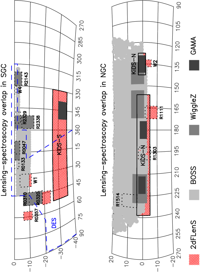
In addition to the KiDS region, 2dFLenS also conducted observations in sky areas covered by two other deep lensing imaging surveys: the Canada France Hawaii Telescope Legacy Survey (CFHTLS; Gwyn 2012, Heymans et al. 2012) and the 2nd Red Sequence Cluster Survey (RCS2; Gilbank et al. 2011, Hildebrandt et al. 2016a). In particular, we targeted regions of those surveys which possessed either no or partial deep spectroscopic follow-up: CFHTLS regions W1 and W2, and RCS2 regions 0320, 0357 and 1111. The right ascension and declination boundaries of all these fields are listed in Table 1.

Figure 1: Locations of current spectroscopic and imaging surveys in the Southern Galactic Cap (SGC) and Northern Galactic Cap (NGC). Deep spectroscopic surveys (BOSS, WiggleZ and GAMA) are indicated as grey shaded regions. Deep imaging surveys (CFHTLS, RCS2 and KiDS) are displayed as outlined rectangles, labelled by field names. The approximate DES footprint is located inside the dashed blue line. The originally-planned 2dFLenS spectroscopic coverage is displayed using cross-hatched red shading and spans almost 1000 deg².

Table 1: Right Ascension and Declination boundaries in degrees of regions targeted for observation by 2dFLenS. The top and bottom halves of the table list SGC and NGC regions, respectively.

Region	min R.A.	max R.A.	min Dec.	max Dec.
KiDS-S	330.0	52.5	-36.0	-26.0
RCS 0320	44.0	53.2	-24.1	-18.5
RCS 0357	56.3	62.2	-11.7	-6.0
CFHTLS W1	30.1	38.9	-11.3	-3.7
KiDS-N (1)	127.5	142.5	-2.0	3.0
KiDS-N (2)	156.0	238.5	-5.0	4.0
RCS 1111	163.7	172.3	-10.1	-1.7
CFHTLS W2	132.0	136.9	-5.8	-0.9

Figure 1 illustrates the location of these regions in more detail. The cross-hatched red shaded area indicates the fields originally planned to be targeted for observation by 2dFLenS, extending existing coverage by BOSS. This area comprised a total of 985 deg² (731 and 254 deg² in the SGC and NGC, respectively). Our observations also overlap with the footprint of the Dark Energy Survey (DES). The final status of our spectroscopic campaign is illustrated in Figure 2 and discussed in Section 4.5.

We tiled the 2dFLenS observation regions with 2-degree diameter circular pointings of the 2dF+AAOmega spectroscopic system at the Anglo-Australian Telescope (AAT), using a hexagonal pointing grid with fixed field centres. Usage of a fixed pointing grid, rather than an adaptive, overlapping pointing grid, simplifies the determination of the angular completeness of the observations via a ratio of successful redshifts to intended targets computed in unique sectors. In total we defined 324 AAT pointing centres, 245 in the SGC and 79 in the NGC, which were suitable for observation. The distribution of these field centres is displayed in Figure 2. We excluded a small fraction of intended field centres which lacked appropriate input imaging data as discussed in Section 3.

Figure 2: The final coverage of 2dFLenS observations within the deep imaging survey regions outlined by the red rectangles. The dark points display the locations of successful 2dFLenS galaxy redshifts, with BOSS galaxy redshifts indicated by the blue points. The originally-planned 2dFLenS AAT pointings are displayed as the black circles, observations suffering low completeness at the end of the survey are indicated by orange circles, and unobserved pointings are highlighted in magenta.

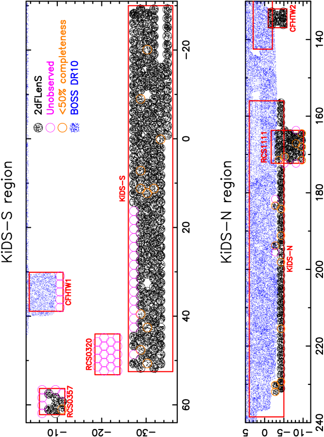
The 2dFLenS project applied for competitive time allocation at the AAT in March 2014 and was allocated a total of 53 nights spread across the 14B, 15A and 15B semesters, the majority of which occurred in ‘grey time’ with regard to moon phase.

2.2 Choice of targets

The set of galaxies targeted for spectroscopic observation by 2dFLenS was selected to enable two principal scientific goals:

• Measurement of the gravitational lensing signal imprinted by the spectroscopic targets in the apparent shapes of background sources (‘galaxy-galaxy lensing’), and the comparison of this lensing signal with the amplitude of galaxy peculiar velocities driven by the same density fluctuations, across a wide redshift range.

• Determination of the source redshift distribution in the overlapping imaging survey, using both direct photometric-redshift calibration (enabled by spectroscopy of a complete sub-sample) and cross-correlation techniques (using the clustering between the imaging sources and the spectroscopic sample in narrow redshift slices).

The optimal choice of targets for the first goal, whose correlation with background source shapes will maximize the resulting galaxy-galaxy lensing signal, is Luminous Red Galaxies (LRGs), which preferentially trace dense areas of the Universe and hence imprint the strongest gravitational lensing signal. Bright LRGs in the redshift range $z<1$ can be readily selected using well-understood colour and magnitude cuts developed by previous observational projects such as the Sloan Digital Sky Survey (SDSS, Eisenstein et al. 2001), the 2dF-SDSS LRG And Quasar survey (2SLAQ, Cannon et al. 2006), the Baryon Oscillation Spectroscopic Survey (BOSS, Dawson et al. 2013) and the Extended Baryon Oscillation Spectroscopic Survey (eBOSS, Dawson et al. 2016). We utilized these colour cuts, which are inspired by the evolution with redshift of an early-type galaxy template, in particular the 4000Å spectral break, through the optical filter system. The majority of our survey area overlaps with KiDS, which has a weighted mean redshift of $\sim 0.7$ (Kuijken et al. 2015), where the weights reflect the accuracy of the weak lensing shape measurement for each object. We therefore prioritized spectroscopic targets with $z<0.7$ to maximise the number of lenses that are in front of our source galaxies.

A disadvantage of targetting an LRG lens sample for our test of gravitational physics is that its high galaxy bias factor, $b\approx 2$, results in a low redshift-space distortion (RSD) signal, whose amplitude is determined by the parameter $\beta=f/b$ where $f$ is the growth rate of cosmic structure. The higher galaxy-galaxy lensing signal, however, compensates for the lower RSD signal, rendering LRGs the optimal choice of target for this scientific goal.

Turning now to the second goal: determination of the source redshift distribution by cross-correlation mandates a spectroscopic sample overlapping the imaging data across the widest possible redshift range, but (unlike direct photometric-redshift calibration) is agnostic regarding the spectroscopic sample’s galaxy type, which is a matter of observational convenience. Given that our available target-selection imaging is insufficiently deep for efficient identification of high-redshift emission-line galaxies, we utilized LRGs for this purpose as well. The practical limitations of our target-selection imaging, together with the integration time available for our observations, restricted the accessible redshift range to $z<0.9$.

Finally, photometric-redshift determination by direct calibration requires the construction of complete spectroscopic-redshift datasets spanning volumes sufficiently large to minimize the impact of sample variance on this calibration (Cunha et al. 2012). We therefore selected a random sub-sample of galaxies to facilitate this set of investigations, within a magnitude range defined by a faint limit ($r\approx 19.5$) ensuring highly complete redshift determination in all observing conditions, and a bright limit ($r\approx 17$) minimizing overlap with current and future wide-area complete spectroscopic samples such as 2dFGRS, SDSS and the Taipan Galaxy Survey. Given that the clustering of this magnitude-limited sample does not need to be measured, it serves as an ideal set of ‘filler’ targets which can be prioritized below the LRGs scheduled for observation in each AAT pointing, ensuring that all spectroscopic fibres are allocated.

In addition to our main target classes, we also included a set of sparsely-distributed ‘spare fibre’ targets within the 2dFLenS observations. These samples are described in Section 3.4.

3 Target selection

3.1 Imaging catalogues for target selection

2dFLenS targets are selected using a variety of photometric catalogues, depending on the sky area of observation. The majority of 2dFLenS pointings are located within the KiDS survey footprint. However, KiDS imaging observations were still ongoing when 2dFLenS commenced, and therefore it was not possible to employ KiDS data for 2dFLenS target selection. We instead used an overlapping shallower and wider optical imaging survey, VST-ATLAS (Shanks et al. 2015), for this purpose. ATLAS is sufficiently deep for the selection of the 2dFLenS samples and enabled target selection across the majority of the planned pointings within the KiDS footprint. For convenience, we also used ATLAS data to select targets in the RCS1111 region. We describe our processing of the ATLAS imaging data in the next sub-section, followed by brief summaries of the CFHTLS and RCS2 imaging catalogues that we also employ for 2dFLenS target selection.

3.1.1 VST-ATLAS imaging

The KiDS and ATLAS imaging surveys are both performed using the OmegaCAM instrument at the European Southern Observatory (ESO) VLT Survey Telescope (VST) and the same filter system. OmegaCAM is an $8\times 4$ CCD mosaic whose chips are $4102\times 2048$-pixel arrays which sample the focal plane at a uniform scale of $0.214$ arcsec. VST-ATLAS is a ‘Sloan-like’ imaging survey in the southern hemisphere observed using five optical filters $ugriz$, with a limiting magnitude $r\approx 22.5$, shallower than the KiDS limit of $r\approx 24$. Relevant ATLAS survey properties are summarized in Table 2.

Table 2: Characteristics of the co-added ATLAS imaging data used for 2dFLenS target selection. The columns indicate the exposure time in each of the 5 filters $ugriz$, together with the mean and standard deviation of the limiting AB magnitudes $m_{\rm lim}$ and seeing values across the ATLAS fields. In this Table, the limiting magnitudes are defined as the 5-$\sigma$ detection limit within an annulus of radius 2 arcsec.

Filter	expos. time [s]	$m_{\rm lim}$ [AB mag]	seeing [′′]
$u$	$2-4\times 60$ (120-240)	$21.97\pm 0.21$	$1.11\pm 0.20$
$g$	$2\times 50$ (100)	$23.04\pm 0.12$	$1.00\pm 0.25$
$r$	$2\times 45$ (90)	$22.46\pm 0.20$	$0.89\pm 0.19$
$i$	$2\times 45$ (90)	$21.79\pm 0.23$	$0.86\pm 0.23$
$z$	$2\times 45$ (90)	$20.65\pm 0.23$	$0.87\pm 0.22$

The following is a short description of our ATLAS data processing for 2dFLenS target selection. Our reduction starts with the raw OmegaCAM data available at the ESO archive at the time of processing (initially 1 Dec 2013, updated 22 Dec 2014). Our processing algorithms are implemented in the publicly-available reduction pipeline theli and are described by Erben et al. (2005) and Schirmer (2013). Our theli processing of ATLAS data consists of the following steps:

• We corrected for the significant cross-talk effects present in the three OmegaCAM CCDs in the left part of the uppermost row of the mosaic.

• We removed the instrumental signature simultaneously for all data obtained in 2-week periods around each new-moon and full-moon phase, which define our processing runs (see Section 4 of Erben et al. 2005). We assume here that the instrument configuration is stable within each processing run. Division of data into these moon phases is convenient as it corresponds to the usage of certain filter combinations ($u$, $g$ and $r$ during new moon; $i$ and $z$ during full moon).

• First-order photometric zeropoints were estimated for each processing run using all images which overlap with SDSS Data Release 10 (Ahn et al. 2014), assuming that photometric conditions were stable within the run. We used between 30 and 150 such images with good airmass coverage for each processing run.

• We subtracted the sky from all individual chips. These data form the basis for image co-addition in the final step.

• We astrometrically calibrated the ATLAS imaging using the 2MASS catalogue (Skrutskie et al. 2006).

• The astrometrically-calibrated data were co-added with a weighted-mean approach (see Erben et al. 2005). The identification of pixels that should not contribute, and the pixel weighting of usable regions, is performed in the same manner as described by Erben et al. (2009, 2013) for CFHTLS data.

• We did not apply an illumination correction to the imaging data, but implemented this correction to the catalogue magnitudes as described below.

We used a total of (680, 295) ATLAS pointings in the (SGC, NGC) 2dFLenS regions for target selection. We generated a source catalogue using the source extraction software SExtractor (Bertin & Arnouts 1996) to analyze the co-added $r$-band image. The selection of the $r$-band as our detection band was motivated by the more uniform quality of the ATLAS data in this band. The alternative $i$-band data is imaged in bright time and as such is more subject to issues of scattered light during early VST imaging before baffling was installed at the telescope.

Matched aperture photometry and colours were measured for the object catalogue using SExtractor in dual-extraction mode to analyze PSF Gaussianised $u$, $g$, $r$, $i$, and $z$ images. PSF Gaussianisation across the 5-bands is achieved by modelling the anisotropic PSF variation across each image followed by a convolution with a spatially-varying kernel. The resulting multi-band data has identical Gaussian PSFs such that aperture magnitudes (defined by the isophotes in our Gaussianised detection band) now measured flux from the same region of the galaxy in each band. The method we employ is detailed in Hildebrandt et al. (2012).

Whilst our PSF Gaussianisation method provides an optimal measurement of galaxy colour, it does not provide a total magnitude or ‘model magnitude’ in each band. Accurate measurements of total magnitudes can only be achieved through galaxy profile fitting. A reasonable approximation, however, is to use the MAG_AUTO measurement from SExtractor which employs a flexible elliptical aperture around each object. When measuring photometry in dual-extraction mode, however, this measurement is only made in the detection band. In order to estimate total magnitudes in other bands we used the difference between MAG_AUTO measured in the original detection $r$-band, and the isophotal magnitude MAG_ISO measured by SExtractor in the PSF Gaussianised $r$-band image, as a proxy for the missed flux during the matched aperture photometry measurement, such that

$$m_{A}={\tt MAG\_AUTO\_r}+{\tt MAG\_ISO\_cor\_m}-{\tt MAG\_ISO\_r},$$ (1)

where $m=\{u,g,r,i,z\}$ and MAG_ISO_cor includes a catalogue-based illumination correction. This correction was generated by a 2-dimensional polynomial fit to the zero-point variation across the mosaic in each of the magnitude bands. Dust extinction corrections (Schlegel, Finkbeiner & Davis 1998) were then applied to the ATLAS magnitudes using

$$m_{A}\rightarrow m_{A}-{\tt EXTINCTION\_m}.$$ (2)

All magnitudes were calibrated to the AB system.

3.1.2 CFHTLS imaging

CFHTLenS (Heymans et al. 2012) is a deep multi-colour imaging survey optimized for weak lensing analyses, observed as part of the Canada-France-Hawaii Telescope Legacy Survey (CFHTLS) in five optical bands $ugriz$, using the 1 deg² camera MegaCam. The imaging data, which have limiting 5-$\sigma$ point-source magnitude $i\approx 25.5$, cover 154 deg² split into four fields, two of which (W1 and W4) already overlap with deep spectroscopic data provided by BOSS. 2dFLenS observations prioritized targetting of a third region, W2, as displayed in Figure 1. Target selection in this area was performed using the publicly-available CFHTLenS photometric catalogues (Erben et al. 2013).

3.1.3 RCS2 imaging

The 2nd Red Sequence Cluster Survey (RCS2; Gilbank et al. 2011) is a $\sim 800$ deg² imaging survey in three optical bands $grz$ also carried out with the CFHT, with a limiting magnitude $r\approx 24.3$. Around two-thirds of RCS2 has also been imaged in the $i$-band. The survey area is divided into 14 patches on the sky, each with an area ranging from 20 to 100 deg². Nine of these regions already overlap with deep spectroscopic data provided by the BOSS and WiggleZ surveys (Blake et al. 2016); 2dFLenS observations planned to target three further areas as indicated in Figure 1: RCS 0320, 0357 and 1111, although observations were only achieved in the last two of these regions owing to poor weather and the prioritization of fields overlapping KiDS. For convenience we performed target selection using ATLAS data in the RCS 1111 region. Target selection in the other areas was performed using the RCSLenS photometric catalogues (Hildebrandt et al. 2016a), a lensing re-analysis of the RCS2 imaging data performed by applying the same processing pipeline as developed for CFHTLenS.

3.1.4 WISE imaging

The availability of infra-red data permits efficient star-galaxy separation for high-redshift LRG selection (Prakash et al. 2015). We therefore matched our optical imaging catalogues with the AllWise catalogue. We required sources to have a good detection in $W1$ (${\tt w1snr}>5$), and applied no other selection flags. We transformed the WISE magnitude (w1mpro) to an AB magnitude using $W1={\tt w1mpro}+2.683$, and applied a Galactic dust extinction correction using $W1\rightarrow W1-0.231\,E_{B-V}$.

We matched objects between the optical and infra-red catalogues using a search radius of 1.5 arcsec around each WISE source. This search area is small in comparison to the WISE beam of 6 arcsec, but was found to be optimal through visual inspection of a sample of matched galaxies. Objects were matched when the WISE search radius was contained within the ellipse defined by SExtractor around the corresponding optical source. In the event that a WISE source was matched to more than one optical source, the WISE photometry was assigned to both optical sources and flagged as a blend.

3.1.5 Magnitude transformations

Since we aimed to reproduce various SDSS galaxy selections described in Section 3.2, and the filter systems used in our input optical imaging surveys were not identical to SDSS filters, we derived magnitude transformations between these surveys and SDSS using an elliptical galaxy template spectrum. These transformations are detailed in Appendix A.

3.1.6 Star-galaxy separation

One of the main challenges in LRG selection is to separate stars from galaxies, as the colour selection produces more stars than galaxies. The quality of the ATLAS data, in terms of seeing, is significantly better than SDSS, with an average seeing of $0.89$ arcsec in the $r$-band (Table 2). This high-quality data allows us to separate stars from galaxies based on their size and shape. We performed a preliminary selection of stars based on a high-pass detection threshold SExtractor analysis of each $r$-band exposure that enters the co-added image. Candidate stars in each exposure were identified on the stellar locus in the size-magnitude plane. Their ellipticity was then measured using the ksb algorithm (Kaiser, Squires & Broadhurst 1995) and a position-dependent model of the point-spread function (PSF) in each exposure was derived iteratively, rejecting outlying objects with non-PSF-like shapes from the sample. Objects are defined to be stars if they are identified as such in multiple exposures that enter the co-added image. This procedure provides a clean catalogue of unresolved stellar objects which is removed from our LRG sample. However, as our aim was to produce a clean galaxy sample, we also imposed a further selection that the half-light radius of the object FLUX_RADIUS, measured by SExtractor, was greater than 0.9 times the measured seeing in the co-added image.

3.1.7 Masks

Image defects such as cosmic rays, saturated pixels, satellite tracks, reflections and hot/cold pixels were recorded in a weight map image, as described by Erben et al. (2013). This map was incorporated in the SExtractor object detection analysis such that these defects did not enter our source catalogue. Additional stellar masks were applied to remove diffraction spikes and ‘ghost’ images around bright stars. These stellar masks were determined with the automated masking algorithm described by Erben et al. (2009) and Kuijken et al. (2015). This uses standard stellar catalogues and knowledge about the magnitude and positional dependence of the ‘ghosting’ angle for OmegaCAM. Further masking of defects and image artefacts such as spurious object detections, asteroids and satellite trails missed in the weight map was performed through visual inspection as described in Section 3.1.9.

3.1.8 Faint and bright magnitude limits

In order to ensure that the optical magnitudes of ATLAS sources were reliable for use in target selection, we imposed faint magnitude limits $(25.2,24.7,24.1)$ in the $(g,r,i)$ bands. These limits where chosen as 1 standard deviation brighter in each band than the mean total magnitude limit of the galaxy number counts in ATLAS fields within the 2dFLenS survey region. The equivalent limits we used for RCSLenS and CFHTLenS data were $(27.1,26.9,26.4)$ and $(28.3,27.7,27.6)$. Furthermore, due to image saturation we applied bright magnitude limits $(17.4,18.1,17.8,16.8)$ for RCSLenS in the $(g,r,i,z)$ bands. These limits corresponded to the faintest magnitude that becomes saturated in any of the RCS images that overlap with the 2dFLenS survey region. We therefore lost some brighter targets from our selection, but as the RCS data is a single long-exposure image, there is no alternative for obtaining reliable fluxes for these bright targets in the RCS fields.

3.1.9 Visual target inspection

We developed a web-based interface for visually inspecting multi-wavelength postage stamp images of all LRGs selected for observation by 2dFLenS. Targets were removed from the sample if there was clear evidence that they were artefacts or stars, or that their apparent colours were influenced by nearby stars. Our multi-wavelength ‘cut-outs’ server code repository is publicly available.

3.2 LRG sample selection

The LRG target selection for 2dFLenS employed similar colour and magnitude cuts to those utilized by the SDSS, BOSS and eBOSS surveys, in terms of transformed magnitudes in Sloan filters $\{u_{S},g_{S},r_{S},i_{S},z_{S}\}$ (see Appendix A for the details of the transformations). We followed the evolution with redshift of the LRG spectrum by defining separate colour cuts for selecting low-redshift, mid-redshift and high-redshift 2dFLenS samples, matching the surface density of AAOmega fibres over redshift range $z<0.9$.

These selections make use of the colour variables

$$c_{\parallel}=0.7\,(g_{S}-r_{S})+1.2\,(r_{S}-i_{S}-0.18),$$ (3)

$$c_{\perp}=(r_{S}-i_{S})-(g_{S}-r_{S})/4-0.18,$$ (4)

$$d_{\perp}=(r_{S}-i_{S})-(g_{S}-r_{S})/8.$$ (5)

These variables define a convenient co-ordinate system for the locus of early-type galaxies in the $g_{S}-r_{S}$ vs. $r_{S}-i_{S}$ plane, with $c_{\parallel}$ increasing parallel to this track, and $c_{\perp}$ defining the distance perpendicular to the locus (Eisenstein et al. 2001). Cuts above lines of constant $d_{\perp}$ select early-type galaxies at increasingly high redshift (Cannon et al. 2006).

3.2.1 Low-redshift sample

First, we included galaxies satisfying ‘Cut I’ or ‘Cut II’ in the SDSS LRG sample (Eisenstein et al. 2001), where ‘Cut I’ is defined by

$$16.0<r_{S}<19.2,$$ (6)

$$r_{S}<13.1+c_{\parallel}/0.3,$$ (7)

$$|c_{\perp}|<0.2,$$ (8)

and ‘Cut II’ is defined by

$$16.0<r_{S}<19.5,$$ (9)

$$c_{\perp}>0.45-(g_{S}-r_{S})/6,$$ (10)

$$g_{S}-r_{S}>1.3+0.25\,(r_{S}-i_{S}).$$ (11)

We supplemented this sample with additional objects fulfilling the BOSS ‘LOWZ’ selection (Dawson et al. 2013):

$$16.0<r_{S}<19.6,$$ (12)

$$r_{S}<13.5+c_{\parallel}/0.3,$$ (13)

$$|c_{\perp}|<0.2.$$ (14)

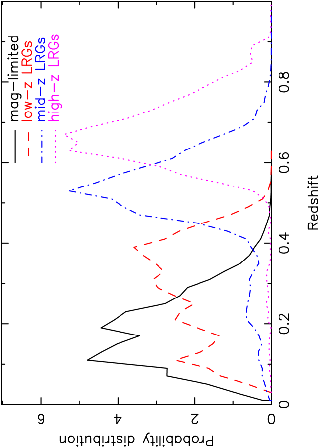
These cuts are designed to isolate the locus of early-type galaxies in colour space. Low-$z$ LRG targets must be classified as galaxies by the star-galaxy separation algorithm described in Section 3.1.6 (the fraction of stars targeted is $\sim 1\%$). Figure 3 displays the redshift distribution of targets selected in each 2dFLenS sample. The low-$z$ LRGs span redshift range $0.05<z<0.5$; the mean and standard deviation of the redshift distribution is $0.29\pm 0.12$.

Figure 3: Distribution of successful redshifts within each 2dFLenS target class. The black solid, red dashed, blue dot-dashed and magenta dotted lines show the magnitude-limited, low-$z$, mid-$z$ and high-$z$ LRG samples, respectively.

3.2.2 Mid-redshift sample

The mid-$z$ LRG sample in 2dFLenS was selected using magnitude and colour cuts similar to those employed by the BOSS ‘CMASS’ sample (Dawson et al. 2013):

$$17.5<i_{S}<19.9,$$ (15)

$$r_{S}-i_{S}<2,$$ (16)

$$d_{\perp}>0.55,$$ (17)

$$i_{S}<19.86+1.6\,(d_{\perp}-0.8).$$ (18)

A mid-$z$ LRG target must be classified as a galaxy by the star-galaxy separation algorithm, and not already be selected for the low-$z$ LRG sample. The redshift distribution of mid-$z$ LRGs is displayed as the blue dot-dashed line in Figure 3. The majority of the objects are distributed in the redshift range $0.4<z<0.8$, with a tail to lower redshifts $z<0.4$. The mean and standard deviation of the redshift distribution is $0.50\pm 0.14$. These values are comparable to those obtained by BOSS-CMASS, although the target densities of the two surveys are somewhat different, as discussed below.

3.2.3 High-redshift sample

The high-$z$ LRG sample in 2dFLenS was selected using joint optical and infra-red magnitude and colour cuts (Prakash et al. 2015) similar to those used to define the eBOSS LRG sample (Dawson et al. 2016):

$$(r-W1)>2\,(r-i),$$ (19)

$$r-i>0.98,$$ (20)

$$i-z>0.6,$$ (21)

$$19.9<i<21.8,$$ (22)

$$z<19.95.$$ (23)

A high-$z$ LRG target must not already be in the 2dFLenS low-$z$ or mid-$z$ samples. We do not apply size-based star-galaxy separation to this sample; the optical-infrared colour cut in Equation 19 is very effective for this purpose (Prakash et al. 2015). The redshift distribution of high-$z$ LRGs is displayed as the magenta dotted line in Figure 3. The high-$z$ LRGs span redshift range $0.5<z<0.9$; the mean and standard deviation of the redshift distribution is $0.67\pm 0.10$.

3.2.4 Size cut

The resulting catalogue of selected LRG galaxies was larger than the number of available 2dF-AAOmega fibres. Given this, and in order to homogenize the target density in the presence of variable seeing, we applied a size cut to the low-$z$ and mid-$z$ LRG samples such that ${\tt FLUX\_RADIUS}>4\,{\rm pixels}=0.86\,{\rm arcsec}$. We do not apply this cut to the high-$z$ LRG sample.

3.2.5 Target densities

The average target densities of the (low-$z$, mid-$z$, high-$z$) LRG samples selected across the 975 ATLAS fields were $(29,65,32)$ deg^-2. The total density was therefore a good match to the density of AAT fibres on the sky ($\approx 120$ deg^-2). The target densities in the RCS2 and CFHTLS regions were similar for the low-$z$ and mid-$z$ LRG samples, but approximately twice as high for the high-$z$ sample due to the deeper optical data. For comparison, the target densities in the SDSS (BOSS-LOWZ, BOSS-CMASS, eBOSS-LRG) samples are $(54,94,60)$ deg^-2 (Anderson et al. 2014, Dawson et al. 2016) and therefore our LRG samples are roughly a factor of 2 less dense than SDSS. This difference is driven by a combination of the size cut (Section 3.2.4), and uncertainties in photometric calibration (Section 3.6).

3.3 Magnitude-limited sample selection

3.3.1 Extended-source sample

The extended-source magnitude-limited sample, designed to facilitate direct source classification and photo-$z$ calibration, was selected by randomly sub-sampling objects in the optical catalogues subject to the following rules:

• Targets are restricted to the magnitude range $17<r<19.5$.

• In order to increase the number of bright galaxies in the sample given the steepness of the source counts, the probability of selecting a target was increased by a factor of 2 with every magnitude brighter.

• If the randomly-chosen object was already selected in another target class, this information was stored and the target was also included in the complete sample.

• Objects were classified as galaxies by the star-galaxy separation algorithm described in Section 3.1.6.

Magnitude-limited targets were assigned lower priority than LRG targets when allocating fibres in each field, such that the number varied in anti-correlation with the angular clustering of the LRG sample.

3.3.2 Point-source sample

In the 15B semester, a new set of photo-$z$ calibration targets was included in 2dFLenS observations. By checking the star-galaxy separation, we realized that the point-source sample clearly contained unresolved galaxies, which we did not want to miss for the direct photo-$z$ calibration. We further wanted to measure the object class composition of objects with colours which did not clearly correspond to isolated single stars, such as QSOs, hot subdwarfs and white dwarfs, M-dwarf/white-dwarf binaries and objects with apparently unusual colours. We thus added to the target catalogue randomly-selected objects from the point-source sample, whose colours did not clearly indicate a regular FGKM star (see Wolf et al. 2016).

3.4 Spare fibre sample selection

Wide-area spectroscopic surveys allow efficient follow-up of rare, sparsely-distributed classes of objects whose spectra would be difficult to obtain otherwise. We included several such samples in the 2dFLenS target pool.

3.4.1 Red nugget sample

The red nugget spare-fibre sample comprised Early-Type Galaxies (ETGs) at $z<1$ with effective radii $R_{e}$ and stellar masses $M_{*}$ similar to compact ETGs at $z\sim 2$ ($\log{M_{*}}>11$ and $R_{e}<2$ kpc; van Dokkum et al. 2008, Damjanov et al. 2009). We therefore chose targets that satisfied the low-$z$ or mid-$z$ LRG colour cuts but failed the size-based star-galaxy separation described in Section 3.2.4. Instead, we used the optical-infrared colour for star-galaxy separation (Equation 19), supplementing the main 2dFLenS LRG sample with objects that possessed LRG colours but would be classified as stars based on size. Since the high-$z$ LRG sample already used optical-infrared colour, red nugget targets were not added to this sample. All targets were eyeballed to remove objects affected by artefacts or close neighbours which may contaminate the WISE photometry. A total of $631$ unique red nugget spectra were observed.

The abundance of red nuggets at $z<1$ remains controversial. Using SDSS, Taylor et al. (2010) found zero ETGs in the redshift range $0.066<z<0.12$ that had sizes and masses comparable to red nuggets at $z\sim 2$. However, in the WINGS ($0.04<z<0.07$; Valentinuzzi et al. 2010) and PM2GC ($0.03<z<0.11$; Poggianti et al. 2013) surveys of low-redshift clusters, a couple of hundred red nugget analogues were found with number densities comparable to that of red nuggets at $z\sim 2$. In the COSMOS field, the number density of compact ETGs is also similar to that observed at high redshift and remains constant in the range $0.2<z<0.8$ (Damjanov et al. 2015). The 2dFLenS red nugget sample will provide another measurement of the number density and a significant increase in the number of $z<1$ red nuggets with spectra.

3.4.2 Other samples

We observed a small number of other spare-fibre targets, drawn from pools of strong gravitational lensing system candidates and Brightest Cluster Galaxies selected from the XMM Cluster Survey (XCS, Mehrtens et al. 2012) and the South Pole Telescope (SPT, Bleem et al. 2015) datasets.

3.5 Flux calibrator sample selection

Where $u$-band optical imaging data was available, three flux calibrators per AAT field were included in the 2dFLenS sample using an F-star selection (Yanny et al. 2009):

$$-0.7<0.91\,(u_{S}-g_{S})+0.415\,(g_{S}-r_{S})-1.28$$

$$<-0.25,$$ (24)

$$0.4<u_{S}-g_{S}<1.4,$$ (25)

$$0.2<g_{S}-r_{S}<0.7,$$ (26)

$$17<g_{S}<18.$$ (27)

Flux calibrators must also be classified as stars by the star-galaxy separation algorithm described in Section 3.1.6. We used the F-star spectra (where available) during the data reduction process to determine a mean sensitivity curve and zero-points for flux calibration of 2dFLenS spectra.

3.6 Photometric calibration challenges

When the VST surveys were conceived, ATLAS and KiDS were designed to facilitate precision-level photometry through overlap matching; the tiling strategies include a half-field-of-view shift between the two surveys. KiDS and ATLAS were anticipated to be observed in parallel with matched data acquisition rates such that the surveys could be used in tandem for high-precision photometry. However, in practice ATLAS progress has greatly exceeded that of KiDS. Therefore, given that the overlapping area between ATLAS pointings is insufficient to calibrate the photometric variation between fields, we are left with a significant challenge to improve ATLAS photometric calibration beyond the first-order process described in Section 3.1.1.

Shanks et al. (2015) advocate using APASS data to improve zeropoint-calibration for ATLAS beyond the ESO nightly standards. We investigated this approach, but found that the low number of objects in the APASS catalogues that were unsaturated in the ATLAS imaging was unlikely to improve our zeropoint-calibration beyond our already improved SDSS-calibration. Shanks et al. (2015) also advocate using stellar locus regression (SLR) in colour-colour space, which we also investigated. Here we compared the colours of Pickles (1998) standard stars to the colours of objects selected in our clean stellar catalogue (described in Section 3.1.6). We derived linear shifts in colour to minimise the offset between the two distributions. Whilst this provided accurate colours for all objects in the catalogue, using SLR to improve the accuracy of measured magnitudes requires fixing of the photometry in one ‘pivot’ band. We chose this pivot band in each field by minimizing the variance in the linear offsets applied to the other bands. Whilst on average this is the most optimal method to select a pivot band, on an individual field basis, this could well be the wrong choice.

The choice of an incorrect ‘pivot’ band can have a significant impact on LRG target selection, which depends on both colour and magnitude. We therefore decided only to apply SLR corrections to fields that were significant outliers in terms of the average value of $c_{\perp}$ (Equation 4) measured for galaxies with $16<r<19.6$. We selected $2\%$ of the fields that have an average $c_{\perp}$ more than $2\sigma$ away from the mean $c_{\perp}$ for the full survey. The application of our SLR magnitude correction resulted in an acceptable average value of $c_{\perp}$ for all but two of these fields, both of which were found to have a high level of artefacts which required manual masking.

Despite our efforts to achieve a good photometric calibration for ATLAS data, a full solution will require a joint re-analysis with KiDS, which has only recently acquired sufficient areal coverage to facilitate this process. For now, our ATLAS dataset still contains significant photometric systematics which affect our LRG target selection. In Section 5.1.1 we describe the mitigation of these effects in our clustering analysis, in which we are able to marginalize over these systematics with minimal impact on our scientific results.

4 Spectroscopic observations

4.1 2dF-AAOmega system and observing set-up

The 2dFLenS observational project was performed at the Anglo-Australian Telescope using the 2dF-AAOmega instrumentation. The 2dF system (Lewis et al. 2002) is a multi-fibre positioner consisting of two field plates mounted at the AAT prime focus, whose position may be exchanged using a tumbling mechanism. Whilst observations are performed using one plate, fibres for the subsequent observation may be configured on the other plate using a robot positioner. A maximum of 392 science fibres and 8 guide fibre bundles can be positioned over a circular field-of-view with a diameter of two degrees. The angular diameter of each fibre on the sky is 2 arcsec. The physical size of the magnetic buttons on which fibres are mounted implies that fibres cannot be positioned more closely together than 30 arcsec, and the probability of successfully allocating fibres to each member of a pair of galaxies decreases with pair separations below 2 arcmin.

Optical fibres (of length 38m) carry the light from the telescope prime focus to the AAOmega spectrograph. AAOmega is a bench-mounted spectrograph consisting of blue and red arms split by a dichroic (Saunders et al. 2004, Sharp et al. 2006). 2dFLenS utilizes the 580V and 385R AAOmega volume phase holographic gratings in the blue and red arms respectively, providing a uniform resolving power of $R\approx 1300$. The total wavelength range of each observation was 3700 to 8800Å, and we used the standard AAOmega dichroic with a wavelength division of 5700Å.

For each observation, target ‘field files’ were prepared consisting of the positions of science targets (with assigned priorities), potential fiducial (guide) stars to align the field accurately, and potential blank sky positions to sample the sky background to be subtracted during data reduction. The 2dF configure software was used to generate configuration files from these target lists. This software allocates the fibres using a simulated annealing algorithm (Miszalski et al. 2006), such that all targets in each successive priority band are preferentially allocated, and outputs a configuration file which was utilized by the 2dF positioner.

The 2dFLenS field files for each pointing typically consisted of 600 science targets, 100 potential guide stars and 100 blank sky positions, of which a subset of approximately 360, 8 and 25, respectively, are allocated for observation. In the software configuration process we used the following science target priorities (highest to lowest): flux calibrators (${\tt priority}=9$), spare fibre targets (8), low-$z$ LRGs (7), mid-$z$ LRGs (6), high-$z$ LRGs (5), and magnitude-limited sample (4). In practice, the numbers in each priority band imply that all targets with ${\tt priority}\geq 6$ and most targets with ${\tt priority}=5$ were observed. Flux calibrators and spare fibre targets constitute small samples (typically 3 and 5 objects per field, respectively), and were therefore accorded the highest priority to ensure they were observed.

Fibre placement by the 2dF robot positioner requires $\sim 40$ minutes for each field, for typical 2dFLenS configuration geometries. This duration specifies the minimum integration time for the observations. In order to maximize the areal coverage of the survey we fixed the integration time of each observation close to this limit: 45 minutes split into three 15-minute exposures to assist with cosmic-ray rejection. The observing sequence for each telescope pointing also included a standard fibre flat field (with exposure time 7 seconds) and arc exposure for wavelength calibration (45 seconds). Including field acquistion, CCD read-out and other overheads, observations of each 2dFLenS pointing could be completed in 1 hour. We also acquired ‘dome flat’ fields for calibration purposes, whose use is described in Section 4.3.

4.2 Guide star and blank sky positions

We selected guide stars for 2dFLenS observations from 2MASS (Skrutskie et al. 2006), to which the astrometry of our input imaging catalogues is tied. A cross-match with the UCAC4 catalogue (Zacharias et al. 2013) was used to check that potential guide stars have acceptably low proper motion and magnitudes within an appropriate range. In detail, guide stars satisfied the following criteria:

• UCAC4 $f$-band magnitude in the range $13.55<m_{f}<14.5$

• Error in this magnitude less than $0.3$ mag

• Measured proper motion $<0.02$ arcsec yr^-1

• Positional uncertainty $<0.1$ arcsec

• Offset in 2MASS-UCAC4 match $<0.5$ arcsec

All guide star candidates were visually inspected using the web-based interface described in Section 3.1.9, and only utilized if there was clear evidence that they were not galaxies, did not have close companions and were located at the expected co-ordinates.

We determined potential blank sky locations by sampling random positions from our optical images where the position satisfied the joint criteria of containing no flux (as defined by an SExtractor segmentation image using conservative parameters ${\tt MINAREA}=2$, ${\tt THRESH}=2$ and ${\tt ANALYSIS\_THRESH}=2$) and being located at least 50 pixels (11 arcsec) from a stellar halo mask or similar flag. The minimum distance between potential sky postions was specified as 5 pixels.

4.3 Data reduction

Figure 4: Spectra of 2dFLenS LRGs with good-quality redshifts stacked by rest-frame wavelength in $\Delta z=0.1$ slices. Prominent spectral features are indicated by the vertical dotted lines.

The AAOmega data were reduced during each observing run using the 2dfdr software developed at the AAO to process the science, flat-field and arc frames. The data from the blue and red spectrograph arms for each field were reduced separately, and then spliced together into a final complete spectrum. We refer the reader to Lidman et al. (2016) for a full description of the standard data reduction process, and restrict our discussion here to one important modification: in addition to the flat-field frames that are taken with the flaps that fold in front of the 2dF corrector, we also acquired flats using a patch on the windscreen that is painted white. We refer to the former as ‘flap flats’ and the latter as ‘dome flats’.

As is standard practice in processing data taken with AAOmega, we used the flap flats to measure the trace of the fibres on the CCDs (the so-called ‘tramline map’) and to determine the profile of the fibres. We did not use the dome flats directly, since the signal-to-noise ratio in the blue is too low, but instead used them to correct the flap flats.

In more detail, we processed the dome flats and the flap flats in an identical manner and then divided the flap flat by the dome flat. The result was smoothed and then multiplied back into the flap flat. This procedure preserved the high signal-to-noise ratio of the flap flat while correcting the wavelength-dependent response of the flap flat. The technique of using one kind of flat to correct another is commonly used to process imaging data, and is often referred to as an illumination correction.

The dome flats were taken once per run for each 2dF plate. We found that acquiring dome flats more often, or for every set-up, did not result in significantly better results, since the dome flats are very stable once the absolute normalisation of fibre throughput is removed.

Using illumination corrections leads to improved data reduction quality. Systematic errors in the sky subtraction are significantly smaller, especially when the background is high, which can occur during nights when the moon is above the horizon (most of the 2dFLenS data were taken during grey time). This then allows one to splice the red and blue halves of the spectrum more accurately. Errors in the splicing can lead to a discontinuity in spectra (the so-called dichroic jump) at this wavelength. While there were several factors that led to this discontinuity, the poor illumination offered by the flap flats was the largest contributing factor.

Whilst further improvements in data reduction are possible (e.g. better modelling of the fibre profile and scattered light), the quality of the reduced data is sufficient for analyses requiring an accurate estimate of the continuum such as equivalent widths, in addition to measuring line fluxes and line centroids.

4.4 Redshift determination

Figure 5: Redshift success rate of 2dFLenS observations, defined by the fraction of spectra with redshift quality flag $\geq 3$, as a function of the cross-correlation parameter ${\rm cc}_{\rm fom}$ determined by the autoz code.

Figure 6: Comparison of good-quality 2dFLenS redshifts with the redshifts of matched objects in the 2dFGRS (left-hand panel) and GAMA (middle panel) surveys, and the redshifts of repeated objects in 2dFLenS (right-hand panel). The number of objects appearing in each plot are, from left-to-right, $6{,}384$, $3{,}224$ and $839$.

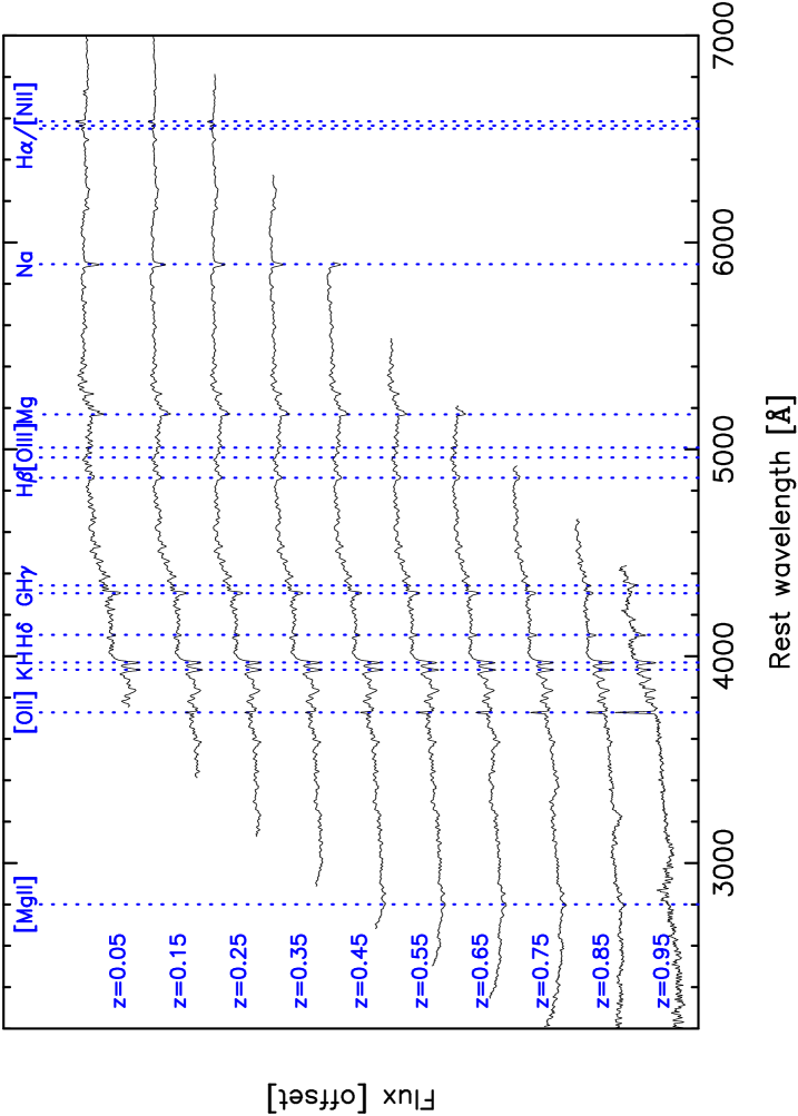
The redshifts of 2dFLenS spectra may be determined using their characteristic patterns of spectral lines in absorption and emission. The incidence of spectral lines depends on the target type: for the highest-priority LRGs, redshifts are typically derived from absorption lines including Ca H (3935Å) and K (3970Å), H$\delta$ (4103Å), G-band (4304Å), H$\beta$ (4863Å), Mg (5169Å) and Na (5895Å). Figure 4 illustrates 2dFLenS LRG spectra stacked in redshift slices of width $\Delta z=0.1$.

We used a variety of tools to determine these redshifts. Complete automation of the redshifting process is problematic due to the noisy nature of many of the spectra, and in particular the presence of artefacts such as residuals from imperfect cosmic ray, sky removal and splicing of the blue and red portions of the spectrum. Therefore, all spectra were visually inspected by 2dFLenS team members and assigned a final integer quality flag $Q$ in the range 1-6. These flag values respectively indicate: unknown redshift ($Q=1$), a possible but uncertain redshift ($Q=2$), a probably correct redshift derived from noisy data or fewer spectral features ($Q=3$), a secure redshift confirmed by multiple spectral features ($Q=4$), and a spectrum that is clearly not extragalactic ($Q=6$). The science analyses described in this paper use $Q=3$ and $Q=4$ spectra. The classification $Q=5$ is not used.

Three specific codes were used in the 2dFLenS redshifting process, two of which include a visualization capability which team members used to assign quality flags.

• runz (Saunders, Cannon & Sutherland 2004) is the AAO redshifting software with long-standing development spanning several AAT surveys such as 2dFGRS and WiggleZ. runz employs redshift determination from either discrete emission-line fitting or Fourier cross-correlation with a set of galaxy and stellar absorption-line templates (Tonry & Davis 1979). The runz code may be executed without user interaction, but reliable assignment of redshift quality flags requires subsequent visual inspection of each spectrum.

• autoz (Baldry et al. 2014) is a fully-automatic cross-correlation redshifting code developed for the Galaxy And Mass Assembly (GAMA) survey. In addition to a best-fitting redshift, autoz also returns a figure-of-merit ${\rm cc}_{\rm fom}$ which Baldry et al. (2014) relate to a quantitative confidence of redshift assignment.

• marz (Hinton et al. 2016) is an independent redshifting pipeline recently developed for the OzDES survey (Yuan et al. 2015). marz extends the matching algorithms of autoz to include quasar templates, and offers a web-based visualization interface through which users can assign quality flags and manually redshift spectra as needed.

Two different processes were used by 2dFLenS team members for assigning redshift quality flags to spectra. First, all reduced 2dFLenS fields were passed through the autoz code, and the results were captured in an input file which may be visually inspected using runz. The second possible process was to use marz for redshifting.

Possible redshifting errors and variations between 2dFLenS team members in the optimism of redshift quality-flag assignment were mitigated by subsequent inspection of borderline cases and potential blunders. In detail, all spectra flagged as bad-quality redshifts with ${\rm cc}_{\rm fom}>5$, or good-quality redshifts with ${\rm cc}_{\rm fom}<3.5$, were checked for potential blunders. Figure 5 illustrates the relation between the fraction of spectra assigned quality flags $Q\geq 3$, and the ${\rm cc}_{\rm fom}$ values assigned by the autoz code.

In order to check the reliability of assigned redshifts, we compared 2dFLenS redshifts with external surveys (2dFGRS and GAMA) where available, and also with repeat redshifts resulting from multiple observations of a field. Figure 6 illustrates the results of these comparisons. Excluding outliers, the mean and standard deviation of the quantities $z_{\rm 2dFLenS}-z_{\rm 2dFGRS}$, $z_{\rm 2dFLenS}-z_{\rm GAMA}$ and $z_{\rm 2dFLenS,obs1}-z_{\rm 2dFLenS,obs2}$ are $(-4.4\pm 10.0)\times 10^{-4}$, $(-9.8\pm 8.5)\times 10^{-4}$ and $(0.2\pm 8.1)\times 10^{-4}$, respectively, consistent with zero difference in each case. The outlier fractions in these cases are $0.9\%$, $1.3\%$ and $3.1\%$, respectively, which are negligible (and mostly consist of $Q=3$ spectra).

Redshifts are initially corrected to the heliocentric frame, and then shifted to the rest-frame of the Cosmic Microwave Background (CMB) radiation (Fixsen et al. 1996). Our data catalogues and clustering measurements are hence presented in the CMB frame.

4.5 Survey status

Figure 7: Illustration of the distribution of large-scale structure in 2dFLenS, generated by projecting the galaxy positions by right ascension and co-moving distance, indicated by the black points. The blue points in the inset display on the same scale the earlier 2dFGRS dataset (Colless et al. 2001) obtained by the AAT.

2dFLenS observations utilized $53.0$ allocated AAT nights and $3.0$ Director’s nights between 17 Sep 2014 and 5 Jan 2016. This corresponded to a total of $465.5$ potential observing hours, of which $293.6$ hrs ($63\%$) was clear, $161.8$ hrs ($35\%$) was lost to bad weather and $10.1$ hrs ($2\%$) was lost to instrumentation fault. During this time we observed 275 out of the 324 defined 2dFLenS AAT pointing centres, with 18 additional re-observations due to poor initial observing conditions. Figure 2 illustrates the final status of the survey coverage, mapping a total area of 731 deg².

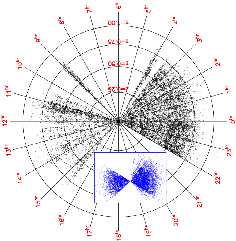
These observations yielded a total of $70{,}079$ good-quality redshifts, including $40{,}531$ LRGs and $28{,}269$ in the magnitude-limited sample. Table 3 lists the total number of observed redshifts in each target class. Figure 7 presents a projection of the positions of good-quality 2dFLenS redshifts in comparison with earlier 2dFGRS observations in the same field, illustrating the extension of the large-scale structure sample to redshift $z=0.9$.

Table 3: Number of targets observed, good redshifts obtained and the stellar fraction of those redshifts for each 2dFLenS sample. The second row adds dual-use objects to the first row, that were selected for the magnitude-limited sample but flagged for observation in different target classes. The lower half of the table lists the number of galaxies utilized in the clustering measurements described in Section 7, in redshift bins $0.15<z<0.43$ and $0.43<z<0.7$.

Target class	Spectra	Good redshifts	Stellar fraction
Complete mag-lim	$30{,}931$	$28{,}269$	$9\%$
(Including other classes)	$(31{,}864)$	$(29{,}123)$	$(9\%)$
Low-$z$ LRG	$15{,}004$	$14{,}252$	$2\%$
Mid-$z$ LRG	$32{,}032$	$19{,}376$	$8\%$
High-$z$ LRG	$18{,}116$	$6{,}903$	$6\%$
Flux calibrator	$819$	$819$	$100\%$
Spare fibre	$654$	$460$	$14\%$
Total	$97{,}556$	$70{,}079$	$8\%$
$0.15<z<0.43$ LRGs KiDS-S		$8{,}473$
$0.15<z<0.43$ LRGs KiDS-N		$3{,}556$
$0.43<z<0.7$ LRGs KiDS-S		$13{,}402$
$0.43<z<0.7$ LRGs KiDS-N		$4{,}036$

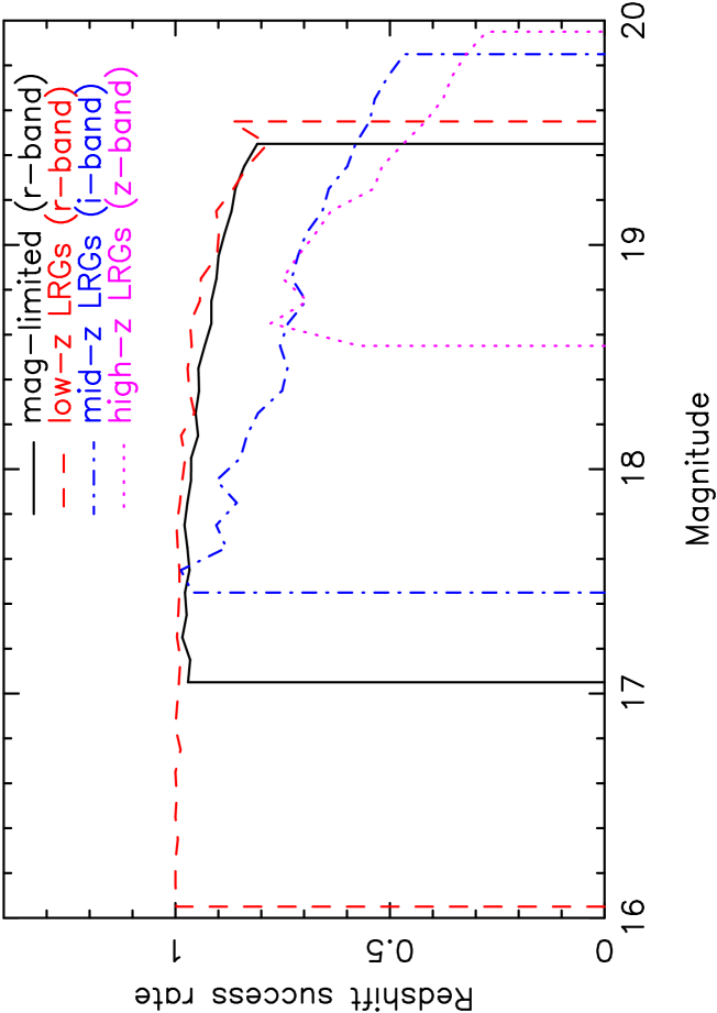
The redshift completeness of 2dFLenS pointings (i.e., the fraction of spectra with $Q\geq 3$) displays considerable variation between fields driven primarily by the observing conditions (cloud cover and seeing), and secondarily by airmass, with mean and standard deviation $71\pm 15\%$. Figure 8 displays the redshift success ($Q\geq 3$) rate for each 2dFLenS target class, as a function of the magnitude in the primary band for each selection. The average redshift success rate for the magnitude-limited, low-$z$ LRG, mid-$z$ LRG and high-$z$ LRG samples was $91\%$, $95\%$, $61\%$ and $38\%$, respectively, with a gradual decline in the success rate with fainter magnitudes.

Figure 8: Redshift success rate of 2dFLenS observations for each target class, as a function of the magnitude in the primary selection band in each case. The black solid, red dashed, blue dot-dashed and magenta dotted lines show the magnitude-limited sample ($r$-band), the low-$z$ LRG sample ($r$-band), the mid-$z$ LRG sample ($i$-band) and high-$z$ LRG sample ($z$-band), respectively.

5 Selection function

The selection function of a galaxy redshift survey describes the variation in the expected mean number density of galaxies, at 3D co-moving co-ordinate $\vec{r}$, in the absence of clustering. An accurate determination of the selection function is essential for estimating the galaxy clustering statistics, which quantify fluctuations relative to the mean density. Our model for the selection function of the 2dFLenS LRG samples considers angular fluctuations in the density of the parent target catalogue on the sky, the variation of the spectroscopic redshift completeness of each AAOmega pointing with observing conditions, and the redshift distribution of each target class together with its coupling to the completeness.

We derived selection functions and performed clustering measurements for two survey regions whose coverage is illustrated in Figure 2: KiDS-South (KiDS-S) and KiDS-North (KiDS-N). The KiDS-S analysis region is delineated by the boundaries listed in Table 1, and the KiDS-N region includes both the stripe of 2dFLenS pointings in the NGC area visible in Figure 2 and the RCS1111 region, but excludes CFHTLS W1.

5.1 Angular selection function

5.1.1 Parent target catalogue

As described in Section 3.6, field-to-field variations in the photometric accuracy of our ATLAS data reductions, of the order $0.05-0.1$ magnitudes, imprint significant systematic fluctuations in the number of selected LRG targets. The situation is illustrated by Figure 9, which displays the variation in the 1 deg fields of the number density of the three 2dFLenS LRG samples in the KiDS-S region. If left uncorrected, these fluctuations would cause significant systematic errors in the measured clustering. Similar effects are observed in the KiDS-N region.

Figure 9: Greyscale map showing the number of LRG targets selected in each ATLAS field in the KiDS-S region, relative to the mean. Significant field-to-field variations are apparent, resulting from photometric zero-point errors. The $x$- and $y$-axes plot separation in degrees from the field centre.

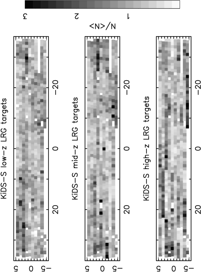
In order to mitigate this effect we adopted a conservative approach to the clustering analysis in which we marginalized over the unknown mean (unclustered) number density in each field, constrained by the observed number. For each clustering statistic we generated an ensemble of measurements corresponding to different angular selection functions. Each realization of the selection function was produced by sampling the density $\lambda$ in each ATLAS field from a probability distribution determined by the observed number of targets $N$ in that field. Assuming Poisson statistics the probability distribution is given by

$$P(\lambda|N)\propto P(N|\lambda)\,P(\lambda)=\lambda^{N}\,e^{-\lambda}/N!.$$ (28)

For large $N$, this distribution is approximated by a Gaussian with mean and variance equal to $N$. We further increased the variance of $P(\lambda)$ by adding in quadrature the contribution from angular clustering. The variance of galaxy counts-in-cells can be related to an integral of the galaxy angular correlation function $w(\theta)$ over the cell area $A$ through

$$\langle(N-\langle N\rangle)^{2}\rangle=\langle N\rangle+\langle N\rangle^{2}\frac{\int_{\rm cell}\int_{\rm cell}w(\theta)\,dA_{1}\,dA_{2}}{A^{2}}.$$ (29)

We used the moments of BOSS galaxy counts in 1 deg² cells to calibrate the final fraction in Equation 29, which has the value $\approx 0.04$, although varying this value does not significantly affect our results. The clustering contribution agrees with that calculated from our own final $w(\theta)$ measurements (using equations 1 and 2 in Blake & Wall 2002).

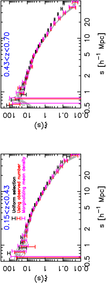
With this ensemble of selection functions and derived clustering measurements in place, we used their mean as our final determination of each statistic, and added their covariance as a systematic error contribution. This process is illustrated by Figure 10 for the case of the 2-point correlation function $\xi(s)$ in the KiDS-S region. Measurements assuming a uniform selection function, neglecting the systematic variations apparent in Figure 9, contain systematic error on large scales, which may be corrected using the observed number density distribution as the angular selection. Marginalizing over the unknown mean density in each field produces an ensemble of clustering measurements whose variation defines a systematic error contribution. Importantly, we note that the magnitude of this systematic error is significantly less than the statistical error – by typically an order of magnitude – for all the clustering measurements considered in this paper. Therefore, whilst we always perform this marginalization process, it does not have a significant impact on our results.

Figure 10: Illustration of our clustering analysis marginalizing over the unknown mean galaxy density in each ATLAS field, for the case of the 2-point correlation function $\xi(s)$ in the KiDS-S region in the two redshift ranges $0.15<z<0.43$ (left panel) and $0.43<z<0.7$ (right panel). The black data points are measurements assuming a uniform selection function, neglecting the systematic target density variations, and contain large-scale systematic errors. These may be corrected using the observed number density in each tile as the angular selection, which produces the red data points. The set of grey lines is an ensemble of clustering measurements in which the selection function is statistically sampled from a distribution defined by the observed number and clustering strength. The magenta data points show the mean of this distribution, adding the density systematic error in quadrature to the original error. Measurements for the different cases are slightly shifted along the $x$-axis for clarity.

5.1.2 Redshift completeness

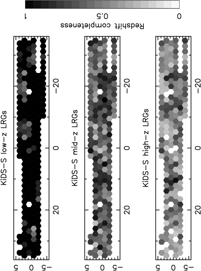
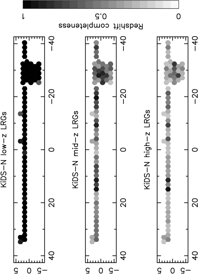
LRG targets were uniquely assigned to the closest AAT field centre in our pointing grid, producing a set of hexagonal survey sectors. We modelled the variation in the angular selection function due to incompleteness in redshift determination using the ratio of good-quality redshifts to targets within each of these sectors. These redshift completeness maps are displayed in Figure 11 for the low-$z$, mid-$z$ and high-$z$ LRG samples within the KiDS-S and KiDS-N survey regions. The low-$z$ LRG follow-up is highly complete, but the mid-$z$ and high-$z$ samples are imprinted with significant completeness variations driven by AAT observing conditions. We neglected any variation in the redshift completeness across the 2-degree field-of-view (which may be imprinted by either rotational mis-alignments in acquistion or enhanced chromatic aberrations towards the edges of the field). This variation was lower than $\sim 10\%$ for 2dFLenS observations.

Figure 11: Greyscale map showing the redshift completeness of 2dFLenS observations in the KiDS-S (top 3 rows) and KiDS-N (bottom 3 rows) regions. The $x$- and $y$-axes plot separation in degrees from the field centre.

5.2 Radial selection function

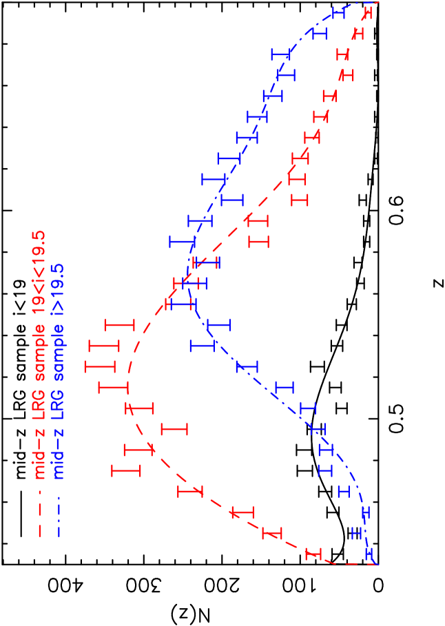
We determined the redshift dependence of the selection function by fitting parametric models (using Chebyshev polynomials) to the empirical redshift distributions $N(z)$ of each LRG sample. We determined the order of the polynomial via a combination of information criteria considerations and visual inspection.

Our model included the coupling between $N(z)$ and the angular redshift completeness, such that our selection function is not separable into angular and radial pieces. This coupling arises because in poorer observing conditions, corresponding to areas of lower total redshift completeness, successful redshifts are preferentially obtained for sources with brighter magnitudes (see Figure 8), which are preferentially located at lower redshifts. In detail, we fitted $N(z)$ functions for LRG samples in bands of apparent magnitude, and constructed the model $N(z)$ within each survey pointing using the magnitude distribution of galaxies with successful redshifts within that pointing. Figure 12 shows example $N(z)$ fits for the mid-$z$ LRG sample.

Figure 12: The redshift distribution of the mid-$z$ LRG sample in $i$-band magnitude bands, together with Chebyshev polynomial fits.

5.3 Redshift bins

The low-$z$, mid-$z$ and high-$z$ 2dFLenS LRG samples overlap in redshift, as illustrated by Figure 3. We combined the LRG samples into two independent redshift bins: $0.15<z<0.43$ and $0.43<z<0.7$, weighting the selection function of each sample by the relative target numbers. The choice of these bins was motivated by intended comparisons and combinations with the LOWZ and CMASS samples of BOSS (Dawson et al. 2013), for example, to extend the analysis of $E_{G}$ presented by Blake et al. (2016) in these redshift bins. Clustering measurements for 2dFLenS LRGs in these two redshift bins will be presented in Section 7.

We computed the effective redshift of the selection functions in each redshift bin as

$$z_{\rm eff}=\sum_{\vec{r}}z\,\left(\frac{n_{g}(\vec{r})P_{g}}{1+n_{g}(\vec{r})P_{g}}\right)^{2},$$ (30)

where $n_{g}(\vec{r})$ is the mean galaxy number density in each grid cell $\vec{r}$ and $P_{g}$ is the characteristic galaxy power spectrum amplitude, which we evaluated at a scale $k=0.1\,h$ Mpc^-1 using the fiducial matter power spectrum and galaxy bias factors specified in Section 7. We obtained effective redshifts $z_{\rm eff}=0.31$ and $0.56$ in the two bins $0.15<z<0.43$ and $0.43<z<0.7$.

5.4 Fibre collisions

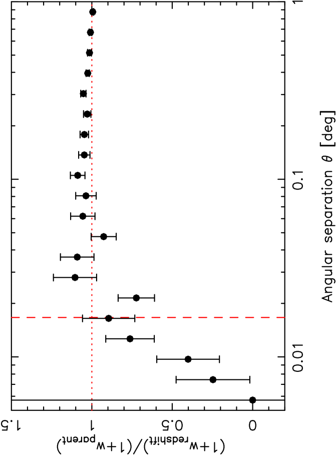
The minimum separation of the optical fibres of the 2dF spectrograph is 30 arcsec, and there is a diminishing probability of observing in a single pointing both members of a close pair of parent galaxies separated by an angular distance of less than 2 arcmin. This deficit of close angular pairs in the redshift catalogue, known as ‘fibre collisions’, artificially suppresses the measured galaxy correlation function on small scales. We assess the deficit of close angular pairs in Figure 13 by plotting the ratio $(1+w_{z})/(1+w_{p})$ as a function of angular separation $\theta$, where $w_{z}$ and $w_{p}$ are the angular correlation functions of the redshift and parent catalogues, respectively. We measured the angular correlation functions by applying the Landy-Szalay estimator (Landy & Szalay 1993) to the positions of the data sources $D$ and a catalogue of random sources $R$ which sample the survey selection function:

$$w(\theta)=\frac{DD(\theta)-2\,DR(\theta)+RR(\theta)}{RR(\theta)}.$$ (31)

Significant effects are only detectable at the very smallest scales $\theta<1$ arcmin, and we do not correct for them in our analysis.

Figure 13: The ratio of the angular correlation functions of the 2dFLenS parent and redshift catalogues, indicating the fraction of close pairs surviving the restrictions of fibre collisions as a function of angular separation. Jack-knife errors are plotted. The vertical dashed line corresponds to a separation of 1 arcmin, below which fibre collision effects are detectable. The ratio is driven to values greater than 1 at moderate angular scales by stellar contamination in the parent catalogue, which reduces the value of $w_{\rm parent}$ compared to $w_{\rm redshift}$.

6 Mock catalogues

We determined the covariance of our 2dFLenS clustering statistics, and their joint covariance with overlapping measurements of galaxy-galaxy lensing and cosmic shear, using a set of mock catalogues created from a large suite of N-body simulations which included a self-consistent computation of gravitational lensing.

6.1 SLICS catalogues

Our mocks are built from the SLICS (Scinet LIght Cone Simulations) series (Harnois-Deraps & van Waerbeke 2015). At the time of writing, SLICS consisted of 930 N-body simulations created with the CUBEP³M code (Harnois-Deraps et al. 2013) using a WMAP9+BAO+SN cosmological parameter set: matter density $\Omega_{m}=0.2905$, baryon density $\Omega_{b}=0.0473$, Hubble parameter $h=0.6898$, spectral index $n_{s}=0.969$ and normalization $\sigma_{8}=0.826$. The box-size of the simulations is $L=505\,h^{-1}$ Mpc, in which the non-linear evolution of $1536^{3}$ particles is followed inside a $3072^{3}$ grid cube.

For each simulation, the density field was output at 18 redshift snapshots in the range $0<z<3$. The gravitational lensing shear and convergence is computed at these multiple lens planes using the flat-sky Born approximation, and a survey cone spanning 60 deg² is constructed by pasting together these snapshots. In this process, the planes were randomly shifted and the direction of the collapsed dimension was changed in order to minimize residual correlations (see Harnois-Deraps & van Waerbeke 2015 for a complete description of the light cone construction). A spherical over-density halo finder was executed on the particle data during the simulation run, producing dark matter halo catalogues containing properties such as the mass, position, center-of-mass velocity and 3-dimensional velocity dispersion. These were then post-processed in order to select only those that belonged to the light-cone geometry, self-consistently reproducing the rotation and random shift imposed on the lens planes.

We used these simulation data products to build self-consistent mock catalogues for overlapping cosmic shear and galaxy redshift surveys, including realistic source and lens number densities, redshift distributions and sampling of the density field. We produced mocks for two distinct cases. First, we neglected the variation of the angular selection function and generated 930 mocks, each of area 60 deg². Secondly, we tiled together the individual simulations to cover the area of our KiDS-N and KiDS-S regions (in a flat-sky approximation). The resulting tiled datasets could accommodate 65 mock catalogues using no simulated volume twice, which we sub-sampled with the realistic angular selection functions of the cosmic shear and galaxy redshift surveys.

The ensemble of 930 mocks is useful for determining the covariance of a large data vector, such as an observation including cosmic shear tomography, which can be area-scaled to match the true survey area. The 65 larger mocks, which include the full selection function, permit a more accurate determination of the covariance of the 2dFLenS clustering measurements and were used in our analysis described in Section 7.

6.2 Halo occupation distribution

We produced mock galaxy redshift survey catalogues by populating the dark matter haloes of the N-body simulations using a Halo Occupation Distribution (HOD) designed to match the measured large-scale clustering amplitude of 2dFLenS galaxies. For the purposes described here, in which the small-scale ‘1-halo’ clustering features are not important and cannot be accurately measured due to fibre collisions and low signal-to-noise ratio, we adopted a central galaxy HOD such that the probability that a dark matter halo of mass $M$ hosts an LRG transitions from 0 to 1 according to

$$P(M)=\frac{1}{2}\left[1+{\rm erf}\left(\frac{\log_{10}M-\log_{10}M_{0}}{\sigma_{\log{M}}}\right)\right],$$ (32)

where $M_{0}$ and $\sigma_{\log{M}}$ are free parameters, and we neglected satellite galaxies. After populating dark matter haloes in this manner, placing the mock galaxy at the central position of the halo and assigning it the halo’s centre-of-mass velocity, we sub-sampled the mock galaxy distribution to match the 3D selection function of the 2dFLenS galaxies in each survey region, deriving a redshift-space position. We varied the parameters $M_{0}$ and $\sigma_{\log{M}}$ to reproduce the measured 2dFLenS clustering, finding that an acceptable match was produced by the choices $M_{0}=10^{14.1}\,h^{-1}M_{\odot}$ and $\sigma_{\log{M}}=0.2$, i.e. cluster-scale halos. This value of $M_{0}$ falls at the upper end of the range found in fits to BOSS-CMASS LRGs (Guo et al. 2014), consistent with the lower number density of 2dFLenS LRGs and our neglect of the satellite contribution.

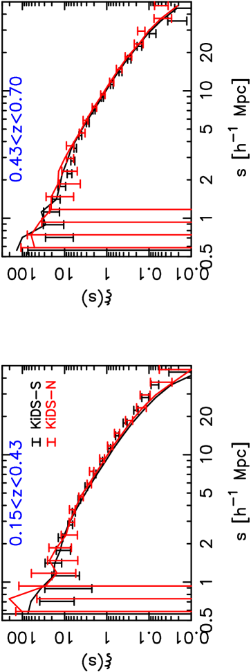
We note that the systematic photometric variations described in Section 3.6 produced an artificial increase in the survey selection function in some (small) areas, resulting in a target galaxy number density which cannot be matched by haloes selected via Equation 32. In these areas, we supplemented the mock catalogue by randomly sampling haloes with masses $M>10^{13.8}\,h^{-1}M_{\odot}$, until the target number density was matched. A comparison of the spatial correlation functions $\xi_{0}(s)$ of the data and mock catalogues is shown in Figure 14, illustrating the agreement produced by our approach.

Figure 14: The spatial correlation function $\xi_{0}(s)$ measured in the KiDS-S and KiDS-N survey regions (black and red data points) compared to similar measurements in the mock catalogues (solid lines).

6.3 Joint lensing catalogues

For science analyses requiring joint lensing and clustering mocks, we produced the mock lensing catalogues using the approach described by Joudaki et al. (2016a), which we briefly summarize here.

• We populated each simulation cone using a source redshift distribution and an effective source density matching that of the lensing survey, by Monte-Carlo sampling sources from the simulation density field.

• We assigned two-component gravitational shears $(\gamma_{1},\gamma_{2})$ to each mock source by linearly interpolating the shear fields at the source positions between the values at adjacent snapshot redshifts.

• We applied shape noise to the mock sources, drawing the noise components from a Gaussian distribution with standard deviation matching that of the lensing survey.

We note that, although sources in the cosmic shear survey dataset have optimal weights determined by the shape measurement process, we produced lensing mocks in which all sources have uniform weight, and the varying weights are absorbed into the effective source density, redshift distribution and shape noise.

7 Clustering measurements

In this Section we present clustering measurements of 2dFLenS LRGs using three statistics. First, we determined the projected correlation function $w_{p}(r_{p})$ as a function of transverse separation $r_{p}$, in which the effect of redshift-space distortion is removed by integrating along the line-of-sight direction (Section 7.1). The projected correlation function is used to estimate the bias of the galaxy sample and is also required for determining the gravitational slip statistic $E_{G}$ as a test of gravitational physics (Amon et al. 2016). We also computed two statistics which quantify the dependence of the clustering amplitude on the angle to the line-of-sight: the correlation function multipoles $\xi_{\ell}(s)$ (Section 7.2) and the power spectrum multipoles $P_{\ell}(k)$ (Section 7.3). These statistics are used to fit models for redshift-space distortion, and we also test whether consistent results are produced in Fourier space and configuration space. We converted the galaxy angular positions and redshifts into 3D co-moving space using a flat $\Lambda$CDM fiducial cosmology with matter density $\Omega_{\rm m}=0.3$.

7.1 Projected correlation function and galaxy bias

We estimated the projected correlation function of 2dFLenS galaxies by initially measuring the 2D correlation function $\xi(r_{p},\Pi)$ as a function of projected pair separation $r_{p}$ and line-of-sight separation $\Pi$ using the Landy-Szalay estimator:

$$\xi(r_{p},\Pi)=\frac{DD(r_{p},\Pi)-2\,DR(r_{p},\Pi)+RR(r_{p},\Pi)}{RR(r_{p},\Pi)}.$$ (33)

In each 2dFLenS survey region we generated a random catalogue 10 times larger than the data catalogue. In Equation 33, $DD$, $DR$ and $RR$ are the data-data, data-random and random-random pair counts in each separation bin. For a pair of galaxies with position vectors $\vec{r}_{1}$ and $\vec{r}_{2}$, mean position $\vec{r}=(\vec{r}_{1}+\vec{r}_{2})/2$ and separation vector $\vec{s}=\vec{r_{2}}-\vec{r_{1}}$, the separation bin values are defined by $\Pi=|\vec{s}.\vec{r}|/|\vec{r}|$ and $r_{p}=\sqrt{|\vec{s}|^{2}-\Pi^{2}}$.

We then determined the projected correlation function using the sum

$$w_{p}(r_{p})=2\sum_{i}\xi(r_{p},\Pi_{i})\,\Delta\Pi_{i},$$ (34)

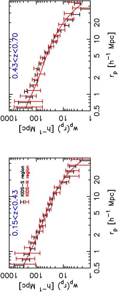
where we summed over 10 logarithmically-spaced bins in $\Pi$ from $0.1$ to $60\,h^{-1}$ Mpc. The measurements of $w_{p}(r_{p})$ for 2dFLenS galaxies in 20 logarithmically-spaced bins in $r_{p}$ from $0.5$ to $50\,h^{-1}$ Mpc are shown in Figure 15, for the two redshift ranges $0.15<z<0.43$ and $0.43<z<0.7$. Errors are obtained from the mock catalogues.

For illustrative purposes we show the fit of a single-parameter bias model to the data using a non-linear power spectrum $P_{\rm m}(k)$ computed in a fiducial cosmology. We generated $P_{\rm m}(k)$ using the non-linear corrections calibrated by Takahashi et al. (2012) as implemented by the camb software package (Lewis, Challinor & Lasenby 2000). For the purposes of this measurement we specified the cosmological parameters used to generate the model power spectrum as the maximum-likelihood (“TT+lowP”) parameters fit to Planck CMB observations and quoted in the 1st column of Table 3 in Planck collaboration (2015): physical baryon density $\Omega_{\rm b}h^{2}=0.02222$, physical cold dark matter density $\Omega_{\rm c}h^{2}=0.1197$, Hubble parameter $H_{0}=67.31$ km s^-1 Mpc^-1, spectral index $n_{\rm s}=0.9655$ and normalization $\sigma_{8}=0.829$. The best-fitting bias parameters are $b=1.84\pm 0.03$ ($0.15<z<0.43$) and $b=2.10\pm 0.03$ ($0.43<z<0.7$).

Figure 15: The projected correlation function $w_{p}(r_{p})$ for 2dFLenS LRGs in the KiDS-S and KiDS-N regions. Results are shown for two redshift ranges $0.15<z<0.43$ (left) and $0.43<z<0.7$ (right) with errors estimated using the ensemble of mock catalogues. The solid lines indicate the best fit of a single-parameter bias model in our fiducial cosmology.

7.2 Multipole correlation functions

We estimated the redshift-space correlation function $\xi(s,\mu)$ as a function of co-moving separation $s=|\vec{s}|$ and the cosine of the angle of the pair separation vector with respect to the line-of-sight towards the mean position $\vec{r}$, $\mu=|\vec{s}.\vec{r}|/|\vec{s}||\vec{r}|$, using a Landy-Szalay estimator equivalent to Equation 33. For this estimate we assigned each galaxy optimal ‘FKP’ weights (Feldman, Kaiser & Peacock 1994) defined by

$$w_{\rm FKP}(\vec{r})=\frac{1}{1+n_{g}(\vec{r})\,P_{g}},$$ (35)

where $n_{g}(\vec{r})$ is the galaxy number density at position $\vec{r}$ expected in the mean realization of the survey selection function, and $P_{g}$ is a characteristic value of the power spectrum, which we take as $P_{g}=20{,}000\,h^{-3}$ Mpc³ motivated by the power spectrum measurements presented in Section 7.3. This weighting scheme ensures equal weight per volume where the measurement is limited by sample variance ($n_{g}P_{g}\gg 1$) and equal weight per galaxy where the measurement is limited by shot noise ($n_{g}P_{g}\ll 1$). We used 9 separation bins of width $\Delta s=10\,h^{-1}$ Mpc in the range $s<90\,h^{-1}$ Mpc, and 100 angular bins of width $\Delta\mu=0.01$.

It is convenient to compress the information encoded in $\xi(s,\mu)$ into correlation function multipoles defined by

$$\xi_{\ell}(s)=\frac{2\ell+1}{2}\int_{-1}^{1}d\mu\,\xi(s,\mu)\,L_{\ell}(\mu),$$ (36)

where $L_{\ell}$ is the Legendre polynomial of order $\ell$. The linear-theory contribution to the clustering is described by a summation over terms $\ell=\{0,2,4\}$. The monopole $\xi_{0}(s)$ represents the total angle-averaged spatial correlation function; the quadrupole $\xi_{2}(s)$ encodes the leading-order redshift-space distortion signal. We estimated $\xi_{\ell}(s)$ in Equation 36 by converting the integral into a sum over $\mu$-bins.

Figure 16 displays our measurement of the multipole correlation functions for 2dFLenS data in the KiDS-S and KiDS-N regions for redshift ranges $0.15<z<0.43$ and $0.43<z<0.7$. We are able to detect the signature of redshift-space distortion via the non-zero values of the quadrupole $\xi_{2}(s)$; the hexadecapole $\xi_{4}(s)$ is consistent with zero. We overplot the best-fitting redshift-space distortion model (see Section 7.4).

We estimated the correlation function multipoles for each of the mock catalogues, and used the measurements for the ensemble of realizations to construct a covariance matrix

$${\rm Cov}_{ij}=\langle\xi_{\rm est}(i)\,\xi_{\rm est}(j)\rangle-\langle\xi_{\rm est}(i)\rangle\,\langle\xi_{\rm est}(j)\rangle,$$ (37)

where the array $\xi_{\rm est}(i)$ consists of the concatenation

$$\{\xi_{0}(s_{1}),\xi_{0}(s_{2}),...,\xi_{2}(s_{1}),\xi_{2}(s_{2}),...,\xi_{4}(s_{1}),\xi_{4}(s_{2}),...\}.$$ (38)

The corresponding correlation matrix, defined by ${\rm Cov}_{ij}/\sqrt{{\rm Cov}_{ii}\,{\rm Cov}_{jj}}$, is displayed in Figure 17 for the KiDS-S region for the redshift range $0.43<z<0.7$ (results for the other region and redshift range are similar). The off-diagonal correlations are typically low, and dominated by neighbouring separation bins. We also plot in Figure 16 the $68\%$ confidence range of the mock correlation function measurements, within which the data points generally lie.

Figure 16: The multipole correlation functions $(\xi_{0},\xi_{2},\xi_{4})$, from left-to-right, for 2dFLenS LRGs in the KiDS-S and KiDS-N regions. Results are shown for two redshift ranges $0.15<z<0.43$ (top row) and $0.43<z<0.7$ (bottom row), and scaled by $s^{2}$ for clarity of presentation. The solid red line indicates the best-fitting model and the magenta dotted lines display the mock mean and $68\%$ confidence range of mock measurements for the KiDS-S region.

Figure 17: The correlation matrix for the 2dFLenS multipole correlation functions arranged in a data vector $\xi_{\rm est}(i)=\{\xi_{0},\xi_{2},\xi_{4}\}$, derived from the mock catalogues as ${\rm Cov}_{ij}/\sqrt{{\rm Cov}_{ii}\,{\rm Cov}_{jj}}$. Results are shown for the redshift range $0.43<z<0.7$ for the KiDS-S region; they are similar for the redshift range $0.15<z<0.43$ and for KiDS-N. The labels $(30,60,90)$ denote separations in $h^{-1}$ Mpc.

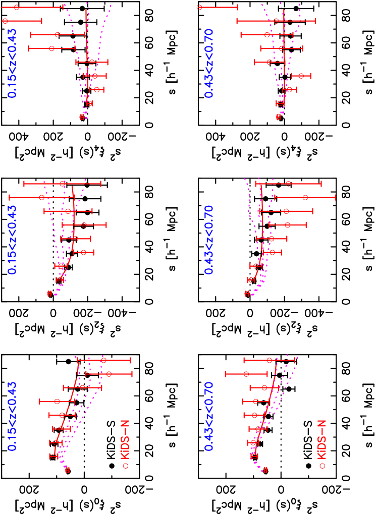
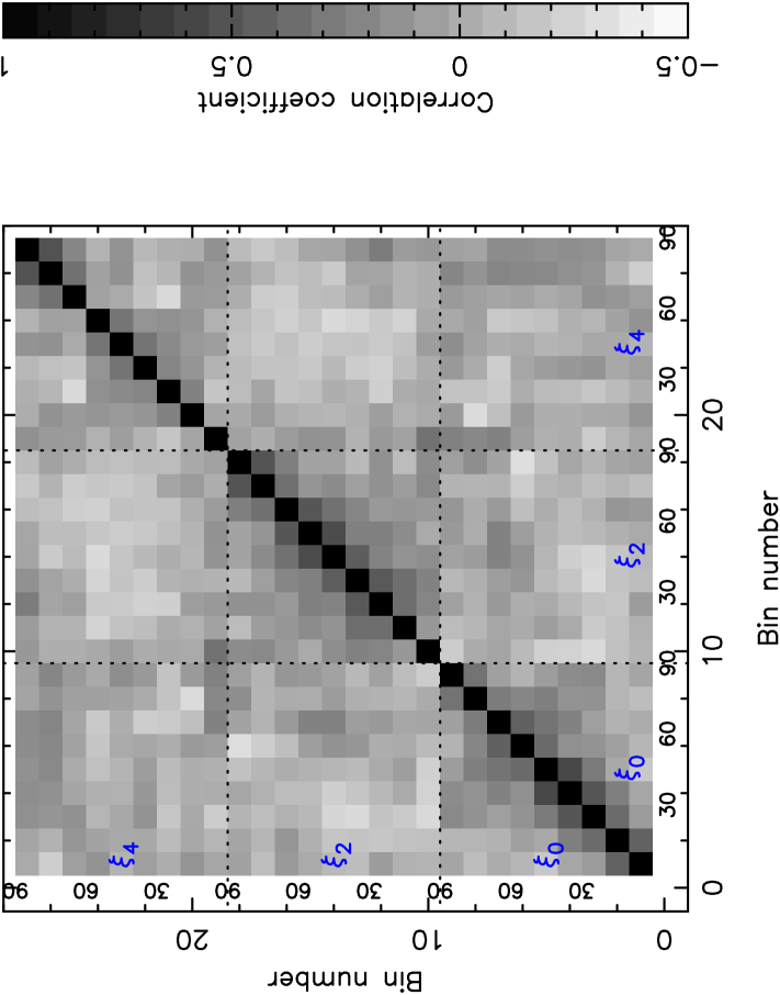
7.3 Multipole power spectra

The dependence of the galaxy clustering amplitude on the angle to the line-of-sight, including redshift-space distortion, may be quantified in Fourier space using multipole power spectra $P_{\ell}(k)$:

$$P(k,\mu)=\sum_{\ell}P_{\ell}(k)\,L_{\ell}(\mu).$$ (39)

The orthogonality of $L_{\ell}(\mu)$ implies that

$$P_{\ell}(k)=\frac{2\ell+1}{2}\int_{-1}^{1}d\mu\,P(k,\mu)\,L_{\ell}(\mu).$$ (40)

7.3.1 Power spectrum estimation

We estimated the multipole power spectra $\{P_{0}(k),P_{2}(k),P_{4}(k)\}$ using the direct Fast Fourier Transform (FFT) method presented by Bianchi et al. (2015) and Scoccimarro (2015). The use of FFTs results in a significant speed-up compared to the estimation by direct summation described earlier by Yamamoto et al. (2006), Blake et al. (2011a) and Beutler et al. (2014).

We first enclosed the survey cone within a cuboid of sides $(L_{x},L_{y},L_{z})$ and gridded the catalogue of $N$ galaxies in cells numbering $(n_{x},n_{y},n_{z})$ using nearest grid point assignment to produce a distribution $n(\vec{r})$, where $\sum_{\vec{r}}n(\vec{r})=N$. The cell dimensions were chosen such that the Nyquist frequencies in each direction (e.g. $k_{\rm Nyq}=\pi n_{x}/L_{x}$) exceeded the maximum frequency of measured power by at least a factor of 3. We then defined the weighted overdensity field

$$F(\vec{r})=w_{\rm FKP}(\vec{r})\,\left[n(\vec{r})-N\,W(\vec{r})\right],$$ (41)

where $W(\vec{r})$ is proportional to the survey selection function determined in Section 5, which describes the number of galaxies expected in each cell $\vec{r}$ in the absence of clustering assuming the normalization $\sum_{\vec{r}}W(\vec{r})=1$.

We employed the following estimators for the power spectrum multipoles (Bianchi et al. 2015, equations 6-8):

$$P_{0}(\vec{k})=\frac{1}{I}\,A_{0}(\vec{k})\,A_{0}^{*}(\vec{k})-P_{\rm noise},$$ (42)

$$P_{2}(\vec{k})=\frac{5}{2I}\,A_{0}(\vec{k})\,\left[3A_{2}^{*}(\vec{k})-A_{0}^{*}(\vec{k})\right],$$ (43)

$$P_{4}(\vec{k})=\frac{9}{8I}\,A_{0}(\vec{k})\,\left[35A_{4}^{*}(\vec{k})-30A_{2}^{*}(\vec{k})+3A_{0}^{*}(\vec{k})\right],$$ (44)

in terms of the variables

$$A_{n}(\vec{k})=\int d^{3}\vec{r}\,(\hat{\vec{k}}.\hat{\vec{r}})^{n}\,F(\vec{r})\,\exp{(i\vec{k}.\vec{r})},$$ (45)

$$P_{\rm noise}=\int d^{3}\vec{r}\,w_{\rm FKP}(\vec{r})^{2}\,n(\vec{r}),$$ (46)

$$I=N^{2}\int d^{3}\vec{r}\,w_{\rm FKP}(\vec{r})^{2}\,W(\vec{r})^{2}.$$ (47)

We determined the functions $A_{n}(\vec{k})$ by evaluating the following quantities using FFTs:

$$A_{0}(\vec{k})=\int d^{3}\vec{r}\,F(\vec{r})\,\exp{(i\vec{k}.\vec{r})},$$ (48)

$$B_{ij}(\vec{k})=\int d^{3}\vec{r}\,b_{ij}(\vec{r})\,F(\vec{r})\,\exp{(i\vec{k}.\vec{r})},$$ (49)

$$C_{ijk}(\vec{k})=\int d^{3}\vec{r}\,c_{ijk}(\vec{r})\,F(\vec{r})\,\exp{(i\vec{k}.\vec{r})},$$ (50)

where

$$b_{ij}(\vec{r})=\frac{r_{i}\,r_{j}}{r^{2}},$$ (51)

$$c_{ijk}(\vec{r})=\frac{r_{i}^{2}\,r_{j}\,r_{k}}{r^{4}}.$$ (52)

The indices $(i,j,k)$ range over $\{1,2,3\}$, where $(r_{1},r_{2},r_{3})=(x,y,z)$. In terms of these variables,

$$A_{2}(\vec{k}) = \sum_{ij}\beta_{ij}(\vec{k})\,B_{ij}(\vec{k})$$ (54)

$$= \frac{1}{k^{2}}\{k_{x}^{2}B_{xx}+k_{y}^{2}B_{yy}+k_{z}^{2}B_{zz}$$

$$+2\left[k_{x}k_{y}B_{xy}+k_{x}k_{z}B_{xz}+k_{y}k_{z}B_{yz}\right]\},$$

and

$$A_{4}(\vec{k}) = \sum_{ijk}\gamma_{ijk}(\vec{k})\,C_{ijk}(\vec{k})$$ (56)

$$= \frac{1}{k^{4}}\{k_{x}^{4}C_{xxx}+k_{y}^{4}C_{yyy}+k_{z}^{4}C_{zzz}$$

$$+4\left[k_{x}^{3}k_{y}C_{xxy}+k_{x}^{3}k_{z}C_{zzx}+k_{y}^{3}k_{x}C_{yyx}\right]$$

$$+4\left[k_{y}^{3}k_{z}C_{yyz}+k_{z}^{3}k_{x}C_{zzx}+k_{z}^{3}k_{y}C_{zzy}\right]$$

$$+6\left[k_{x}^{2}k_{y}^{2}C_{xyy}+k_{x}^{2}k_{z}^{2}C_{xzz}+k_{y}^{2}k_{z}^{2}C_{yzz}\right]$$

$$+12\,k_{x}k_{y}k_{z}\left[k_{x}C_{xyz}+k_{y}C_{yxz}+k_{z}C_{zxy}\right]\}.$$

We obtained the final power spectrum multipoles $\{P_{0}(k),P_{2}(k),P_{4}(k)\}$ by angle-averaging $P_{\ell}(\vec{k})$ in spherical shells in $\vec{k}$-space.

Our measurements of the multipole power spectra $\{P_{0},P_{2},P_{4}\}$ for the 2dFLenS KiDS-S and KiDS-N regions, for the two redshift ranges $0.15<z<0.43$ and $0.43<z<0.7$, are displayed in Figure 18. We used 10 Fourier bins of width $\Delta k=0.02\,h$ Mpc^-1 in the range $0<k<0.2\,h$ Mpc^-1. A clear detection of non-zero quadrupole $P_{2}(k)$ is again obtained, and the hexadecapole $P_{4}(k)$ is consistent with zero. We overplot the best-fitting redshift-space distortion model (see Section 7.4) convolved with the window function using the method described in the following sub-section.

Figure 18: The multipole power spectra $(P_{0},P_{2},P_{4})$, from left-to-right, for 2dFLenS LRGs in the KiDS-S (black solid circles) and KiDS-N (red open circles) regions. Results are shown for two redshift ranges $0.15<z<0.43$ (top row) and $0.43<z<0.7$ (bottom row). The solid lines indicate the best-fitting model convolved in each case with the region window function, which produces the ‘choppy’ appearance in the model.

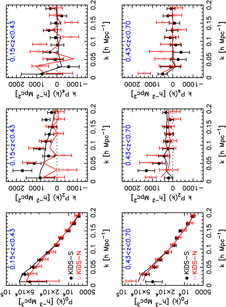
7.3.2 Convolution by the window function

The expectation value of the power spectrum estimators in Section 7.3.1 is the underlying power spectrum $P(\vec{k})$ convolved with the survey selection function. These convolutions may also be evaluated using FFTs, which we accomplished using the following scheme extending the results of the previous section:

$$P_{0,{\rm c}}(\vec{k})=\frac{1}{I}(A_{0}A_{0}^{*})_{\rm c},$$ (57)

$$P_{2,{\rm c}}(\vec{k})=\frac{5}{2I}\left[3(A_{0}A_{2}^{*})_{\rm c}-(A_{0}A_{0}^{*})_{\rm c}\right],$$ (58)

$$P_{4,{\rm c}}(\vec{k})=\frac{9}{8I}\left[35(A_{0}A_{4}^{*})_{\rm c}-30(A_{0}A_{2}^{*})_{\rm c}+3(A_{0}A_{0}^{*})_{\rm c}\right].$$ (59)

where

$$(A_{0}A_{0}^{*})_{\rm c}=\int d^{3}\vec{k}^{\prime}\,P_{\rm mod}(\vec{k}^{\prime})\,W_{0}(\delta\vec{k})\,W_{0}^{*}(\delta\vec{k}),$$ (60)

$$(A_{0}A_{2}^{*})_{\rm c}=\int d^{3}\vec{k}^{\prime}\,P_{\rm mod}(\vec{k}^{\prime})\,W_{0}(\delta\vec{k})\,\times$$

$$\sum_{ij}\beta_{ij}(\delta\vec{k})\,W_{2,ij}^{*}(\delta\vec{k}),$$ (61)

$$(A_{0}A_{4}^{*})_{\rm c}=\int d^{3}\vec{k}^{\prime}\,P_{\rm mod}(\vec{k}^{\prime})\,W_{0}(\delta\vec{k})\,\times$$

$$\sum_{ijk}\gamma_{ijk}(\delta\vec{k})\,W_{4,ijk}^{*}(\delta\vec{k}),$$ (62)

where $\delta\vec{k}=\vec{k}-\vec{k}^{\prime}$, in terms of

$$W_{0}(\vec{r})=w_{\rm FKP}(\vec{r})\,W(\vec{r}),$$ (63)

$$W_{2,ij}(\vec{r})=b_{ij}(\vec{r})\,w_{\rm FKP}(\vec{r})\,W(\vec{r}),$$ (64)

$$W_{4,ijk}(\vec{r})=c_{ijk}(\vec{r})\,w_{\rm FKP}(\vec{r})\,W(\vec{r}).$$ (65)

For reasons of further computing speed when fitting models, we re-cast this convolution as a matrix multiplication in Fourier bins of width $\Delta k=0.02\,h$ Mpc^-1:

$$P_{\rm est}(i)=\sum_{j}M_{ij}\,P_{\rm mod}(j),$$ (66)

where the arrays $P_{\rm est}(i)$ and $P_{\rm mod}(j)$ consist of the concatenation

$$\{P_{0}(k_{1}),P_{0}(k_{2}),...,P_{2}(k_{1}),P_{2}(k_{2}),...,P_{4}(k_{1}),P_{4}(k_{2}),...\}.$$ (67)

We determined the matrix $M_{ij}$ by evaluating the full convolution for a set of unit vectors. For each unit vector the model $P_{\rm mod}(\vec{k})$ is computed using Equation 39 setting a single element of Equation 67 to unity and the rest of the elements to zero.

7.3.3 Covariance matrix

We measured the power spectrum multipoles for each 2dFLenS mock catalogue, producing a series of data vectors $P_{\rm est}(i)$. We hence deduced the covariance matrix by averaging over the mocks

$${\rm Cov}_{ij}=\langle P_{\rm est}(i)\,P_{\rm est}(j)\rangle-\langle P_{\rm est}(i)\rangle\,\langle P_{\rm est}(j)\rangle.$$ (68)

The corresponding correlation matrix, defined by ${\rm Cov}_{ij}/\sqrt{{\rm Cov}_{ii}\,{\rm Cov}_{jj}}$, is displayed in Figure 19 for the KiDS-S region for the redshift range $0.43<z<0.7$ (the other region and redshift range are similar).

Figure 19: The correlation matrix for the 2dFLenS power spectrum multipoles arranged in a data vector $P_{\rm est}(i)=\{P_{0},P_{2},P_{4}\}$, derived from the mock catalogues as ${\rm Cov}_{ij}/\sqrt{{\rm Cov}_{ii}\,{\rm Cov}_{jj}}$. Results are shown for the redshift range $0.43<z<0.7$ for the KiDS-S region; they are similar for the other region and redshift range. The labels $(0.05,0.1,0.15,0.2)$ denote wavenumbers in $h$ Mpc^-1.

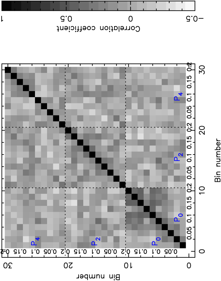
7.4 Redshift-space distortion

We fitted the measured 2dFLenS clustering multipoles using a standard model for the redshift-space galaxy power spectrum as a function of the angle of the Fourier wavevector to the line-of-sight:

$$P_{\rm g}(k,\mu)=b^{2}\,P_{\rm m}(k)\,(1+\beta\mu^{2})^{2}\,\exp{(-k^{2}\mu^{2}\sigma_{v}^{2}/H_{0}^{2})},$$ (69)

where $b$ is the galaxy bias factor, $P_{\rm m}(k)$ is the fiducial non-linear matter power spectrum defined in Section 7.1 and $\beta=f/b$ parameterizes the amplitude of redshift-space distortion in terms of the growth rate of structure $f$. This model combines the large-scale ‘Kaiser limit’ amplitude correction (Kaiser 1987) with a heuristic damping of power on smaller scales that describes a leading-order perturbation theory correction (Scoccimarro 2004) in terms of a free parameter $\sigma_{v}$ with units of km s^-1. Our model is hence characterized by three parameters $(\beta,\sigma_{v},b)$.

We fitted this 3-parameter model to the monopole and quadrupole of both the power spectrum and correlation function in each analysis region. For given values of $(\beta,\sigma_{v},b)$ we deduced the unconvolved model power spectrum multipoles $P_{\ell}(k)$ from $P(k,\mu)$ using Equation 40, which we convolved with the survey window function using Equation 66. The model correlation function multipoles may be determined from $P_{\ell}(k)$ using

$$\xi_{\ell}(s)=\frac{i^{\ell}}{2\pi^{2}}\int dk\,k^{2}\,P_{\ell}(k)\,j_{\ell}(ks),$$ (70)

where $j_{\ell}$ is the spherical Bessel function of order $\ell$. We performed the fits by evaluating the $\chi^{2}$ statistic of each model using the full covariance matrix. For example, for the case of the power spectrum multipoles we determined:

$$\chi^{2}=\sum_{ij}\left[P_{\rm est}(i)-P_{\rm mod}(i)\right]\left[{\rm Cov}^{-1}\right]_{ij}\left[P_{\rm est}(j)-P_{\rm mod}(j)\right]$$ (71)

for each analysis region, and summed the $\chi^{2}$ values. We propagated the errors induced by estimating the inverse of an $N_{\rm bin}\times N_{\rm bin}$ covariance matrix from a limited number of mock catalogues $N_{\rm mock}=65$ by computing the correction determined by Sellentin & Heavens (2016), in which the likelihood of each model is given by

$${\rm Likelihood}\propto\left(1+\frac{\chi^{2}}{N_{\rm mock}-1}\right)^{-N_{\rm mock}/2}.$$ (72)

Our analyses utilized at most $N_{\rm bin}\sim 18$ data points, such that the number of 65 mocks was adequate.

We generated our baseline model fits using the power spectrum multipole measurements in the range $0.02<k<0.2\,h$ Mpc^-1. Our results are not particularly sensitive to the fitting range: Figure 20 demonstrates the low sensitivity of the best-fitting measurement of $\beta$ to the maximum wavenumber used in the fit, with the variation being encompassed by the size of the statistical errors. We prefer to demonstrate the robustness of our results in this manner, rather than by fitting to our mocks, because the mock galaxy catalogues lack a satellite population hence may not be reliable for this purpose.

Figure 20: Dependence of the marginalized measurements of $\beta$ on the maximum wavenumber used when fitting the 2dFLenS power spectrum multipole data. Results are shown for the two redshift ranges $0.15<z<0.43$ (solid black circles) and $0.43<z<0.70$ (open red circles). Measurements for the different redshifts are slightly shifted along the $x$-axis for clarity.

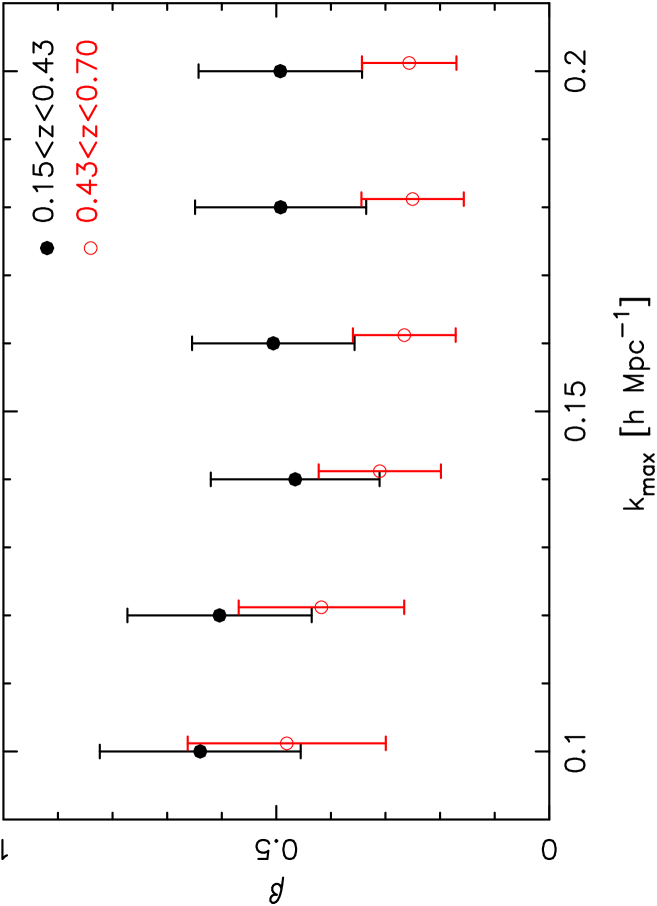
Our marginalized parameter measurements for the $0.15<z<0.43$ datasets are:

$$\beta = 0.49\pm 0.15,$$ (73)

$$\sigma_{v} = 470\pm 110\;{\rm km/s},$$ (74)

$$b = 1.9\pm 0.1.$$ (75)

For $0.43<z<0.7$ we obtain:

$$\beta = 0.26\pm 0.09,$$ (76)

$$\sigma_{v} = 100\pm 100\;{\rm km/s},$$ (77)

$$b = 2.2\pm 0.1.$$ (78)

The best-fitting models are overplotted in Figure 18. The corresponding chi-squared values for the two redshift ranges are $37.1$ and $32.6$, for 33 degrees of freedom, indicating that the models are a good fit to the data, and the best-fitting bias parameters are consistent with those obtained from the projected correlation function in Section 7.1. Figure 21 displays the 2D posterior probability distribution of $(\beta,\sigma_{v})$ for redshift ranges $0.15<z<0.43$ and $0.43<z<0.7$.

Figure 21: Confidence regions of fits for $\beta$ and $\sigma_{v}$, marginalizing over $b$. Results are shown for fits to both correlation function and power spectrum multipoles, for two redshift ranges $0.15<z<0.43$ and $0.43<z<0.70$. $68\%$ and $95\%$ confidence regions are shown in all cases.

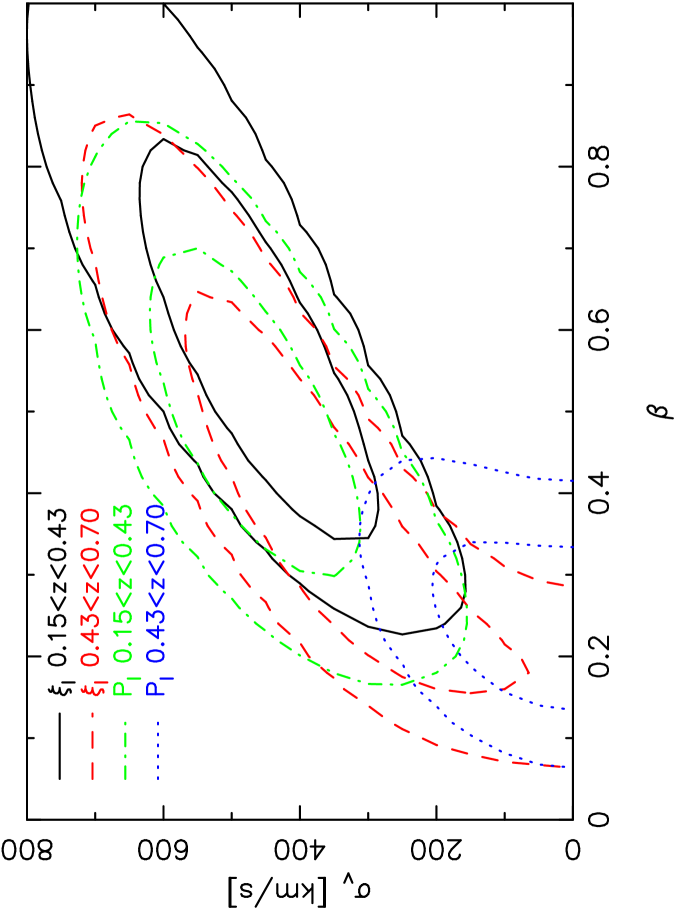
We can compare our $\beta$ measurements to those determined using BOSS LRGs: Sanchez et al. (2014) report $\beta_{\rm LOWZ}=0.38\pm 0.11$ and $\beta_{\rm CMASS}=0.36\pm 0.06$. Our measurements are consistent, albeit with a $\sim 50\%$ larger statistical error. However, the weak lensing data overlapping these 2dFLenS measurements permit some unique applications of our results (Joudaki et al. 2016b, Amon et al. 2016). The amplitudes of our measured redshift-space distortion parameters are also consistent, given their statistical errors, with those predicted by the growth rate in the standard $\Lambda$CDM cosmological model and our best-fitting galaxy bias factors.

As a point of comparison, we also fitted the RSD models to our correlation function multipole measurements in the range $10<s<90\,h^{-1}$ Mpc (again, we note that our results are not particularly sensitive to the fitting range). We overplot the parameter constraints in Figure 21, illustrating that the power spectrum and correlation function multipoles produce consistent results. The best-fitting correlation function multipole models are overplotted in Figures 16.

8 Summary

In this paper we have introduced the 2-degree Field Lensing Survey (2dFLenS), a new galaxy redshift survey performed at the Anglo-Australian Telescope which extends the spectroscopic-redshift coverage of gravitational lensing surveys in the southern sky, with a particular focus on the overlapping Kilo-Degree Survey (KiDS). 2dFLenS contains $70{,}079$ objects with good-quality redshifts, including $40{,}531$ Luminous Red Galaxies and $28{,}269$ objects which form a magnitude-limited nearly-complete sub-sample. The LRGs may be utilized for analysis of galaxy-galaxy lensing, redshift-space distortion and determination of the imaging source redshift distribution by cross-correlation, and the magnitude-limited sample may be employed for direct source classification and photometric-redshift calibration.

In this paper we have presented the survey selection function and clustering measurements for the LRG sample and corresponding mock catalogues. We fitted redshift-space distortion models to the clustering multipoles, finding RSD parameters $\beta=0.49\pm 0.15$ and $0.26\pm 0.09$ for redshift ranges $0.15<z<0.43$ and $0.43<z<0.7$, respectively. These values are consistent with those obtained from LRGs in the Baryon Oscillation Spectroscopic Survey, and (when combined with the best-fitting galaxy bias factors), consistent with the predictions of the standard $\Lambda$CDM cosmological model.

Five associate science papers are currently in preparation:

• Johnson et al. (2016) present a new quadratic-estimation method for constraining the source redshift distribution of an imaging survey via cross-correlations with a spectroscopic redshift survey, with an application to KiDS and 2dFLenS data.

• Joudaki et al. (2016b) perform self-consistent cosmological model fits to overlapping cosmic shear, galaxy-galaxy lensing and redshift-space distortion data from KiDS and 2dFLenS.

• Amon et al. (2016) determine new measurements of the gravitational slip statistic, $E_{G}$, to large scales, using data from KiDS and 2dFLenS.

• Wolf et al. (2016) use the magnitude-limited sample of 2dFLenS redshifts to compare various techniques for direct photometric-redshift calibration based on kernel-density estimation, machine learning with neural networks, and template fits.

• Janssens et al. (2016) analyze the ‘red-nugget’ spare-fibre sample to place new constraints on the redshift evolution of compact early-type galaxies.

2dFLenS data products will be released with the publication of these papers via our website http://2dflens.swin.edu.au.

Appendix A Magnitude transformations

The 2dFLenS LRG selection criteria are inspired by the SDSS, BOSS and eBOSS surveys. Since the filter systems used by the optical imaging surveys used to select 2dFLenS targets – VST OmegaCAM and CFHT MegaCam – are not identical to SDSS filters, we derived magnitude transformations between the different filter systems using an elliptical galaxy template spectrum.

We refer to ATLAS magnitudes as $(u_{A},g_{A},r_{A},i_{A},z_{A})$, CFHT magnitudes as $(u_{C},g_{C},r_{C},i_{C},z_{C})$ or $(u_{C},g_{C},r_{C},y_{C},z_{C})$ (depending on which version of the $i$-band filter was used for a pointing, as described by Erben et al. 2013) and SDSS magnitudes as $(u_{S},g_{S},r_{S},i_{S},z_{S})$. Our template spectrum then yielded transformations

$$\left(\begin{array}[]{c}u_{S}\\ g_{S}\\ r_{S}\\ i_{S}\\ z_{S}\end{array}\right)=\left(\begin{array}[]{ccccc}1.0121&-0.0123&0.0001&0&0\\ 0&1.0091&-0.0103&0.0012&0\\ 0&0&1.1297&-0.1297&0\\ 0&0&0.0308&0.9692&0\\ 0&0&-0.0008&-0.0249&1.0256\end{array}\right)\left(\begin{array}[]{c}u_{A}\\ g_{A}\\ r_{A}\\ i_{A}\\ z_{A}\end{array}\right)$$

$$\left(\begin{array}[]{c}u_{S}\\ g_{S}\\ r_{S}\\ i_{S}\\ z_{S}\end{array}\right)=\left(\begin{array}[]{ccccc}1.2674&-0.3095&0.0442&-0.0021&0\\ 0&1.1574&-0.1651&0.0077&0\\ 0&0&1.0491&-0.0491&0\\ 0&0&0.1057&0.8943&0\\ 0&0&-0.0087&-0.0736&1.0823\end{array}\right)\left(\begin{array}[]{c}u_{C}\\ g_{C}\\ r_{C}\\ i_{C}\\ z_{C}\end{array}\right)$$

$$\left(\begin{array}[]{c}u_{S}\\ g_{S}\\ r_{S}\\ i_{S}\\ z_{S}\end{array}\right)=\left(\begin{array}[]{ccccc}1.2674&-0.3095&0.0443&-0.0022&0\\ 0&1.1574&-0.1656&0.0082&0\\ 0&0&1.0520&-0.0520&0\\ 0&0&0.0520&0.9480&0\\ 0&0&-0.0043&-0.0780&1.0823\end{array}\right)\left(\begin{array}[]{c}u_{C}\\ g_{C}\\ r_{C}\\ y_{C}\\ z_{C}\end{array}\right)$$

The colour coefficients have very little variation with redshift; we use average values in the redshift range $0.15<z<0.7$. Using these transformation matrices we obtained the following relations for the LRG colour variables defined by Equations 3, 4 and 5:

$$c_{\parallel} = 0.7064\,g_{A}+0.5207\,r_{A}-1.2271\,i_{A}-0.216$$ (79)

$$= 0.8102\,g_{C}+0.2821\,r_{C}-1.0923\,i_{C}-0.216$$

$$= 0.8102\,g_{C}+0.3477\,r_{C}-1.1579\,y_{C}-0.216,$$

$$c_{\perp} = -0.2523\,g_{A}+1.3839\,r_{A}-1.1316\,i_{A}-0.18$$ (80)

$$= -0.2894\,g_{C}+1.2469\,r_{C}-0.9576\,i_{C}-0.18$$

$$= -0.2894\,g_{C}+1.3044\,r_{C}-1.0150\,y_{C}-0.18,$$

$$d_{\perp} = -0.1261\,g_{A}+1.2414\,r_{A}-1.1153\,i_{A}$$ (81)

$$= -0.1447\,g_{C}+1.0952\,r_{C}-0.9505\,i_{C}$$

$$= -0.1447\,g_{C}+1.1522\,r_{C}-1.0075\,y_{C}.$$

References

- [1] Ahn, C., et al., 2014, ApJS, 211, 17
- [2] Alam, S., et al., 2016, submitted
- [3] Amon, A., et al., 2016, in preparation
- [4] Anderson, L., et al., 2014, MNRAS, 441, 24
- [5] Aubourg, E., et al., 2015, PhRvD, 92, 3516
- [6] Baldry, I., et al., 2014, MNRAS, 441, 2440
- [7] Becker, M., et al., 2016, PhRvD, 94, 2002
- [8] Bertin, E., Arnouts, S., 1996, AS, 117, 393
- [9] Betoule, M., et al., 2014, A&A, 568, 22
- [10] Beutler, F., et al., 2011, MNRAS, 416, 3017
- [11] Beutler, F., et al., 2012, MNRAS, 423, 3430
- [12] Beutler, F., et al., 2014, MNRAS, 443, 1065
- [13] Bianchi, D., Gil-Marin, H., Ruggeri, R., Percival, W., 2015, MNRAS, 453, 11
- [14] Blake, C., Wall, J., 2002, MNRAS, 337, 993
- [15] Blake, C., et al., 2011a, MNRAS, 415, 2876
- [16] Blake, C., et al., 2011b, MNRAS, 418, 1707
- [17] Blake, C., et al., 2016, MNRAS, 456, 2806
- [18] Bleem, L., et al., 2015, ApJS, 216, 27
- [19] Buddendiek, A., et al., 2016, MNRAS, 456, 3886
- [20] Cai, Y.-C., Bernstein, G., 2012, MNRAS, 422, 1045
- [21] Cannon, R., et al., 2006, MNRAS, 372, 425
- [22] Choi, A., et al., 2016, MNRAS, submitted
- [23] Chow, N., Khoury, J., PhRvD, 80, 4037
- [24] Colless, M., et al., 2001, MNRAS, 328, 1039
- [25] Conley, A., et al., 2011, ApJS, 192, 1
- [26] Cunha, C., Huterer, D., Busha, M., Wechsler, R., 2012, MNRAS, 423, 909
- [27] Damjanov, I., et al., 2009, ApJ, 695, 101
- [28] Damjanov, I., et al., 2015, ApJ, 806, 158
- [29] Dawson, K., et al., 2013, AJ, 145, 10
- [30] Dawson, K., et al., 2016, AJ, 151, 44
- [31] de Jong, J., et al., 2015, A&A, 582, 62
- [32] de la Torre, S., et al., 2013, A&A, 557, 54
- [33] Delubac, T., et al., 2015, A&A, 574, 59
- [34] de Putter, R., Dore, O., Das, S., 2014, ApJ, 780, 185
- [35] de Rham, C., et al., 2008, PhRvL, 100, 1603
- [36] Drinkwater, M., et al., 2010, MNRAS, 401, 1429
- [37] Driver, S., et al., 2011, MNRAS, 413, 971
- [38] Eisenstein, D., et al., 2001, AJ, 122, 2267
- [39] Erben, T., et al., 2005, AN, 326, 432
- [40] Erben, T., et al., 2009, A&A, 493, 1197
- [41] Erben, T., et al., 2013, MNRAS, 433, 2545
- [42] Eriksen, M., Gaztanaga, E., 2015, MNRAS, 451, 1553
- [43] Feldman, H., Kaiser, N., Peacock, J., 1994, ApJ, 426, 23
- [44] Fixsen, D., Cheng, E., Gales, J., Mather, J., Shafer, R., Wright, E., 1996, ApJ, 473, 576
- [45] Font-Ribera, A., McDonald, P., Mostek, N., Reid, B., Seo, H.-J., Slosar, A., 2014, JCAP, 5, 23
- [46] Gaztanaga, E., Eriksen, M., Crocce, M., Castander, F., Fosalba, P., Marti, P., Miquel, R., Cabre, A., 2012, MNRAS, 422, 2904
- [47] Gilbank, D., Gladders, M., Yee, H., Hsieh, B., 2011, AJ, 141, 94
- [48] Guo, H., et al., 2014, MNRAS, 441, 2398
- [49] Gwyn, S., 2012, AJ, 143, 38
- [50] Harnois-Deraps, J., Pen, U.-L., Iliev, I., Merz, H., Emberson, J., Desjacques, V., 2013, MNRAS, 436, 540
- [51] Harnois-Deraps, J., van Waerbeke, L., 2015, MNRAS, 450, 2857
- [52] Heymans, C., et al., 2012, MNRAS, 427, 146
- [53] Hildebrandt, H., et al., 2012, MNRAS, 421, 2355
- [54] Hildebrandt, H., et al., 2016a, MNRAS, submitted
- [55] Hildebrandt, H., et al., 2016b, MNRAS, submitted
- [56] Hinton, S., Davis, T., Lidman, C., Glazebrook, K., Lewis, G., 2016, Astronomy & Computing, 15, 61
- [57] Huff, E., Eifler, T., Hirata, C., Mandelbaum, R., Schlegel, D., Seljack, U., 2014, MNRAS, 440, 1322
- [58] Janssens, S., et al., 2016, in preparation
- [59] Johnson, A., et al., 2016, in preparation
- [60] Joudaki, S., et al., 2016a, submitted
- [61] Joudaki, S., et al., 2016b, in preparation
- [62] Kaiser, N., 1987, MNRAS, 227, 1
- [63] Kaiser, N., Squires, G., Broadhurst, T., 1995, ApJ, 449, 460
- [64] Kazin, E., et al., 2014, MNRAS, 441, 3524
- [65] Kirk, D., Lahav, O., Bridle, S., Jouvel, S., Abdalla, F., Frieman, J., 2015, MNRAS, 451, 4424
- [66] Kuijken, K., et al., 2015, MNRAS, 454, 3500
- [67] Landy S., Szalay A., 1993, ApJ, 412, 64
- [68] Lewis, A., Challinor, A., Lasenby, A., 2000, ApJ, 538, 473
- [69] Lewis, I., et al., 2002, MNRAS, 333, 279
- [70] Lidman, C., et al., 2016, in preparation
- [71] Ma, Z., Hu, W., Huterer, D., 2006, ApJ, 636, 21
- [72] Mandelbaum, R., et al., 2013, MNRAS, 432, 1544
- [73] Marin, F., Beutler, F., Blake, C., Koda, J., Kazin, E., Schneider, D., 2016, MNRAS, 455, 4046
- [74] McDonald, P., Seljak, U., 2009, JCAP, 10, 7
- [75] McQuinn, M., White, M., 2013, MNRAS, 433, 2857
- [76] Mehrtens, N., et al., 2012, MNRAS, 423, 1024
- [77] Miszalski, B., et al., 2006, MNRAS, 371, 1537
- [78] More, S., Miyatake, H., Mandelbaum, R., Takada, M., Spergel, D., Brownstein, J., Schneider, D., 2015, ApJ, 806, 2
- [79] Newman, J., et al., 2015, APh, 63, 81
- [80] Pickles, A., 1998, PASP, 110, 863
- [81] Planck collaboration (2015 results XIII), submitted
- [82] Poggianti, B., et al., 2013, ApJ, 762, 77
- [83] Prakash, A., Licquia, T., Newman, J., Rao, S., 2015, ApJ, 803, 105
- [84] Reyes, R., et al., 2010, Nature, 464, 256
- [85] Samushia, L., et al., 2014, MNRAS, 439, 3504
- [86] Sanchez, A., et al., 2014, MNRAS, 440, 2692
- [87] Saunders, W., et al., 2004, SPIE, 5492, 389
- [88] Saunders, W., Cannon, R., Sutherland, W., 2004, Anglo-Australian Observatory Newsletter, 106, 16
- [89] Schirmer, M., 2013, ApJS, 209, 21
- [90] Schlegel, D., Finkbeiner, D., Davis, M., 1998, ApJ, 500, 525
- [91] Scoccimarro, R., 2004, PhRvD, 70, 83007
- [92] Scoccimarro, R., 2015, PhRvD, 92, 3532
- [93] Sellentin, E., Heavens, A., 2016, MNRAS, 456, 132
- [94] Shanks, T., et al., 2015, MNRAS, 451, 4238
- [95] Sharp et al., 2006, SPIE, 6269, 14
- [96] Simpson, F., et al., 2013, MNRAS, 429, 2249
- [97] Skrutskie, M., et al., 2006, AJ, 131, 1163
- [98] Song, Y.-S., et al., 2011, PhRvD, 84, 3523
- [99] Sotiriou, T., Faraoni, V., 2010, RvMP, 82, 451
- [100] Suzuki, N., et al., 2012, ApJ, 746, 85
- [101] Takahashi, R., Sato, M., Nishimichi, T., Taruya, A., Oguri, M., 2012, ApJ, 761, 152
- [102] Taylor, E., et al., 2010, ApJ, 720, 723
- [103] Tonry, J., Davis, M., 1979, AJ, 84, 1511
- [104] Valentinuzzi, T., et al., 2010, ApJ, 712, 226
- [105] van Dokkum, P., et al., 2008, ApJ, 677, 5
- [106] Wolf, C., et al., 2016, in preparation
- [107] Yamamoto, K., Nakamichi, M., Kamino, A., Bassett, B., Nishioka, H., 2006, PASJ, 58, 93
- [108] Yanny, B., et al., 2009, ApJ, 700, 1282
- [109] Yuan, F., et al., 2015, MNRAS, 452, 3047
- [110] Zacharias, N., Finch, C., Girard, T., Henden, A., Bartlett, J., Monet, D., Zacharias, M., 2013, AJ, 145, 44
- [111] Zhang, P., et al., 2007, PhRvL, 99, 1302