Laser-induced torques in metallic ferromagnets

Abstract

We study laser-induced torques in bcc Fe, hcp Co and $L1_{0}$ FePt based on first-principles electronic structure calculations and the Keldysh nonequilibrium formalism. We find that the torques have two contributions, one from the inverse Faraday effect (IFE) and one from the optical spin-transfer torque (OSTT). Depending on the ferromagnet at hand and on the quasiparticle broadening the two contributions may be of similar magnitude or one contribution may dominate over the other. Additionally, we determine the nonequilibrium spin polarization in order to investigate its relation to the torque. We find the torques and the perpendicular component of the nonequilibrium spin polarization to be odd in the helicity of the laser light, while the spin polarization that is induced parallel to the magnetization is helicity-independent. The parallel component of the nonequilibrium spin polarization is orders of magnitude larger than the perpendicular component. In the case of hcp Co we find good agreement between the calculated laser-induced torque and a recent experiment.

I Introduction

Several mechanisms induce torques on the magnetization in magnetically ordered materials when laser pulses are applied Kirilyuk et al. (2010). When circularly polarized light is used, an effective magnetic field parallel to the light wave vector acts on the magnetization due to the inverse Faraday effect (IFE) Kimel et al. (2005) (Figure 1a). The IFE is thought to play a crucial role in the laser-induced magnetization reversal in ferromagnetic thin films Lambert et al. (2014); John et al. (2016). Additionally, there is a light-induced effective magnetic field perpendicular to both the magnetization and the light wave vector, which leads to the optical spin transfer torque (OSTT) Nemec et al. (2012) (Figure 1b). Besides these non-thermal effects, the laser-induced heating can also generate torques due to heat-induced modifications of the magnetic anisotropy fields van Kampen et al. (2002). Furthermore, laser pulses excite superdiffusive spin currents in magnetic heterostructures Battiato et al. (2010); Malinowski et al. (2008); Melnikov et al. (2011); Seifert et al. (2016), which mediate spin-transfer torques when they flow from one magnetic layer into another Schellekens et al. (2014). Finally, the laser-induced heating drives spin-currents due to the spin-dependent Seebeck effect, which leads to thermal spin transfer torques in metallic spin-valves Choi et al. (2015).

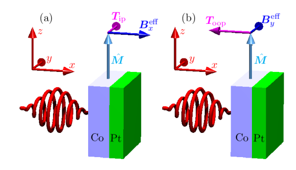
Figure 1: A circularly polarized light pulse propagates in $x$ direction and hits a Co/Pt bilayer. The magnetization direction $\hat{{\bm{M}}}$ is along the $z$ axis. The laser-induced torque ${\bm{T}}$ has two components: (a) The in-plane component ${\bm{T}}_{\rm ip}$ can be attributed to an effective magnetic field ${\bm{B}}^{\rm eff}_{x}$ in $x$ direction. ${\bm{T}}_{\rm ip}$ leads to an initial in-plane tilt of $\hat{{\bm{M}}}$. (b) The out-of-plane component ${\bm{T}}_{\rm oop}$ can be attributed to the $y$ component ${\bm{B}}^{\rm eff}_{y}$ of a laser-induced effective magnetic field and leads to an initial out-of-plane tilt of $\hat{{\bm{M}}}$.

In the following we will consider only the effective magnetic fields, torques and non-equilibrium spin-densities related to the IFE and OSTT. In ferromagnets the light-induced non-equilibrium spin-density can generally exhibit a component parallel to the equilibrium magnetization as well as a perpendicular one. The perpendicular component exerts a torque on the magnetization and tilts it. This laser-induced torque has been investigated in metallic ferromagnets in recent experiments Choi (2015); Huisman et al. (2016): In Co a 50 fs laser pulse with fluence 1 mJ cm^-2 induces an effective magnetic field whose perpendicular component has been estimated at 0.2 Tesla. One experiment Choi (2015) was interpreted in terms of an initial out-of-plane tilting of the magnetization due to an out-of-plane torque (Figure 1b), while the second experiment Huisman et al. (2016) was interpreted in terms of an initial in-plane tilting due to an in-plane torque (see Figure 1a). The out-of-plane tilting has been ascribed to the OSTT and an in-plane tilting is expected from the IFE. Both experiments find that the magnetization is only tilted when circularly polarized light is used and that the effect changes sign when the helicity of the light is reversed. In both experiments the Co layer is sufficiently thick (10nm) to assume that the laser-induced effective magnetic fields responsible for the magnetization tilting can be modelled theoretically based on the bulk electronic structure of Co, neglecting the Co/Pt interface. In one experiment Choi (2015) the Pt capping layer mainly serves to prevent oxidation of the Co layer. In the second experiment Huisman et al. (2016) the inverse spin-orbit torque (ISOT) Freimuth et al. (2015) due to the structural inversion asymmetry at the Co/Pt interface is exploited to convert the magnetization tilting into an interfacial photocurrent.

On the theory side, for the special case of light-propagation direction parallel to the magnetization, light-induced effective magnetic fields parallel to the magnetization have been studied in transition metal ferromagnets Berritta et al. (2016) with ab-initio methods as well as in the ferromagnetic Rashba model Qaiumzadeh and Titov (2016). Both theoretical works find that not only circularly polarized light but also linearly polarized light induces effective magnetic fields parallel to the magnetization. Moreover, it was found that the light-induced spin polarization parallel to the magnetization is almost helicity-independent in Fe, Co, and Ni Berritta et al. (2016). Since in contrast the light-induced torques observed experimentally are odd in the helicity Huisman et al. (2016) is seems that effective magnetic fields perpendicular to the magnetization direction depend differently on the light helicity than the parallel component in these metallic ferromagnets.

In this work we use ab-initio density functional theory in order to study all components of the light-induced non-equilibrium spin density and of the resulting torques and effective magnetic fields in Fe, Co and FePt. This allows us to answer the two questions raised above: (i) Is the laser-induced torque on the magnetization in Figure 1 pointing in the in-plane or in the out-of-plane direction? (ii) How do the parallel and perpendicular components of the light-induced effective magnetic field differ regarding their size and their dependence on the light polarization?

This paper is structured as follows: In section II we describe our computational approach, which uses the Keldysh non-equilibrium formalism to obtain the response in second order to the electric field of the laser. Details of the derivation and of the numerical implementation are given in appendix A and in appendix B, respectively. Before presenting our results in section III we first describe the computational parameters used in the calculations in III.1. In section III.2 we discuss the effective magnetic fields that give rise to the laser-induced torques and in section III.3 we investigate the laser-induced nonequilibrium spin density. We conclude with a summary in section IV.

II Computational method

We use Kohn-Sham density functional theory to describe interacting many-electron systems by the effective single-particle Hamiltonian

$$H({\bm{r}})=H_{0}({\bm{r}})-{\bm{m}}\cdot\hat{{\bm{M}}}\Omega^{\rm xc}({\bm{r}}),$$ (1)

where $H_{0}$ contains kinetic energy, scalar potential and spin-orbit interaction (SOI), ${\bm{m}}=-\mu_{\rm B}{\bm{\sigma}}$ is the spin magnetic moment operator, $\mu_{\rm B}$ is the Bohr magneton, ${\bm{\sigma}}=(\sigma_{x},\sigma_{y},\sigma_{z})^{\rm T}$ is the vector of Pauli spin matrices, $\hat{{\bm{M}}}$ is a normalized vector parallel to the magnetization, $\Omega^{\rm xc}({\bm{r}})=\frac{1}{2\mu_{\rm B}}[V^{\rm eff}_{\rm minority}({\bm{r}})-V^{\rm eff}_{\rm majority}({\bm{r}})]$ is the exchange field, and $V^{\rm eff}_{\rm minority}({\bm{r}})$ and $V^{\rm eff}_{\rm majority}({\bm{r}})$ are the effective potentials of minority and majority electrons, respectively.

The interaction with the laser field is described by the perturbation to the Hamiltonian

$$\delta H(t)=e{\bm{v}}\cdot{\bm{A}}(t),$$ (2)

where $e$ is the elementary positive charge, ${\bm{v}}$ is the velocity operator and

$${\bm{A}}(t)={\rm Re}\left[\frac{E_{0}\bm{\epsilon}e^{-i\omega t}}{i\omega}\right]$$ (3)

is the vector potential. The corresponding electric field of the laser is

$${\bm{E}}(t)=-\frac{\partial{\bm{A}}(t)}{\partial t}={\rm Re}\left[E_{0}\bm{\epsilon}e^{-i\omega t}\right],$$ (4)

where $\bm{\epsilon}$ is the light-polarization vector and $E_{0}$ is the amplitude of the electric field. We assume that $E_{0}$ is real-valued. However, $\bm{\epsilon}$ may be complex. For example, to describe left-circularly and right-circularly polarized light propagating in $x$ direction we use $\bm{\epsilon}=(0,1,i)/\sqrt{2}$ and $\bm{\epsilon}=(0,1,-i)/\sqrt{2}$, respectively.

The laser-induced change of spin polarization is given by Qaiumzadeh and Titov (2016); Misawa et al. (2011); Taguchi and Tatara (2011); Taguchi et al. (2012)

$$\delta{\bm{S}}=\int{\rm d}^{3}r\,\delta{\bm{s}}({\bm{r}})=\frac{\hbar}{2i}{\rm Tr}\left[{\bm{\sigma}}G^{<}\right],$$ (5)

where $G^{<}$ is the lesser Green function. $\delta{\bm{S}}$ is the integral of the nonequilibrium spin-density $\delta{\bm{s}}({\bm{r}})$ over the simulation volume, i.e., the change of the total electron spin in the simulation volume, when $\hat{{\bm{M}}}$ in Eq. (1) is kept fixed. The torque on the magnetization due to the nonequilibrium spin-density is given by Haney et al. (2007, 2008); Freimuth et al. (2015, 2014)

$${\bm{T}}=\frac{2\mu_{\rm B}}{\hbar}\int{\rm d}^{3}r\,\Omega^{\rm xc}({\bm{r}})\delta{\bm{s}}({\bm{r}})\times\hat{{\bm{M}}}.$$ (6)

Since the nonequilibrium spin-density $\delta{\bm{s}}({\bm{r}})$ as well as the exchange field $\Omega^{\rm xc}({\bm{r}})$ vary strongly on the atomic scale, it is generally not possible to calculate ${\bm{T}}$ exactly from $\delta{\bm{S}}$. Therefore, we calculate the torque from

$${\bm{T}}=i{\rm Tr}\left[{\bm{\mathcal{T}}}G^{<}\right],$$ (7)

where ${\bm{\mathcal{T}}}({\bm{r}})={\bm{m}}\times\hat{{\bm{M}}}\Omega^{\rm xc}({\bm{r}})$ is the torque operator Freimuth et al. (2015, 2014); Haney et al. (2013); Turek et al. (2015); Wimmer et al. (2016). It is clear that the laser-induced nonequilibrium magnetization in paramagnets and diamagnets consists of both spin and orbital contributions. Consequently, a recent ab-initio study on the IFE considered both spin and orbital parts of the laser-induced nonequilibrium magnetization Berritta et al. (2016). However, in the present work we are mostly interested in the laser-induced torques on the magnetization in ferromagnets, which are determined by the nonequilibrium spin-density according to Eq. (6). While the laser-induced orbital polarization corresponds to orbital currents, which lead to magnetic fields according to the Maxwell equations, the resulting torques are negligible in comparison to the torques described by Eq. (6). We therefore do not consider the laser-induced orbital polarization in this work.

In systems with broken inversion symmetry, ${\bm{T}}$ contains a contribution that is first order in ${\bm{E}}(t)$, the so-called spin-orbit torque (SOT) Freimuth et al. (2015, 2014); Haney et al. (2013); Wimmer et al. (2016); Garello et al. (2013); Ciccarelli et al. (2016). However, this first-order contribution oscillates with frequency $\omega$. Since the light frequency $\omega$ is much higher than the ferromagnetic resonance frequency, this oscillating contribution will not induce significant magnetization dynamics. Therefore, we consider the dc part in the response to a continuous laser field. The contribution to ${\bm{T}}$ that is second order in ${\bm{E}}(t)$ contains such static terms. They can arise for example from the time-independent part $E_{0}^{2}{\rm Re}[\epsilon_{i}\epsilon_{j}^{*}]/2$ in

$$E_{i}(t)E_{j}(t)\!=\!\frac{E_{0}^{2}}{4}\!\left[\epsilon_{i}\epsilon^{*}_{j}\!+\!\epsilon^{*}_{i}\epsilon_{j}\!+\!\epsilon_{i}\epsilon_{j}e^{-2i\omega t}\!+\!\epsilon^{*}_{i}\epsilon^{*}_{j}e^{2i\omega t}\right].$$ (8)

The dc correction of $G^{<}$ proportional to $E_{0}^{2}$ can be conveniently derived within the Keldysh nonequilibrium formalism. Details of the derivation are given in Appendix A. The resulting torque is given by the expression

$$T_{i}=\frac{a_{0}^{3}I}{c}\left(\frac{\mathcal{E}_{\rm H}}{\hbar\omega}\right)^{2}{\rm Im}\sum_{jk}\epsilon_{j}\epsilon_{k}^{*}\chi_{ijk},$$ (9)

where $c$ is the velocity of light, $a_{0}=4\pi\epsilon_{0}\hbar^{2}/(me^{2})$ is Bohr’s radius, $I=\epsilon_{0}cE_{0}^{2}/2$ is the intensity of light, $\epsilon_{0}$ is the vacuum permittivity and $\mathcal{E}_{\rm H}=e^{2}/(4\pi\epsilon_{0}a_{0})$ is the Hartree energy. The tensor $\chi_{ijk}$ is given by

$$\chi_{ijk}= \frac{2}{\mathcal{N}\hbar a_{0}^{2}\mathcal{E}_{\rm H}}\sum_{{\bm{k}}}\int{\rm d}\mathcal{E}{\rm Tr}\Big{[}$$ (10)

$$f(\mathcal{E})\mathcal{T}_{i}G^{\rm R}_{{\bm{k}}}(\mathcal{E})v_{j}G^{\rm R}_{{\bm{k}}}(\mathcal{E}-\hbar\omega)v_{k}G^{\rm R}_{{\bm{k}}}(\mathcal{E})$$

$$- f(\mathcal{E})\mathcal{T}_{i}G^{R}_{{\bm{k}}}(\mathcal{E})v_{j}G^{R}_{{\bm{k}}}(\mathcal{E}-\hbar\omega)v_{k}G^{A}_{{\bm{k}}}(\mathcal{E})$$

$$+ f(\mathcal{E})\mathcal{T}_{i}G^{\rm R}_{{\bm{k}}}(\mathcal{E})v_{k}G^{\rm R}_{{\bm{k}}}(\mathcal{E}+\hbar\omega)v_{j}G^{\rm R}_{{\bm{k}}}(\mathcal{E})$$

$$- f(\mathcal{E})\mathcal{T}_{i}G^{\rm R}_{{\bm{k}}}(\mathcal{E})v_{k}G^{\rm R}_{{\bm{k}}}(\mathcal{E}+\hbar\omega)v_{j}G^{\rm A}_{{\bm{k}}}(\mathcal{E})$$

$$+ f(\mathcal{E}-\hbar\omega)\mathcal{T}_{i}G^{R}_{{\bm{k}}}(\mathcal{E})v_{j}G^{R}_{{\bm{k}}}(\mathcal{E}-\hbar\omega)v_{k}G^{A}_{{\bm{k}}}(\mathcal{E})$$

$$+ f(\mathcal{E}+\hbar\omega)\mathcal{T}_{i}G^{\rm R}_{{\bm{k}}}(\mathcal{E})v_{k}G^{\rm R}_{{\bm{k}}}(\mathcal{E}+\hbar\omega)v_{j}G^{\rm A}_{{\bm{k}}}(\mathcal{E})\Big{]},$$

where $\mathcal{N}$ is the number of ${\bm{k}}$ points used to sample the Brillouin zone, $f(\mathcal{E})$ is the Fermi distribution function, $G^{\rm R}_{{\bm{k}}}(\mathcal{E})$ is the retarded Green function and $G^{\rm A}_{{\bm{k}}}(\mathcal{E})=[G^{\rm R}_{{\bm{k}}}(\mathcal{E})]^{\dagger}$ is the advanced Green function. In order to simulate disorder and finite lifetimes of the electronic states we use the constant broadening $\Gamma$. Therefore, the energy dependence of the Green function is known analytically:

$$G^{\rm R}_{{\bm{k}}}(\mathcal{E})=\hbar\sum_{n}\frac{|{\bm{k}}n\rangle\langle{\bm{k}}n|}{\mathcal{E}-\mathcal{E}_{{\bm{k}}n}+i\Gamma},$$ (11)

where $|{\bm{k}}n\rangle$ and $\mathcal{E}_{{\bm{k}}n}$ are eigenstates and eigenenergies, respectively, of the Hamiltonian in Eq. (1), i.e.,

$$H|{\bm{k}}n\rangle=\mathcal{E}_{{\bm{k}}n}|{\bm{k}}n\rangle.$$ (12)

This simple form of $G^{\rm R}_{{\bm{k}}}(\mathcal{E})$ allows us to perform the energy integrations in Eq. (10) analytically. The resulting expressions are given in Appendix B for the case of zero temperature.

It is convenient to discuss the laser-induced torque ${\bm{T}}$ in terms of the equivalent effective magnetic field ${\bm{B}}^{\rm eff}$ that one needs to apply in order to produce the same torque on the magnetization. It is given by

$${\bm{B}}^{\rm eff}=\frac{{\bm{T}}\times\hat{{\bm{M}}}}{\mu},$$ (13)

where $\mu$ is the magnetic moment in the simulation volume.

The expressions that we use to evaluate the non-equilibrium spin density $\delta{\bm{S}}$, Eq. (5), are similar to Eq. (9) and Eq. (10):

$$\delta S_{i}=-\frac{\hbar}{2}\frac{a_{0}^{3}I}{c}\frac{\mathcal{E}_{\rm H}}{\left(\hbar\omega\right)^{2}}{\rm Im}\sum_{jk}\epsilon_{j}\epsilon_{k}^{*}\bar{\chi}_{ijk},$$ (14)

where

$$\bar{\chi}_{ijk}= \frac{2}{\mathcal{N}\hbar a_{0}^{2}}\sum_{{\bm{k}}}\int{\rm d}\mathcal{E}{\rm Tr}\Big{[}$$ (15)

$$f(\mathcal{E})\sigma_{i}G^{\rm R}_{{\bm{k}}}(\mathcal{E})v_{j}G^{\rm R}_{{\bm{k}}}(\mathcal{E}-\hbar\omega)v_{k}G^{\rm R}_{{\bm{k}}}(\mathcal{E})$$

$$- f(\mathcal{E})\sigma_{i}G^{R}_{{\bm{k}}}(\mathcal{E})v_{j}G^{R}_{{\bm{k}}}(\mathcal{E}-\hbar\omega)v_{k}G^{A}_{{\bm{k}}}(\mathcal{E})$$

$$+ f(\mathcal{E})\sigma_{i}G^{\rm R}_{{\bm{k}}}(\mathcal{E})v_{k}G^{\rm R}_{{\bm{k}}}(\mathcal{E}+\hbar\omega)v_{j}G^{\rm R}_{{\bm{k}}}(\mathcal{E})$$

$$- f(\mathcal{E})\sigma_{i}G^{\rm R}_{{\bm{k}}}(\mathcal{E})v_{k}G^{\rm R}_{{\bm{k}}}(\mathcal{E}+\hbar\omega)v_{j}G^{\rm A}_{{\bm{k}}}(\mathcal{E})$$

$$+ f(\mathcal{E}-\hbar\omega)\sigma_{i}G^{R}_{{\bm{k}}}(\mathcal{E})v_{j}G^{R}_{{\bm{k}}}(\mathcal{E}-\hbar\omega)v_{k}G^{A}_{{\bm{k}}}(\mathcal{E})$$

$$+ f(\mathcal{E}+\hbar\omega)\sigma_{i}G^{\rm R}_{{\bm{k}}}(\mathcal{E})v_{k}G^{\rm R}_{{\bm{k}}}(\mathcal{E}+\hbar\omega)v_{j}G^{\rm A}_{{\bm{k}}}(\mathcal{E})\Big{]}.$$

III Results

III.1 Computational details

We employ the full-potential linearized augmented-plane-wave (FLAPW) program FLEUR fle in order to determine the electronic structure of bcc Fe, $L1_{0}$ FePt and hcp Co selfconsistently within the generalized-gradient approximation Perdew et al. (1996) to density-functional theory. The experimental lattice constants are used. In the case of Fe and FePt the crystallographic $c$ and $a$ axes are aligned with the $z$ and $y$ directions, respectively (Figure 1 illustrates the coordinate frame). In the case of Co we performed two calculations in order to assess the anisotropy of the laser-induced torques: One calculation where the $c$ axis is aligned with the $z$ direction, and one where the $c$ axis is aligned with the $x$ direction (in both calculations the $a$ axis is in $y$ direction).

In order to perform the Brillouin zone integrations in Eq. (10) and in Eq. (15) computationally efficiently based on the Wannier interpolation technique Marzari et al. (2012), we constructed 18 maximally localized Wannier functions (MLWFs) per transition metal atom from an $8\times 8\times 8$ ${\bm{k}}$ mesh Mostofi et al. (2008); Freimuth et al. (2008). In order to describe room temperature experiments in Fe, FePt and Co, it is a very good approximation to set the temperature in the Fermi distribution function $f(\mathcal{E})$ in Eq. (10) and in Eq. (15) to zero. Effects of room-temperature phonon-scattering can be modelled by the phenomenological broadening parameter $\Gamma$ in Eq. (11). The energy integrations in Eq. (10) and in Eq. (15) are performed analytically, as described in Appendix B. We vary $\Gamma$ in the range from 5 meV to 0.4 eV. For this range of broadening $\Gamma$ we find that not more than $256\times 256\times 256$ ${\bm{k}}$ points are needed in order to converge the Brillouin zone sampling in Eq. (10) and Eq. (15).

In section III.2 and III.3 we discuss laser induced torques and spin polarization for the laser intensity $I=10$ GW/cm². The photon energy is set to 1.55 eV. The light is propagating into the $x$ direction (as illustrated in Figure 1) and the polarization vector is $\bm{\epsilon}_{\lambda}=(0,1,i\lambda)/\sqrt{2}$, where $\lambda=+1$ and $\lambda=-1$ describe left and right circularly polarized light, respectively. The magnetization is set along the $z$ direction.

III.2 Laser-induced torques

We discuss the laser-induced torques in terms of the equivalent effective magnetic fields defined in Eq. (13). Figure 2 shows these laser-induced effective magnetic fields in Fe, Co and FePt. In the case of Co we show results of two different calculations: One where the crystallographic $c$ axis is in $z$ direction ($c\|z$) and one where it is in $x$ direction ($c\|x$). The effective field in $x$ direction, $B^{\rm eff}_{x}$, arises due to the IFE in this case. The effective field in $y$ direction arises due to the OSTT. Both $B^{\rm eff}_{x}$ and $B^{\rm eff}_{y}$ are odd in the helicity $\lambda$. In the geometry of Figure 1 $B^{\rm eff}_{x}$ leads to an in-plane torque and thus an initial in-plane tilting of the magnetization, while $B^{\rm eff}_{y}$ leads to an out-of-plane torque and thus an initial out-of-plane tilting. The effective fields depend strongly on the broadening $\Gamma$, which varies between 5 meV and 0.4 eV in the figure. In Fe $B^{\rm eff}_{y}$ is always larger than $B^{\rm eff}_{x}$ in the considered $\Gamma$-range, while in FePt $B^{\rm eff}_{x}$ is always larger than $B^{\rm eff}_{y}$. In Co $B^{\rm eff}_{x}$ dominates over $B^{\rm eff}_{y}$ for small and medium $\Gamma$, while for very large broadening $B^{\rm eff}_{y}$ becomes larger than $B^{\rm eff}_{x}$. In Co the component $B^{\rm eff}_{x}$ exhibits a strong anisotropy at small $\Gamma$.

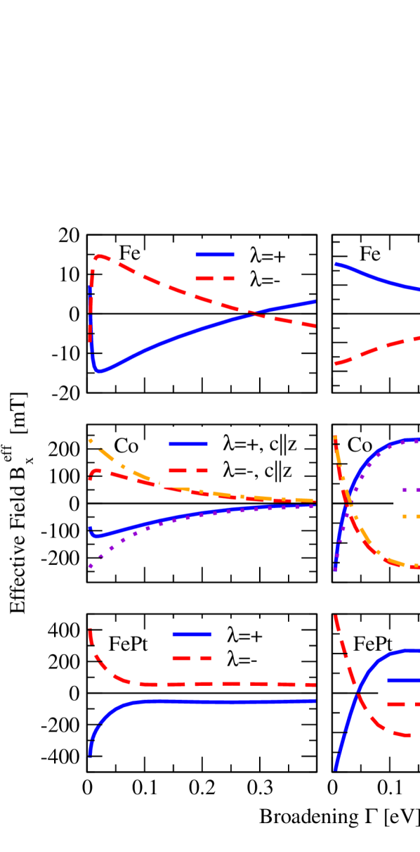
Figure 2: Laser-induced effective magnetic fields $B^{\rm eff}_{x}$ (left column) and $B^{\rm eff}_{y}$ (right column) in Fe, Co and FePt as a function of broadening $\Gamma$ at $I=10$ GW/cm². $\hat{{\bm{M}}}$ is in $z$ direction. $\lambda=+$ and $\lambda=-$ denote left and right circularly polarized light, respectively. In the case of Co, results are shown for $c$ axis in $z$ direction ($c\|z$) and $c$ axis in $x$ direction ($c\|x$).

In previous works we used $\Gamma$ = 25 meV to model room-temperature experiments on Co/Pt bilayers Freimuth et al. (2014). At $\Gamma$ = 25 meV we find $B^{\rm eff}_{x}=118$ mT and $B^{\rm eff}_{y}=0.23$ mT in Co for the $c\|z$ case. For $c\|x$ we find $B^{\rm eff}_{x}=194$ mT and $B^{\rm eff}_{y}=3.1$ mT in Co. Similarly large anisotropies have been predicted for the anomalous Hall effect in Co Roman et al. (2009). At $\Gamma$ = 25 meV the component $B^{\rm eff}_{x}$ strongly dominates over $B^{\rm eff}_{y}$, leading to an initial in-plane tilt of the magnetization in the geometry of figure 1, consistent with the experimental interpretation Huisman et al. (2016). For a 50 fs laser-pulse with a fluence of 1 mJ/cm² Huisman et al. (2016), which corresponds to an intensity of the order of $I\approx 1~{}$mJcm${}^{-2}/(50$ fs)= 20 GWcm^-2, an effective field of 200 mT in Co was estimated from experiments Huisman et al. (2016), corresponding to roughly $100$ mT at $I$= 10 GWcm^-2. The experimental geometry corresponds to the $c\|x$ case in our simulation. Our theoretical result of $B^{\rm eff}_{x}=194$ mT is thus larger than the experimental estimate by roughly a factor of 2. One potential reason for the discrepancy is that laser-pulses were used in the experiment, while our simulation assumes a continuous laser beam. Additionally, the effective magnetic field is strongly $\Gamma$ dependent according to our calculation and any disorder present in the 10 nm Co film used in the experiment might correspond to a value of $\Gamma$ larger than 25 meV, which we assumed in this comparison.

At $\Gamma$ = 25 meV $B^{\rm eff}_{x}$ strongly dominates over $B^{\rm eff}_{y}$ in Co and FePt. On the other hand, the case of Fe shows that generally $B^{\rm eff}_{x}$ and $B^{\rm eff}_{y}$ can be of similar magnitude in transition metal ferromagnets. If an Fe layer is used instead of the Co layer in Figure 1, the initial magnetization tilt will be a mixture of in-plane and out-of-plane according to our calculations. While the helicity-dependent component of the photocurrent in Co/Pt bilayers arises from an initial in-plane tilting Huisman et al. (2016) combined with the odd component of the ISOT, also out-of-plane tilting gives rise to photocurrents via the even ISOT component Freimuth et al. (2015). The photocurrent density ${\bm{J}}$ induced by the initial magnetization tilt in the bilayer geometry of figure 1 can be written as Huisman et al. (2016)

$${\bm{J}}= -\frac{\gamma t^{\rm odd}}{V}\hat{{\bm{e}}}_{x}\times\left[\hat{{\bm{M}}}\times{\bm{B}}^{\rm eff}\right]$$ (16)

$$-\frac{\gamma t^{\rm even}}{V}\hat{{\bm{e}}}_{x}\times\left[\hat{{\bm{M}}}\times\left(\hat{{\bm{M}}}\times{\bm{B}}^{\rm eff}\right)\right],$$

where $\gamma$ is the electron gyromagnetic factor, $V$ is the volume, $\hat{{\bm{e}}}_{x}$ is a unit vector along the $x$ axis and the coefficients $t^{\rm odd}$ and $t^{\rm even}$ characterize the odd and even component of the SOT, respectively. When ${\bm{B}}^{\rm eff}$ points in $x$ direction, the photocurrent is proportional to $t^{\rm odd}$ and when ${\bm{B}}^{\rm eff}$ points in $y$ direction, the photocurrent is proportional to $t^{\rm even}$. In both cases the photocurrent is flowing along the magnetization direction. Therefore, we expect that the helicity-dependent component of the photocurrent in experiments analogous to the ones in Ref. Huisman et al. (2016) but based on Fe/Pt bilayers contains contributions from both the even and odd ISOT. The differences in the effective fields ${\bm{B}}^{\rm eff}$ between Fe, Co and FePt suggest that ferromagnetic materials can be designed such that the IFE is zero and the OSTT is nonzero. Using such materials in experiments analogous to the ones in Ref. Huisman et al. (2016) would allow the contactless measurement of the even ISOT, which contains information about the spin Hall effect, from the helicity-odd component of the photocurrent. In fact, the helicity-even component of the photocurrent is already used for contactless measurement of the spin Hall effect Seifert et al. (2016).

In order to investigate the dependence of $B^{\rm eff}_{x}$ and $B^{\rm eff}_{y}$ on SOI, we linearly scale the spin-orbit interaction in the Hamiltonian with a factor $\xi$ such that SOI is switched off for $\xi$=0 and that the full SOI is active for $\xi$=1. Figure 3 shows the laser-induced effective magnetic fields in Fe as a function of $\xi$. When SOI is switched off $B^{\rm eff}_{x}$ and $B^{\rm eff}_{y}$ vanish, which proves that SOI is the origin of these laser-induced effective magnetic fields.

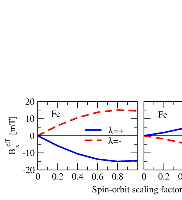
Figure 3: Laser-induced effective magnetic fields $B^{\rm eff}_{x}$ (left) and $B^{\rm eff}_{y}$ (right) in Fe as a function of SOI scaling factor $\xi$ at $I=10$ GW/cm². $\hat{{\bm{M}}}$ is in $z$ direction. $\lambda=+$ and $\lambda=-$ denote left and right circularly polarized light, respectively.

III.3 Laser-induced spin polarization

We first discuss the two components of the laser-induced spin polarization $\delta{\bm{S}}$ that are perpendicular to the magnetization, which points in $z$ direction. These perpendicular components are expected to be related to $B^{\rm eff}_{x}$ and $B^{\rm eff}_{y}$ discussed in the previous section. Figure 4 shows that both $\delta S_{x}$ and $\delta S_{y}$ are odd in the helicity $\lambda$. Due to Eq. (6) we expect similarities between $B^{\rm eff}_{x}$ (Figure 2) and $\delta S_{x}$ and between $B^{\rm eff}_{y}$ and $\delta S_{y}$. Indeed, in Fe $\delta S_{j}$ exhibits the same qualitative dependence on $\Gamma$ as its counterpart $B^{\rm eff}_{j}$ ($j=x,y$). Since the electron spin magnetic moment is antiparallel to the electron spin, $\delta S_{j}$ and $B^{\rm eff}_{j}$ are opposite in sign for a given helicity $\lambda$. In FePt only $B^{\rm eff}_{x}$ and $\delta S_{x}$ behave similarly as a function of $\Gamma$, while $B^{\rm eff}_{y}$ and $\delta S_{y}$ exhibit different trends, notably a sign change in $B^{\rm eff}_{y}$ that is absent in $\delta S_{y}$. In Co both $\delta S_{x}$ and $\delta S_{y}$ are strongly anisotropic for small $\Gamma$, while only $B^{\rm eff}_{x}$ displays strong anisotropy. These qualitative differences between $\delta S_{j}$ and $B^{\rm eff}_{j}$ illustrate the importance of calculating the torques and effective magnetic fields from Eq. (6), which takes into account that the exchange field varies strongly on the atomic scale. On the other hand, in Fe, where $\delta S_{j}$ and $B^{\rm eff}_{j}$ behave very similarly, it is tempting to define an effective exchange field $\Omega^{\rm xc}_{\rm eff}$ by the equation

$${\bm{T}}=\frac{2\mu_{\rm B}}{\hbar}\Omega^{\rm xc}_{\rm eff}\delta{\bm{S}}\times\hat{{\bm{M}}}.$$ (17)

The corresponding exchange splitting is

$$\Delta V_{\rm eff}=2\mu_{\rm B}\Omega^{\rm xc}_{\rm eff}=-\frac{\hbar\mu B^{\rm eff}_{j}}{\delta S_{j}},$$ (18)

where $\mu$ is the magnetic moment per unit cell. From our results of $B^{\rm eff}_{j}$ and $\delta S_{j}$ in Fe at $\Gamma$ = 25 meV we obtain $\Delta V_{\rm eff}$ = 2.6 eV for $j=1$ and $\Delta V_{\rm eff}$ = 1.1 eV for $j=2$. The finding that we obtain different values for $j=1$ and $j=2$ shows that Eq. (17) can not be used for precise calculations in Fe. However, since $\Delta V_{\rm eff}$ has the expected order of magnitude of the exchange splitting in Fe, one can indeed use Eq. (17) for rough estimates of the torque ${\bm{T}}$ from the induced spin polarization $\delta{\bm{S}}$ in certain cases.

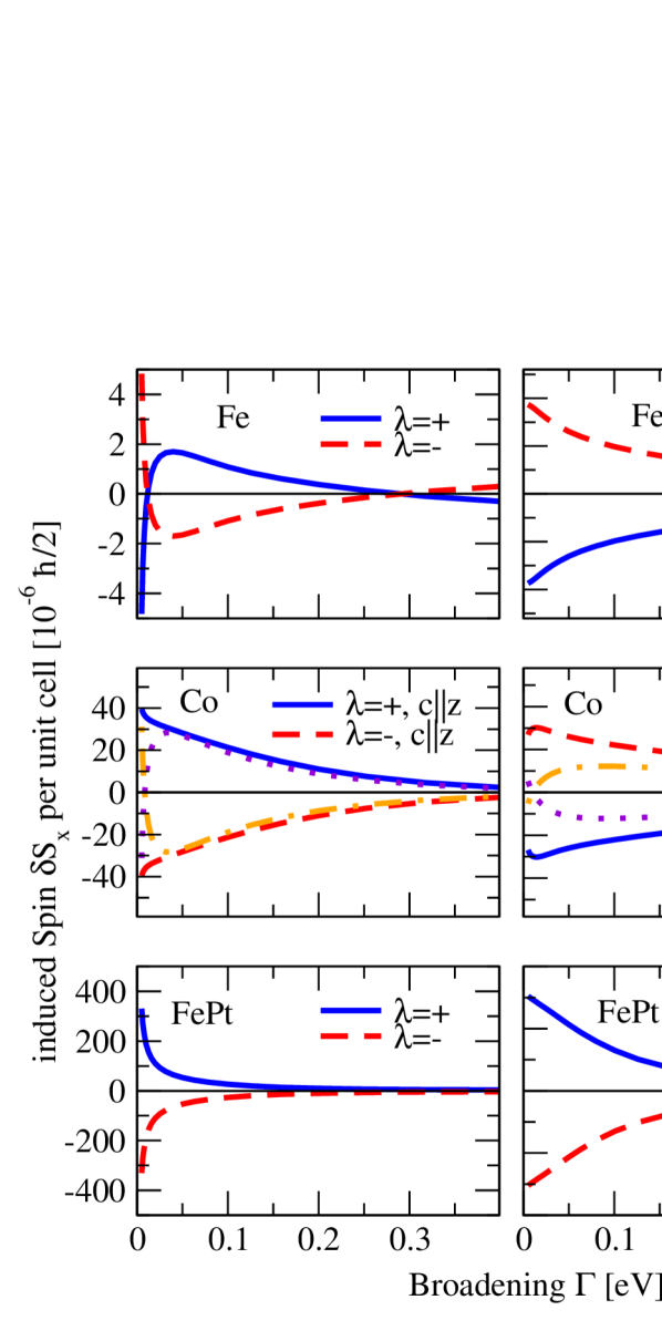
Figure 4: Laser-induced spin polarization $\delta S_{x}$ (left column) and $\delta S_{y}$ (right column) in Fe, Co and FePt as a function of broadening $\Gamma$ at $I=10$ GW/cm². $\hat{{\bm{M}}}$ is in $z$ direction. $\lambda=+$ and $\lambda=-$ denote left and right circularly polarized light, respectively. In the case of Co, results are shown for $c$ axis in $z$ direction ($c\|z$) and $c$ axis in $x$ direction ($c\|x$).

Next, we discuss the laser-induced spin polarization $\delta S_{z}$ along the magnetization direction, which is shown in Figure 5. We find $\delta S_{z}$ to be helicity-independent, in agreement with recent calculations based on the Liouville von-Neumann equation Berritta et al. (2016). Interestingly, $\delta S_{z}$ reaches much larger values than the two perpendicular components $\delta S_{x}$ and $\delta S_{y}$. For example in FePt at $\Gamma$ = 25 meV we find $\delta S_{z}$ = 1.2$\cdot 10^{-2}\hbar/2$ compared to only $\delta S_{x}$ = 9.2$\cdot 10^{-5}\hbar/2$ and $\delta S_{y}$ = 1.3$\cdot 10^{-5}\hbar/2$. In the case of Co $\delta S_{z}$ depends on whether the $c$ axis is in $x$ or $z$ direction, but this anisotropy is less striking than for $\delta S_{x}$ and $\delta S_{y}$ at small $\Gamma$.

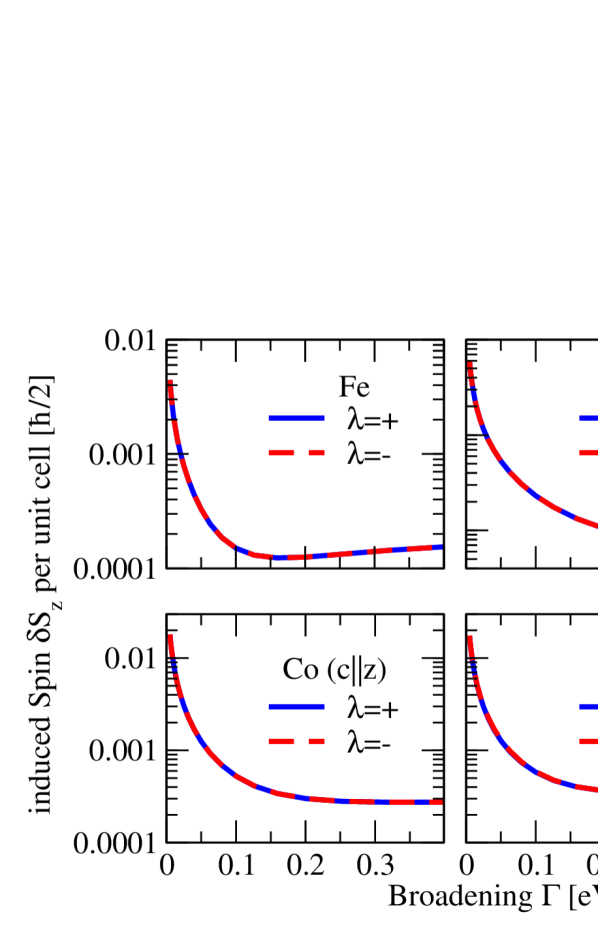
Figure 5: Laser-induced spin polarization $\delta S_{z}$ in Fe, Co and FePt as a function of broadening $\Gamma$ at $I=10$ GW/cm². $\hat{{\bm{M}}}$ is in $z$ direction. $\lambda=+$ and $\lambda=-$ denote left and right circularly polarized light, respectively. In the case of Co, results are shown for $c$ axis in $z$ direction ($c\|z$) and $c$ axis in $x$ direction ($c\|x$).

IV Summary

We combine ab-initio electronic structure calculations with the Keldysh nonequilibrium formalism in order to study laser-induced torques and nonequilibrium spin polarization in bcc Fe, hcp Co and $L1_{0}$ FePt. Our calculations show that both IFE and OSTT are nonzero in these metallic ferromagnets. In the case of Fe the torques due to the OSTT are larger than those due to the IFE, in FePt the IFE dominates over the OSTT and in Co the IFE is dominant only for small and medium quasiparticle broadenings. In view of this strong dependence of the IFE/OSTT ratio on the ferromagnetic material and the quasiparticle broadening (and hence the disorder in the system) it should be possible to design materials such that they display either IFE-torques or OSTT, but not both at the same time. This allows the contactless measurement of various spintronics effect in optical experiments. We find the torques and the perpendicular component of the nonequilibrium spin polarization to be odd in the helicity of the laser light, while the spin polarization that is induced parallel to the magnetization is helicity-independent. This parallel component of the nonequilibrium spin polarization can be orders of magnitude larger than the perpendicular component. The comparison between laser-induced torques and laser-induced nonequilibrium spin density shows the importance of using the torque operator for calculations of laser-induced torques in realistic materials in order to capture the variation of the exchange field on the atomic scale. We find that both the laser-induced torques and the laser-induced nonequilibrium spin polarization are anisotropic in Co. In the case of hcp Co we find good agreement between the calculated laser-induced torque and a recent experiment.

Appendix A Formalism

The Green function $G$ in the presence of the perturbing laser field is obtained from the unperturbed Green function $G_{\rm eq}$ via the Dyson equation on the Keldysh contour Rammer and Smith (1986)

$$G(1,1^{\prime})\!=\!G_{\rm eq}(1,1^{\prime})\!+\!\!\int\!\!{\rm d}\,2\,G_{\rm eq}(1,2)\frac{\delta H(2)}{\hbar}G(2,1^{\prime}),$$ (19)

where $\delta H$ is the perturbation Eq. (2) due to the electric field of the laser. We iterate Eq. (19) to obtain a power series in $\delta H$ and identify the term quadratic in $\delta H$. Applying the Langreth theorem

$$(GGG)^{<}=G^{\rm R}G^{\rm R}G^{<}+G^{\rm R}G^{<}G^{\rm A}+G^{<}G^{\rm A}G^{\rm A}$$ (20)

to the term quadratic in $\delta H$ we obtain:

$$G^{<}_{2}(t,t^{\prime})=$$ (21)

$$\int\!\!{\rm d}t_{1}\!\!\int\!\!{\rm d}t_{2}\,G^{\rm R}_{\rm eq}(t,t_{1})\frac{\delta H(t_{1})}{\hbar}G^{\rm R}_{\rm eq}(t_{1},t_{2})\frac{\delta H(t_{2})}{\hbar}G^{<}_{\rm eq}(t_{2},t^{\prime})+$$

$$\int\!\!{\rm d}t_{1}\!\!\int\!\!{\rm d}t_{2}\,G^{\rm R}_{\rm eq}(t,t_{1})\frac{\delta H(t_{1})}{\hbar}G^{<}_{\rm eq}(t_{1},t_{2})\frac{\delta H(t_{2})}{\hbar}G_{\rm eq}^{\rm A}(t_{2},t^{\prime})+$$

$$\int\!\!{\rm d}t_{1}\!\!\int\!\!{\rm d}t_{2}\,G_{\rm eq}^{<}(t,t_{1})\frac{\delta H(t_{1})}{\hbar}G_{\rm eq}^{\rm A}(t_{1},t_{2})\frac{\delta H(t_{2})}{\hbar}G_{\rm eq}^{\rm A}(t_{2},t^{\prime}).$$

Using

$$G^{\rm R}_{\rm eq}(t,t^{\prime})=\frac{1}{2\pi\hbar}\int_{-\infty}^{\infty}\!\!{\rm d}\mathcal{E}\,{\rm e}^{-i\mathcal{E}(t-t^{\prime})/\hbar}G_{\rm eq}^{\rm R}(\mathcal{E})$$ (22)

and

$$\int_{-\infty}^{\infty}\!\!{\rm d}t_{1}\int_{-\infty}^{\infty}\!\!{\rm d}t_{2}\,{\rm e}^{-\frac{i}{\hbar}\mathcal{E}(t-t_{1})}e^{-i\omega_{1}t_{1}}{\rm e}^{-\frac{i}{\hbar}\mathcal{E}^{\prime}(t_{1}-t_{2})}\times$$ (23)

$$\quad\quad\quad\quad\quad\quad\quad\quad\quad\quad\times e^{-i\omega_{2}t_{2}}{\rm e}^{-\frac{i}{\hbar}\mathcal{E}^{\prime\prime}(t_{2}-t^{\prime})}=$$

$$=h^{2}\delta(\mathcal{E}\!-\!\hbar\omega_{1}\!-\!\mathcal{E}^{\prime})\delta(\mathcal{E}^{\prime}\!-\!\hbar\omega_{2}\!-\!\mathcal{E}^{\prime\prime}){\rm e}^{-\frac{i}{\hbar}\mathcal{E}t}{\rm e}^{\frac{i}{\hbar}\mathcal{E}^{\prime\prime}t^{\prime}}$$

the time-integration of the product of three Green functions can be performed easily:

$$\int\!\!\!{\rm d}t_{1}\!\!\!\int\!\!\!{\rm d}t_{2}G_{\rm eq}^{\alpha}(t,t_{1})e^{-i\omega_{1}t_{1}}G_{\rm eq}^{\alpha^{\prime}}(t_{1},t_{2})e^{-i\omega_{2}t_{2}}G_{\rm eq}^{\alpha^{\prime\prime}}(t_{2},t)=$$ (24)

$$=\frac{{\rm e}^{-i[\omega_{1}+\omega_{2}]t}}{h}\!\int\!\!{\rm d}\mathcal{E}G_{\rm eq}^{\alpha}(\mathcal{E}\!+\!\hbar\omega_{1})G_{\rm eq}^{\alpha^{\prime}}(\mathcal{E})G_{\rm eq}^{\alpha^{\prime\prime}}\!(\mathcal{E}\!-\!\hbar\omega_{2}),$$

where $\alpha,\alpha^{\prime},\alpha^{\prime\prime}={\rm R,A,<}$ and $\omega_{1},\omega_{2}=\pm\omega$. As discussed in section II, we only need the dc component of $G^{<}_{2}$, which arises from all terms with $\omega_{1}=-\omega_{2}=\pm\omega$. It is given by

$$G^{<}_{\rm dc} =\frac{e^{2}E^{2}_{0}}{8\pi\omega^{2}\hbar^{3}}\int{\rm d}\mathcal{E}\Big{\{}$$ (25)

$$G_{\rm eq}^{\rm R}(\mathcal{E}-\hbar\omega){\bm{v}}\cdot\bm{\epsilon}^{*}G_{\rm eq}^{\rm R}(\mathcal{E}){\bm{v}}\cdot\bm{\epsilon}G_{\rm eq}^{<}(\mathcal{E}-\hbar\omega)+$$

$$+ G_{\rm eq}^{\rm R}(\mathcal{E}+\hbar\omega){\bm{v}}\cdot\bm{\epsilon}G_{\rm eq}^{\rm R}(\mathcal{E}){\bm{v}}\cdot\bm{\epsilon}^{*}G_{\rm eq}^{<}(\mathcal{E}+\hbar\omega)+$$

$$+ G_{\rm eq}^{\rm R}(\mathcal{E}-\hbar\omega){\bm{v}}\cdot\bm{\epsilon}^{*}G_{\rm eq}^{<}(\mathcal{E}){\bm{v}}\cdot\bm{\epsilon}G_{\rm eq}^{\rm A}(\mathcal{E}-\hbar\omega)+$$

$$+ G_{\rm eq}^{\rm R}(\mathcal{E}+\hbar\omega){\bm{v}}\cdot\bm{\epsilon}G_{\rm eq}^{<}(\mathcal{E}){\bm{v}}\cdot\bm{\epsilon}^{*}G_{\rm eq}^{\rm A}(\mathcal{E}+\hbar\omega)+$$

$$+ G_{\rm eq}^{<}(\mathcal{E}-\hbar\omega){\bm{v}}\cdot\bm{\epsilon}^{*}G_{\rm eq}^{\rm A}(\mathcal{E}){\bm{v}}\cdot\bm{\epsilon}G_{\rm eq}^{\rm A}(\mathcal{E}-\hbar\omega)+$$

$$+ G_{\rm eq}^{<}(\mathcal{E}+\hbar\omega){\bm{v}}\cdot\bm{\epsilon}G_{\rm eq}^{\rm A}(\mathcal{E}){\bm{v}}\cdot\bm{\epsilon}^{*}G_{\rm eq}^{\rm A}(\mathcal{E}+\hbar\omega)\Big{\}}.$$

Substituting Eq. (25) into Eq. (7) and using

$$G^{<}_{\rm eq}(\mathcal{E})=f(\mathcal{E})\left[G^{\rm A}_{\rm eq}(\mathcal{E})-G^{\rm R}_{\rm eq}(\mathcal{E})\right]$$ (26)

yields

$${\bm{T}}= \frac{ie^{2}E^{2}_{0}}{8\pi\omega^{2}\hbar^{3}}\int{\rm d}\mathcal{E}f(\mathcal{E}){\rm Tr}\Big{\{}$$ (27)

$$\left[{\bm{\mathcal{T}}}R\Lambda^{\dagger}R^{+}\Lambda A\right]-\left[{\bm{\mathcal{T}}}R{\Lambda}^{\dagger}R^{+}{\Lambda}{R}\right]+$$

$$+ \left[{\bm{\mathcal{T}}}{R}{\Lambda}{R}^{-}{\Lambda}^{\dagger}{A}\right]-\left[{\bm{\mathcal{T}}}{R}{\Lambda}{R}^{-}{\Lambda}^{\dagger}{R}\right]+$$

$$+ \left[{\bm{\mathcal{T}}}{R}^{-}{\Lambda}^{\dagger}{A}{\Lambda}{A}^{-}\right]-\left[{\bm{\mathcal{T}}}{R}^{-}{\Lambda}^{\dagger}{R}{\Lambda}{A}^{-}\right]+$$

$$+ \left[{\bm{\mathcal{T}}}{R}^{+}{\Lambda}{A}{\Lambda}^{\dagger}{A}^{+}\right]-\left[{\bm{\mathcal{T}}}{R}^{+}{\Lambda}{R}{\Lambda}^{\dagger}{A}^{+}\right]+$$

$$+ \left[{\bm{\mathcal{T}}}{A}{\Lambda}^{\dagger}{A}^{+}{\Lambda}{A}\right]-\left[{\bm{\mathcal{T}}}{R}{\Lambda}^{\dagger}{A}^{+}{\Lambda}{A}\right]+$$

$$+ \left[{\bm{\mathcal{T}}}{A}{\Lambda}{A}^{-}{\Lambda}^{\dagger}{A}\right]-\left[{\bm{\mathcal{T}}}{R}{\Lambda}{A}^{-}{\Lambda}^{\dagger}{A}\right]\Big{\}},$$

where we introduced the abbreviations $\Lambda={\bm{v}}\cdot\bm{\epsilon}$, $\Lambda^{\dagger}=\left[{\bm{v}}\cdot\bm{\epsilon}\right]^{\dagger}={\bm{v}}\cdot\bm{\epsilon}^{*}$, $R=G^{\rm R}_{\rm eq}(\mathcal{E})$, $A=G^{\rm A}_{\rm eq}(\mathcal{E})$, $R^{+}=G^{\rm R}_{\rm eq}(\mathcal{E}+\hbar\omega)$, $A^{+}=G^{\rm A}_{\rm eq}(\mathcal{E}+\hbar\omega)$, $R^{-}=G^{\rm R}_{\rm eq}(\mathcal{E}-\hbar\omega)$ and $A^{-}=G^{\rm A}_{\rm eq}(\mathcal{E}-\hbar\omega)$. Terms that contain more than one $A$ can be rewritten as complex conjugates of terms with more than one $R$:

$${\bm{T}}=\frac{ie^{2}E^{2}_{0}}{8\pi\omega^{2}\hbar^{3}}\int{\rm d}\mathcal{E}f(\mathcal{E}){\rm Tr}\Big{\{}$$ (28)

$$\left[{\bm{\mathcal{T}}}R\Lambda^{\dagger}R^{+}\Lambda A\right]-\left[{\bm{\mathcal{T}}}R{\Lambda}^{\dagger}R^{+}{\Lambda}{R}\right]+$$

$$+ \left[{\bm{\mathcal{T}}}{R}{\Lambda}{R}^{-}{\Lambda}^{\dagger}{A}\right]-\left[{\bm{\mathcal{T}}}{R}{\Lambda}{R}^{-}{\Lambda}^{\dagger}{R}\right]+$$

$$+ \left[{\bm{\mathcal{T}}}{R}^{-}{\Lambda}^{\dagger}{R}{\Lambda}{A}^{-}\right]^{*}-\left[{\bm{\mathcal{T}}}{R}^{-}{\Lambda}^{\dagger}{R}{\Lambda}{A}^{-}\right]+$$

$$+ \left[{\bm{\mathcal{T}}}{R}^{+}{\Lambda}{R}{\Lambda}^{\dagger}{A}^{+}\right]^{*}-\left[{\bm{\mathcal{T}}}{R}^{+}{\Lambda}{R}{\Lambda}^{\dagger}{A}^{+}\right]+$$

$$+ \left[{\bm{\mathcal{T}}}{R}{\Lambda}^{\dagger}{R}^{+}{\Lambda}{R}\right]^{*}-\left[{\bm{\mathcal{T}}}{R}{\Lambda}^{\dagger}{R}^{+}{\Lambda}{A}\right]^{*}+$$

$$+ \left[{\bm{\mathcal{T}}}{R}{\Lambda}{R}^{-}{\Lambda}^{\dagger}{R}\right]^{*}-\left[{\bm{\mathcal{T}}}{R}{\Lambda}{R}^{-}{\Lambda}^{\dagger}{A}\right]^{*}\Big{\}}.$$

Using the imaginary part to simplify the expression and introducing a Brillouin zone average over $\mathcal{N}$ ${\bm{k}}$ points we finally obtain

$${\bm{T}}= \frac{|e|^{2}E^{2}_{0}}{4\pi\omega^{2}\hbar^{3}\mathcal{N}}\sum_{{\bm{k}}}\int{\rm d}\mathcal{E}{\rm Im}{\rm Tr}\Big{\{}$$ (29)

$$f(\mathcal{E})\left[{\bm{\mathcal{T}}}R_{{\bm{k}}}\Lambda R^{-}_{{\bm{k}}}\Lambda^{\dagger}R_{{\bm{k}}}+{\bm{\mathcal{T}}}R_{{\bm{k}}}\Lambda^{\dagger}R^{+}_{{\bm{k}}}\Lambda R_{{\bm{k}}}\right]$$

$$+ \left[f(\mathcal{E}-\hbar\omega)-f(\mathcal{E})\right]\left[{\bm{\mathcal{T}}}R_{{\bm{k}}}{\Lambda}R^{-}_{{\bm{k}}}{\Lambda}^{\dagger}{A}_{{\bm{k}}}\right]+$$

$$+ \left[f(\mathcal{E}+\hbar\omega)-f(\mathcal{E})\right]\left[{\bm{\mathcal{T}}}{R}_{{\bm{k}}}{\Lambda}^{\dagger}{R}^{+}_{{\bm{k}}}{\Lambda}{A}_{{\bm{k}}}\right]\Big{\}}$$

$$= \frac{a_{0}^{3}I}{c}\left(\frac{\mathcal{E}_{\rm H}}{\hbar\omega}\right)^{2}{\rm Im}\sum_{ijk}\hat{{\bm{e}}}_{i}(\hat{{\bm{e}}}_{j}\cdot\bm{\epsilon})(\hat{{\bm{e}}}_{k}\cdot\bm{\epsilon}^{*})\chi_{ijk},$$

where $\hat{{\bm{e}}}_{1}$, $\hat{{\bm{e}}}_{2}$ and $\hat{{\bm{e}}}_{3}$ are unit vectors along the $x$, $y$ and $z$ axes, respectively. The coefficient $\chi_{ijk}=\chi^{(1)}_{ijk}+\chi^{(2)}_{ijk}$ is given by

$$\chi^{(1)}_{ijk}= \frac{2}{\mathcal{N}\hbar a_{0}^{2}\mathcal{E}_{\rm H}}\sum_{{\bm{k}}}\int{\rm d}\mathcal{E}{\rm Tr}\Big{\{}$$ (30)

$$\left[f(\mathcal{E}-\hbar\omega)-f(\mathcal{E})\right]\left[\mathcal{T}_{i}R_{{\bm{k}}}v_{j}R^{-}_{{\bm{k}}}v_{k}A_{{\bm{k}}}\right]+$$

$$+ \left[f(\mathcal{E}+\hbar\omega)-f(\mathcal{E})\right]\left[\mathcal{T}_{i}{R}_{{\bm{k}}}v_{k}{R}^{+}_{{\bm{k}}}v_{j}{A}_{{\bm{k}}}\right]\Big{\}}$$

and

$$\chi^{(2)}_{ijk}= \frac{2}{\mathcal{N}\hbar a_{0}^{2}\mathcal{E}_{\rm H}}\sum_{{\bm{k}}}\int{\rm d}\mathcal{E}f(\mathcal{E})$$ (31)

$${\rm Tr}\left[\mathcal{T}_{i}R_{{\bm{k}}}v_{j}R^{-}_{{\bm{k}}}v_{k}R_{{\bm{k}}}+\mathcal{T}_{i}R_{{\bm{k}}}v_{k}R^{+}_{{\bm{k}}}v_{j}R_{{\bm{k}}}\right].$$

Appendix B Expressions at $T=0$K

In the present paper we use the constant broadening $\Gamma$ in order to simulate disorder and finite lifetimes of the electronic states. Therefore, the energy dependence of the Green function is known analytically:

$$R_{{\bm{k}}}=G^{\rm R}_{{\bm{k}}}(\mathcal{E})=\hbar\sum_{n}\frac{|{\bm{k}}n\rangle\langle{\bm{k}}n|}{\mathcal{E}-\mathcal{E}_{{\bm{k}}n}+i\Gamma}.$$ (32)

This simple form of $G^{\rm R}_{{\bm{k}}}(\mathcal{E})$ allows us to perform the energy integrations in Eq. (30) and Eq. (31) analytically. We discuss only the zero-temperature limit and therefore replace the Fermi function by the Heaviside step function as $f(\mathcal{E})=\theta(\mathcal{E}_{\rm F}-\mathcal{E})$, where $\mathcal{E}_{\rm F}$ is the Fermi energy. Thus, we need the following two integrals for the evaluation of Eq. (30) and Eq. (31) in the zero-temperature limit:

$$I_{1}(\mathcal{E}_{1},\mathcal{E}_{2},\mathcal{E}_{3},\mathcal{E}_{4})=$$ (33)

$$=\int_{-\infty}^{\mathcal{E}_{4}}\frac{\mathcal{E}^{2}_{\rm H}\quad{\rm d}\mathcal{E}}{(\mathcal{E}-\mathcal{E}_{1}+i\Gamma)(\mathcal{E}-\mathcal{E}_{2}+i\Gamma)(\mathcal{E}-\mathcal{E}_{3}+i\Gamma)}$$

and

$$I_{2}(\mathcal{E}_{1},\mathcal{E}_{2},\mathcal{E}_{3},\mathcal{E}_{4})=$$ (34)

$$=\int_{-\infty}^{\mathcal{E}_{4}}\frac{\mathcal{E}^{2}_{\rm H}\quad{\rm d}\mathcal{E}}{(\mathcal{E}-\mathcal{E}_{1}+i\Gamma)(\mathcal{E}-\mathcal{E}_{2}+i\Gamma)(\mathcal{E}-\mathcal{E}_{3}-i\Gamma)}.$$

In terms of $I_{1}(\mathcal{E}_{1},\mathcal{E}_{2},\mathcal{E}_{3},\mathcal{E}_{4})$ and $I_{2}(\mathcal{E}_{1},\mathcal{E}_{2},\mathcal{E}_{3},\mathcal{E}_{4})$ the coefficients $\chi^{(1)}_{ijk}$ and $\chi^{(2)}_{ijk}$ can be expressed as follows:

$$\chi^{(1)}_{ijk}= \frac{2}{\mathcal{N}}\sum_{{\bm{k}}nmm^{\prime}}{\rm Im}\Bigl{\{}$$ (35)

$$\Bigl{[} I_{2}(\mathcal{E}_{{\bm{k}}m},\mathcal{E}_{{\bm{k}}m^{\prime}}+\hbar\omega,\mathcal{E}_{{\bm{k}}n},\mathcal{E}_{\rm F}+\hbar\omega)-$$

$$I_{2}(\mathcal{E}_{{\bm{k}}m},\mathcal{E}_{{\bm{k}}m^{\prime}}+\hbar\omega,\mathcal{E}_{{\bm{k}}n},\mathcal{E}_{\rm F})\Bigl{]}\mathcal{M}_{ijk}^{nmm^{\prime}}+$$

$$\Bigl{[} I_{2}(\mathcal{E}_{{\bm{k}}m},\mathcal{E}_{{\bm{k}}m^{\prime}}-\hbar\omega,\mathcal{E}_{{\bm{k}}n},\mathcal{E}_{\rm F}-\hbar\omega)-$$

$$I_{2}(\mathcal{E}_{{\bm{k}}m},\mathcal{E}_{{\bm{k}}m^{\prime}}-\hbar\omega,\mathcal{E}_{{\bm{k}}n},\mathcal{E}_{\rm F})\Bigl{]}\mathcal{M}_{ikj}^{nmm^{\prime}}\Bigr{\}}$$

and

$$\chi^{(2)}_{ijk}= \frac{2}{\mathcal{N}}\sum_{{\bm{k}}nmm^{\prime}}{\rm Im}\Bigl{\{}$$ (36)

$$I_{1}(\mathcal{E}_{{\bm{k}}m},\mathcal{E}_{{\bm{k}}m^{\prime}}+\hbar\omega,\mathcal{E}_{{\bm{k}}n},\mathcal{E}_{\rm F})\mathcal{M}_{ijk}^{nmm^{\prime}}+$$

$$I_{1}(\mathcal{E}_{{\bm{k}}m},\mathcal{E}_{{\bm{k}}m^{\prime}}-\hbar\omega,\mathcal{E}_{{\bm{k}}n},\mathcal{E}_{\rm F})\mathcal{M}_{ikj}^{nmm^{\prime}}\Bigr{\}}$$

where

$$\mathcal{M}_{ijk}^{nmm^{\prime}}=\frac{\langle{\bm{k}}n|\mathcal{T}_{i}|{\bm{k}}m\rangle\langle{\bm{k}}m|v_{j}|{\bm{k}}m^{\prime}\rangle\langle{\bm{k}}m^{\prime}|v_{k}|{\bm{k}}n\rangle}{\mathcal{E}_{\rm H}\left[a_{0}\frac{\mathcal{E}_{\rm H}}{\hbar}\right]^{2}}.$$ (37)

The integrations in Eq. (33) and Eq. (34) can be performed analytically. In the general case of $\mathcal{E}_{1}\neq\mathcal{E}_{2}\neq\mathcal{E}_{3}\neq\mathcal{E}_{1}$ we obtain

$$I_{1}(\mathcal{E}_{1},\mathcal{E}_{2},\mathcal{E}_{3},\mathcal{E}_{4})=$$ (38)

$$\frac{\mathcal{E}^{2}_{\rm H}}{2(\mathcal{E}_{1}-\mathcal{E}_{2})(\mathcal{E}_{1}-\mathcal{E}_{3})}\log\left[1+\frac{(\mathcal{E}_{1}-\mathcal{E}_{4})^{2}}{\Gamma^{2}}\right]$$

$$+ \frac{\mathcal{E}^{2}_{\rm H}}{2(\mathcal{E}_{2}-\mathcal{E}_{3})(\mathcal{E}_{2}-\mathcal{E}_{1})}\log\left[1+\frac{(\mathcal{E}_{2}-\mathcal{E}_{4})^{2}}{\Gamma^{2}}\right]$$

$$+ \frac{\mathcal{E}^{2}_{\rm H}}{2(\mathcal{E}_{3}-\mathcal{E}_{1})(\mathcal{E}_{3}-\mathcal{E}_{2})}\log\left[1+\frac{(\mathcal{E}_{3}-\mathcal{E}_{4})^{2}}{\Gamma^{2}}\right]$$

$$+ \frac{\mathcal{E}^{2}_{\rm H}}{i(\mathcal{E}_{1}-\mathcal{E}_{2})(\mathcal{E}_{1}-\mathcal{E}_{3})}\arctan\frac{\mathcal{E}_{4}-\mathcal{E}_{1}}{\Gamma}$$

$$+ \frac{\mathcal{E}^{2}_{\rm H}}{i(\mathcal{E}_{2}-\mathcal{E}_{3})(\mathcal{E}_{2}-\mathcal{E}_{1})}\arctan\frac{\mathcal{E}_{4}-\mathcal{E}_{2}}{\Gamma}$$

$$+ \frac{\mathcal{E}^{2}_{\rm H}}{i(\mathcal{E}_{3}-\mathcal{E}_{1})(\mathcal{E}_{3}-\mathcal{E}_{2})}\arctan\frac{\mathcal{E}_{4}-\mathcal{E}_{3}}{\Gamma}$$

and

$$I_{2}(\mathcal{E}_{1},\mathcal{E}_{2},\mathcal{E}_{3},\mathcal{E}_{4})=$$ (39)

$$\frac{\mathcal{E}^{2}_{\rm H}}{2(\mathcal{E}_{1}-\mathcal{E}_{2})(\mathcal{E}_{1}-\mathcal{E}_{3}-2i\Gamma)}\log\left[1+\frac{(\mathcal{E}_{1}-\mathcal{E}_{4})^{2}}{\Gamma^{2}}\right]$$

$$+ \frac{\mathcal{E}^{2}_{\rm H}}{2(\mathcal{E}_{2}-\mathcal{E}_{3}-2i\Gamma)(\mathcal{E}_{2}-\mathcal{E}_{1})}\log\left[1+\frac{(\mathcal{E}_{2}-\mathcal{E}_{4})^{2}}{\Gamma^{2}}\right]$$

$$+ \frac{\mathcal{E}^{2}_{\rm H}}{2(\mathcal{E}_{3}-\mathcal{E}_{1}+2i\Gamma)(\mathcal{E}_{3}-\mathcal{E}_{2}+2i\Gamma)}\log\left[1+\frac{(\mathcal{E}_{3}-\mathcal{E}_{4})^{2}}{\Gamma^{2}}\right]$$

$$+ \frac{i\mathcal{E}^{2}_{\rm H}}{(\mathcal{E}_{1}-\mathcal{E}_{2})(\mathcal{E}_{3}-\mathcal{E}_{1}+2i\Gamma)}\left[\frac{\pi}{2}+\arctan\frac{\mathcal{E}_{4}-\mathcal{E}_{1}}{\Gamma}\right]$$

$$+ \frac{i\mathcal{E}^{2}_{\rm H}}{(\mathcal{E}_{3}-\mathcal{E}_{2}+2i\Gamma)(\mathcal{E}_{2}-\mathcal{E}_{1})}\left[\frac{\pi}{2}+\arctan\frac{\mathcal{E}_{4}-\mathcal{E}_{2}}{\Gamma}\right]$$

$$+ \frac{i\mathcal{E}^{2}_{\rm H}}{(\mathcal{E}_{3}-\mathcal{E}_{1}+2i\Gamma)(\mathcal{E}_{3}-\mathcal{E}_{2}+2i\Gamma)}\left[\frac{\pi}{2}+\arctan\frac{\mathcal{E}_{4}-\mathcal{E}_{3}}{\Gamma}\right].$$

Due to the energy denominators in Eq. (38), numerical difficulties can arise when $\mathcal{E}_{1}\neq\mathcal{E}_{2}\neq\mathcal{E}_{3}\neq\mathcal{E}_{1}$ is not satisfied. Therefore, when $\mathcal{E}_{1}=\mathcal{E}_{2}\neq\mathcal{E}_{3}$ we use instead of Eq. (38) the expression

$$I_{1}(\mathcal{E}_{1},\mathcal{E}_{1},\mathcal{E}_{3},\mathcal{E}_{4})=$$ (40)

$$\frac{\mathcal{E}^{2}_{\rm H}}{2(\mathcal{E}_{1}-\mathcal{E}_{3})^{2}}\log\left[\frac{\Gamma^{2}+(\mathcal{E}_{3}-\mathcal{E}_{4})^{2}}{\Gamma^{2}+(\mathcal{E}_{1}-\mathcal{E}_{4})^{2}}\right]$$

$$+ \frac{\mathcal{E}^{2}_{\rm H}}{i(\mathcal{E}_{1}-\mathcal{E}_{3})^{2}}\left[\arctan\frac{\mathcal{E}_{4}-\mathcal{E}_{3}}{\Gamma}-\arctan\frac{\mathcal{E}_{4}-\mathcal{E}_{1}}{\Gamma}\right]$$

$$+ \frac{\mathcal{E}^{2}_{\rm H}}{(\mathcal{E}_{3}-\mathcal{E}_{1})(\mathcal{E}_{4}-\mathcal{E}_{1}+i\Gamma)}.$$

Applying $I_{1}(\mathcal{E}_{1},\mathcal{E}_{1},\mathcal{E}_{3},\mathcal{E}_{4})=I_{1}(\mathcal{E}_{1},\mathcal{E}_{3},\mathcal{E}_{1},\mathcal{E}_{4})=I_{1}(\mathcal{E}_{3},\mathcal{E}_{1},\mathcal{E}_{1},\mathcal{E}_{4})$ to Eq. (40) one readily obtains expressions for $I_{1}(\mathcal{E}_{1},\mathcal{E}_{2},\mathcal{E}_{3},\mathcal{E}_{4})$ that can be used in the special cases $\mathcal{E}_{1}\neq\mathcal{E}_{2}=\mathcal{E}_{3}$ or $\mathcal{E}_{1}=\mathcal{E}_{3}\neq\mathcal{E}_{2}$.

Similarly, when $\mathcal{E}_{1}=\mathcal{E}_{2}$, we do not use Eq. (39), but instead

$$I_{2}(\mathcal{E}_{1},\mathcal{E}_{1},\mathcal{E}_{3},\mathcal{E}_{4})=$$ (41)

$$\frac{\mathcal{E}^{2}_{\rm H}}{2(\mathcal{E}_{1}-\mathcal{E}_{3}-2i\Gamma)^{2}}\log\left[\frac{\Gamma^{2}+(\mathcal{E}_{3}-\mathcal{E}_{4})^{2}}{\Gamma^{2}+(\mathcal{E}_{1}-\mathcal{E}_{4})^{2}}\right]$$

$$+ \frac{i\quad\mathcal{E}^{2}_{\rm H}}{(\mathcal{E}_{1}-\mathcal{E}_{3}-2i\Gamma)^{2}}\left[\frac{\pi}{2}+\arctan\frac{\mathcal{E}_{4}-\mathcal{E}_{3}}{\Gamma}\right]$$

$$+ \frac{i\quad\mathcal{E}^{2}_{\rm H}}{(\mathcal{E}_{1}-\mathcal{E}_{3}-2i\Gamma)^{2}}\left[\frac{\pi}{2}+\arctan\frac{\mathcal{E}_{4}-\mathcal{E}_{1}}{\Gamma}\right]$$

$$+ \frac{\mathcal{E}^{2}_{\rm H}}{(\mathcal{E}_{3}-\mathcal{E}_{1}+2i\Gamma)(\mathcal{E}_{4}-\mathcal{E}_{1}+i\Gamma)}.$$

In the special case $\mathcal{E}_{1}=\mathcal{E}_{2}=\mathcal{E}_{3}$ we use

$$I_{1}(\mathcal{E}_{1},\mathcal{E}_{1},\mathcal{E}_{1},\mathcal{E}_{4})=-\frac{\mathcal{E}^{2}_{\rm H}}{2(\mathcal{E}_{4}-\mathcal{E}_{1}+i\Gamma)^{2}}.$$ (42)