Oblique spatial dispersive shock waves in nonlinear Schrödinger flows

Abstract.

In dispersive media, hydrodynamic singularities are resolved by coherent wavetrains known as dispersive shock waves (DSWs). Only dynamically expanding, temporal DSWs are possible in one-dimensional media. The additional degree of freedom inherent in two-dimensional media allows for the generation of time-independent DSWs that exhibit spatial expansion. Spatial oblique DSWs, dispersive analogs of oblique shocks in classical media, are constructed utilizing Whitham modulation theory for a class of nonlinear Schrödinger boundary value problems. Self-similar, simple wave solutions of the modulation equations yield relations between the DSW’s orientation and the upstream/downstream flow fields. Time dependent numerical simulations demonstrate a convective or absolute instability of oblique DSWs in supersonic flow over obstacles. The convective instability results in an effective stabilization of the DSW.

1. Introduction

Breaking of hydrodynamic flows in conservative, weakly dispersive media yields dispersive shock waves (DSWs) characterized by expanding nonlinear wavetrains. Mathematically, a great deal is known about dispersive shock waves in the framework of nonlinear wave modulation theory, also known as Whitham theory [37, 17], and inverse scattering [32, 35, 1] for spatio-temporal (1+1)-dimensional systems (cf. the review [10]). The limited theoretical investigations of DSWs in multiple dimensions [15, 16, 11, 29, 12, 21, 22, 27, 28, 2, 5] and the experimental realization of multi-dimensional DSWs in ultracold atoms as superfluid matter waves [6, 34, 19] and in nonlinear optical diffraction patterns [36, 13] provides motivation for this study of two-dimensional DSWs. Furthermore, with the exception of recent studies on Kadomtsev-Petviashvili and related (2+1)D equations [29, 28, 2, 5], the remaining previous theoretical works invoke asymptotic reductions to the Korteweg-de Vries or (1+1)D nonlinear Schrödinger (NLS) equations. These equations’ complete integrability enables a detailed analytical description via the existence of Riemann invariants for the associated Whitham modulation equations. Whitham theory is applicable to a much wider class of equations and a description of salient DSW features is possible by making a simple wave assumption [7]. In this article, we use simple wave DSW theory (DSW fitting [10]) to construct large amplitude, spatial oblique DSWs for the two-dimensional, time-independent (2+0)D NLS equation. A spatial oblique DSW inhabits a wedge region in the plane filled with stationary, modulated periodic waves. The bounding angles of the oblique DSW are completely determined by the upstream Mach number and the downstream flow angle. Consequently, this asymptotic solution can be applied to the problem of supersonic flow over a corner. We investigate the dynamical stability of an oblique DSW for the corner problem, numerically observing instability. Utilizing the instability theory of oblique dark NLS solitons [26, 22, 25], we classify the convective or absolute nature of the instability. The former provides an effective dynamical stabilization of the oblique DSW near the apex of the corner. Because the 2D NLS equation is an accurate model of nonlinear optical and matter wave dynamics, among other systems, these results exhibit wide application.

1.1. DSW Fitting

Generally, Whitham averaging for an $n^{\textrm{th}}$ order (1+1)D dispersive wave equation proceeds in several steps. The first requirement is an $n$-parameter family of periodic traveling wave solutions. The period and frequency of oscillation determines a length and time scale associated with dispersively initiated dynamic processes. Whitham theory then proceeds by assuming the existence of larger modulation length and time scales on which the traveling wave’s parameters adiabatically vary. The first order, quasi-linear modulation equations for these parameters can be determined by averaging $n-1$ conservation laws associated to the dispersive wave equation. The system is closed by an additional modulation equation, known as the conservation of waves, that results from a consistency condition inherent to the assumption of adiabatic parametric evolution. An important property required for modulational stability of the traveling wave is hyperbolicity of the modulation equations. If the Whitham modulation equations exhibit singularity formation, modulations of quasi-periodic or multiphase solutions may be used, if they exist. In this work, we apply this same procedure to a $5^{\textrm{th}}$ order dispersive (2+0)D spatial system. One of the spatial variables can be viewed as a time-like variable hence, all of the Whitham machinery applies.

Regularization of gradient catastrophe in dispersive hydrodynamics can be asymptotically described utilizing Whitham theory. Away from DSWs, the solution is slowly varying and can be approximately described by the dispersionless equations (dispersionless zone). Shock formation gives rise to the development of oscillations characterized by a modulated traveling wave (oscillation zone). The interfaces between the oscillation and dispersionless zones are unknowns that must be determined along with the solution. Within the oscillation (dispersionless) zone, the Whitham (dispersionless) equations are solved. The two zones are matched at their free boundaries by equating the averaged solution to the dispersionless solution and requiring that either the oscillation amplitude goes to zero (harmonic limit) or the oscillation period goes to infinity (soliton limit). Admissibility criteria analogous to entropy conditions for classical shock waves determine the appropriate limiting behavior. Thus a complete asymptotic description of dispersive hydrodynamics involves the determination of the space-time dynamics of all the modulation parameters and the boundaries between oscillation and dispersionless zones.

This construction may appear to be complex and, perhaps, just as involved as solving the original evolution equation. If one seeks the complete description, this is a challenging problem indeed. However, often one is only interested in the macroscopic physical DSW properties encapsulated by the locations (DSW speeds) and limiting behavior (harmonic or soliton) of the free boundaries. For Riemann step initial data, a DSW fitting method is available under modest assumptions [7, 10]. Remarkably, the DSW speeds and edge properties can be found by integrating two ordinary differential equations (ODEs) that involve only the dispersionless characteristic speeds and the dispersion relation. The integration of the full Whitham equations is not required. In this work, we utilize the DSW fitting method for oblique, spatial NLS DSWs.

We remark that this problem utilizes an unconventional application of Whitham theory. In typical problems, there is either a scalar or system of two governing equations. Here, we have three governing equations, with one of them defining an algebraic relationship in the dispersionless limit.

1.2. Previous Results

One scenario leading to dispersive hydrodynamic singularity formation is a large disturbance, say, in the fluid density. Through a process of self-steepening and dispersive regularization, the disturbance results in unsteady DSWs, which are typically realized along one spatial dimension. The analytical description of DSWs was pioneered by Gurevich and Pitaevskii [17] through the use of Whitham averaging theory [37, 38]. (2+0)D steady oblique DSWs can arise in the long time limit of supersonic flow past a corner. In the weakly nonlinear regime [15, 16, 22], a Korteweg-de Vries (KdV) equation describes the behavior. In the hypersonic [12] regime, hypersonic similitude was used to reduce a (2+0)D steady corner flow problem to a (1+1)D unsteady piston problem [20, 24]. There are also (2+1)D generalizations of (1+1)D DSWs to unsteady oblique DSWs realized by a coordinate rotation [21, 22]. All of these works, except numerical simulations in [27], involved integrable equations (KdV or (1+1)D NLS) enabling a detailed analytical description via the existence of Riemann invariants for the modulation equations. Whitham theory is applicable to a wider class of equations and a description of salient DSW features is possible by making a simple wave assumption [7]. We use this simple wave DSW theory to construct large amplitude oblique DSWs and then investigate their stability in the context of supersonic corner flow.

The layout of the manuscript is as follows. Section 2 provides the formulation of the oblique DSW problem. We develop the necessary tools to apply Whitham theory to the (2+0)D NLS equation in section 3. The asymptotic construction of spatial oblique DSWs is completed in sections 4.1, 4.2 and 4.3 and compared to known small amplitude and hypersonic regimes in sections 4.4 and 4.5. The properties of spatial oblique DSWs are then studied in section 4.6 while their admissibility and instability are studied numerically and analytically in section 4.7. We conclude the manuscript with some discussion in section 5.

2. Problem formulation

We consider the cubic defocusing or repulsive NLS equation in two spatial dimensions

(1) $$i\Psi_{t}=-\frac{1}{2}(\Psi_{xx}+\Psi_{yy})+|\Psi|^{2}\Psi.$$

This equation is a model equation for the order parameter of a Bose-Einstein condensate [33] or the envelope of the optical field propagating through a nonlinear medium [3]. An equivalent representation of the NLS equation can be had through the transformation to dispersive hydrodynamic form ($\Psi=\sqrt{\rho}e^{i\phi}$) so that equation eq. 1 becomes

(2a) $$\rho_{t}+(\rho\phi_{x})_{x}+(\rho\phi_{y})_{y}=0$$

(2b) $$\phi_{t}+\frac{1}{2}|\nabla\phi|^{2}+\rho=D[\rho],$$

(2c) $$D[\rho]=\frac{1}{4}\left(\frac{\rho_{xx}+\rho_{yy}}{\rho}-\frac{\rho_{x}^{2}+\rho_{y}^{2}}{2\rho^{2}}\right).$$

By identifying the phase gradient with a velocity field $\mathbf{u}=(u,v)=\nabla\phi$ and $\rho$ as a density, equation eq. 2a expresses the conservation of mass while equation eq. 2b is an analogue of Bernoulli’s equation. Taking the gradient of equation eq. 2b, we obtain the velocity equations

(3a) $$u_{t}+uu_{x}+vu_{y}+\rho_{x} =D[\rho]_{x}$$

(3b) $$v_{t}+uv_{x}+vv_{y}+\rho_{y} =D[\rho]_{y}.$$

By virtue of potential flow, we also have the irrotationality constraint

(4) $$v_{x}-u_{y}=0.$$

Based on this hydrodynamic representation, it is natural to define the dynamic sound speed $c$ as the speed at which long wavelength, small amplitude density perturbations propagate $c(\rho)=\sqrt{\rho}$. Similarly, we define the Mach number of the flow as

(5) $$M=\frac{|\mathbf{u}|}{\sqrt{\rho}},$$

and the associated Mach angle

(6) $$\mu=\textrm{arcsin}(M^{-1}).$$

We will move freely between the Cartesian velocity components $u$, $v$ and the Mach number $M$ or angle $\mu$ and flow direction

(7) $$\theta=\tan^{-1}(v/u),$$

coordinates.

We are interested in stationary solutions of equation eq. 2 in the form

(8) $$\rho(x,y,t)\to\rho(x,y),\quad\phi(x,y,t)\to-\epsilon t+\phi(x,y),\quad\mathbf{u}(x,y,t)\to\mathbf{u}(x,y),$$

where the constant $\epsilon$ can be interpreted as the superfluid chemical potential [33] or the optical propagation constant [3]. Then equation eq. 2b becomes

(9) $$\frac{1}{2}(u^{2}+v^{2})+\rho-D[\rho] =\epsilon,$$

an analog of Bernoulli’s equation, which implicitly determines $\rho$ in terms of the flow speed $|\mathbf{u}|^{2}$. Equation eq. 9, the steady continuity equation eq. 2a

(10) $$(\rho u)_{x}+(\rho v)_{y}=0,$$

and the irrotationality constraint eq. 4 constitute a closed system for $\rho$, $u$, and $v$. With some algebraic manipulation, this system can be written in the form

(11a) $$\begin{bmatrix}u^{2}-\rho&uv\\ 0&1\end{bmatrix}\begin{bmatrix}u\\ v\end{bmatrix}_{x}+\begin{bmatrix}uv&v^{2}-\rho\\ -1&0\end{bmatrix}\begin{bmatrix}u\\ v\end{bmatrix}_{y} =\begin{bmatrix}\mathbf{u}\cdot\nabla D[\rho]\\ 0\end{bmatrix},$$

(11b) $$\rho =\epsilon-\frac{1}{2}|\mathbf{u}|^{2}+D[\rho].$$

2.1. Corner Boundary Value Problem

The steady equations eq. 11 are supplemented with boundary conditions appropriate for supersonic flow past a corner. Figure 1 provides a schematic for the flow of interest. Without loss of generality, we scale the upstream density to unity and consider an incoming, uniform flow parallel to the $x$ axis with Mach angle $\mu_{1}$. Evaluating equation eq. 11b with these far field conditions as $x\to-\infty$ gives

(12) $$\epsilon=1+\csc^{2}\mu_{1}/2.$$

At all physical boundaries, we apply the condition

(13) $$\mathbf{u}\cdot\mathbf{n}=0,$$

where $\mathbf{n}$ is normal to the boundary. Subsequently, the downstream flow points in the direction of the corner angle $\theta_{2}$ with Mach angle $\mu_{2}$ and density $\rho_{2}$. In the far field downstream flow, we evaluate equation eq. 11b again with eq. 12 to find

(14) $$\rho_{2}=\frac{M_{1}^{2}+2}{M_{2}^{2}+2}=\frac{\sin^{2}\mu_{2}(1+2\sin^{2}\mu_{1})}{\sin^{2}\mu_{1}(1+2\sin^{2}\mu_{2})}.$$

We see that knowledge of the fluid velocity in a steady configuration determines the fluid density via the generalized Bernoulli’s equation eq. 11b as in classical gas dynamics.

Figure 1. Corner boundary value problem for steady, supersonic NLS flow.

Because the upstream and downstream flows exhibit a jump at $x=0$ in the density and velocity field, we can view this steady configuration as a dispersive Riemann problem with “initial” conditions

(15) $$\mu(x,0)=\begin{cases}\mu_{1}&x<0\\ \mu_{2}&x>0\end{cases},\quad\theta(x,0)=\begin{cases}0&x<0\\ \theta_{2}&x>0\end{cases},\quad\rho(x,0)=\begin{cases}1&x<0\\ \rho_{2}&x>0\end{cases},$$

where $\rho_{2}$ is given by eq. 14. We can treat the spatial coordinate $y$ as a time-like variable. As such, we will often use common terminology related to dynamical behavior but the reader is advised to keep in mind that we are considering steady, i.e., time-independent flow configurations. The Riemann problem eq. 15 for equations eq. 11 differs from the classical Riemann problem in that a dispersive regularization is required—i.e., we need to incorporate the dispersive effects encapsulated in the term $D[\rho]$, equation eq. 2c—in contrast to a dissipative regularization. Generically, the Riemann problem for systems is resolved into constant states connected by multiple waves, each of which can be a rarefaction or shock wave [31]. Motivated by the geometry of the problem, it is natural to consider the case where the upstream Mach angle $\mu_{1}$ and deflection angle $\theta_{2}$ are given so that $\mu_{2}$ is to be determined so that the Riemann problem results in a single wave, a simple DSW. This is demonstrated in section 4. Furthermore, we will show in section 3.3 that a necessary condition for the generation of a DSW requires supersonic upstream flow $M_{1}>1$ ($0<\mu_{1}<\pi/2$) and a compressive turn $0<\theta_{2}<\pi/2$. The spatial oblique DSW will be shown to exhibit modulated, periodic waves inside a wedge with bounding angles $\beta_{1}$ and $\beta_{2}$ emanating from the corner (see schematic in fig. 1).

Stated concisely, we seek a large $y$ description of the dispersive Riemann problem eq. 15 for equations eq. 11 that results in a single spatial oblique DSW.

3. Properties of the stationary NLS equation

The application of DSW fitting theory requires knowledge of certain properties of the governing equation [10]. In this section, we present the needed properties.

3.1. Spatially Periodic Solution

Equations eq. 11 admit the periodic wave solution [9]

(16a) $$\rho(x,y) =\rho(\xi)=p_{1}+(p_{2}-p_{1})\,\mathrm{sn}^{2}\left(\sin\varphi\sqrt{p_{3}-p_{1}}\xi;m\right),$$

(16b) $$u(x,y) =d\cos\varphi+\sigma\frac{\sin\varphi\sqrt{p_{1}p_{2}p_{3}}}{\rho(\xi)},$$

(16c) $$v(x,y) =d\sin\varphi-\sigma\frac{\cos\varphi\sqrt{p_{1}p_{2}p_{3}}}{\rho(\xi)},\quad\xi=x-\cot\varphi\,y,\quad m=\frac{p_{2}-p_{1}}{p_{3}-p_{1}},$$

where $\mathrm{sn}$ is the Jacobi elliptic function. This periodic solution has five parameters $0<p_{1}<p_{2}<p_{3}$, $d\in\mathbb{R}$, and $\varphi\in(0,\pi/2)$. Both choices of the sign $\sigma=\pm 1$ give valid solutions corresponding to waves propagating in opposite directions. The angle of constant phase $\xi=\mathrm{const}$ is $\varphi$, measured from the $x$ axis. Recalling that $y$ can be viewed as a time-like variable, $\cot\varphi$ is the “speed” of propagation whereas $\tan\varphi$ is the slope of the wavefronts (lines of constant phase) in the $x$-$y$ plane. Here, $d$ is a free parameter whose physical meaning is the uniform flow velocity along the phase wavefronts; this flow is normal to the direction of wave “propagation” and therefore it does not affect the nonlinear wave profile $\rho(x,y)$. The period of the wave in the $x$ direction is

(17) $$L=\frac{2K(m)}{\sin\varphi\sqrt{p_{3}-p_{1}}},$$

where $K(m)$ is the complete elliptic integral of the first kind. We remark that the oblique periodic wave eq. 16 was generated by simply rotating the zero phase speed, spatially periodic solution of the (1+1)D NLS equation with the addition of an arbitrary flow along the phase wavefronts.

It is convenient to consider a more physically inspired set of parameters that uniquely determine the periodic wave. They are the wavenumber in the $x$ direction $k=2\pi/L$, the density oscillation amplitude $a=p_{2}-p_{1}$, and the mean values $\overline{\rho}$, $\overline{u}$, $\overline{v}$ computed as

(18) $$\overline{f}\equiv\frac{1}{L}\int_{0}^{L}f(\xi)\,\mathrm{d}\xi,$$

leading to

(19) $$\overline{\rho} =p_{3}-(p_{3}-p_{1})\frac{E(m)}{K(m)},$$

(20) $$\overline{u} =d\cos\varphi+\sigma\frac{\sin\varphi\,p_{2}p_{3}}{p_{1}K(m)}\Pi(1-p_{2}/p_{1},m),$$

(21) $$\overline{v} =d\sin\varphi-\sigma\frac{\cos\varphi\,p_{2}p_{3}}{p_{1}K(m)}\Pi(1-p_{2}/p_{1},m),$$

where $E(m)$ and $\Pi(1-p_{2}/p_{1},m)$ are the complete elliptic integrals of the second and third kinds, respectively. An auxiliary variable, the oscillation “frequency”, can be defined as $\omega=k\cot\varphi$.

Dispersive shock waves exhibit two distinct edges: a harmonic wave edge exhibiting small amplitude oscillations and a solitary wave edge. These two features are captured by the solution eq. 16 for appropriate limiting cases [9]. The $k\to 0$ limit yields the stationary oblique soliton solution [8]

(22a) $$\rho(x,y) =\rho(\zeta)=\overline{\rho}-a\,\mathrm{sech}^{2}(\zeta),$$

(22b) $$u(x,y) =\overline{\rho}^{1/2}\overline{M}\left(\cos(\varphi-\overline{\theta})\cos\varphi+\sin(\varphi-\overline{\theta})\sin\varphi\,\frac{\overline{\rho}}{\rho(\zeta)}\right),$$

(22c) $$v(x,y) =\overline{\rho}^{1/2}\overline{M}\left(\cos(\varphi-\overline{\theta})\sin\varphi-\sin(\varphi-\overline{\theta})\cos\varphi\frac{\overline{\rho}}{\rho(\zeta)}\right),$$

(22d) $$\zeta =a^{1/2}\sin\varphi(x-\cot\varphi\,y),$$

where $$\overline{\mathbf{u}}=\overline{\rho}^{1/2}\overline{M}[\cos\overline{\theta},\sin\overline{\theta}]^{T}=[\overline{u},\overline{v}]^{T} \overline{M} \overline{\theta}$$ is the far field flow with , the averaged Mach number eq. 5 and averaged flow angle eq. 7. The amplitude-slope relation

(22e) $$a=\overline{\rho}\left(1-\overline{M}^{2}\sin^{2}(\varphi-\overline{\theta})\right),$$

and the positive density restriction $0<a$ imply

(23) $$|\sin(\varphi-\overline{\theta})|<\sin\overline{\mu},$$

so that the oblique solitary wave is oriented inside the Mach cone defined by the Mach angle $\overline{\mu}$. In contrast, small amplitude dispersive waves exhibit lines of constant phase oriented outside the Mach cone (shown below). The Mach cone is well-known from gas dynamics and represents the spatial region where small amplitude disturbances are confined to propagate in dispersionless, supersonic flow (cf. [4]). This does not contradict the orientation of small amplitude dispersive waves because their propagation direction is orthogonal to the direction of constant phase, hence is outside the Mach cone. These restrictions on wave orientation have been previously described in the context of supersonic NLS flow past a small impurity where oblique solitary waves and dispersive waves are generated [9].

A calculation shows that the $a\to 0$ limit in eq. 16 corresponds to harmonic waves satisfying

(24) $$\rho(x,y) =\overline{\rho}-\frac{a}{2}\cos(kx-\omega y)+\mathcal{O}(a^{2}),$$

(25) $$u(x,y) =\overline{u}+a\frac{\sigma k}{4\overline{\rho}}\left(1+\frac{4\overline{\rho}}{k^{2}+\omega^{2}}\right)^{1/2}\cos(kx-\omega y)+\mathcal{O}(a^{2}),$$

(26) $$v(x,y) =\overline{v}-a\frac{\sigma\omega}{4\overline{\rho}}\left(1+\frac{4\overline{\rho}}{k^{2}+\omega^{2}}\right)^{1/2}\cos(kx-\omega y)+\mathcal{O}(a^{2}),$$

with the dispersion relation

(27) $$\overline{\rho}(k^{2}+\omega^{2})\left(1+\frac{k^{2}+\omega^{2}}{4\overline{\rho}}\right)-(k\overline{u}-\omega\overline{v})^{2}=0.$$

The long wave, stationary sound speed or inverse slope $\lambda=\lim_{k\to 0}\omega/k$ can be found by dividing equation eq. 27 by $k^{2}$ and taking the limit $k\to 0$, leading to the relation

(28) $$\overline{\rho}(1+\lambda^{2})-(\overline{u}-\lambda\overline{v})^{2}=0,$$

whose roots are

(29) $$\begin{split}\lambda_{\pm}&=\frac{\overline{u}\,\overline{v}\mp\sqrt{(\overline{u}^{2}+\overline{v}^{2}-\overline{\rho})\overline{\rho}}}{\overline{v}^{2}-\overline{\rho}}=\cot\left(\overline{\theta}\pm\overline{\mu}\right).\end{split}$$

Thus, as $y$ increases, long stationary waves on the flow $(\overline{\rho},\overline{\mathbf{u}})$ exhibit the “slopes of sound” $1/\lambda_{\pm}$. Real sound slopes coincide with supersonic flow ($\overline{M}>1$) and modulationally stable waves, consistent with hyperbolicity of the dispersionless equations (see section 3.3). Complex sound slopes correspond to subsonic flow and modulational instability, the counterpart of ellipticity for the dispersionless equations.

Figure 2. Admissible vectors $[\omega,k]^{T}=q[\cos\varphi,\sin\varphi]^{T}$ for small amplitude dispersive waves relative to the background flow direction $\overline{\mathbf{u}}$. The shaded region depicts the Mach cone of inadmissible directions defined by the Mach angle $\overline{\mu}=\sin^{-1}(\overline{M}^{-1})$.

It is convenient to consider the dispersion relation eq. 27 in polar coordinates. For this we follow [14] and take

(30) $$k=q\sin\varphi,\quad\omega=q\cos\varphi,\quad\overline{\mathbf{u}}=\overline{\rho}^{1/2}\overline{M}[\cos\overline{\theta},\sin\overline{\theta}].$$

Then equation eq. 27 becomes

(31) $$q=2\overline{\rho}^{1/2}\left(\frac{\sin^{2}(\varphi-\overline{\theta})}{\sin^{2}\overline{\mu}}-1\right)^{1/2}.$$

The dispersion relation eq. 31 is real-valued so long as

(32) $$|\sin(\varphi-\overline{\theta})|\geq\sin\overline{\mu}.$$

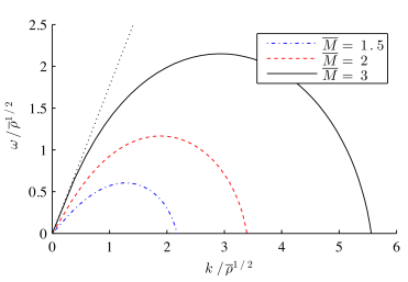
Figure 3. The dispersion relation for several Mach numbers $\overline{M}$ and flow angle $\overline{\theta}=\pi/18$. The dotted line corresponds to the boundary of the Mach cone for $\overline{M}=3$.

This inequality can be interpreted in the following way. The direction of constant phase $[\omega,k]^{T}$, parallel to the dispersive wave troughs and crests, has angle $\varphi$. Inequality eq. 32 is satisfied when $\varphi$ is outside the Mach cone defined by the static sound slope angles $\overline{\theta}\pm\overline{\mu}$ and $\overline{\theta}\pm\overline{\mu}+\pi$ shown in fig. 2. Hence, inequality eq. 32 leads to the admissible angles satisfying

(33) $$\overline{\mu}\leq\left|\varphi-\overline{\theta}\right|\leq\pi-\overline{\mu},$$

in which small amplitude waves satisfying the dispersion relation eq. 27 can propagate. This admissible region is depicted in fig. 2. A branch of the dispersion relation eq. 27 in the $\omega$-$k$ plane for specific choices of $\overline{M}$ is plotted in fig. 3. This primary branch corresponds to $\varphi\in[\overline{\theta}+\overline{\mu},\overline{\theta}+\pi/2]$. The dispersion relation is concave (negative dispersion) across the band $[0,k_{\rm max}]$ of admissible wavenumbers where $k_{\rm max}$ is reached when $\varphi=\pi/2$. The group velocity is

(34) $$\omega_{k}=\frac{\omega_{\varphi}}{k_{\varphi}}=\frac{\sin(2\overline{\theta}-3\varphi)+\cos 2\overline{\mu}\sin\varphi}{\cos(2\overline{\theta}-3\varphi)-\cos 2\mu\cos\varphi},$$

which reaches a zero point for $k_{0}\in(0,k_{\rm max})$.

3.2. Whitham Modulation Equations

Whitham averaging theory describes oscillatory regions by allowing the nonlinear periodic wave solution’s parameters to vary slowly relative to the period of oscillation. The modulation equations can be determined in several, equivalent ways [37, 38]. In DSW theory, it is common to obtain the modulation equations by averaging conservation laws associated to the evolution equation with the periodic wave [10]. For this, we allow the periodic solution’s eq. 16 five parameters to vary according to $(\overline{u},\overline{v},\overline{\rho},a,k)=(\overline{u},\overline{v},\overline{\rho},a,k)(x,y)$. Due to slow variation, any derivatives of the parameters with respect to $x$ or $y$ are considered asymptotically smaller than differentiation of the periodic wave with respect to its phase $\xi$. We begin by averaging equation eq. 9 subject to the periodic wave solution eq. 16

(35) $$\frac{1}{2}(\overline{u^{2}}+\overline{v^{2}})+\overline{\rho}-\overline{D[\rho]}=\epsilon,$$

recalling the definition of nonlinear wave averaging eq. 18. This provides a global relation for the modulation parameters, thus reducing the number of required conservation laws by one. Because of this, we can view the mean density $\overline{\rho}$ as an auxiliary variable, determined from eq. 35 by the variations of the other parameters. Three more equations are found by averaging the continuity equation eq. 10, the irrotationality constraint eq. 4, and the stationary energy equation [23]

(36a) $$\nabla\cdot(\overline{\rho\mathbf{u}}) =0,$$

(36b) $$(\overline{v})_{x}+(\overline{u})_{y} =0,$$

(36c) $$\nabla\cdot\left(\overline{\mathbf{u}\left(\mathcal{E}+\rho^{2}/2\right)}-\overline{\mathbf{u}\Delta\rho/4}+\overline{(\nabla\rho)(\nabla\cdot(\rho\mathbf{u}))/(4\rho)}\right) =0.$$

where the energy $\mathcal{E}$ is

(37) $$\mathcal{E}=\frac{1}{2}\rho(u^{2}+v^{2})+\frac{|\nabla\rho|^{2}}{8\rho}+\frac{1}{2}\rho^{2}.$$

The final modulation equation is the conservation of waves,

(38) $$k_{y}+\omega_{x}=0,$$

a consistency condition for the assumption of slow modulations [38].

The modulation equations eq. 35, eq. 36, and eq. 38 provide a closed system for the spatial evolution of the periodic wave’s five parameters. In order to construct the DSW, we need to assign appropriate initial/boundary data to the modulation equations compatible with the Riemann data eq. 15. This will be achieved in section 4.

3.3. Dispersionless Regime

The application of DSW theory requires knowledge of the dispersionless limiting equations ($D\to 0$ in equations eq. 11), which we can write as

(39a) $$\begin{bmatrix}u\\[8.53581pt] v\end{bmatrix}_{y}+\begin{bmatrix}0&-1\\ \frac{u^{2}-\rho}{v^{2}-\rho}&\frac{2uv}{v^{2}-\rho}\end{bmatrix}\begin{bmatrix}u\\[8.53581pt] v\end{bmatrix}_{x} =0,$$

(39b) $$\rho+\frac{1}{2}|\mathbf{u}|^{2} =\epsilon.$$

This quasi-linear system has been well-studied in the context of gas dynamics (cf. [4]). It exhibits the same characteristic speeds $\lambda_{\pm}=\cot(\theta\pm\mu)$ as resulted from the long wavelength limit eq. 29. The system eq. 39a is strictly hyperbolic and genuinely nonlinear when the characteristic speeds are real, i.e., when the flow is supersonic. Equations eq. 39a are diagonalized by the Riemann invariants

(40) $$s_{\pm}(\theta,\mu)=\theta\pm\left(-\mu+\sqrt{3}\tan^{-1}(\sqrt{3}\tan\mu)\right).$$

Simple wave solutions correspond to changes in only one Riemann invariant

(41) $$s_{\pm}=\mathrm{const}\quad\mathrm{and}\quad\lambda_{\mp}=x/y.$$

These solutions exhibit flows with an expansion turn forming a rarefaction wave. The Riemann initial data eq. 15 for the dispersionless equations eq. 39a exhibits a single rarefaction wave when

(42) $$s_{-}(0,\mu_{1})<\theta_{2}<0.$$

This is the Prandtl-Meyer expansion fan [4]. When the flow turns too much, $\theta_{2}<s_{-}(0,\mu_{1})$, it exhibits cavitation ($\rho\to 0$).

The dispersionless equations eq. 39 exhibit gradient catastrophe when the flow experiences a compressive turn. For the Riemann data eq. 15, this corresponds to $\theta_{2}>0$. In gas dynamics, the singularity is resolved by appealing to small scale physical processes coinciding with dissipation. In the next section, we resolve singularity formation utilizing a dispersive regularization due to nonzero $D[\rho]$ in equations eq. 11.

4. Oblique DSWs

As described in section 1.1, a complete description of spatial DSWs requires integration of the Whitham equations eq. 35, eq. 36, and eq. 38 matched to the dispersionless flow satisfying eq. 39. As originally formulated by Gurevich and Pitaevskii in the KdV DSW problem [17], matching corresponds to equality of the dispersionless $(u,v,\rho)$ and averaged $(\overline{u},\overline{v},\overline{\rho})$ flow variables at the edges of the DSW. Embedded within this matching procedure is the requirement that two characteristics of the Whitham equations coalesce, which occurs when either $a\to 0$ (harmonic wave edge) or $k\to 0$ (solitary wave edge). The remaining modulation parameter determines the location of the interface. At the harmonic wave edge, the nonzero wavenumber corresponds to a wave packet moving with the group velocity. The solitary wave edge moves according to the phase speed of a solitary wave with amplitude $a$. The specific choice of Riemann data eq. 15 implies self-similar behavior for the modulations so it is natural to seek a simple wave solution of the modulation equations. The innovation in [7] was the determination of the DSW edge locations while bypassing full integration of the modulation equations. This was achieved by a priori assuming the existence of a simple wave and analyzing the modulation equations in the $a\to 0$ and $k\to 0$ limits. This analysis results in a universal description of simple DSW edge speeds.

In section 3 we provided all the necessary pieces in order to implement Whitham averaging. However, it is important to note that the simple DSW construction presented in [7] can be implemented with knowledge of only the linear dispersion relation eq. 27, the dispersionless characteristic speeds eq. 29, and the solitary wave amplitude/speed relation eq. 22e. This reflects the fact that a DSW incorporates a range of nonlinear wave phenomena, from large amplitude solitary waves to vanishingly small amplitude waves, into a single coherent structure. The integration of the universal, simple DSW ODEs show how the harmonic and solitary wave edges are nonlocally connected.

4.1. DSW Locus

The assumption of a simple wave solution to the full modulation system yields several important results. Utilizing a backward characteristic argument, it was shown that the Riemann data eq. 15 coincides with a single DSW opening to the right when [7]

(43) $$s_{-}(0,\mu_{1})=s_{-}(\theta_{2},\mu_{2}).$$

This is a 2-DSW, named thus because it degenerates to the faster characteristic speed $\lambda_{+}$ in the small amplitude regime [10]. This provides an explicit relationship between the upstream and downstream flow variables that must hold for a 2-DSW. In combination with two expansion fan solutions and 1-DSWs, these four wave types form the generic building blocks for the general solution to the Riemann problem. See [10] for additional details. The locus eq. 43 enables the determination of the sonic curve, i.e., the relationship between $\mu_{1}$ and $\theta_{2}$ such that $M_{2}=1$ or, equivalently, $\mu_{2}=\pi/2$. We define the sonic angle $\theta_{\rm s}$ according to $s_{-}(0,\mu_{1})=\lim_{\mu_{2}\to\pi/2^{-}}s_{-}(\theta_{\rm s},\mu_{2})$, obtaining

(44) $$\theta_{\rm s}(\mu_{1})=\left(\sqrt{3}-1\right)\frac{\pi}{2}+\mu_{1}-\sqrt{3}\tan^{-1}\left(\sqrt{3}\tan\mu_{1}\right).$$

For an oblique DSW with $0<\mu_{1}<\pi/2$, the dispersionless quasi-linear system eq. 39a is hyperbolic if and only if $0\leq\theta_{2}<\theta_{\rm s}$.

In addition to the DSW locus eq. 43, a local, simple wave relation holds when either $a=0$ or $k=0$ [7, 10]

(45) $$s_{-}(0,\mu_{1})=s_{-}(\overline{\theta},\overline{\mu}),\quad 0<\overline{\theta}(\overline{\mu})<\theta_{2},$$

leading to

(46) $$\overline{\theta}=\overline{\theta}(\overline{\mu})=\mu_{1}-\overline{\mu}-\sqrt{3}\left[\tan^{-1}(\sqrt{3}\tan\mu_{1})-\tan^{-1}(\sqrt{3}\tan\overline{\mu})\right].$$

Similarly, when $a=0$ or $k=0$ equation eq. 35 implies the local relation

(47) $$\overline{\rho}=\overline{\rho}(\overline{\mu})=\frac{\sin^{2}\overline{\mu}\,(1+2\sin^{2}\mu_{1})}{\sin^{2}\mu_{1}\,(1+2\sin^{2}\overline{\mu})}.$$

We can evaluate the density between the oblique DSW and the wedge as

(48) $$\rho_{2}=\overline{\rho}(\mu_{2})=\frac{\sin^{2}\mu_{2}(1+2\sin^{2}\mu_{1})}{\sin^{2}\mu_{1}(1+2\sin^{2}\mu_{2})}.$$

4.2. Harmonic Wave Edge Angle

The angle $\beta_{1}$ (recall fig. 1) of the harmonic wave edge ($a=0$) is determined by integrating the simple wave ordinary differential equation [7]

(49) $$\frac{\mathrm{d}k}{\mathrm{d}\overline{\mu}}=\frac{\omega_{\overline{\mu}}(k,\overline{\mu})}{\lambda_{+}(\overline{\mu})-\omega_{k}(k,\overline{\mu})},\quad k(\mu_{2})=0,$$

to $k_{1}=k(\mu_{1})$ and then evaluating the group velocity

(50) $$\beta_{1}=\cot^{-1}\omega_{k}(k_{1},\mu_{1}).$$

This represents an integration from the solitary wave edge $(\overline{\mu},\overline{\theta},\overline{\rho},k,a)=$ $(\mu_{2},\theta_{2},\rho_{2},0,a_{2})$ to the harmonic wave edge $(\overline{\mu},\overline{\theta},\overline{\rho},k,a)=(\mu_{1},0,1,k_{1},0)$. The integration is accomplished while remaining in the $a=0$ plane. Let us see why this is so. The assumed existence of a simple wave necessitates a functional relationship between the modulation variables $F(\overline{\mu},\overline{\theta},\overline{\rho},k,a)=C$ where $C\in\mathbb{R}$ is a constant. Then, $C$ is implicitly determined by $F(\mu_{2},\theta_{2},\rho_{2},0,a_{2})=C$ from the soliton edge initial condition $k(\mu_{2})=0$ when $\overline{\mu}=\mu_{2}$, $\overline{\theta}=\theta_{2}$, and $\overline{\rho}=\rho_{2}$. But the initial condition is independent of $a$ so the functional relationship $F(\mu_{2},\theta_{2},\rho_{2},0,0)=C$ must also hold and determines $C$. Then $k_{1}$ is found by evaluating $F(\mu_{1},0,1,k_{1},0)=C$ via integration of eq. 49 in the $a=0$ plane, thus bypassing the integration of the full Whitham system.

Due to the implicit nature of the dispersion relation eq. 27, we undertake the solution of eq. 49 utilizing the polar form eq. 30, eq. 31. The transformation of eq. 49 into polar form is somewhat involved. We relegate the details to section A.1. The harmonic edge initial value problem then becomes

(51) $$\frac{\mathrm{d}\varphi}{\mathrm{d}\overline{\mu}}=\frac{2\cos\overline{\mu}\left[2\sin\overline{\mu}-\sin(2\overline{\theta}+\overline{\mu}-2\varphi)\right]}{(2-\cos 2\overline{\mu})\left[\sin(2\overline{\mu})-2\sin(2\overline{\theta}-2\varphi)\right]},\quad\varphi(\mu_{2})=\overline{\theta}(\mu_{2})+\mu_{2},$$

where $\overline{\theta}(\overline{\mu})$ satisfies the local relation eq. 45. Integrating this to $\overline{\mu}=\mu_{1}$ and evaluating eq. 50 provides the harmonic edge angle.

4.3. Solitary Wave Edge Angle

The angle $\beta_{2}$ (recall fig. 1) of the solitary wave edge ($k=0$) can be formulated in an analogous way to the harmonic edge by the introduction of new modulation variables $(k,\omega)\to(\tilde{k},\tilde{\omega})$ via

(52) $$\tilde{\omega}(\tilde{k},\overline{\mu})=-i\omega(i\tilde{k},\overline{\mu}).$$

The conjugate wavenumber $\tilde{k}$ plays the role of an amplitude and is a convenient parameterization of the periodic traveling wave, which leads to the simple wave initial value problem [7]

(53) $$\frac{\mathrm{d}\tilde{k}}{\mathrm{d}\overline{\mu}}=\frac{\tilde{\omega}_{\overline{\mu}}(\tilde{k},\overline{\mu})}{\lambda_{+}(\overline{\mu})-\tilde{\omega}_{\tilde{k}}(\tilde{k},\overline{\mu})},\quad\tilde{k}(\mu_{1})=0.$$

Note the symmetry of equations eq. 49 and eq. 53. Upon integration of eq. 53 to $\tilde{k}_{2}=\tilde{k}(\mu_{2})$, the solitary wave edge angle is determined from the solitary wave phase speed $\tilde{\omega}/\tilde{k}$ according to

(54) $$\beta_{2}=\cot^{-1}\frac{\tilde{\omega}(\tilde{k}_{2},\mu_{2})}{\tilde{k}_{2}}.$$

The solution of equation eq. 53 represents the integration from the harmonic wave edge to the solitary wave edge in the $k=0$ plane in an analogous manner to the harmonic edge case. As shown in section A.2, this problem can be cast in the form

(55) $$\frac{\mathrm{d}\tilde{\varphi}}{\mathrm{d}\overline{\mu}} =\frac{2\cos\overline{\mu}\left[2\sin\overline{\mu}-\sin(2\overline{\theta}+\overline{\mu}-2\tilde{\varphi})\right]}{(2-\cos 2\overline{\mu})\left[\sin(2\overline{\mu})-2\sin(2\overline{\theta}-2\tilde{\varphi})\right]},\quad\tilde{\varphi}(\mu_{1})=\overline{\theta}(\mu_{1})+\mu_{1}=\mu_{1},$$

where $\overline{\theta}(\overline{\mu})$ satisfies eq. 45. Integrating to $\overline{\mu}=\mu_{2}$ and evaluating eq. 54 provides the soliton edge angle.

4.4. Small Amplitude Regime

The small amplitude regime was studied in [22] by an asymptotic reduction of the (2+0)D NLS equation eq. 11 to the KdV equation. This regime corresponds to small deflection angles $0<\theta_{2}\ll 1$ with $M_{1}=\mathcal{O}(1)$, to distinguish it from the hypersonic regime studied in the next section. Here, we perform an asymptotic analysis of the Whitham modulation equations for the full (2+0)D equations to verify the validity of our results and to provide an alternative derivation. Evaluating the DSW locus eq. 45 in this regime implies

(56) $$\overline{\theta}(\overline{\mu})=\frac{2(\overline{\mu}-\mu_{1})}{1+3\tan^{2}\mu_{1}}+\mathcal{O}((\overline{\mu}-\mu_{1})^{2}),$$

which gives $\theta_{2}=\overline{\theta}(\mu_{2})$. This relation can be inverted to give

(57) $$\overline{\mu}(\overline{\theta})=\mu_{1}+\frac{1}{2}(1+3\tan^{2}\mu_{1})\overline{\theta}+\mathcal{O}(\overline{\theta}^{2}).$$

We also recover the asymptotic density variation

(58) $$\overline{\rho}(\overline{\theta})=1+2\csc(2\mu_{1})\overline{\theta}+\mathcal{O}(\overline{\theta}^{2}).$$

Both eq. 57 and eq. 58 agree with the results in [22] when $\overline{\theta}=\theta_{2}$.

Since $0<\overline{\theta}\ll 1$, the restriction eq. 33 implies $\varphi-\mu_{1}=\mathcal{O}(\overline{\theta})$ in the parametric representation of the dispersion relation. It is convenient to utilize the independent variable $\overline{\theta}$ in the simple wave initial value problem eq. 51 rather than $\overline{\mu}$, achieved through the relation eq. 56. Then, for $0<\overline{\theta}\ll 1$, eq. 51 becomes

(59) $$\frac{\mathrm{d}\varphi}{\mathrm{d}\overline{\theta}}=\frac{1}{2}\sec^{2}\mu_{1},\quad\varphi(\theta_{2})=\theta_{2}+\mu_{2}.$$

The solution evaluated at the harmonic edge, $\overline{\theta}=0$, yields $\varphi_{1}\equiv\varphi(0)=\mu_{2}+(1-\frac{1}{2}\sec^{2}\mu_{1})\theta_{2}$. Now we recover the harmonic edge angle from equation eq. 50

(60) $$\beta_{1}=\cot^{-1}\omega_{k}(k_{1},\mu_{1})=\cot^{-1}\frac{\omega_{\varphi}(\varphi_{1},\mu_{1})}{k_{\varphi}(\varphi_{1},\mu_{1})}=\mu_{1}+3\sec^{2}\mu_{1}\theta_{2}.$$

The soliton edge simple wave problem reduces similarly to

(61) $$\frac{\mathrm{d}\tilde{\varphi}}{\mathrm{d}\overline{\theta}}=\frac{1}{2}\sec^{2}\mu_{1},\quad\tilde{\varphi}(0)=\mu_{1}.$$

Evaluating at $\overline{\theta}=\theta_{2}$ and inserting into eq. 54 gives

(62) $$\beta_{2}\sim\mu_{1}+\frac{1}{2}\sec^{2}\mu_{1}\theta_{2}.$$

Both eq. 60 and eq. 62 agree with the alternative approach in [22].

4.5. Hypersonic Regime

The hypersonic regime $M_{1}\gg 1$, $\theta_{2}\ll 1$ such that $M_{1}\theta_{2}=\mathcal{O}(1)$, or, equivalently $0<\mu_{1}\sim\theta_{2}\ll 1$, was studied in [12] by an asymptotic reduction of the (2+0)D NLS equation to a (1+1)D NLS equation. One might naively try to utilize the small amplitude results from the prior section with $\mu_{1}$ small. However, this does not provide the correct results. We now recover the hypersonic results through asymptotics of the Whitham modulation equations. When $0<\overline{\mu}\ll 1$, the DSW locus eq. 43 yields the simple wave relation

(63) $$\theta_{2}\sim 2(\mu_{2}-\mu_{1}),\quad 0<\mu_{i}\ll 1.$$

Since $\overline{\theta}$ and $\overline{\mu}$ are small, we observe from eq. 33 that $\varphi=\mathcal{O}(\overline{\mu})$. The simple wave initial value problem for the harmonic edge eq. 51 asymptotically simplifies tremendously to

(64) $$\frac{\mathrm{d}\varphi}{\mathrm{d}\overline{\mu}}=1,\quad\varphi(\mu_{2})=3\mu_{2}-2\mu_{1}.$$

Solving equation eq. 64 and evaluating at the harmonic wave edge we obtain $\varphi_{1}\equiv\varphi(\mu_{1})=2\mu_{2}-\mu_{1}$. Inserting this result into equation eq. 50 yields the harmonic edge angle

(65) $$\beta_{1}=\cot^{-1}\omega_{k}(k_{1},\mu_{1})=\cot^{-1}\frac{\omega_{\varphi}(\varphi_{1},\mu_{1})}{k_{\varphi}(\varphi_{1},\mu_{1})}\sim\frac{\mu_{1}^{2}+4\mu_{1}\theta_{2}+2\theta_{2}^{2}}{\theta_{2}+\mu_{1}}.$$

Utilizing the asymptotic substitution $\mu_{1}\sim 1/M_{1}$, the result eq. 65 was also found in [12].

The soliton edge is analyzed in a similar way for $0<\overline{\mu}\ll 1$, resulting in the simple wave ODE

(66) $$\frac{\mathrm{d}\tilde{\varphi}}{\mathrm{d}\overline{\mu}}=1,\quad\tilde{\varphi}(\mu_{1})=\mu_{1},$$

with solution $\tilde{\varphi}(\overline{\mu})=\overline{\mu}$. Then $\tilde{\varphi}_{2}\equiv\tilde{\varphi}(\mu_{2})=\mu_{2}$ and equation eq. 54 yield the soliton edge angle

(67) $$\beta_{2}=\cot^{-1}\frac{\tilde{\omega}(\tilde{k}_{2},\mu_{2})}{\tilde{k}_{2}}=\cot^{-1}\frac{\tilde{q}(\tilde{\varphi}_{2},\mu_{2})\cos\tilde{\varphi}_{2}}{\tilde{q}(\tilde{\varphi}_{2},\mu_{2})\sin\tilde{\varphi}_{2}}\sim\mu_{2}\sim\mu_{1}+\frac{1}{2}\theta_{2},$$

which agrees with [12].

4.6. Simple Oblique DSW

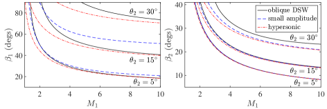
Figure 4. Oblique DSW angles versus upstream Mach number for three values of the flow angle $\theta_{2}$. These plots highlight the limitations of the small amplitude (dashed) and hypersonic (dash-dotted) asymptotic regimes when compared with the full construction (solid).

In order to investigate oblique DSWs across a wide parameter regime, we numerically solve the ODEs eq. 51 and eq. 53, utilizing the DSW locus eq. 43, for the oblique DSW angles $\beta_{1}$ and $\beta_{2}$, respectively as well as for the downstream flow properties. The problem as formulated (cf. fig. 1) involves two free parameters, which we choose to be the upstream Mach number $M_{1}$ and the downstream flow angle $\theta_{2}$. These are the two natural input parameters for supersonic flow past a corner.

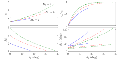
Figure 5. Oblique DSW parameters for fixed upstream Mach number $M_{1}=2$ (solid), $M_{1}=3$ (dashed), $M_{1}=4$ (dash-dotted). Both $\beta_{1}$ and $\beta_{2}$ are plotted in the lower-right panel ($\beta_{1}>\beta_{2}$). Numerically extracted quantities from supersonic flow over a corner are filled circles.

First we compare predictions for the oblique DSW angles $\beta_{1,2}$ with the small amplitude and hypersonic predictions from section 4.4 and section 4.5, respectively in fig. 4. Recall that both asymptotic regimes require $0<\theta_{2}\ll 1$ and either $M_{1}=\mathcal{O}(1)$ or $M_{1}\theta_{2}=\mathcal{O}(1)$ in the small amplitude or hypersonic regime, respectively. The regimes of validity are borne out by our computations although the soliton edge angle $\beta_{2}$ exhibits better than expected agreement with the asymptotics.

Representative results for the full oblique DSW construction are shown in fig. 5 and fig. 6. Several features are noticeable. In both figures, the oblique DSW ceases to exist when the downstream flow is subsonic, $M_{2}<1$. The dispersionless equations eq. 39 are elliptic in the subsonic regime so our construction is no longer valid. In fig. 6, we observe that the DSW soliton edge amplitude saturates ($a_{\rm s}=\rho_{2}$) for both $\theta_{2}=20^{\circ}$ and $\theta_{2}=25^{\circ}$. This soliton amplitude saturation corresponds to cavitation or the development of a region of zero density. A more careful examination shows that saturation occurs when the downstream flow angle and DSW soliton edge angle coincide $\theta_{2}=\beta_{2}$. Further increase of the flow angle $\theta_{2}$ requires a modification of the DSW fitting procedure. This modification was carried out in the hypersonic regime [12] but we do not do so here.

We further explore parameter space with time-dependent numerical simulations of supersonic flow past a corner. We incorporate a time-dependent linear potential in the NLS equation eq. 1 that models the effect of a corner with angle $\theta_{2}$ moving through a confined fluid. Initial data corresponds to the steady state within a static confining potential. For $t>0$, the corner moves at a constant speed determined by $M_{1}$. A sufficiently large domain was used to resolve the development of oblique DSWs with a grid spacing of $0.25$ for a pseudospectral-Fourier spatial discretization and fourth order Runge-Kutta time-stepping. The numerical method is described in detail in [22].

Figure 5 and fig. 6 include a comparison of direct numerical simulations applied to the asymptotic theory, yielding excellent agreement. There are restrictions on the validity of the asymptotic theory, which we now discuss in the next subsection.

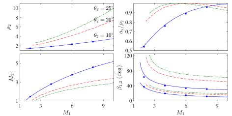
Figure 6. Oblique DSW parameters for fixed corner angle $\theta_{2}=10^{\circ}$ (solid), $\theta_{2}=20^{\circ}$ (dashed), $\theta_{2}=25^{\circ}$ (dash-dotted). Numerically extracted quantities from supersonic flow over a corner are filled circles.

4.7. Admissibility

For a DSW approximated by the DSW fitting method, as herein, it must satisfy certain causality conditions and admissibility criteria [10]. The causality conditions for an oblique DSW ensure that the second, dispersionless characteristic family associated with $\lambda_{+}$ carries data into the DSW region. They are

(68) $$\lambda_{-}(0,\mu_{1})<\cot\beta_{1}<\lambda_{+}(0,\mu_{1}),\quad\lambda_{+}(\theta_{2},\mu_{2})<\cot\beta_{2},\quad\beta_{1}>\beta_{2}.$$

These conditions have been verified in the small amplitude [22] and hypersonic [12] regimes. We have numerically verified these relations to hold for $0<\theta_{2}<\pi/2$ and $1<M_{1}<20$ when $1<M_{2}$, i.e., for supersonic downstream flow.

The DSW fitting method breaks down when the underlying assumption of the existence of a simple wave solution to the Whitham equations no longer holds [18]. Two possible mechanisms for such a breakdown are a loss of genuine nonlinearity in the Whitham equations or zero dispersion, which ultimately result from a loss of monotonicity. Because it incorporates exact reductions of the Whitham equations at the harmonic and soliton edges, the DSW fitting method provides a means to test for simple wave breakdown at the DSW edges. Breakdown manifests at a DSW edge when its speed, or angle in our case, experiences an extremum as one of the edge parameters is varied [18, 10]. We find that $\beta_{2}(M_{1},M_{2})$, with $M_{2}$ fixed, exhibits a minimum when $M_{1}=M_{\rm gnl}(M_{2})$. This minimum corresponds to the occurrence of a linearly degenerate point or the loss of genuine nonlinearity at the oblique DSW soliton edge. For $M_{1}>M_{\rm gnl}(M_{2})$, the simple wave assumption no longer holds, placing a restriction on the validity of the DSW fitting method. We have also computed $\beta_{1}$ with fixed $M_{2}$ and $\beta_{1,2}$ with fixed $M_{1}$ and find no extremum.

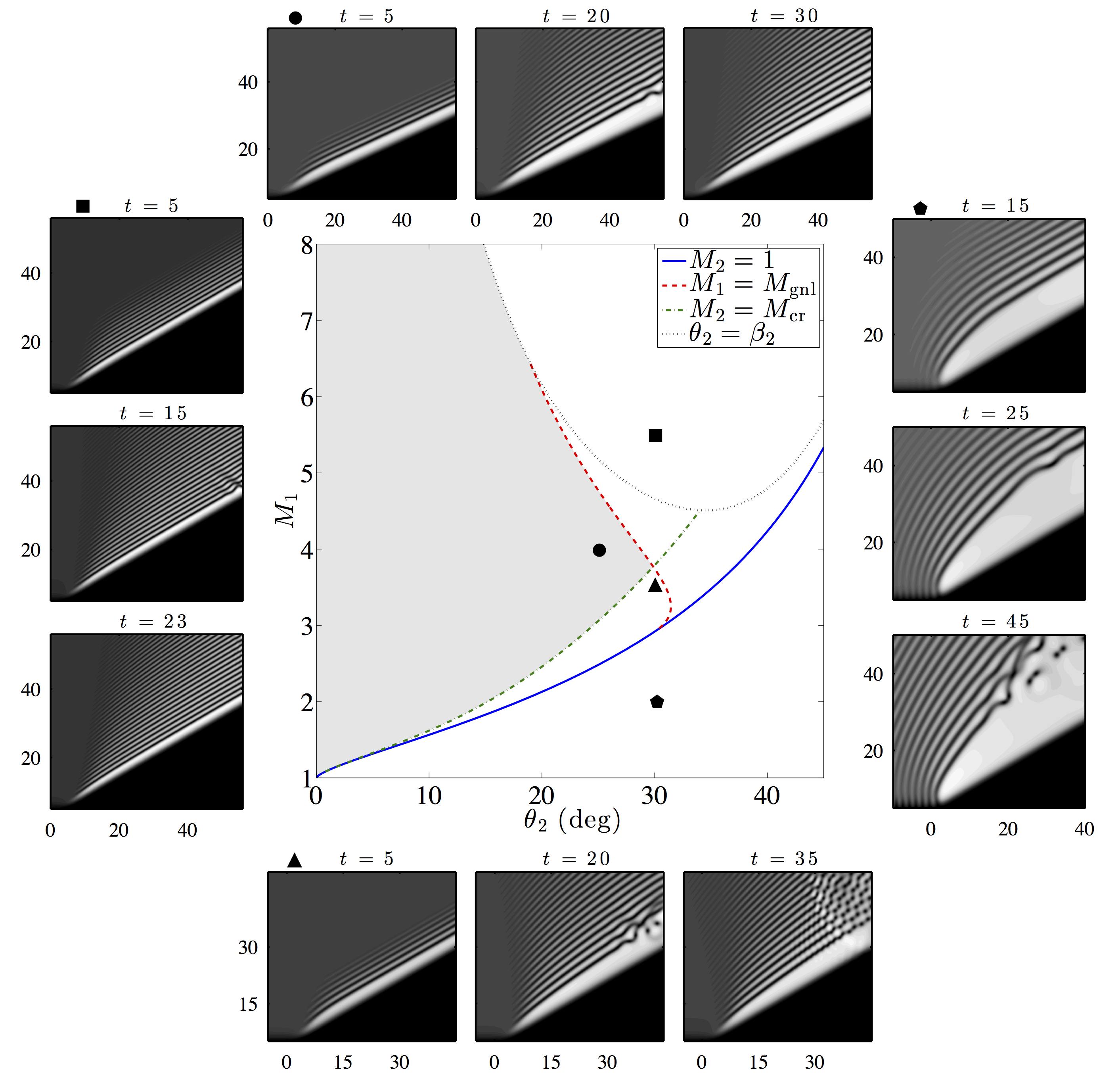
Figure 7. Phase diagram depicting the region of $(\theta_{2},M_{1})$ parameter space (gray) where oblique DSWs are causal $(M_{2}>1)$, admissible $(M_{1}<M_{\rm gnl})$, convectively unstable $(M_{2}>M_{\rm cr})$, and non-cavitating $(\theta_{2}<\beta_{2})$. Numerical simulations of flow past corner: –causal, admissible, convectively unstable, $M_{1}=4$, $\theta_{2}=25^{\circ}$; –causal, admissible, absolutely unstable, $M_{1}=3.5$, $\theta_{2}=30^{\circ}$; –not causal, $M_{1}=2$, $\theta_{2}=30^{\circ}$; –cavitation, $M_{1}=5.5$, $\theta_{2}=30^{\circ}$.

Although for certain parameters the oblique DSW may be causal and admissible, it is unstable. It is well-known that line dark solitons are unstable to long wavelength transverse perturbations [30]. As of yet, there is not a full analysis of DSW instability but because the oblique DSW exhibits a dark soliton edge, the dark soliton’s instability properties are effectively inherited by the DSW. The instability type, convective or absolute, depends on the Mach number $M$ of the background flow [26, 22]. If $M>M_{\rm cr}$, then any localized perturbation along an oblique dark soliton, considered at a fixed point, decays in time; i.e., the instability is “convected away” by the flow. When $M<M_{\rm cr}$, absolute instability, perturbations grow in time at any fixed point in space. The critical Mach number $M_{\rm cr}$ depends on the normalized dark soliton amplitude $0<\nu=a_{\rm s}/\bar{\rho}\leq 1$ and exhibits the bounds $1<M_{\rm cr}(\nu)\lessapprox 1.4374$ and the small amplitude asymptotics $M_{\rm cr}=1+\frac{2}{9}\nu^{4}+\mathcal{O}(\nu^{6})$ [22]. For larger $\nu$, $M_{\rm cr}(\nu)$ must be computed. The Mach number of the oblique DSW flow adjacent to the soliton edge is $M_{2}$. Therefore, we predict a convectively unstable oblique DSW when $M_{2}>M_{\rm cr}$ and an absolutely unstable oblique DSW otherwise.

The four conditions for a causal ($M_{2}>1$), admissible ($M_{1}<M_{\rm gnl}$), convectively unstable ($M_{2}>M_{\rm cr}$), and non-cavitating ($\theta_{2}<\beta_{2}$) (valid) oblique DSW, are depicted in the phase diagram of fig. 7. Our oblique DSW construction is valid across a range of upstream Mach numbers $M_{1}$ and downstream flow angles $\theta_{2}$. We find a maximum valid flow angle of $\theta_{2}\approx 30^{\circ}$ where $M_{1}\approx 3.8$.

Figure 7 shows the time evolution, in the reference frame of the corner, of four distinct regimes of the phase diagram. The valid region is represented by the simulation annotated with a filled circle where an oblique DSW develops; the transverse instability is apparent, but ultimately convects away from the corner, leaving two distinct angles that enclose the oscillatory oblique DSW. The simulation annotated by a filled triangle develops in a similar fashion, but due to absolute instability, waves invade the oblique DSW, migrating down to the corner. A more violent instability occurs for acausal parameter choices, represented by the filled pentagon. The downstream flow is predicted to be subsonic and is accompanied by the unsteady, forward propagation of dispersive waves. Absolute instability corresponds to the breakup of the wavetrain into vortices that eventually overwhelm the flow. We also include a simulation of the cavitating regime, annotated by the filled square, where an oblique DSW forms that is effectively “attached” to the corner. In the hypersonic regime, cavitating DSWs were shown to no longer exhibit a dark soliton edge [12]. Rather, the edge is described by a non-modulated periodic wavetrain adjacent to a modulated region whose envelope decays to the harmonic wave edge.

While the simulations depicted in fig. 7 show the distinction between convective and absolute instability, longer time DSW stability can be more complicated. In the case of convective instability, a large number of vortices are generated and are initially convected away from the corner. However, these vortices can reflect off of the boundary and interact with the DSW. This results in wave generation that can eventually propagate throughout the DSW, effectively rendering it unstable for long enough evolution time. One way to avoid this effect is to terminate the ramp at some finite distance away from the corner so that the generated vortices do not reflect off the boundary. This is what was done for the example identified by the filled circle in fig. 7 where the ramp was terminated at $x=55$.

5. Discussion and conclusion

We have constructed the theory of steady, oblique, two-dimensional spatial dispersive shock waves (DSWs) in the framework of the defocusing nonlinear Schrödinger (NLS) equation. This problem is of fundamental interest as a dispersive counterpart of the classical gas dynamics problem but also is motivated by actual physical applications in superfluid dynamics and nonlinear optics where the NLS equation is an accurate mathematical model. The prototypical flow past corner problem has been considered that elucidates the key properties of steady oblique DSWs. The main development of the paper is that the theory has been constructed for general supersonic flows, without additional simplifying assumptions (small corner angle or highly supersonic oncoming flow) enabling one to asymptotically reduce the description of steady oblique DSWs to solving a Riemann problem for an integrable equation: either KdV or (1+1)D NLS [15, 16, 12]. In contrast, the full (2+0)D defocusing NLS equation is not integrable and also exhibits a number of qualitative, structural differences compared to the above asymptotic (1+1)D models. Thus, the previously existing theory of steady oblique DSWs required significant development.

In this paper, we have employed the simple wave DSW fitting method [7, 10], which is based on Whitham nonlinear modulation theory [38] and is applicable to non-integrable systems of dispersive hydrodynamics. We determine the definitive characteristics of a steady oblique DSW: its locus and the bounding angles. We have identified the range of input parameters (the Mach number of the upstream flow $M_{1}$ and the corner angle $\theta_{2}$) for which the constructed simple-wave modulation description is valid. The main restrictions include causality inequalities and the condition of genuine nonlinearity of the modulation equations. An additional restriction of the simple wave DSW theory specific to the defocusing (2+0)D NLS equation is the requirement of the absence of DSW cavitation. For sufficiently large flow deflection angles, an additional wave structure exhibiting points of zero density in the region adjacent to the corner can occur.

Importantly, admissible stationary oblique DSWs exhibit instability, either convective or absolute. The convectively unstable DSWs are effectively stable in the laboratory reference frame [26, 21, 22] and so can be manifested in an experiment, although a full DSW stability theory has not yet been developed. Convective instability is a unique property of steady oblique 2D DSWs which contrasts them to their unsteady 1D counterparts, which are always stable. When the Mach number of the downstream flow is smaller than a critical value $M_{cr}$, the convective instability is replaced by absolute instability and further, by a non-causal, subsonic regime. The boundaries of the regions in the $\theta_{2},M_{1}$ phase plane corresponding to the various oblique DSW generation regimes have been identified numerically.

The constructed theory of stationary oblique DSWs suggests several directions of further research. A natural next step would be the generalization of the developed theory to more complicated geometries such as supersonic NLS flow past an airfoil exhibiting two types of oblique DSWs with contrasting asymptotic behaviors (see [16, 12] for the descriptions in the frameworks of integrable asymptotic reductions). The development of the full theory of oblique DSW stability remains an important open problem. Yet another closely related open problem is the description of transonic dispersive flows. Finally, due to the common structure of the dispersionless equations, the analysis performed here can be generalized to other Eulerian dispersive hydrodynamic systems [18, 10] such as shallow water waves.

Appendix A Simple Wave ODEs

In this appendix, we derive the simple wave ODE eq. 49 utilizing the parametric representation eqs. 30 and 31 of the linear dispersion relation.

A.1. Harmonic Edge

The zero amplitude modulation equations are the dispersionless equations eq. 39 for the averaged variables $(\overline{\rho},\overline{\mathbf{u}})$ or, equivalently $(\overline{\rho},\overline{\mu},\overline{\theta})$, coupled to the conservation of waves eq. 38, where $\omega$ corresponds to the linear dispersion relation eq. 27. For a simple wave, the relations eq. 45 and eq. 47 hold, determining $\overline{\rho}=\overline{\rho}(\overline{\mu})$ and $\overline{\theta}=\overline{\theta}(\overline{\mu})$. This leaves two modulation equations

(69) $$\begin{split}A\begin{bmatrix}\overline{\mu}\\ \varphi\end{bmatrix}_{y}+&B\begin{bmatrix}\overline{\mu}\\ \varphi\end{bmatrix}_{x}=0,\\ A=\begin{bmatrix}1&0\\ q_{\overline{\mu}}\sin\varphi&q_{\varphi}\sin\varphi+q\cos\varphi\end{bmatrix},\quad&B=\begin{bmatrix}\lambda_{+}&0\\ q_{\overline{\mu}}\cos\varphi&q_{\varphi}\cos\varphi-q\sin\varphi\end{bmatrix},\end{split}$$

where we have used the parametric representation eq. 30, eq. 31 with parameter $\varphi$ for the linear dispersion relation. This system has two characteristic speeds: $\lambda_{+}$, the dispersionless characteristic, and

(70) $$\frac{q_{\varphi}\cos\varphi-q\sin\varphi}{q_{\varphi}\sin\varphi+q\cos\varphi}=\frac{\omega_{\varphi}}{k_{\varphi}}=\omega_{k},$$

the group velocity of linear waves. A simple wave along the $\lambda_{+}$ characteristic corresponds to the Prandtl-Meyer expansion fan eq. 42 in dispersionless dynamics. For the DSW, we seek the simple wave along the $\omega_{k}$ characteristic. The goal is to determine the appropriate wavenumber $k$ at which to evaluate the group velocity given the Riemann initial data eq. 15. The left eigenvector

(71) $$l^{T}=\begin{bmatrix}q_{\overline{\mu}}(\cos\varphi-\omega_{k}\sin\varphi)&\omega_{k}-\lambda_{+}\end{bmatrix},$$

satisfies the relation $l^{T}B=\omega_{k}l^{T}A$. Applying $l^{T}$ to equation eq. 69 results in the characteristic form

(72) $$l^{T}A\begin{bmatrix}\mathrm{d}\overline{\mu}\\ \mathrm{d}\varphi\end{bmatrix}=0.$$

We seek a solution in the form $\varphi=\varphi(\overline{\mu})$, yielding the simple wave ODE

(73) $$\begin{split}\frac{\mathrm{d}\varphi}{\mathrm{d}\overline{\mu}}&=\frac{q_{\overline{\mu}}(\cos\varphi-\lambda_{+}\sin\varphi)}{\sin\varphi(\lambda_{+}q_{\varphi}+q)+\cos\varphi(\lambda_{+}q-q_{\varphi})},\end{split}$$

that simplifies to the ODE in eq. 51. The zero wavenumber condition at the soliton edge $k(\varphi,\mu_{2})=0=\omega(\varphi,\mu_{2})$ corresponds to $q(\varphi,\mu_{2})=0$ and the initial data

(74) $$\varphi(\mu_{2})=\overline{\theta}(\mu_{2})+\mu_{2}.$$

A.2. Soliton Edge

For the soliton edge, we utilize the conjugate dispersion relation eq. 52, defined parametrically according to

(75) $$\begin{split}\tilde{k}&=\tilde{q}\sin\tilde{\varphi},\quad\tilde{\omega}=\tilde{q}\cos\tilde{\varphi},\quad\tilde{q}=2\overline{\rho}^{1/2}\left(1-\frac{\sin^{2}(\tilde{\varphi}-\overline{\theta})}{\sin^{2}\overline{\mu}}\right)^{1/2}\end{split}$$

A similar calculation to that in the previous section with $q\to\tilde{q}$, $\varphi\to\tilde{\varphi}$ leads to the same simple wave ODE

(76) $$\begin{split}\frac{\mathrm{d}\tilde{\varphi}}{\mathrm{d}\overline{\mu}}=\frac{\tilde{q}_{\overline{\mu}}(\cos\tilde{\varphi}-\lambda_{+}\sin\tilde{\varphi})}{\sin\tilde{\varphi}(\lambda_{+}\tilde{q}_{\tilde{\varphi}}+\tilde{q})+\cos\tilde{\varphi}(\lambda_{+}\tilde{q}-\tilde{q}_{\tilde{\varphi}})},\end{split}$$

that can be simplified to eq. eq. 55. The zero amplitude condition $\tilde{k}(\tilde{\varphi},\mu_{1})=0=\tilde{\omega}(\tilde{\varphi},\mu_{1})$ at the harmonic edge provides the initial condition $\tilde{q}(\tilde{\varphi},\mu_{1})=0$ or

(77) $$\tilde{\varphi}(\mu_{1})=\overline{\theta}(\mu_{1})+\mu_{1}=\mu_{1}.$$

References

- [1] M. J. Ablowitz and D. E. Baldwin, Interactions and asymptotics of dispersive shock waves – Korteweg-de Vries equation, Phys. Lett. A, 377 (2013), pp. 555–559.
- [2] M. J. Ablowitz, A. Demirci, and Y.-P. Ma, Dispersive shock waves in the Kadomtsev-Petviashvili and two dimensional Benjamin-Ono equations, Physica D, 333 (2016), pp. 84–98.
- [3] R. W. Boyd, Nonlinear Optics, Academic Press, Cambridge, MA, 2013.
- [4] R. Courant and K. O. Friedrichs, Supersonic Flow and Shock Waves, Springer-Verlag, New York, 1948.
- [5] B. Dubrovin, T. Grave, and C. Klein, On critical behaviour in generalized Kadomtsev-Petviashvili equations, Physica D, 333 (2016), p. 157–170.
- [6] Z. Dutton, M. Budde, C. Slowe, and L. V. Hau, Observation of quantum shock waves created with ultra-compressed slow light pulses in a Bose-Einstein condensate, Science, 293 (2001), p. 663.
- [7] G. A. El, Resolution of a shock in hyperbolic systems modified by weak dispersion, Chaos, 15 (2005), 037103.
- [8] G. A. El, A. Gammal, and A. M. Kamchatnov, Oblique dark solitons in supersonic flow of a Bose-Einstein condensate, Phys. Rev. Lett., 97 (2006), 180405.
- [9] G. A. El, Y. G. Gladush, and A. M. Kamchatnov, Two-dimensional periodic waves in supersonic flow of a Bose-Einstein condensate, J. Phys. A, 40 (2007), pp. 611–619.
- [10] G. A. El and M. A. Hoefer, Dispersive shock waves and modulation theory, Physica D, 333 (2016), pp. 11–65.
- [11] G. A. El and A. M. Kamchatnov, Spatial dispersive shock waves generated in supersonic flow of Bose-Einstein condensate past slender body, Phys. Lett. A, 350 (2006), pp. 192–196.
- [12] G. A. El, A. M. Kamchatnov, V. V. Khodorovskii, E. S. Annibale, and A. Gammal, Two-dimensional supersonic nonlinear Schrodinger flow past an extended obstacle, Phys. Rev. E, 80 (2009), 046317.
- [13] N. Ghofraniha, C. Conti, G. Ruocco, and S. Trillo, Shocks in nonlocal media, Phys. Rev. Lett., 99 (2007), 043903.
- [14] Y. G. Gladush, G. A. El, A. Gammal, and A. M. Kamchatnov, Radiation of linear waves in the stationary flow of a Bose-Einstein condensate past an obstacle, Phys. Rev. A, 75 (2007), 033619.
- [15] A. V. Gurevich, A. L. Krylov, V. V. Khodorovskii, and G. A. El, Supersonic flow past bodies in dispersive hydrodynamics, Sov. Phys. JETP, 81 (1995), pp. 87–96.
- [16] A. V. Gurevich, A. L. Krylov, V. V. Khodorovskii, and G. A. El, Supersonic flow past finite-length bodies in dispersive hydrodynamics, Sov. Phys. JETP, 82 (1996), pp. 709–718.
- [17] A. V. Gurevich and L. P. Pitaevskii, Nonstationary structure of a collisionless shock wave, Sov. Phys. JETP, 38 (1974), pp. 291–297. Translation from Russian of A. V. Gurevich and L. P. Pitaevskii, Zh. Eksp. Teor. Fiz. 65, 590-604 (1973).
- [18] M. A. Hoefer, Shock waves in dispersive Eulerian fluids, J. Nonl. Sci., 24 (2014), pp. 525–577.
- [19] M. A. Hoefer, M. J. Ablowitz, I. Coddington, E. A. Cornell, P. Engels, and V. Schweikhard, Dispersive and classical shock waves in Bose-Einstein condensates and gas dynamics, Phys. Rev. A, 74 (2006), 023623.
- [20] M. A. Hoefer, M. J. Ablowitz, and P. Engels, Piston dispersive shock wave problem, Phys. Rev. Lett., 100 (2008), 084504.
- [21] M. A. Hoefer and B. Ilan, Theory of two-dimensional oblique dispersive shock waves in supersonic flow of a superfluid, Phys. Rev. A, 80 (2009), 061601(R).
- [22] M. A. Hoefer and B. Ilan, Dark Solitons, Dispersive Shock Waves, and Transverse Instabilities, SIAM Mult. Mod. Sim., 10 (2012), pp. 306–341.
- [23] S. Jin, C. D. Levermore, and D. W. McLaughlin, The semiclassical limit of the defocusing NLS hierarchy, Comm. Pure Appl. Math., 52 (1999), pp. 613–654.
- [24] A. Kamchatnov and S. Korneev, Flow of a Bose-Einstein condensate in a quasi-one-dimensional channel under the action of a piston, JETP, 110 (2010), pp. 170–182.
- [25] A. Kamchatnov and S. Korneev, Condition for convective instability of dark solitons, Phys. Lett. A, 375 (2011), pp. 2577–2580.
- [26] A. M. Kamchatnov and L. P. Pitaevskii, Stabilization of solitons generated by a supersonic flow of Bose-Einstein condensate past an obstacle, Phys. Rev. Lett., 100 (2008), 160402.
- [27] Y. V. Kartashov and A. M. Kamchatnov, Two-dimensional dispersive shock waves in dissipative optical media, Opt. Lett., 38 (2013), p. 790.
- [28] C. Klein and K. Roidot, Numerical study of shock formation in the dispersionless Kadomtsev-Petviashvili equation and dispersive regularizations, Physica D, 265 (2013), pp. 1–25.
- [29] C. Klein, C. Sparber, and P. A. Markowich, Numerical study of oscillatory regimes in the Kadomtsev-Petviashvili equation, J. Nonlin. Sci., 17 (2007), pp. 429–470.
- [30] E. A. Kuznetsov and S. K. Turitsyn, Instability and collapse of solitons in media with a defocusing nonlinearity, Sov. Phys. JETP, 67 (1988), pp. 1583–1588.
- [31] P. D. Lax, Hyperbolic systems of conservation laws and the mathematical theory of shock waves, SIAM, Philadelphia, 1973.
- [32] P. D. Lax and C. D. Levermore, The small dispersion limit of the Korteweg-de Vries equation: 1-3, Comm. Pure Appl. Math., 36 (1983), pp. 253–290; 571–593; 809–830.
- [33] L. P. Pitaevskii and S. Stringari, Bose-Einstein condensation, Clarendon, Oxford, 2003.
- [34] T. P. Simula, P. Engels, I. Coddington, V. Schweikhard, E. A. Cornell, and R. J. Ballagh, Observations on sound propagation in rapidly rotating Bose-Einstein condensates, Phys. Rev. Lett., 94 (2005), 080404.
- [35] S. Venakides, Long time asymptotics of the Korteweg-de Vries equation, Trans. Amer. Math. Soc, 293 (1986), pp. 411–419.
- [36] W. Wan, S. Jia, and J. W. Fleischer, Dispersive superfluid-like shock waves in nonlinear optics, Nat. Phys., 3 (2007), pp. 46–51.
- [37] G. B. Whitham, Non-linear dispersive waves, Proc. Roy. Soc. Ser. A, 283 (1965), pp. 238–261.
- [38] G. B. Whitham, Linear and Nonlinear Waves, Wiley, New York, 1974.