IFJ PAN-IV-2016-19

Potential for optimizing Higgs boson CP measurement

in $H\to\tau\tau$ decay at LHC and ML techniques

R. Józefowicz^a,⋆, E. Richter-Was^b and Z. Was^c
a Open AI, San Francisco, CA, USA

^b Institute of Physics, Jagellonian University, Lojasiewicza 11, 30-348 Krakow, Poland

^c Institute of Nuclear Physics Polish Academy of Sciences , PL-31342 Krakow, Poland

ABSTRACT

We investigate potential for measuring CP state of the Higgs boson in the $H\to\tau\tau$ decay with consecutive $\tau$-lepton decays in channels: $\tau^{\pm}\to\rho^{\pm}\nu_{\tau}$ and $\tau^{\pm}\to a_{1}^{\pm}\nu_{\tau}$ combined. Subsequent decays $\rho^{\pm}\to\pi^{\pm}\pi^{0}$, $a_{1}^{\pm}\to\rho^{0}\pi^{\pm}$ and $\rho^{0}\to\pi^{+}\pi^{-}$ are taken into account. We will explore extensions of the method, where acoplanarity angle for the planes build on the visible decay products, $\pi^{\pm}\pi^{0}$ of $\tau^{\pm}\to\pi^{\pm}\pi^{0}\nu_{\tau}$, was used. The angle is sensitive to transverse spin correlations, thus to parity.

We show, that in the case of the cascade decays of $\tau\to a_{1}\nu$, information on the CP state of Higgs can be extracted from the acoplanarity angles as well. Because in the cascade decay $a_{1}^{\pm}\to\rho^{0}\pi^{\pm},\;\rho^{0}\to\pi^{+}\pi^{-}$ up to four planes can be defined, up to 16 distinct acoplanarity angles are available for $H\to\tau\tau\to a_{1}^{+}a_{1}^{-}\nu\nu$ decays. These acoplanarities carry in part supplementary but also correlated information. It is thus cumbersome to evaluate an overall sensitivity.

We investigate sensitivity potential of such analysis, by developing and implementing model in the Machine Learning (ML) techniques. We quantify possible improvements when multi-dimensional phase-space of outgoing decay products directions is used, instead of 1-dimensional projections i.e. the acoplanarity angles.

We do not take into account ambiguities resulting from detector uncertainties or background contamination, we concentrate on usefulness of ML methods and $\tau\to 3\pi\nu$ decays for Higgs boson parity measurement.

IFJ PAN-IV-2016-19

August 2016

^⋆ Work performed while at Google, 75 Ninth Avenue, New York, NY 10011, USA

1 Introduction

The discovery of the Higgs boson by LHC experiments [1, 2] was followed by the measurements of its basic quantum numbers, such as spin [3, 4], mass [5], couplings to fermions and bosons [6] and parity [4, 7]. In particular, measurement of the CP state was possible, but so far only in the diboson decays. The exploration whether the discovered Higgs boson is a pure CP-even state in its coupling to fermions, or if admixture of the odd state is present, is of prime interest for the LHC physics program of the next years. If the CP-odd component is detected it would be an evidence of the new physics: the non-standard CP-violation. One way to probe parity of the $H$ couplings to fermions is discussed in the literature since decades [8]. It relies on the measurement of transverse spin correlations in the $H\to\tau\tau$ decay.

The loss of neutrinos for detection, and detector precision was limiting the original method of [8]. The possible way out, was found in [9]. It relied on measurement of spin correlations between visible decay product of $\tau$’s, more precisely the $\pi^{\pm}\pi^{0}$ from the dominant $\tau$ decay channel: $\tau^{\pm}\to\pi^{\pm}\pi^{0}\nu_{\tau}$. This decay channel of single intermediate spin one state is saturated by $\rho^{\pm}$. It was relatively easy to define corresponding observable: acoplanarity angle of two planes (defined in $\rho^{+}\rho^{-}$ pair rest frame), spanned respectively on $\pi^{+}\pi^{0}$ and $\pi^{-}\pi^{0}$. To achieve sensitivity to CP state, events had to be split into two groups; relative sign of energy differences for $\pi^{\pm}$ and $\pi^{0}$ for each of the two pairs was used to separate events. The method presented in [9], does not need much adaptation for the LHC measurements, see eg. [10]. Similarly as in the Linear Collider case, there is no need to reconstruct $\tau$ lepton rest-frames, it was enough to reconstruct rest frame of the $\rho^{\pm}\ \rho^{\mp}$ pair.

A prospect to extend measurements to other $\tau$ decay modes is tempting. The $\tau$ lepton decays into variety of channels. More than 20 different decay channels have been observed. In the present paper we will study extension of the acoplanarity angle method to other sizable $\tau$ decay channel, namely $\tau^{\pm}\to(3\pi)^{\pm}\nu$.

Started in Ref. [11] effort to exploit all 1-prong $\tau$ decay modes lead to several publications [12, 13, 14, 15, 16]. An idea that position of decay $\tau$ vertex could be used as a backbone of the measurement was promising substantial gain in sensitivity, certainly better than if vertex reconstruction was assumed to be at the measurability limit only [17]. Use of the decay vertex is expected to be particularly promising in case of 3-prong $\tau$ decays, with already achieved performance of tracking and vertexing of LHC experiments [18, 19, 20].

In the following study, let us concentrate, on measurement sensitivity which can be achieved for $H\to\tau\tau$ data without exploitation of $\tau$ decay vertex. Instead we will explore in a greater detail effects due to spin correlations in cascade $\tau$ decays. In Table 1 we show branching ratios for specific modes discussed in this analysis. Inclusion of $a_{1}^{\pm}\to\rho^{0}\pi^{\pm},\ \rho^{0}\to\pi^{+}\pi^{-}$ or $a_{1}^{\pm}\to 2\pi^{0}\ \pi^{\pm}$ increases the available fraction of $H\to\tau\tau$ decay rate from 6.5 to 19.2 %. For the analysis discussed here we will consider either $\tau$ decay to 3 charged $\pi$ or $\tau$ decay to $\pi^{\pm}\ \pi^{0}$ with intermediate $\rho^{\pm}$ resonance. That results in an increase of statistical sample by a factor of nearly two, from 6.5 to 11.9 %.

Our paper is organized as follows. In Section 2 we demonstrate that indeed acoplanarity angles can be defined in case of $\tau^{\pm}\to a_{1}^{\pm}\nu$ decays and if events are split into appropriate groups, sensitivity to CP parity of the Higgs boson can be achieved for this 1-dimensional variables. Because several such angles can be defined for the $\tau$ decays into more than two scalars, we demonstrate in Section 3, that all resulting observables, if combined together using methods of Machine Learning (ML), like Deep Learning Neural Network, can improve sensitivity. We discuss also, how information has to be prepared for Neural Network to assure sensitivity. Summary, Section 4, closes the paper.

2 The 1-dimensional analyzes

Let us discuss now in more details observables for the three cases: (i) $H\to\tau\ \tau\to\rho^{\pm}\ \rho^{\mp}\ 2\ \nu$, (ii) $H\to\tau\ \tau\to\rho^{\pm}\ a_{1}^{\mp}\ 2\ \nu$ and (iii) $H\to\tau\ \tau\to a_{1}^{\pm}\ a_{1}^{\mp}\ 2\ \nu$. The rates for those configurations with respect to the total $H\to\tau\tau$ rate are 6.5%, 4.6% and 0.8% respectively, see Table 1. The relatively well established strategy for CP measurement exists for the configuration (i). One can significantly increase available for analysis statistics if also (ii) and (iii) configurations are used. At this moment, we have no intention to explore a $\pi^{0}\pi^{0}\pi^{\pm}$ tau decay, even though from the physics point of view it would be straightforward and available sample of events would again increase significantly, see Table 1. This case, because of experimental context requires evaluation if 2$\pi^{0}$’s can be resolved.

The 1-dimensional analysis, as discussed in this section, will rely on building 1-dimensional observable, or a few of them, sensitive to the CP nature of the Higgs boson. Below, we propose those observables, but without an attempt to quantify possible sensitivity of the experimental analysis, especially consequences of existing correlations between variables.

We extend definition of an acoplanarity angle introduced for the $\tau\to\pi^{\pm}\pi^{0}\nu$ decay to a few more available for $\tau^{\pm}\to a_{1}^{\pm}\nu$ decay and extend also definition of variable which can be used to split events into groups necessary for discrimination between different CP states. The subtle effect of the CP-even vs CP-odd nature manifests itself in these angular distributions of $\tau$ decay products: the acoplanarity angle(s) $\varphi^{*}_{i,k}$ between planes defined by the visible decay products in the hadronic cascades starting from the $\tau$ leptons. The sub-scrips $i,k$ are used to index elementary decays of the cascades and the corresponding decay planes. Introduction of indices is convenient if there are more than two visible decay products of the $\tau^{\pm}$.

For numerical studies, we use Monte Carlo events of the SM, 125 GeV mass, Higgs boson, produced in pp collision at 13 TeV centre-of-mass energy, generated with Pythia 8.2 and with spin correlations simulated using TauSpinner [10] package. For $\tau$ lepton decays we use Tauolapp library [21]. All spin and parity effects are implemented with the help of TauSpinner weight $wt^{CP}$. That is why, samples prepared for CP even or odd Higgs are correlated.

In our studies, to emulate partly detector conditions, a minimal set of cuts is used. We require that the transverse momenta of the visible decay products combined, for each $\tau$, is bigger than 20 GeV. It is also required that transverse momentum of each $\pi^{\pm}$ is bigger than 1 GeV.

2.1 The $H\to\tau\ \tau\to\rho^{\pm}\ \rho^{\mp}\ 2\ \nu$ case

This final state configuration contributes about 6.5% of all $H\to\tau\ \tau$ decays. The method of using the acoplanarity $\varphi^{*}_{\rho^{+}\rho^{-}}$ of the $\rho^{\pm}$ decay planes in $\rho^{\pm}-\rho^{\mp}$ centre-off-mass system as sensitive observable, proposed in [9], has been so far considered as the most promising one. This method requires that the track from the charged $\pi^{\pm}$ and a cluster from $\pi^{0}$ can be separated, which is now well within experimental reach of the LHC detectors [18, 19].

The sample is split into two sub-groups, with the help of the sign for the differences of $\pi^{\pm}$ and $\pi^{0}$ energies. For each $\tau^{\pm}$ in the pair, we define

$$y_{\rho}^{\pm}=\frac{E^{\pi^{\pm}}-E^{\pi^{0}}}{E^{\pi^{\pm}}+E^{\pi^{0}}}$$ (1)

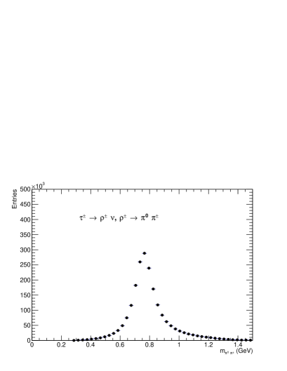
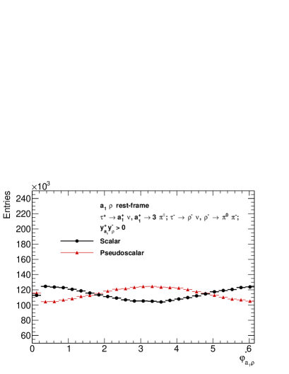
and we group events into two categories depending on the sign of the product $y_{\rho}^{+}y_{\rho}^{-}$. The $E^{\pi^{\pm}}$ and $E^{\pi^{0}}$ can be defined in the $\rho^{+}\rho^{-}$ rest frame or in laboratory frame, with no sizable difference of the sensitivity. In each group, acoplanarity angle $\varphi^{*}_{\rho^{+},\rho^{-}}$ shows nice sinusoidal shape which is shifted by $180^{\circ}$ between the cases of scalar and pseudo-scalar Higgs. Note that if the shift was present but was smaller than $180^{\circ}$, the size of that shift would measure the mixing between two CP states of the Higgs boson. We will return to this point in Subsection 2.4. Fig. 1 shows overlaid distributions for of the scalar (black) and pseudo-scalar (red) models, for each group of events separated by the sign of the product $y_{\rho}^{+}y_{\rho}^{-}$. On the Fig. 1 we show also line shape of the $\pi^{\pm}\pi^{0}$ mass, for system originating from the same $\tau$.

2.2 The $H\to\tau\ \tau\to a_{1}^{\pm}\ \rho^{\mp}\ 2\ \nu$ case

Decay mode	Cascade decay	$\tau$ BR.	Cumul. $H\to\tau\tau$ frac.	Used for analysis
$\tau^{\pm}\to\rho^{\pm}\nu$	$\rho^{\pm}\to\pi^{0}\ \pi^{\mp}$	25.5%	6.5%	Yes
$\tau^{\pm}\to a_{1}^{\pm}\nu$	$a_{1}^{\pm}\to\rho^{0}\pi^{\mp},\ \rho^{0}\to\pi^{+}\pi^{-}$	9.0%	11.9%	Yes
	$a_{1}^{\pm}\to 2\pi^{0}\ \pi^{\mp}$	9.3%	19.2%	No

Table 1: Branching ratios of the $\tau$ lepton decay modes [22], and resulting, cumulated fraction of $H\to\tau\tau$ events available for parity analysis.

Figure 1: Acoplanarity angle $\varphi^{*}_{\rho\rho}$ of oriented half decay plane for the decay products of $\rho^{+}$ and $\rho^{-}$. Events are grouped by the sign of $y_{\rho}^{+}y_{\rho}^{-}$. Invariant mass of the $\rho^{\pm}\to\pi^{+}\pi^{-}$ system (bottom) is also shown.

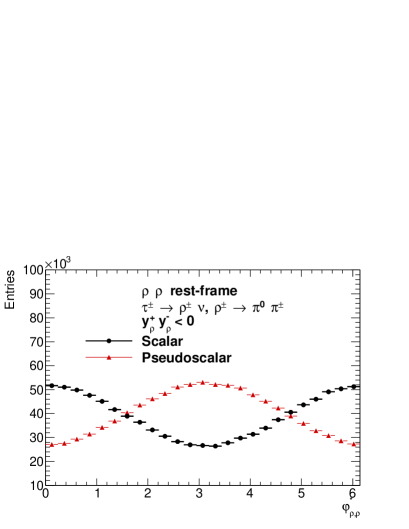
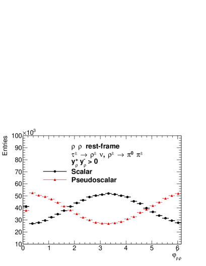
This final state configuration contribute about 4.6% of all $H\to\tau\ \tau$ decays. Let us extend the method explained in the previous sub-section to a new case, where there are two possibilities for the $a_{1}$ system decay plane definition. One can take the decay products of primary resonance $a_{1}^{\pm}$, or of secondary resonance $\rho^{0}$ originating from $\tau^{\pm}$ decays. Also, in case of $a_{1}^{\pm}\to 3\pi^{\pm}$ decay, we do not know which combinations of $\pi^{+}\pi^{-}$ form the intermediate $\rho^{0}$ resonance, for each event we take into account both combinations. Counting possible pairing, we finally construct 4 planes, thus 4 distinct acoplanarities with the plane of $\rho^{\mp}$, from the other $\tau$, decay. We could use reconstructed invariant masses, to decide which of the two $\pi^{+}\pi^{-}$ pairs is closer to the $\rho^{0}$ peak, and choose the corresponding acoplanarities only, but it was not straightforward to evaluate the impact on optimalization.

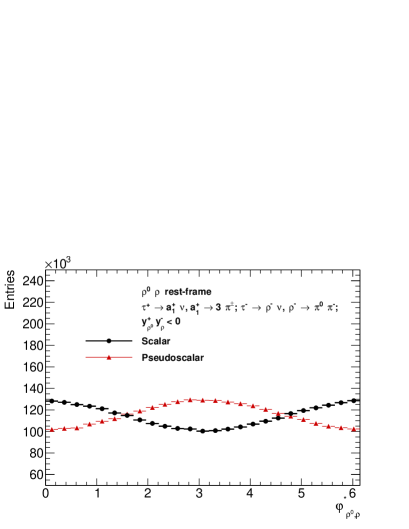
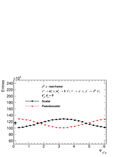
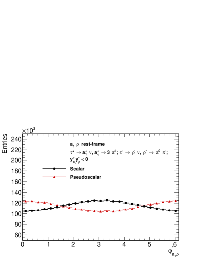
As in the previous case of Fig. 1, the discriminating shapes of the acoplanarity angles between scalar and pseudo-scalar CP states appear only if the samples are split into sub categories. In case of the $\tau^{\pm}\to a_{1}^{\pm}\nu$ decay we calculate $y_{a_{1}}^{\pm}$ and $y_{\rho^{0}}^{\pm}$

$$y_{\rho^{0}}^{\pm}=\frac{E^{\pi^{+}}-E^{\pi^{-}}}{E^{\pi^{+}}+E^{\pi^{-}}},\ \ \ \ y_{a_{1}}^{\pm}=\frac{E^{\rho^{0}}-E^{\pi^{\pm}}}{E^{\rho^{0}}+E^{\pi^{\pm}}}-\frac{m^{2}_{a_{1}}-m^{2}_{\pi^{\pm}}+m^{2}_{\rho^{0}}}{2m^{2}_{a_{1}}}$$ (2)

In this case we take into account in $y_{a_{1}}^{\pm}$ definition, that masses of $\rho^{0}$ and $\pi^{\pm}$ are substantially different. The sign of the product $y_{a_{1}}^{\pm}y_{\rho}^{\mp}$ or respectively $y_{\rho^{0}}^{\pm}y_{\rho}^{\mp}$ is used to split events into two separate categories, which are almost equally populated. The $m_{a_{1}}$ and $m_{\rho^{0}}$ denote respectively the invariant mass of $(3\pi)^{\pm}$ system and $(2\pi)$ system which we assume to form $a_{1}$ and $\rho^{0}$.

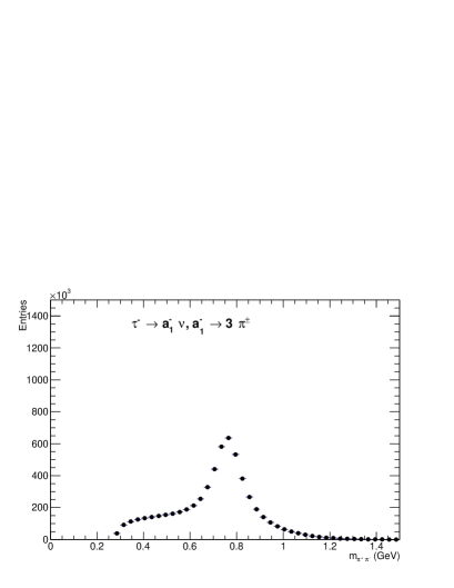
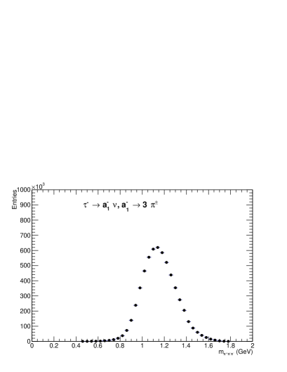
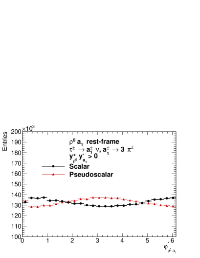
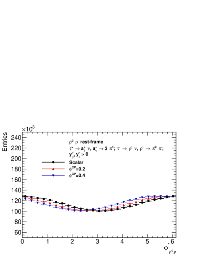
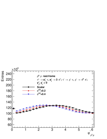
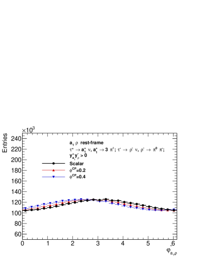
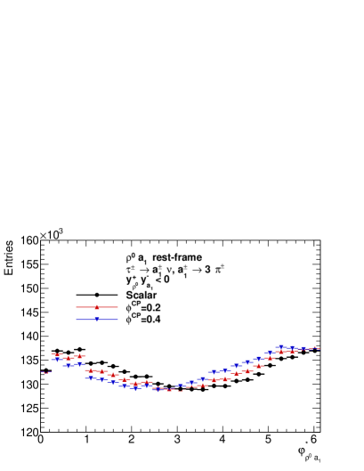
Fig. 3 shows overlaid shapes of the scalar (black) and pseudo-scalar (red) models. For each acoplanarity angle events are split into two groups, to make this observable CP sensitive. The amplitude of modulation is smaller than in previously discussed case, as the information on the CP state is now dissipated in the cascade decay of one $\tau$ lepton. Also it is smeared due to the possible wrong pairing for the $\pi^{+}\pi^{-}$ to form $\rho^{0}$ resonance. To illustrate effect of this wrong pairing, an invariant masses of the $\pi^{+}\pi^{-}$ and $\pi^{+}\pi^{-}\pi^{+}$ systems are also shown in Fig. 3. In total, four acoplanarity angles can be constructed. They all have quite similar sinusoidal shapes and carry CP information. They are correlated and their CP distinctive powers are not independent. That is why we do not quantify sensitivity in the scope of 1-dimensional histograms-observables. It was important to demonstrate that sensitivity is indeed present, and that acoplanarity angles are again good candidate for the definition of 1-dimensional observables. Note that for some plots of $\varphi^{*}_{i,k}$ it looks as if scalar/pseudo-scalar contributions were accidentally interchanged, it is the consequence of more complex nature of the 3$\pi$ decays.

Figure 2: Invariant mass of the $(3\pi)^{\pm}$ and $\pi^{+}\pi^{-}$ systems in case of one $\tau^{\pm}\to a_{1}^{\pm}\nu\to(3\pi)^{\pm}\nu$ decays.

Figure 3: Acoplanarity angles of oriented half decay planes: $\varphi^{*}_{\rho^{0}\rho}$ (top), $\varphi^{*}_{{a_{1}}\rho}$ (bottom), for events grouped by the sign of $y_{\rho^{0}}^{+}y_{\rho}^{-}$ and $y_{a_{1}}^{+}y_{\rho}^{-}$ respectively.

2.3 The $H\to\tau\ \tau\to a_{1}^{\pm}\ a_{1}^{\mp}\ 2\ \nu$ case

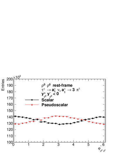
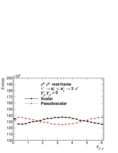
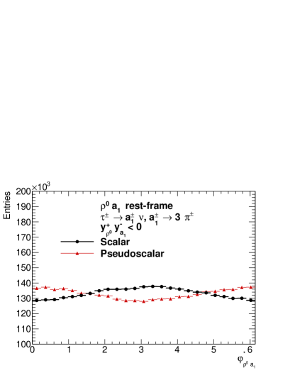
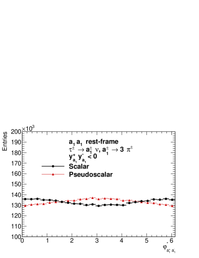
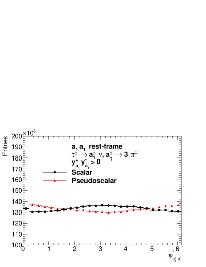
This final state contribute about 0.8% of all $H\to\tau\tau$ decays. We extend here the previously explained method to case with even more combinations of decay planes: $(a_{1}^{\pm},a_{1}^{\mp})$, $(a_{1}^{\pm},\rho^{0})$, $(\rho^{0},a_{1}^{\mp})$ and $(\rho^{0},\rho^{0})$. In total 16 distinct acoplanarity angles can be defined. For each acoplanarity angle, separation into two categories, depending on the sign of $y_{a_{1}}^{\pm}y_{a_{1}}^{\mp}$, $y_{a_{1}}^{\pm}y_{\rho^{0}}^{\mp}$, $y_{\rho^{0}}^{\pm}y_{a_{1}}^{\mp}$ and $y_{\rho^{0}}^{\pm}y_{\rho^{0}}^{\mp}$ products respectively is performed. Those variables are calculated as in Eqs. (1) and (2). In this case also, it was possible to achieve almost equal population of events separated by the sign of $y^{+}y^{-}$, and for each of 16 acoplanarity angles.

In the case of $a_{1}^{\pm}\to 3\pi^{\pm}$, a priori, we do not know which combinations of $\pi^{+}\pi^{-}$ formed the $\rho^{0}$ resonance: we take therefore into account all possible pairing of $\pi^{+}\pi^{-}$ in each $\tau$ decay. These four invariant masses respectively of two possible pairs of $\pi^{+}\pi^{-}$ forming $\rho^{0}$ defined for each of the two $\tau$’s, can be helpful again for sensitivity optimalization.

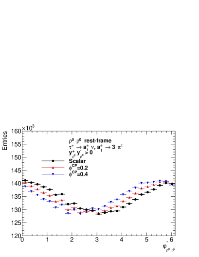
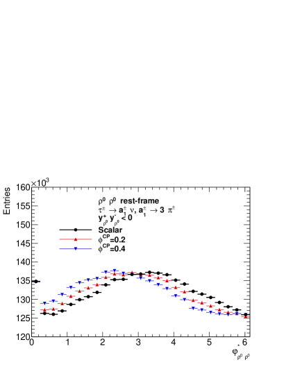
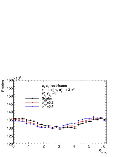
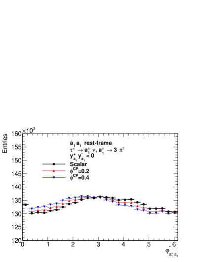
Fig. 4 shows overlaid shapes of the acoplanarity angles distributions for scalar (black) and pseudo-scalar (red) Higgs, for positive and negative products of $y_{\rho^{0}}^{+}y_{\rho^{0}}^{-}$, $y_{a_{1}}^{+}y_{\rho^{0}}^{-}$, $y_{\rho^{0}}^{+}y_{a_{1}}^{-}$, $y_{a_{1}}^{+}y_{a_{1}}^{-}$, given by formulae (1) and (2). The amplitude of modulation is smaller than in both previously discussed cases, as the information on the CP state is now dissipated in the cascade decays of both $\tau$ leptons. Also it is smeared due to two possible pairing of the $\pi^{+}\pi^{-}$ to form $\rho^{0}$ resonance. On the other hand, 16 correlated 1-dimension distributions are available.

Figure 4: Acoplanarity angles of oriented half decay planes: $\varphi^{*}_{\rho^{0}\rho^{0}}$ (top), $\varphi^{*}_{a_{1}\rho^{0}}$ (middle) and $\varphi^{*}_{a_{1}a_{1}}$ (bottom), for events grouped by the sign of $y_{\rho^{0}}^{+}y_{\rho^{0}}^{-}$, $y_{a_{1}}^{+}y_{\rho^{0}}^{-}$ and $y_{a_{1}}^{+}y_{a_{1}}^{-}$.

2.4 Case of CP mixing

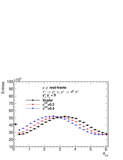
So far, we have compared distributions of the acoplanarity angles for pure scalar and pseudo-scalar CP states. For the mixed scalar-pseudo-scalar case, the general Higgs boson Yukawa coupling to the $\tau$ lepton

$$\bar{\tau}(a+ib\gamma_{5})\tau,$$ (3)

can be reparametrized with scalar-pseudo-scalar mixing angle $\phi^{CP}$, as in [23]

$$\frac{1}{\cal N}\bar{\tau}(\cos\phi^{CP}+i\ \sin\phi^{CP}\ \gamma_{5})\tau.$$ (4)

The mixed parity state is simulated by corresponding weight $wt^{CP}$ calculated with TauSpinner package [10]. Figures 6 -  7 show shift in the acoplanarity distributions for cases of mixing angle $\phi^{CP}$ = 0.0, 0.2 and 0.4 and three configurations of the $\tau$’s decay modes discussed above. Shift in all distributions of acoplanarity angle of $\Delta\varphi^{*}=2\phi^{CP}$ is observed, as presented in [23] already.

Figure 5: Acoplanarity angles of oriented half decay plane, $\varphi^{*}_{\rho\rho}$, for events grouped by the sign of $y_{\rho}^{+}y_{\rho}^{-}$. Shown are distributions for three values of mixing angle $\alpha_{CP}$ = 0.0 (scalar), 0.2 and 0.4.

Figure 6: Acoplanarity angles of oriented half decay planes: $\varphi^{*}_{\rho^{0}\rho}$ (top), $\varphi^{*}_{a_{1}\rho}$ (bottom), for events grouped by the sign of $y_{\rho^{0}}^{+}y_{\rho}^{-}$ and $y_{a_{1}}^{+}y_{\rho}^{-}$ respectively. Shown are distributions for three values of mixing angle $\phi^{CP}$ = 0.0 (scalar), 0.2 and 0.4.

Figure 7: Acoplanarity angles of oriented half decay planes: $\varphi^{*}_{\rho^{0}\rho^{0}}$ (top), $\varphi^{*}_{a_{1}\rho^{0}}$ (middle) and $\varphi^{*}_{a_{1}a_{1}}$ (bottom), for events grouped by the sign of $y_{\rho^{0}}^{+}y_{\rho^{0}}^{-}$, $y_{a_{1}}^{+}y_{\rho^{0}}^{-}$ and $y_{a_{1}}^{+}y_{a_{1}}^{-}$ respectively. Shown are distributions for three values of mixing angle $\phi^{CP}$ = 0.0 (scalar), 0.2 and 0.4.

3 Exploring sensitivity with ML techniques

In the discussed so far 1-dimensional analysis, in each of the decay modes it was possible to define one or more acoplanarity angles between planes spanned on the observable $\tau$ leptons decay products. This was demonstrating sensitivity to the CP state of decaying Higgs boson. However, the amplitude in modulation of the acoplanarity angles distributions, due to CP parity effect, was smaller in case of cascade decays like $\tau\to a_{1}\nu\to\rho^{0}\pi^{\pm}\nu\to 3\pi^{\pm}\nu$ than in $\tau\to\rho\nu\to\pi^{\pm}\pi^{0}\nu$.

With one-dimensional projections of the full phase-space of the $\tau$ decay products, some fraction of sensitivity to the CP states could have been averaged out and lost. To quantify this effect we have explored the modern technique of the Deep Learning Neural Network classification. The same sample of events as presented in Section 2, and the same selection on the visible transverse momenta are used.

The following features (observables/variables) are prepared for the Neural Network classification algorithms: (i) $\varphi^{*}_{i,k}$ acoplanarity angle or angles, (ii) the 4-momenta of the visible $\tau$ decay products and intermediate resonances (iii) virtualities of intermediate resonances and (iv) $y_{i}$ variables i.e. energy differences.

To eliminate possible confusion of the Neural Network due to trivial symmetries, we always first boost and rotate event to the rest-frame of the sum of visible decay products, where primary resonances ($a_{1}^{\pm}$ or $\rho^{\pm}$) are aligned along the z-axis. We then investigate if on top of 4-momenta of the $\tau$ decay products, the $\varphi^{*}_{i,k}$ angles, virtualities of intermediate resonances and $y^{\pm}$ variables offer interesting additional variables for NN classification.

Let us now describe the employed ML technique [24] in the more formal and mathematical manner.

3.1 Data

Each data point consists of numerical features, saturated with observables/variables of consecutive events: the 4-momenta, listed later functions of these 4-momenta, and other information that detector can capture. We consider three separate problems for $H\to\tau\tau$: (i) $\tau\tau\to\rho\nu\rho\nu$, (ii) $\tau\tau\to a_{1}\nu\rho\nu$, (iii) $\tau\tau\to a_{1}\nu a_{1}\nu$. Depending on the decay modes of the outgoing $\tau$ pairs, data point requires different number of dimensions to describe. The data point, is called an event: of the Higgs boson production and decay into $\tau$ lepton pair. The structure of the event can be represented as follows:

$$x_{i}=(f_{i,1},...,f_{i,D}),w_{a_{i}},w_{b_{i}}$$ (5)

Values $f_{1..D}$ describe features and $w_{a},w_{b}$ are weights proportional to the likelihoods that an event comes from set A or B. They are highly overlapping so the perfect separation is not possible and $w_{a}/(w_{a}+w_{b})$ corresponds to the Bayes optimal probability that an event is sampled from set A and not B. The $w_{a_{i}}$ and $w_{b_{i}}$ are used to compute targets during the training procedure.

We will solve all three problems using the same neural network architecture that will be described in the following section. Each event is prepared with a procedure described earlier, and following features are available:

• Invariant masses of intermediate resonances: $m_{i},m_{k}$

• Acoplanarity angles $\varphi^{*}_{i,k}$. The oriented half-planes, of intermediate resonances decays, indexed respectively $i,k$ are used.

• Variables $y^{+}_{i}(y^{-}_{k})$: visible energy fraction, carried by the first product of $i$ (or $k$) resonance decay, minus energy fraction, carried by the second product. Mass corrections of formula (2) applied if necessary.

• The 4-momenta of outgoing visible decay products and intermediate resonances. In case of cascade decays, we provide 4-momenta of all $\pi^{+}\pi^{-}$ pairs which can form the resonances.

For the configuration (i) only one pairing of outgoing $\pi^{0},\pi^{\pm}$ into intermediate resonance is possible, for configuration (ii) there are two pairings of $\pi^{\pm},\pi^{\mp},$ and for configuration (iii) there are 4 pairing. Thanks to the fact that model A and B are prepared using the same sample of events, but only with different spin weight $wt^{CP}$, the statistical fluctuations are largely reduced. It has also consequence on the actual implementation of the ML metrics and code. For the numerical studies discussed below, we will use subset or full set of the above event features, see Table 3.

Afterward each feature column is centered to have 0 mean and 1 standard deviation across the training data-set.

3.2 Metric

We need a quantitative metric to compare different models and approaches. The metric used to compare the models is a weighted Area Under Curve (AUC) [25]. $X=(x_{1},...,x_{n})$ is a dataset of interest consisting of $n$ events. $p=(p_{1},..,p_{n})$ is a vector probabilities returned by neural network model, $p_{i}=p(x_{i}\in A)=1-p(x_{i}\in B)$.

The final metric will be computed as follows:

$$SCORE(X,p) = weightedAUC($$

$$[(1,p_{1},w_{a_{1}}),(0,p_{1},w_{b_{1}}),$$

$$(1,p_{2},w_{a_{2}}),(0,p_{2},w_{b_{2}}),$$

$$...$$

$$(1,p_{n},w_{a_{n}}),(0,p_{n},w_{b_{n}})])$$

That is, each event contributes twice to the computation of the score:

• $(1,p_{i},w_{a_{i}})$ - corresponds to the case in which model correctly predicts $x_{i}$ in A with assigned probability $p_{i}$. It contributes to the final loss with weight $w_{a_{i}}$.

• $(0,p_{i},w_{b_{i}})$ - corresponds to the case in which model incorrectly predicts $x_{i}$ in A with assigned probability $p_{i}$. It contributes to the final loss with weight $w_{b_{i}}$.

The first value in a tuple represents the true target (1 means $x_{i}$ in A), the second is used for ranking events for the purposes of AUC and the last value represents the weight associated with the event.

$SCORE(X,p)$ will return a value of 0.5 for a model that assigns random predictions. Score of 1.0 is reached for perfect separation of the distributions. In practice, perfect score is not achievable on these problems as the distributions are overlapping. It can be shown that the best achievable score is reached when using optimal predictions $(p_{i}=w_{a_{i}}/(w_{a_{i}}+w_{b_{i}}))$, which corresponds to about 0.782 result (slightly varies by problem). We will call them oracle predictions.

3.3 Model

Deep Neural Networks [24] have been shown to work very well across many different domains, including image classification, machine translation or speech recognition. We will apply similar techniques to our problem. Neural network can be seen as a non-linear map between inputs and outputs. They are often build using chains of matrix multiplications separated by element-wise transformations. We want to distinguish between the two different CP states of Higgs particle so we frame the problems as binary classifications.

The basic architecture used for the problems will contain D-dimensional input (problem dependent) followed by matrix multiplications transforming the input into N-dimensional space with a ReLU non-linearity $(ReLU(x)=max(0,x))$. We apply multiply such transformations to add more expressive power to the model. The largest network used in our experiments had 7 matrix multiplications transforming data points into following sizes

$$D\rightarrow 300\rightarrow 300\rightarrow 300\rightarrow 300\rightarrow 300\rightarrow 300\rightarrow 1$$

The output is a scalar value that represents an indicator on whether an event looks closer to type A or B. We would like to represent the output of a neural network as a probability between the two choices. A common way to accomplish this, and also used here, is to use sigmoid non-linearity $(sigmoid(x)=1/(1+exp(-x)))$ on the last layer, which squishes the output into interval $[0.,1]$ and can be interpreted as probability. The metric minimized by the model is negative log likelihood of the true targets under Bernoulli distributions. That corresponds to a loss function equal to:

$$-logp(y|y_{h})=-(y==0)*log(y_{h})-(y==1)*log(1-y_{h}),$$ (7)

where $y_{h}$ represents probability outputted by neural network model.

Initially the weights of the matrices are picked randomly and are optimized using a variant of stochastic gradient descent algorithm called Adam [26]. We also used a recent trick called Batch Normalization [27] and Dropout [28] to improve the training of neural network model. Everything was implemented using TensorFlow [29], an open-source framework for numerical computations.

The snippet of the code with Neural Network model, in python programming language, prepared for this analysis, is included in Appendix A.

3.4 Results

In Figs 3, 4 and also 6, 7 of Section 2, we have demonstrated, that in the case of one-dimensional histograms and $\tau\to a_{1}\nu$ decays, several variants of acoplanarity angles and CP sensitive observables can be defined. However, question of estimation of the overall statistical significance was difficult. Now, in the analysis of the NN model we have correlated information on the acoplanarity angles and signs of energy differences, with information on the invariant masses of the $\rho^{\pm}$, $\rho^{0}$ and $a_{1}^{\pm}$ resonances in the decay and individual directions of the final decay products in an automated way. We could also profit of the automated control of the correlations between distributions of the distinct acoplanarity angles. Investigation of improvement for the discriminating power, if some of the variables such as $\varphi_{i,k}^{*}$, $y_{i}^{\pm}$, $y_{k}^{\mp}$, $m_{i}$, $m_{k}$ or 4-momenta of the outgoing visible decay products of the $\tau^{\pm}$ leptons were used or not, was possible.

Features/variables	Decay mode: $\rho^{\pm}-\rho^{\mp}$	Decay mode: $a_{1}^{\pm}-\rho^{\mp}$	Decay mode: $a_{1}^{\pm}-a_{1}^{\mp}$
	$\rho^{\pm}\to\pi^{0}\ \pi^{\pm}$	$a_{1}^{\pm}\to\rho^{0}\pi^{\pm},\ \rho^{0}\to\pi^{+}\pi^{-}$	$a_{1}^{\pm}\to\rho^{0}\pi^{\pm},\ \rho^{0}\to\pi^{+}\pi^{-}$
		$\rho^{\mp}\to\pi^{0}\ \pi^{\mp}$
$\varphi^{*}_{i,k}$	1	4	16
$\varphi^{*}_{i,k}$ and $y_{i},y_{k}$	3	9	24
$\varphi^{*}_{i,k}$, 4-vectors	25	36	64
$\varphi^{*}_{i,k}$, $y_{i},y_{k}$ and $m_{i},m_{k}$	5	13	30
$\varphi_{i,k}^{*}$, $y_{i}$, $y_{k}$, $m_{i}$, $m_{k}$ and 4-vectors	29	45	78

Table 2: Dimensionality of the features which may be used in each discussed configuration of the decay modes. Note that in principle $y_{i}^{\pm}$, $y_{k}^{\mp}$ may be calculated in the rest frame of the resonance pair used to define $\varphi_{i,k}^{*}$ planes, but in practice, choice of the frames is of no numerically significant effect. We do not distinguish such variants.

Table 2 summarizes dimensions of each variant for the input considered. Results of the performance with NN model implemented using TensorFlow framework are summarized in Tables 3 and 4. Primary interest was to access and quantify how much information is still available in the correlations between 4-vectors of outgoing $\tau$-leptons decay products which is not captured in the 1-dimensional projections on the $\varphi^{*}$ angles. Of interest was also to which extend NN model can capture non-trivial correlations (like the $\varphi^{*}$ angles) given only simple information on 4-vectors of outgoing particles.

We have found, that minimal requirement was to boost all visible decay products into rest-frame of all visible final decay products of Higgs. Alignment along $z$ axis of combined visible decay products for $\tau^{+}$ and $\tau^{-}$ was also necessary. As expected, the use of $\varphi_{i,j}^{*}$ alone was not sufficient to provide any discrimination. On the other hand, if only 4-vectors of visible final state scalars were provided, classificator could distinguish between scalar and pseudo-scalar models. Further, higher level variables, such as $\varphi_{i,j}^{*}$, $y_{i}^{\pm}$ or $m_{i}$ were improving performance only slightly.

When we were reducing the set of these variables, see Tables 3 and 4, efficiency of the NN deteriorated. This provides interesting insight into performance of NN. However its practical consequences may escape conclusive interpretation because detector effects are not taken into account.

Features/var-	Decay mode: $\rho^{\pm}-\rho^{\mp}$	Decay mode: $a_{1}^{\pm}-\rho^{\mp}$	Decay mode: $a_{1}^{\pm}-a_{1}^{\mp}$
iables	$\rho^{\pm}\to\pi^{0}\ \pi^{\pm}$	$a_{1}^{\pm}\to\rho^{0}\pi^{\mp},\ \rho^{0}\to\pi^{+}\pi^{-}$	$a_{1}^{\pm}\to\rho^{0}\pi^{\pm},\ \rho^{0}\to\pi^{+}\pi^{-}$
		$\rho^{\mp}\to\pi^{0}\ \pi^{\mp}$
True classification	0.782	0.782	0.782
$\varphi^{*}_{i,k}$	0.500	0.500	0.500
$\varphi^{*}_{i,k}$ and $y_{i},y_{k}$	0.624	0.569	0.536
4-vectors	0.638	0.590	0.557
$\varphi^{*}_{i,k}$, 4-vectors	0.638	0.594	0.573
$\varphi^{*}_{i,k}$, $y_{i},y_{k}$ and $m^{2}_{i},m^{2}_{k}$	0.626	0.578	0.548
$\varphi_{i,k}^{*}$, $y_{i}$, $y_{k}$, $m^{2}_{i}$, $m^{2}_{k}$ and 4-vectors	0.639	0.596	0.573

Table 3: Average probability $p_{i}$ that a model predicts correctly event $x_{i}$ to be of a type $A$ (scalar), with training being performed for separation between type $A$ and $B$ (pseudo-scalar).

Features/variables	$\phi^{CP}$ = 0.2	$\phi^{CP}$ = 0.3	$\phi^{CP}$ = 0.4
True classification	0.560	0.588	0.616
$\varphi_{i,k}^{*}$, $y_{i}$, $y_{k}$, $m^{2}_{i}$, $m^{2}_{k}$ and 4-vectors	0.526	0.540	0.553

Table 4: Average probability $p_{i}$ that a model predicts correctly event $x_{i}$ to be of a type $A$ (scalar), with training being performed for separation between type $A$ and $B$ (CP-mix state) with mixing angle of $\phi^{CP}$ =0.2, 0.3, 0.4 respectively. Results are shown only for $\rho^{\pm}-\rho^{\mp}$ decay mode.

4 Summary

We have demonstrated that for the measurement of Higgs boson CP properties in $H\to\tau\tau$ channel the use of $\tau^{\pm}\to a_{1}^{\pm}\nu;\;a_{1}^{\pm}\to 3\pi^{\pm}$ decay, together with well known $\tau^{\pm}\to\rho^{\pm}\nu;\;\rho^{\pm}\to\pi^{\pm}\pi^{0}$ decay mode is promising. It almost double available statistics of signal events: from 6.5 to 11.9 % of all $H\to\tau\tau$ decays.

We have shown that 1-dimensional acoplanarity angles sensitive to the CP states of the decaying Higgs boson, as already established for $\tau^{\pm}\to\rho^{\pm}\nu;\;\rho^{\pm}\to\pi^{\pm}\pi^{0}$ case, can be used for $a_{1}^{\pm}$ decay channel as well. There can be however, up to 16 of such angles defined for each event. This provide an interesting set of variables for the 1-dimensional analysis, which can be combined with advanced statistical methods for fitting templates and extracting information on the CP states.

We have investigated sensitivity if one-dimensional projections of multi-dimensional phase-space are used only. Then, some correlations between directions of outgoing particles (thus acoplanarities) are not exploited. To quantify sensitivity, we have developed Deep Learning Neural Network model in the TensorFlow framework. We have quantified expected sensitivity and, in particular, we have shown improvement in the discrimination power coming from the higher level variables. Discrimination probability of up to 0.596 per single $\tau\tau\to a_{1}^{\pm}\rho^{\mp}\nu\nu$ event, was achieved. This is not much smaller than 0.639 of $\tau\tau\to\rho^{\pm}\rho^{\mp}\nu\nu$ events. The respective core part of the model in TensorFlow framework is shown in the Appendix A.

In the presented discussions, we have not used information from the decay vertex. On the other hand we have exploited properties of cascade decays of $\tau$ into broad resonances; first $a_{1}$ and later $\rho^{0}$. We have found it useful. We have not discussed ambiguities due to modeling of $\tau\to a_{1}\nu$ decays though.

Evaluation if the method can be used in practice, require careful study of detector ambiguities and background contaminations. In case when only $\tau^{\pm}\to\pi^{\pm}\pi^{0}\nu$ decay modes were to be used, consequences of the ambiguities were discussed in the literature and were found to be acceptable. We expect, that in this respect the $a_{1}^{\pm}\to(3\pi)^{\pm}$ decay case is not of essential difference.

The $a_{1}^{\pm}\to\pi^{\pm}\pi^{0}\pi^{0}$ decay is more challenging, because two partly overlapping in detector $\pi^{0}$ have to be resolved. That is why, for now, we have omitted it from our study, even if it would increase statistics sizably. On the other hand, it will have to be taken into account, at some point anyway, because it forms important background for $\tau^{\pm}\to\pi^{\pm}\pi^{0}\nu$ decay.

Acknowledgments

ERW and ZW were supported in part from funds of Polish National Science Centre under decisions UMO-2014/15/ST2/00049 and by the Research Executive Agency (REA) of the European Union under the Grant Agreement PITNGA2012316704 (HiggsTools).

Majority of the simulation were performed at PLGrid Infrastructure of the Academic Computer Centre CYFRONET AGH in Krakow, Poland.

Appendix A Python code defining Neural Network model

# Linearly transforms X of shape [batch_size, size1] into [batch_size, size].
# Applies X -> XW + b, where W and b are trainable parameters.
def linear(x, name, size, bias=True):
    w = tf.get_variable(name + "/W", [x.get_shape()[1], size])
    b = tf.get_variable(name + "/b", [1, size],
                        initializer=tf.zeros_initializer)
    return tf.matmul(x, w) + b


# Applies batch normalization trick from https://arxiv.org/abs/1502.03167
# by normalizing each feature in a batch.
def batch_norm(x, name):
    mean, var = tf.nn.moments(x, [0])
    normalized_x = (x - mean) * tf.rsqrt(var + 1e-8)
    gamma = tf.get_variable(name + "/gamma", [x.get_shape()[-1]],
        initializer=tf.constant_initializer(1.0))
    beta = tf.get_variable(name + "/beta", [x.get_shape()[-1]])
    return gamma * normalized_x + beta


class NeuralNetwork(object):

    def __init__(self, num_features, batch_size, num_layers=6, size=300, lr=1e-3):
        # Each input x is represented by a given number of features
        # and corresponding weights for target distributions A and B.
        self.x = x = tf.placeholder(tf.float32, [batch_size, num_features])
        self.wa = wa = tf.placeholder(tf.float32, [batch_size])
        self.wb = wb = tf.placeholder(tf.float32, [batch_size])
        # The model will predict a single number, which is a probability of input x
        # belonging to class A. That probability is equal to wa / (wa + wb).
        y = wa / (wa + wb)
        y = tf.reshape(y, [-1, 1])

        # We apply multiple layers of transformations where each layer consists of
        # linearly transforming the features, followed by batch normalization (described above)
        # and ReLU nonlinearity (which is an elementwise operation: x -> max(x, 0))
        for i in range(num_layers):
            x = tf.nn.relu(batch_norm(linear(x, "linear_%d" % i, size), "bn_%d" % i))

        # Finally, the output is tranformed into a single number.
        # After applying sigmoid non-linearity (x -> 1 / (1 + exp(-x))) we’ll interpret that number
        # as a probability of x belonging to class A.
        x = linear(x, "regression", 1)
        self.p = tf.nn.sigmoid(x)

        # The objective to optimize is negative log likelihood under Bernoulli distribution:
        # loss = - (p(y==A) * log p(y==A|x) + p(y==B) * log p(y==B|x))
        self.loss = loss = tf.reduce_mean(tf.nn.sigmoid_cross_entropy_with_logits(x, y))
        # The model parameters are optimized using gradient-based Adam optimizer
        # (https://arxiv.org/abs/1412.6980) to minimize the loss on the training data.
          self.train_op = tf.train.AdamOptimizer(lr).minimize(loss)

References

- [1] ATLAS Collaboration, G. Aad et al., Phys. Lett. B716 (2012) 1–29, 1207.7214.
- [2] CMS Collaboration, S. Chatrchyan et al., Phys. Lett. B716 (2012) 30–61, 1207.7235.
- [3] ATLAS Collaboration, G. Aad et al., Phys. Lett. B726 (2013) 120–144, 1307.1432.
- [4] CMS Collaboration, V. Khachatryan et al., Phys. Rev. D92 (2015), no. 1 012004, 1411.3441.
- [5] ATLAS, CMS Collaboration, G. Aad et al., Phys. Rev. Lett. 114 (2015) 191803, 1503.07589.
- [6] ATLAS, CMS Collaboration, G. Aad et al., 1606.02266.
- [7] ATLAS Collaboration, G. Aad et al., Eur. Phys. J. C75 (2015), no. 10 476, [Erratum: Eur. Phys. J.C76,no.3,152(2016)], 1506.05669.
- [8] M. Kramer, J. H. Kuhn, M. L. Stong, and P. M. Zerwas, Z. Phys. C64 (1994) 21–30, hep-ph/9404280.
- [9] G. R. Bower, T. Pierzchala, Z. Was, and M. Worek, Phys. Lett. B543 (2002) 227–234, hep-ph/0204292.
- [10] T. Przedzinski, E. Richter-Was, and Z. Was, Eur. Phys. J. C74 (2014), no. 11 3177, 1406.1647.
- [11] A. Rouge, Phys. Lett. B619 (2005) 43–49, hep-ex/0505014.
- [12] S. Berge and W. Bernreuther, Phys. Lett. B671 (2009) 470–476, 0812.1910.
- [13] S. Berge, W. Bernreuther, B. Niepelt, and H. Spiesberger, Phys. Rev. D84 (2011) 116003, 1108.0670.
- [14] S. Berge, W. Bernreuther, and H. Spiesberger, Phys. Lett. B727 (2013) 488–495, 1308.2674.
- [15] S. Berge, W. Bernreuther, and S. Kirchner, Eur. Phys. J. C74 (2014), no. 11 3164, 1408.0798.
- [16] S. Berge, W. Bernreuther, and S. Kirchner, Phys. Rev. D92 (2015) 096012, 1510.03850.
- [17] K. Desch, Z. Was, and M. Worek, Eur. Phys. J. C29 (2003) 491–496, hep-ph/0302046.
- [18] ATLAS Collaboration, G. Aad et al., Eur. Phys. J. C76 (2016), no. 5 295, 1512.05955.
- [19] CMS Collaboration, S. Chatrchyan et al., JINST 7 (2012) P01001, 1109.6034.
- [20] LHCb Collaboration, R. Aaij et al., Int. J. Mod. Phys. A30 (2015), no. 07 1530022, 1412.6352.
- [21] N. Davidson, G. Nanava, T. Przedzinski, E. Richter-Was, and Z. Was, Comput.Phys.Commun. 183 (2012) 821–843, 1002.0543.
- [22] Particle Data Group Collaboration, K. A. Olive et al., Chin. Phys. C38 (2014) 090001.
- [23] K. Desch, A. Imhof, Z. Was, and M. Worek, Phys. Lett. B579 (2004) 157–164, hep-ph/0307331.
- [24] Y. LeCun, Y. Bengio, and G. Hinton, Nature 521 (2015), no. 7553 436–444.
- [25] G. Arnaud, S. Arnaud, and L. Dominique, http://mlwiki.org/index.php/ROC_Analysis.
- [26] D. Kingma and J. Ba, arXiv:1412.6980 (2014).
- [27] S. Ioffe and C. Szegedy, arXiv:1502.03167 (2015).
- [28] N. Srivastava, G. E. Hinton, A. Krizhevsky, I. Sutskever, and R. Salakhutdinov, Journal of Machine Learning Research 15 (2014), no. 1 1929–1958.
- [29] M. Abadi, A. Agarwal, P. Barham, E. Brevdo, Z. Chen, C. Citro, G. S. Corrado, A. Davis, J. Dean, M. Devin, et al., Software available from tensorflow. org 1 (2015).