Constrained Reconstruction in MUSCL-type Finite Volume Schemes

Abstract

In this paper we are concerned with the stabilization of MUSCL-type finite volume schemes in arbitrary space dimensions. We consider a number of limited reconstruction techniques which are defined in terms inequality-constrained linear or quadratic programming problems on individual grid elements. No restrictions to the conformity of the grid or the shape of its elements are made. In the special case of Cartesian meshes a novel QP reconstruction is shown to coincide with the widely used Minmod reconstruction. The accuracy and overall efficiency of the stabilized second-order finite volume schemes is supported by numerical experiments.

1 Introduction

First-order finite volume schemes are a class of discontinuous finite element methods widely used in the numerical solution of first-order hyperbolic conservation laws. They are particularly popular for their conservation properties and their robustness. Finite volume schemes can be applied to arbitrary shaped grid elements and locally adapted grids while still being easy to implement. However, due to the large amount of dissipation built into the first-order scheme, discontinuities in the exact solution may be heavily smeared out.

In this paper we will be concerned with second-order MUSCL-type finite volume schemes of formally second order instead. The MUSCL-approach was introduced by van Leer [14] and is based on the reconstruction of piecewise linear functions from piecewise constant data. The second-order scheme in general provides a much better resolution than the first-order finite volume method. It is, however, prone to developing spurious oscillations and unphysical values that may result in the immediate breakdown of a numerical simulation and requires a suitable stabilization. A common approach to their stabilization involves suitable slope limiters to prevent spurious oscillations. Only a few stabilization techniques are applicable to general unstructured grids in $d$ space dimensions, see, e.g., [7].

Here, we follow a more recent approach to the design of limited reconstruction operators [5, 12, 6]. We consider a number of reconstruction operators defined in terms of local inequality-constrained linear or quadratic minimization problems. No restrictions to the conformity of the grid or the shape of individual grid elements are imposed. We are able to prove that in the special case of Cartesian meshes our QP reconstruction coincides with the $d$-dimensional Minmod reconstruction, which illustrates the reliability of the stabilized finite volume method. The general approach allows for a number of modifications, and we briefly discuss a positivity-preserving stabilization for the Euler equations of gas dynamics.

2 Stabilization of MUSCL-type finite volume schemes

In this section we want to briefly revisit MUSCL-type finite volume schemes on arbitrary meshes. In the following, let $\Omega\subset\mathbb{R}^{d}$, $d>0$, be a bounded domain. We consider a first-order system

$$\partial_{t}u+\nabla\cdot F(u) =0\quad\text{in $\Omega\times(0,T)$},$$ (1)

$$u(\cdot,0) =u_{0}\quad\text{in $\Omega$}$$

subject to suitable boundary conditions. Here, $u:\Omega\times(0,T)\rightarrow\mathcal{U}$ is an unknown function with values in the set of states $\mathcal{U}\subset\mathbb{R}^{r}$. The function $u_{0}:\Omega\rightarrow\mathcal{U}$ denotes some given initial data, and $F:\mathcal{U}\rightarrow\mathbb{R}^{d\times r}$ is the so-called convective flux.

General notation

Now, let $\mathcal{G}$ be a suitable partition of the computational domain into closed convex polytopes with non-overlapping interior. For each element $E\in\mathcal{G}$ we denote by $\mathcal{N}(E)$ the set of its neighboring elements, i.e.,

$$\mathcal{N}(E)=\bigl{\{}E^{\prime}\in\mathcal{G}\setminus\{E\}\bigm{|}\dim(E\cap E^{\prime})=d-1\bigr{\}},$$

where for each boundary segment $E\cap\partial\Omega$, $E\in\mathcal{G}$, we assume the existence of an exterior, possibly degenerate ghost cell $E^{\prime}\in\mathcal{N}(E)$. By $X^{k}_{\mathcal{G}}$ we denote the piecewise polynomial spaces of order at most $k$ on $\mathcal{G}$,

$$X^{k}_{\mathcal{G}}=\bigl{\{}u\in L^{\infty}(\Omega,\mathbb{R}^{r})\bigm{|}u_{\restriction{E}}\in(P^{k}(E))^{r}\text{ for all }E\in\mathcal{G}\bigr{\}}.$$

Furthermore, for $u\in X^{0}_{\mathcal{G}}$ we write

$$u(x)=\sum_{E\in\mathcal{G}}u_{E}\chi_{E}(x),$$

where $\chi_{E}$ denotes the indicator function for the element $E\in\mathcal{G}$ and $u_{E}$ denotes the local cell average. The centroid of a convex polytope $E\subset\mathbb{R}^{d}$ will be denoted by $x_{E}$.

MUSCL-type finite volume schemes

Next, we define the general second-order finite volume scheme. For each element $E\in\mathcal{G}$ and $E^{\prime}\in\mathcal{N}(E)$ denote by $G_{E,E^{\prime}}:C^{\infty}(E\cap E^{\prime})\times C^{\infty}(E\cap E^{\prime})\to\mathbb{R}^{r}$ a conservative numerical flux from $E$ to $E^{\prime}$ that consistent with $F$, i.e.,

$$G_{E,E^{\prime}}(u,u)=\int_{E\cap E^{\prime}}F(u)\,\cdot\nu_{E,E^{\prime}}\,dx\quad\text{for all $u\in C^{\infty}(E\cap E^{\prime})$},$$

where $\nu_{E,E^{\prime}}\in\mathbb{R}^{d}$ denotes the unit outer normal to $E$ on the intersection $E\cap E^{\prime}$. After performing a spatial discretization of (1), we seek $u:[0,T]\rightarrow X^{0}_{\mathcal{G}}$ such that

$$\frac{\mathrm{d}}{\mathrm{d}t}\,u(t) =-\sum_{E\in\mathcal{G}}\frac{\chi_{E}}{\lvert E\rvert}\sum_{E^{\prime}\in\mathcal{N}(E)}G_{E,E^{\prime}}\bigl{(}\mathcal{R}u(t)_{\restriction E},\mathcal{R}u(t)_{\restriction E^{\prime}}\bigr{)}\quad\text{for $t\in(0,T)$},$$ (2)

$$u(0) =\Pi^{0}_{\mathcal{G}}u_{0}:=\sum_{E\in\mathcal{G}}\frac{\chi_{E}}{\lvert E\rvert}\int_{E}u_{0}\,\mathrm{d}x.$$

Here, $\mathcal{R}:X^{0}_{\mathcal{G}}\to X^{1}_{\mathcal{G}}$ denotes a reconstruction operator mapping piecewise constant to piecewise linear data. The operator is assumed to be locally mass-conservative, i.e., for all $u\in X^{0}_{\mathcal{G}}$ it holds

$$\mathcal{R}u(x_{E})=u_{E}\quad\text{for all $E\in\mathcal{G}$}.$$

Note that in Equation (2) we made implicit use of so-called ghost values, which must be determined from the given set of boundary conditions. For the higher-order discretization in time we use a second-order accurate Runge-Kutta method.

Obviously, the key ingredient to achieving second-order accuracy is the reconstruction operator $\mathcal{R}$. The design of such operators is a delicate matter which ultimately will affect the robustness and accuracy of the overall numerical scheme. The generalization of techniques developed for the one-dimensional case to multiple space dimensions is not always obvious, in particular with respect to arbitrary shaped grid elements and possibly non-conforming grids.

Limited least squares fitted polynomials

Arguably the most popular class of stabilized reconstruction techniques is due to Barth and Jespersen [2]. It is based on a two-step procedure to be illustrated by a limited least squares fit.

For the sake of simplicity, we restrict the following presentation to scalar functions. Let $u\in X^{0}_{\mathcal{G}}$ be a piecewise constant function and $E\in\mathcal{G}$ a fixed grid cell. We fix non-negative weights $\omega_{E,E^{\prime}}$, $E^{\prime}\in\mathcal{N}(E)$, and define the quadratic functional

$$J_{E}(v;u)=\sum_{E^{\prime}\in\mathcal{N}(E)}\frac{\omega_{E,E^{\prime}}}{2}\big{\lvert}u_{E^{\prime}}-v(x_{E^{\prime}})\big{\rvert}^{2}\quad\text{for $v\in P^{1}(\mathbb{R}^{d})$}.$$ (3)

We then compute the minimizing polynomial

$$v_{E}=\operatorname*{arg\,min}_{v\in P^{1}(\mathbb{R}^{d})}J_{E}(v;u)\quad\text{for all $E\in\mathcal{G}$}$$

subject to the local mass-conservation property $v_{E}(x_{E})=u_{E}.$ It is easy to see that the minimization problem is well-posed, if

$$\operatorname*{span}\{\omega_{E,E^{\prime}}\,(x_{E^{\prime}}-x_{E})\mid E^{\prime}\in\mathcal{N}(E)\}=\mathbb{R}^{d}.$$ (4)

Next, we introduce a set of locally admissible linear functions (see, e.g., [9]), given by

$$\mathcal{W}(E;u)=\bigl{\{}w\in P^{1}(\mathbb{R}^{d})\mid w(x_{E})=u_{E}\text{ and}\\ \min\{u_{E},u_{E^{\prime}}\}\leq w(x_{E^{\prime}})\leq\max\{u_{E},u_{E^{\prime}}\}\text{ for all }E^{\prime}\in\mathcal{N}(E)\bigr{\}}.$$ (5)

Note that, by definition, the set $\mathcal{W}(E;u)$ is convex and non-empty, since the constant function $w(x)=u_{E}$ is always admissible. A function $v\in X^{1}_{\mathcal{G}}$ is called admissible, if

$$v_{\restriction E}\in\mathcal{W}(E;\Pi^{0}_{\mathcal{G}}v)\quad\text{for all $E\in\mathcal{G}$}.$$

Having computed the linear polynomial $v_{E}$, an inexpensive projection onto the set of admissible polynomials $\mathcal{W}(E;u)$ is given by a scaling of the candidate gradient $\nabla v_{E}$. We define the mapping $\mathcal{R}:X^{0}_{\mathcal{G}}\rightarrow X^{1}_{\mathcal{G}}$ by

$$\mathcal{R}u_{\restriction E}(x)=u_{E}+\alpha_{E}\nabla v_{\restriction E}\cdot(x-x_{E})\quad\text{for all $E\in\mathcal{G}$},$$

where $\alpha_{E}\in[0,1]$ is chosen maximal such that the image is admissible. The scalar factor $\alpha_{E}$ can be computed explicitly.

3 Constrained linear reconstruction

In the previous section, limitation has been considered a separate step in the definition of a stabilized reconstruction operator. Here, we follow a more recent approach of recovering a suitably bounded approximate gradient in a single step by means of local minimization problems. For example, [12, 6] proposed to directly reconstruct an admissible solution through a linear programming (LP) problem.

Definition 3.1 (LP reconstruction).

Let $\mathcal{G}$ be an arbitrary $d$-dimensional grid. The LP reconstruction operator $\mathcal{R}:X^{0}_{\mathcal{G}}\rightarrow X^{1}_{\mathcal{G}}$ is defined by

$$\mathcal{R}u_{\restriction{E}}=w_{E}=\operatorname*{arg\,min}_{w\in\mathcal{W}(E;u)}\sum_{E^{\prime}\in\mathcal{N}(E)}\big{\lvert}u_{E^{\prime}}-w(x_{E^{\prime}})\big{\rvert}$$ (6)

where the set of locally admissible functions $\mathcal{W}(E;u)$ is given by Equation (5).

This reconstruction has been shown to be equivalent to the following LP problem:

maximize $$\sum_{E^{\prime}\in\mathcal{N}(E)}\operatorname{sign}(u_{E^{\prime}}-u_{E})(x_{E^{\prime}}-x_{E})\cdot\nabla w,$$

subject to $$0\leq\operatorname{sign}(u_{E^{\prime}}-u_{E})\,(x_{E^{\prime}}-x_{E})\cdot\nabla w\leq\lvert u_{E^{\prime}}-u_{E}\rvert.$$

In [12, 6], the authors propose to solve this problem by a variant of the classical simplex algorithm.

The use of the $l^{1}$-Norm in the objective function in Equation (6) might seem natural in the context of hyperbolic conservation laws. For the numerical approximation of overdetermined problems, the use of quadratic objective functions, e.g., least-squares fits, are more common. The approach we propose may be summarized as follows: for each grid element $E\in\mathcal{G}$ we choose a locally admissible polynomial $w_{E}\in\mathcal{W}(E;u)$ as the best admissible fit in a least-squares sense to given piecewise constant data.

Definition 3.2 (QP reconstruction).

Let $\mathcal{G}$ be an arbitrary $d$-dimensional grid. The QP reconstruction operator $\mathcal{R}:X^{0}_{\mathcal{G}}\rightarrow X^{1}_{\mathcal{G}}$ is defined by

$$\mathcal{R}u_{\restriction{E}}=w_{E}=\operatorname*{arg\,min}_{w\in\mathcal{W}(E;u)}J_{E}(w;u),$$ (7)

where $J_{E}$ is defined as in Equation (3) and the set of locally admissible functions $\mathcal{W}(E;u)$ is given by Equation (5).

First, observe that the optimization problem (7) is equivalent to a standard quadratic programming (QP) problem for the approximate gradient. Indeed, using the notation $d_{E,E^{\prime}}=x_{E^{\prime}}-x_{E}$ and $m_{E,E^{\prime}}=u_{E^{\prime}}-u_{E}$ for $E^{\prime}\in\mathcal{N}(E)$, a linear function $w_{E}$ is a solution to (7) if and only if $\nabla w_{E}$ solves the QP problem

minimize $$\frac{1}{2}\nabla w\cdot(H\nabla w)-g\cdot\nabla w,$$ (8)

subject to $$0\leq\operatorname{sign}(m_{E,E^{\prime}})\,d_{E,E^{\prime}}\cdot\nabla w\leq\lvert m_{E,E^{\prime}}\rvert,$$

where $\operatorname{sign}(a)\in\{-1,1\}$ denotes the sign of $a\in\mathbb{R}$. The Hessian $H\in\mathbb{R}^{d\times d}$ and the gradient $g\in\mathbb{R}^{d}$ of the objective function are given by

$$H =\sum_{E^{\prime}\in\mathcal{N}(E)}\,\omega_{E,E^{\prime}}\,d_{E,E^{\prime}}\otimes d_{E,E^{\prime}},$$

$$g =\sum_{E^{\prime}\in\mathcal{N}(E)}\,\omega_{E,E^{\prime}}\,m_{E,E^{\prime}}\,d_{E,E^{\prime}}.$$

The matrix $H$ is positive definite due to assumption (4) on the choice of weights $\omega_{E,E^{\prime}}$. A QP problem can be solved efficiently in a small number of steps. For a description of the numerical methods the reader is referred to standard textbooks on constrained optimization.

With a different set of linear constraints, the reconstruction in Definition 3.2 was also proposed in [5]. However, the authors restrict themselves to conforming triangular grids to compute the exact solution to the arising QP. In contrast, we propose the use of an active set strategy to solve the QP problem numerically. As a consequence, we do not have to impose any restrictions on the grid dimension, the conformity of the grid or the shape of individual grid elements.

The main result of this section is given in Theorem 3.3. In case of Cartesian meshes the QP reconstruction coincides with the well-known and reliable Minmod limiter. In the following, let $\mathcal{G}$ denote a $d$-dimensional Cartesian grid of uniform grid width $h=(h_{1},\ldots,h_{d})$. For fixed $E\in\mathcal{G}$, we will denote its neighbors by $E_{i}^{\pm}$, $i=1,\ldots,d$, defined by

$$E_{i}^{\pm}=E\pm h_{i}\,e_{i}.$$

Theorem 3.3.

Let $\mathcal{G}$ be a $d$-dimensional Cartesian grid of uniform grid width $h=(h_{1},\ldots,h_{d})$, and let $E\in\mathcal{G}$ be a fixed element. Then, the exact solution $\nabla w_{E}$ to the QP problem (8) is given by

$$\nabla w_{E}=\sum_{i=1}^{d}\operatorname*{minmod}\left(\frac{u_{E_{i}^{+}}-u_{E}}{h_{i}},\frac{u_{E}-u_{E_{i}^{-}}}{h_{i}}\right)\,e_{i}.$$

In particular, $\nabla w_{E}$ is independent of the choice of weights $\omega_{E,E_{i}^{\pm}}$.

Proof.

For a Cartesian grid, we have $d_{E,E_{i}^{\pm}}=\pm h_{i}\,e_{i}$ and the Hessian $H$ becomes a diagonal matrix with

$$H_{ii}=h_{i}^{2}\,(\omega_{i}^{+}+\omega_{i}^{-}),$$

where we denoted $\omega_{i}^{\pm}=\omega_{E,E_{i}^{\pm}}$. Similarly, using the notations $m_{i}^{\pm}=m_{E,E_{i}^{\pm}}$, the inequality constraints simplify to box constraints for $\partial_{i}w$. Therefore, the optimization problem is equivalent to the $d$ one-dimensional quadratic problems

minimize $$J_{i}(\partial_{i}w)=\frac{\omega_{i}^{+}+\omega_{i}^{-}}{2}\,(h_{i}\,\partial_{i}w)^{2}-(\omega_{i}^{+}\,s_{i}^{+}\,\lvert m_{i}^{+}\rvert+\omega_{i}^{-}\,s_{i}^{-}\,\lvert m_{i}^{-}\rvert)\,h_{i}\,\partial_{i}w$$

subject to $$0\leq s_{i}^{\pm}\,\partial_{i}w\leq\frac{1}{h_{i}}\,\lvert m_{i}^{\pm}\rvert,$$

where we denote $s_{i}^{\pm}=\pm\operatorname{sign}(m_{i}^{\pm})$. Now, if $s_{i}^{+}\neq s_{i}^{-}$ or either of $m_{i}^{\pm}$ vanishes, the constraints require $\partial_{i}w=0$, which agrees with the Minmod limiter.

Otherwise, let $s_{i}=s_{i}^{+}=s_{i}^{-}$. The global minimum of each functional $J_{i}$ is attained for

$$s_{i}\,\partial_{i}w=\frac{1}{h_{i}}\frac{\omega_{i}^{+}\,\lvert m_{i}^{+}\rvert+\omega_{i}^{-}\,\lvert m_{i}^{-}\rvert}{\omega_{i}^{+}+\omega_{i}^{-}}\geq\frac{1}{h_{i}}\min\bigl{\{}\lvert m_{i}^{+}\rvert,\lvert m_{i}^{-}\rvert\bigr{\}}.$$

The opposite inequality follows directly from the constraints and we conclude

$$\partial_{i}w=\frac{s_{i}}{h_{i}}\min\bigl{\{}\lvert m_{i}^{+}\rvert,\lvert m_{i}^{-}\rvert\bigr{\}}=\frac{1}{h_{i}}\operatorname*{minmod}(m_{i}^{+},m_{i}^{-}),$$

which proves the statement. ∎∎

4 Numerical results

In this section we want to study the accuracy and efficiency of the QP reconstruction, Definition 3.2. To this end, generic implementations of all reconstruction operators discussed in this paper were written within the Dune framework [3, 4]. For the computations in Section 4.3, the parallel grid library Dune-ALUGrid [1] was used.

4.1 Nonlinear problem admitting a smooth solution

The first benchmark problem is taken from [10, Chapter 3.5]. We consider in the unit square $\Omega=(0,1)^{2}$ a nonlinear balance law

$$\partial_{t}u+\partial_{1}u^{2}+\partial_{2}u^{2}=s\quad\text{in $\Omega\times(0,\tfrac{3}{10})$}.$$

We want to numerically recover a prescribed smooth solution given by

$$u(x,t)=\frac{1}{5}\sin\left(2\pi(x_{1}-t)\right)\sin\left(2\pi(x_{2}-t)\right).$$

Note that the right hand side of Equation (2) must be extended by the discrete source term. The Initial data, source term and Dirichlet boundary values are then determined from the prescribed solution.

Figure 1: Non-conforming quadrilateral meshes with $160$ and $640$ elements, generated by refining every second element of a Cartesian grid.

We consider two different types of domain discretizations: a series of conforming triangular grids generated through refinement of a coarse Delaunay triangulation with $123$ elements and a series of non-conforming quadrilateral grids resulting from a checkerboard-like refinement rule, Figure 1. This latter is particularly challenging as the number of non-conformities grows linearly in the number of elements.

Table 1: Nonlinear benchmark problem admitting a smooth solution, $L^{1}$-errors and convergence rates at final time $t=\tfrac{3}{10}$.

(a) Conforming unstructured triangular meshes.

		Limited LSF			QP Reconstruction			LP Reconstruction
Elements		$\|u-u_{\mathcal{G}}\|_{L^{1}}$	EOC		$\|u-u_{\mathcal{G}}\|_{L^{1}}$	EOC		$\|u-u_{\mathcal{G}}\|_{L^{1}}$	EOC
$123$		$1.35\text{\times}{10}^{-02}$	—		$9.86\text{\times}{10}^{-03}$	—		$1.08\text{\times}{10}^{-02}$	—
$492$		$5.59\text{\times}{10}^{-03}$	$1.27$		$3.09\text{\times}{10}^{-03}$	$1.68$		$3.75\text{\times}{10}^{-03}$	$1.52$
$1968$		$2.24\text{\times}{10}^{-03}$	$1.32$		$9.09\text{\times}{10}^{-04}$	$1.76$		$1.15\text{\times}{10}^{-03}$	$1.71$
$7872$		$1.05\text{\times}{10}^{-03}$	$1.10$		$2.61\text{\times}{10}^{-04}$	$1.80$		$3.58\text{\times}{10}^{-04}$	$1.68$
$31\,488$		$5.36\text{\times}{10}^{-04}$	$0.97$		$7.31\text{\times}{10}^{-05}$	$1.84$		$1.07\text{\times}{10}^{-04}$	$1.74$

(b) Non-conforming quadrilateral meshes.

		Limited LSF			QP Reconstruction			LP Reconstruction
Elements		$\|u-u_{\mathcal{G}}\|_{L^{1}}$	EOC		$\|u-u_{\mathcal{G}}\|_{L^{1}}$	EOC		$\|u-u_{\mathcal{G}}\|_{L^{1}}$	EOC
$160$		$1.87\text{\times}{10}^{-02}$	—		$1.22\text{\times}{10}^{-02}$	—		$1.24\text{\times}{10}^{-02}$	—
$640$		$8.22\text{\times}{10}^{-03}$	$1.19$		$4.44\text{\times}{10}^{-03}$	$1.46$		$4.44\text{\times}{10}^{-03}$	$1.48$
$2560$		$3.18\text{\times}{10}^{-03}$	$1.37$		$1.30\text{\times}{10}^{-03}$	$1.78$		$1.30\text{\times}{10}^{-03}$	$1.77$
$10\,240$		$1.45\text{\times}{10}^{-03}$	$1.13$		$4.17\text{\times}{10}^{-04}$	$1.63$		$4.21\text{\times}{10}^{-04}$	$1.63$
$40\,960$		$7.27\text{\times}{10}^{-04}$	$1.00$		$1.49\text{\times}{10}^{-04}$	$1.48$		$1.51\text{\times}{10}^{-04}$	$1.48$

Table 1 shows the $L^{1}$-errors and convergence rates for a second-order Lax-Friedrichs scheme using the three different reconstruction operators. Observe that in all cases the simple limited least squares fit results in a first-order approximation only. The QP and LP reconstructions give much better results with the QP reconstruction having a slight edge over the LP reconstruction in case of triangular meshes; in case of the highly non-conforming quadrilateral meshes, however, the approximation order of both reconstructions drops to around $1.5$.

4.2 Linear problem

In this section we are interested in the efficiency of the QP and LP reconstructions. To this end, we consider the well-known solid body rotation benchmark problem proposed by LeVeque [11]. In the unit square $\Omega=(0,1)^{2}$ we consider the counterclockwise rotation about the center with periodicity $T=2\pi$,

$$\partial_{t}u+\nabla\cdot(\bm{v}u) =0\quad\text{in}\Omega\times(0,T),$$

$$\bm{v}(x,y) =\bigl{(}\tfrac{1}{2}-y,x-\tfrac{1}{2}\bigr{)}.$$

The initial data consists of a slotted cylinder, a cone and a smooth hump, each of which is restricted to a circular domain of radius $r=0.15$,

$$u_{0}(x)=\begin{cases}1-\chi_{[0.475,0.525]}(x_{1})\,\chi_{[0,0.85]}(x_{2})&\text{if }\lvert x-x_{s}\rvert\leq r,\\ 1-\frac{\lvert x-x_{c}\rvert}{r}&\text{if }\lvert x-x_{c}\rvert\leq r,\\ \frac{1}{4}+\frac{1}{4}\cos\left(\pi\frac{\lvert x-x_{h}\rvert}{r}\right)&\text{if }\lvert x-x_{h}\rvert\leq r,\\ 0&\text{otherwise}.\end{cases}$$

where $x_{s}=(0.5,0.75)$, $x_{c}=(0.5,0.25)$ and $x_{h}=(0.25,0.5)$, respectively.

Figure 2 shows two plots of the $L^{1}$-errors over the computation time. We used the exact same series of triangular and quadrilateral meshes as in the previous section. In both cases the LP and QP reconstructions perform much better than the limited least squares fit. While the latter is easy to implement and inexpensive to compute, solving a quadratic or linear minimization problem on each cell results in a more efficient scheme even in the presence of strong discontinuities.

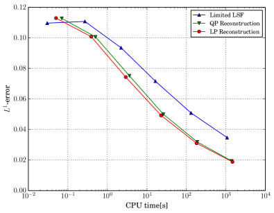
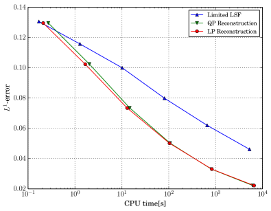
Figure 2: Efficiency of different reconstructions on two sequences of meshes of varying resolution for the solid body rotation benchmark problem.

4.3 Euler equations of gas dynamics

In this final section we consider the $d$-dimensional Euler equations of gas dynamics,

$$\partial_{t}U+\nabla\cdot F(U)=0,$$

where $U=(\rho,\rho v,E)\in\mathbb{R}^{d+2}$ is the vector of conserved quantities, i.e., the density $\rho$, the momentum $\rho v$, and the total energy density $E$. By $v\in\mathbb{R}^{d}$ we denote the primitive particle velocity. The convective flux is given by

$$F(U)=\begin{pmatrix}\rho v\\ \rho v\otimes v+p\,\mathbb{I}_{d}\\ (E+p)v\end{pmatrix}\in\mathbb{R}^{(d+2)\times d},$$

where $\mathbb{I}_{d}$ denotes the $d$-dimensional identity matrix. The pressure $p=p(U)$ is given by the equation of state $p(U)=(\gamma-1)\left(E-\tfrac{\rho}{2}\lvert v\rvert^{2}\right)$ with the adiabatic constant $\gamma=$1.4$$. A state $U$ is considered physical if the density $\rho$ and the pressure $p$ are strictly positive. The set of states is thus given by

$$\mathcal{U}=\bigl{\{}U\in\mathbb{R}^{d+2}\mid\rho>0\text{ and }p>0\bigr{\}}.$$

It is well-known that unphysical values in an approximate solution typically lead to the immediate break-down of a numerical simulation. Therefore, we use a further stabilized modification of the QP reconstruction, Definition 3.2, to the stabilization of the finite volume scheme (2) applied to the vector of primitive variables $W=(\rho,v,E)$. For all $E\in\mathcal{G}$ we consider a modified set of locally admissible linear functions

$$\mathcal{W}^{\prime}(E;u)=\bigl{\{}W\in[P^{1}(\mathbb{R}^{d})]^{d+2}\mid W(x_{E})=W_{E}\text{ and }\\ \min\{W_{E},W_{E,E^{\prime}}\}\leq W(x_{E,E^{\prime}})\leq\max\{W_{E},W_{E,E^{\prime}}\}\text{ for all }E^{\prime}\in\mathcal{N}(E)\bigr{\}},$$

such that all admissible polynomials are physical at least in the midpoints of inter-element intersections. To this end we define the intermediate values $W_{E,E^{\prime}}$, $E^{\prime}\in\mathcal{N}(E)$, $e=E\cap E^{\prime}$,

$$W_{E,E^{\prime}}=\frac{\lvert x_{E^{\prime}}-x_{e}\rvert}{\lvert x_{E}-x_{e}\rvert+\lvert x_{E^{\prime}}-x_{e}\rvert}\,W_{E}+\frac{\lvert x_{E}-x_{e}\rvert}{\lvert x_{E}-x_{e}\rvert+\lvert x_{E^{\prime}}-x_{e}\rvert}W_{E^{\prime}}.$$

We define the positivity-preserving reconstruction operator $\mathcal{R}^{\prime}:X^{0}_{\mathcal{G}}\rightarrow X^{1}_{\mathcal{G}}$ such that for each element $E\in\mathcal{G}$ the reconstruction is the best positivity-preserving $w_{E}\in\mathcal{W}^{\prime}(E;u)$ that fits the piecewise constant data in a least-squares sense.

We are interested in the solution of the three-dimensional shock tube experiment. The computational domain is a cylinder $\Omega=\bigl{\{}x\in\mathbb{R}^{3}\mid-1<x_{1}<1\text{ and }\sqrt{x_{2}^{2}+x_{3}^{2}}<0.2\bigr{\}}.$ In primitive variables, the initial data is given by

$$W(\cdot,0)=\begin{cases}W_{L}&\text{if $x_{1}<0$},\\ W_{R}&\text{otherwise}.\end{cases}$$

The left and right states $W_{L},W_{R}$ for two different test settings are chosen as in [13, Chapter 4.3], see Table 2. The first test problem is known as Sod test problem; its solution consists of a left rarefaction, a contact discontinuity and a right shock. The second test problem is the so-called 123 problem; in this case the solution consists of two rarefactions and a trivial stationary contact discontinuity. The latter benchmark test is particularly challenging as small densities and pressures occur. We solve the Riemann problems for times $t\leq 0.5$ in case of the Sod problem, and for times $t\leq 0.15$ in case of the p123 problem. At the left and right boundary, we prescribe $W=W_{L}$ and $W=W_{R}$, respectively. Otherwise, slip boundary conditions are imposed. The solutions can be computed in a quasi-exact manner as in case of the one-dimensional Euler equations, see, e.g., [13].

Table 2: Initial left and right states in primitive variables for the three-dimensional shock tube experiments.

	$W_{L}$						$W_{R}$
	$\rho$	$v_{1}$	$v_{2}$	$v_{3}$	$p$		$\rho$	$v_{1}$	$v_{2}$	$v_{3}$	$p$
Sod problem	$1$	$0$	$0$	$0$	$1$		$0.125$	$0$	$0$	$0$	$0.1$
p123 problem	$1$	$-2$	$0$	$0$	$0.4$		$1$	$2$	$0$	$0$	$0.4$

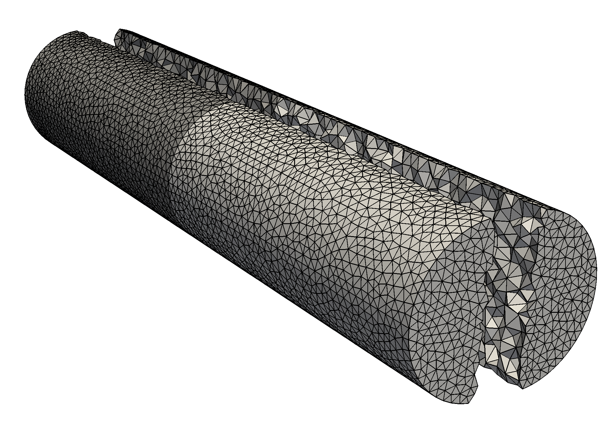
Figure 3: Unstructured tetrahedral mesh for the discretization of the three-dimensional shock tube.

The computational domain is discretized by a series of unstructured, affine tetrahedral grids. Instead of refining the coarsest grid several times, each grid was created separately using the Gmsh mesh generator [8]. It was ensured that the discontinuity in the initial data is exactly resolved by the grid. An example grid is shown in Figure 3. For the MUSCL-type scheme, we use a Harten-Lax-van Leer (HLL) numerical flux. For each grid we computed the $L^{1}$-errors against the quasi-exact solution in primitive variables; the results are shown in Table 3. The experimental order of convergence of roughly $0.85$ for the Sod problem and $0.8$ for the p123-problem is significantly higher than the $0.5$ expected from a first-order scheme.

Table 3: Three-dimensional shock tube experiment, $L^{1}$-errors and convergence rates against the quasi-exact solutions to the Riemann problems under consideration.

				Sod problem			p123 problem
Elements		$h_{\mathcal{G}}$		$\|W-W_{\mathcal{G}}\|_{L^{1}}$	EOC		$\|W-W_{\mathcal{G}}\|_{L^{1}}$	EOC
$288$		$3.48\text{\times}{10}^{-01}$		$4.05\text{\times}{10}^{-02}$	—		$6.21\text{\times}{10}^{-02}$	—
$1680$		$2.13\text{\times}{10}^{-01}$		$2.57\text{\times}{10}^{-02}$	$0.93$		$4.39\text{\times}{10}^{-02}$	$0.71$
$9937$		$1.11\text{\times}{10}^{-01}$		$1.46\text{\times}{10}^{-02}$	$0.86$		$2.54\text{\times}{10}^{-02}$	$0.83$
$71\,788$		$5.66\text{\times}{10}^{-02}$		$8.49\text{\times}{10}^{-03}$	$0.81$		$1.48\text{\times}{10}^{-02}$	$0.81$
$559\,593$		$2.88\text{\times}{10}^{-02}$		$4.73\text{\times}{10}^{-03}$	$0.87$		$8.55\text{\times}{10}^{-03}$	$0.82$
$4\,396\,447$		$1.50\text{\times}{10}^{-02}$		$2.65\text{\times}{10}^{-03}$	$0.89$		$5.28\text{\times}{10}^{-03}$	$0.74$

5 Conclusion

In this paper we proposed a new QP reconstruction method for MUSCL-type finite volume schemes. For each grid element we computed the best admissible fit in a least-squares sense. We showed that the QP reconstruction generalizes the multidimensional Minmod reconstruction for Cartesian meshes. No restrictions to the grid dimension, the conformity of the grid or the shape of individual grid elements were made. The local cell problems only involve data associated with direct neighbors of a grid element and thus preserve the locality of the numerical method. We compared our reconstruction against similar techniques proposed in the literature. By numerical experiments, we showed that the minimization problems are indeed inexpensive to solve and yield a more accurate and efficient approximation.

References

• Alkämper et al. [2016] M. Alkämper, A. Dedner, R. Klöfkorn, and M. Nolte. The DUNE-ALUGrid module. Arch. Numer. Softw., 4(1):1–28, 2016.
• Barth and Jespersen [1989] T. J. Barth and D. C. Jespersen. The design and application of upwind schemes on unstructured meshes. Preprint AIAA-89-0366, American Institute of Aeronautics and Astronautics, 1989.
• Bastian et al. [2008] P. Bastian, M. Blatt, A. Dedner, C. Engwer, R. Klöfkorn, M. Ohlberger, and O. Sander. A generic grid interface for parallel and adaptive scientific computing. part I: Abstract framework. Computing, 82(2–3):103–119, 2008.
• Blatt et al. [2016] M. Blatt, A. Burchardt, A. Dedner, C. Engwer, J. Fahlke, B. Flemish, C. Gersbacher, C. Gräser, F. Gruber, C. Grüninger, D. Kempf, R. Klöfkorn, T. Malkmus, S. Müthing, M. Nolte, M. Piatowski, and O. Sander. The Distributed and Unified Numerics Enviromment, version 2.4. Arch. Numer. Softw., 4(100):13–29, 2016.
• Buffard and Clain [2010] T. Buffard and S. Clain. Monoslope and multislope MUSCL methods for unstructured meshes. J. Comput. Phys., 229(10):3745–3776, May 2010.
• Chen and Li [2016] L. Chen and R. Li. An integrated linear reconstruction for finite volume scheme on unstructured grids. J. Sci. Comput., 68(3):1172–1197, 2016.
• Dedner and Klöfkorn [2011] A. Dedner and R. Klöfkorn. A generic stabilization approach for higher order discontinuous Galerkin methods for convection dominated problems. J. Sci. Comput., 47(3):365–388, 2011.
• Geuzaine and Remacle [2009] C. Geuzaine and J.-F. Remacle. Gmsh: A 3-D finite element mesh generator with built-in pre- and post-processing facilities. Int. J. Numer. Meth. Eng., 79(11):1309–1331, 2009.
• Hubbard [1999] M. E. Hubbard. Multidimensional slope limiters for MUSCL-type finite volume schemes on unstructured grids. J. Comput. Phys., 155(10):54–74, 1999.
• Kröner [1997] D. Kröner. Numerical Schemes for Conservation Laws. Wiley-Teubner, 1997.
• LeVeque [1996] R. J. LeVeque. High-resolution conservative algorithms for advection in incompressible flow. SIAM J. Numer. Anal., 33(2):627–665, 1996.
• May and Berger [2013] S. May and M. Berger. Two-dimensional slope limiters for finite volume schemes on non-coordinate-aligned meshes. SIAM J. Sci. Comput., 35(5):A2163–A2187, 2013.
• Toro [1997] E. F. Toro. Riemann Solvers and Numerical Methods for Fluid Dynamics. Springer-Verlag Berlin Heidelberg, 1997.
• van Leer [1979] B. van Leer. Towards the ultimate conservative difference scheme. V. A second-order sequel to Godunov’s method. J. Comput. Phys., 32(1):101–136, 1979.