Accelerated Orthogonal Least-Squares for Large-Scale Sparse Reconstruction

Abstract

We study the problem of inferring a sparse vector from random linear combinations of its components. We propose the Accelerated Orthogonal Least-Squares (AOLS) algorithm that improves performance of the well-known Orthogonal Least-Squares (OLS) algorithm while requiring significantly lower computational costs. While OLS greedily selects columns of the coefficient matrix that correspond to non-zero components of the sparse vector, AOLS employs a novel computationally efficient procedure that speeds up the search by anticipating future selections via choosing $L$ columns in each step, where $L$ is an adjustable hyper-parameter. We analyze the performance of AOLS and establish lower bounds on the probability of exact recovery for both noiseless and noisy random linear measurements. In the noiseless scenario, it is shown that when the coefficients are samples from a Gaussian distribution, AOLS with high probability recovers a $k$-sparse $m$-dimensional sparse vector using ${\cal O}(k\log\frac{m}{k+L-1})$ measurements. Similar result is established for the bounded-noise scenario where an additional condition on the smallest nonzero element of the unknown vector is required. The asymptotic sampling complexity of AOLS is lower than the asymptotic sampling complexity of the existing sparse reconstruction algorithms. In simulations, AOLS is compared to state-of-the-art sparse recovery techniques and shown to provide better performance in terms of accuracy, running time, or both. Finally, we consider an application of AOLS to clustering high-dimensional data lying on the union of low-dimensional subspaces and demonstrate its superiority over existing methods.

Keywords: sparse recovery, compressed sensing, orthogonal least-squares, orthogonal matching pursuit, subspace clustering

1 Introduction

The task of estimating sparse signal from a few linear combinations of its components is readily cast as the problem of finding a sparse solution to an underdetermined system of linear equations. Sparse recovery is encountered in many practical scenarios, including compressed sensing [1], subspace clustering [2, 3], sparse channel estimation [4, 5], compressive DNA microarrays [6], and a number of other applications in signal processing and machine learning [7, 8, 9]. Consider the linear measurement model

$${{\mathbf{y}}={\mathbf{A}}{\mathbf{x}}+{\boldsymbol{\nu}}},$$ (1)

where ${\mathbf{y}}\in{\mathbb{R}}^{n}$ denotes the vector of observations, ${\mathbf{A}}\in{\mathbb{R}}^{n\times m}$ is the coefficient matrix (i.e., a collection of features) assumed to be full rank (generally, $n<m$), ${\boldsymbol{\nu}}\in{\mathbb{R}}^{n}$ is the additive measurement noise vector, and ${\mathbf{x}}\in{\mathbb{R}}^{m}$ is an unknown vector assumed to have at most $k$ non-zero components (i.e., $k$ is the sparsity level of ${\mathbf{x}}$). Finding a sparse approximation to ${\mathbf{x}}$ leads to a cardinality-constrained least-squares problem

$$\underset{{\mathbf{x}}}{\text{minimize}} \left\lVert{\mathbf{y}}-{\mathbf{A}}{\mathbf{x}}\right\rVert^{2}_{\_}{2} \left\lVert{\mathbf{x}}\right\rVert_{\_}{0}\leq k,$$ subject to (2)

known to be NP-hard; here $\|\cdot\|_{\_}0$ denotes the $\ell_{\_}0$-norm, i.e., the number of non-zero components of its argument. The high cost of finding the exact solution to (2) motivated development of a number of heuristics that can generally be grouped in the following categories:

1) Convex relaxation schemes. These methods perform computationally efficient search for a sparse solution by replacing the non-convex $\ell_{\_}0$-constrained optimization by a sparsity-promoting $\ell_{\_}1$-norm optimization. It was shown in [10] that such a formulation enables exact recovery of a sufficiently sparse signal from noise-free measurements under certain conditions on ${\mathbf{A}}$ and with $\mathcal{O}(k\log\frac{m}{k})$ measurements. However, while the convexity of $\ell_{\_}{1}$-norm enables algorithmically straightforward sparse vector recovery by means of, e.g., iterative shrinkage-thresholding [11] or alternating direction method of multipliers [12], the complexity of such methods is often prohibitive in settings where one deals with high-dimensional signals.

2) Greedy schemes. These heuristics attempt to satisfy the cardinality constraint directly by successively identifying columns of the coefficient matrix which correspond to non-zero components of the unknown vector. Among the greedy methods for sparse vector reconstruction, the orthogonal matching pursuit (OMP) [13] and Orthogonal Least-Squares (OLS) [14, 15] have attracted particular attention in recent years. Intuitively appealing due to its simple geometric interpretation, OMP is characterized by high speed and competitive performance. In each iteration, OMP selects a column of the coefficient matrix ${\mathbf{A}}$ having the highest correlation with the so-called residual vector and adds it to the set of active columns; then the projection of the observation vector ${\mathbf{y}}$ onto the space spanned by the columns in the active set is used to form a residual vector needed for the next iteration of the algorithm. Numerous modifications of OMP with enhanced performance have been proposed in literature. For instance, instead of choosing a single column in each iteration of OMP, StOMP [16] selects and explores all columns having correlation with a residual vector that is greater than a pre-determined threshold. GOMP[17] employs the similar idea, but instead of thresholding, a fixed number of columns is selected per iteration. CoSaMP algorithm [18] identifies columns with largest proximity to the residual vector, uses them to find a least-squares approximation of the unknown signal, and retains only significantly large entries in the resulting approximation. Additionally, necessary and sufficient conditions for exact reconstruction of sparse signals using OMP have been established. Examples of such results include analysis under Restricted Isometry Property (RIP) [19, 20, 21], and recovery conditions based on Mutual Incoherence Property (MIP) and Exact Recovery Condition (ERC) [22, 23, 24]. For the case of random measurements, performance of OMP was analyzed in [25, 26]. Tropp et al. in [25] showed that in the noise-free scenario, ${\cal O}\left(k\log m\right)$ measurements is adequate to recover $k$-sparse $m$-dimensional signals with high probability. In [27], this result was extended to the asymptotic setting of noisy measurements in high signal-to-noise ratio (SNR) under the assumption that the entries of ${\mathbf{A}}$ are i.i.d Gaussian and that the length of the unknown vector approaches infinity. Recently, the asymptotic sampling complexity of OMP and GOMP is improved to ${\cal O}(k\log\frac{m}{k})$ in [28] and [29], respectively.

Recently, performance of OLS was analyzed in the sparse signal recovery settings with deterministic coefficient matrices. In [30], OLS was analyzed in the noise-free scenario under Exact Recovery Condition (ERC), first introduced in[22]. Herzet et al. [31] provided coherence-based conditions for sparse recovery of signals via OLS when the nonzero components of ${\bf x}$ obey certain decay conditions. In [32], sufficient conditions for exact recovery are stated when a subset of true indices is available. In [33] an extension of OLS that employs the idea of [16, 17] and identifies multiple indices in each iteration is proposed and its performance is analyzed under RIP. However, all the existing analysis and performance guarantees for OLS pertain to non-random measurements and cannot directly be applied to random coefficient matrices. For instance, the main results in the notable work [28] relies on the assumption of having dictionaries with $\ell_{\_}2$-norm normalized columns while this obviously does not hold in the scenarios where the coefficient matrix is composed of entries that are drawn from a Gaussian distribution.

3) Branch-and-bound schemes. Recently, greedy search heuristics that rely on OMP and OLS to traverse a search tree along paths that represent promising candidates for the support of ${\mathbf{x}}$ have been proposed. For instance, [34, 35] exploit the selection criterion of OMP to construct the search graph while [36, 37] rely on OLS to efficiently traverses the search tree. Although these methods empirically improve the performance of greedy algorithms, they are characterized by exponential computational complexity in at least one parameter and hence are prohibitive in applications dealing with high-dimensional signals.

1.1 Contributions

Motivated by the need for fast and accurate sparse recovery in large-scale setting, in this paper we propose a novel algorithm that efficiently exploits recursive relation between components of the optimal solution to the original $\ell_{\_}0$-constrained least-squares problem (2). The proposed algorithm, referred to as Accelerated Orthogonal Least-Squares (AOLS), similar to GOMP [17] and MOLS [33] exploits the observation that columns having strong correlation with the current residual are likely to have strong correlation with residuals in subsequent iterations; this justifies selection of multiple columns in each iteration and formulation of an overdetermined system of linear equation having solution that is generally more accurate than the one found by OLS or OMP. However, compared to MOLS, our proposed algorithm is orders of magnitude faster and thus more suitable for high-dimensional data applications.

We theoretically analyze the performance of the proposed AOLS algorithm and, by doing so, establish conditions for the exact recovery of the sparse vector ${\mathbf{x}}$ from measurements ${\mathbf{y}}$ in (1) when the entries of the coefficient matrix ${\mathbf{A}}$ are drawn at random from a Gaussian distribution – the first such result under these assumptions for an OLS-based algorithm. We first present conditions which ensure that, in the noise-free scenario, AOLS with high probability recovers the support of ${\mathbf{x}}$ in $k$ iterations (recall that $k$ denotes the number of non-zero entries of ${\bf x}$). Adopting the framework in [25], we further find a lower bound on the probability of performing exact sparse recovery in $k$ iterations and demonstrate that with ${\cal O}\left(k\log\frac{m}{k+L-1}\right)$ measurements AOLS succeeds with probability arbitrarily close to one. Moreover, we extend our analysis to the case of noisy measurements and show that similar guarantees hold if the nonzero element of ${\mathbf{x}}$ with the smallest magnitude satisfies certain condition. This condition implies that to ensure exact support recovery via AOLS in the presence of additive $\ell_{\_}2$-bounded noise, ${\mathrm{SNR}}$ should scale linearly with sparsity level $k$. Our procedure for determining requirements that need to hold for AOLS to perform exact reconstruction follows the analysis of OMP in [25, 27, 26], although with two major differences. First, the variant of OMP analyzed in [25, 27, 26] implicitly assumes that the columns of ${\mathbf{A}}$ are $\ell_{\_}2$-normalized which clearly does not hold if the entries of ${\mathbf{A}}$ are drawn from a Gaussian distribution. Second, the analysis in [25] is for noiseless measurements while [27, 26] essentially assume that ${\mathrm{SNR}}$ is infinite as $k\rightarrow\infty$. To the contrary, our analysis makes neither of those two restrictive assumptions. Moreover, we show that if $m$ is sufficiently greater than $k$, the proposed AOLS algorithm requires ${\cal O}\left(k\log\frac{m}{k+L-1}\right)$ random measurements to perform exact recovery in both noiseless and bounded noise scenarios; this is fewer than ${\cal O}\left(k\log(m-k)\right)$ that was found in [27, 26] to be the asymptotic sampling complexity for OMP, and ${\cal O}\left(k\log\frac{m}{k}\right)$ that was found for MOLS, GOMP, and BP in [33, 29, 38]. Additionally, our analysis framework is recognizably different from that of [28] for OLS. First, in [28] it is assumed that ${\mathbf{A}}$ has $\ell_{\_}2$-normalized columns, and hence the analysis in [28] does not apply to the case of Gaussian matrices, the scenario addressed in this paper for our proposed algorithm. Further, the main result of [28] (see Theorem 3 in [28]) states that OLS exactly recovers a $k$-sparse vector in at most $6k$ iterations if ${\cal O}\left(k\log\frac{m}{k}\right)$ measurements are available. Hence, the OLS results of [28] are not as strong as the AOLS results we establish in the current paper. Our extensive empirical studies verify the theoretical findings and demonstrate that AOLS is more accurate and faster than the competing state-of-the-art schemes.

To further demonstrate efficacy of the proposed techniques, we consider the sparse subspace clustering (SSC) problem that is often encountered in machine learning and computer vision applications. The goal of SSC is to partition data points drawn from a union of low-dimensional subspaces. We propose a SSC scheme that relies on our AOLS algorithm and empirically show significant improvements in accuracy compared to state-of-the-art methods in [3, 39, 2, 40].

1.2 Organization

The remainder of the paper is organized as follows. In Section 2, we specify the notation and overview the classic OLS algorithm. In Section 3, we describe the proposed AOLS algorithm. Section 4 presents analysis of the performance of AOLS for sparse recovery from random measurements. Section 5 presents experiments that empirically verify our theoretical results on sampling requirements of AOLS and benchmark its performance. Finally, concluding remarks are provided in Section 6. Matlab implementation of AOLS is freely available for download from https://github.com/realabolfazl/AOLS/.

2 Preliminaries

2.1 Notation

We briefly summarize notation used in the paper. Bold capital letters refer to matrices and bold lowercase letters represent vectors. Matrix ${\mathbf{A}}\in{\mathbb{R}}^{n\times m}$ is assumed to have full rank; ${\mathbf{A}}_{\_}{ij}$ denotes the $(i,j)$ entry of ${\mathbf{A}}$, ${\mathbf{a}}_{\_}j$ is the $j\textsuperscript{th}$ column of ${\mathbf{A}}$, and ${\mathbf{A}}_{\_}k\in{\mathbb{R}}^{n\times k}$ is one of the ${m}\choose{k}$ submatrices of ${\mathbf{A}}$ (here we assume $k<n<m$). ${\cal L}_{\_}k$ denotes the subspace spanned by the columns of ${\mathbf{A}}_{\_}k$. ${\mathbf{P}}_{\_}k^{\bot}={\mathbf{I}}-{\mathbf{A}}_{\_}k{\mathbf{A}}_{\_}k^{\dagger}$ is the projection operator onto the orthogonal complement of ${\cal L}_{\_}k$ where ${\mathbf{A}}_{\_}K^{\dagger}=\left({\mathbf{A}}_{\_}k^{\top}{\mathbf{A}}_{\_}k\right)^{-1}{\mathbf{A}}_{\_}k^{\top}$ denotes the Moore-Penrose pseudo-inverse of ${\mathbf{A}}_{\_}k$ and ${\mathbf{I}}\in{\mathbb{R}}^{n\times n}$ is the identity matrix. ${\cal I}=\{1,\dots,m\}$ is the set of column indices, ${\cal S}_{\_}{true}$ is the set of indices of nonzero elements of ${\mathbf{x}}$, and ${\cal S}_{\_}i$ is the set of selected indices at the end of the $i\textsuperscript{th}$ iteration of OLS. For a non-scalar object such as matrix ${\mathbf{A}}$, ${\mathbf{A}}\sim{\cal N}\left(0,\frac{1}{n}\right)$ implies that the entries of ${\mathbf{A}}$ are drawn independently from a zero-mean Gaussian distribution with variance $\frac{1}{n}$. Further, for any vector ${\mathbf{c}}\in{\mathbb{R}}^{m}$ define the ordering operator $\mathcal{P}:{\mathbb{R}}^{m}\rightarrow{\mathbb{R}}^{m}$ as $\mathcal{P}({\mathbf{c}})=[{\mathbf{c}}_{\_}{o_{\_}1},\dots,{\mathbf{c}}_{\_}{o_{\_}m}]^{\top}$ such that $|{\mathbf{c}}_{\_}{o_{\_}1}|\leq\dots\leq|{\mathbf{c}}_{\_}{o_{\_}m}|$. Finally, $\mathbf{1}$ denotes the vector of all ones, and $\mathcal{U}(0,q)$ represents the uniform distribution on $[0,q]$.

2.2 The OLS Algorithm

The OLS algorithm sequentially projects columns of ${\mathbf{A}}$ onto a residual vector and selects the one resulting in the smallest residual norm. Specifically, in the $i\textsuperscript{th}$ iteration OLS chooses a new column index $j_{\_}s$ according to

$${j}_{\_}{s}=\arg\!\min_{\_}{j\in{\cal I}\backslash{\cal S}_{\_}{i-1}}{\left\lVert{\mathbf{P}}_{\_}{{\cal S}_{\_}{i-1}\cup\{j\}}^{\bot}{\mathbf{y}}\right\rVert_{\_}2}.$$ (3)

This procedure is computationally more expensive than OMP since in addition to solving a least-squares problem to update the residual vector, orthogonal projections of the columns of ${\mathbf{A}}$ need to be found in each step of OLS. Note that the performances of OLS and OMP are identical when the columns of ${\mathbf{A}}$ are orthogonal. It is worthwhile pointing out the difference between OMP and OLS. In each iteration of OMP, an element most correlated with the current residual is chosen. OLS, on the other hand, selects a column least expressible by previously selected columns which, in turn, minimizes the approximation error.

It can be shown, see, e.g., [41, 30, 42], that the index selection criterion (3) can alternatively be expressed as

$$j_{\_}s=\arg\!\max_{\_}{j\in{\cal I}\backslash{\cal S}_{\_}{i-1}}{\left|{\mathbf{r}}_{\_}{i-1}^{\top}\frac{{\bf P}_{\_}{i-1}^{\bot}{\bf a}_{\_}{j}}{\left\lVert{\bf P}_{\_}{i-1}^{\bot}{\bf a}_{\_}{j}\right\rVert_{\_}2}\right|},$$ (4)

where ${\mathbf{r}}_{\_}{i-1}$ denotes the residual vector in the $i\textsuperscript{th}$ iteration. Moreover, projection matrix needed for the subsequent iteration is related to the current projection matrix according to

$${{\mathbf{P}}}_{\_}{i+1}^{\bot}={{\mathbf{P}}}_{\_}i^{\bot}-\frac{{{\mathbf{P}}}_{\_}i^{\bot}{\mathbf{a}}_{\_}{j_{\_}s}{\mathbf{a}}_{\_}{j_{\_}s}^{\top}{{\mathbf{P}}}_{\_}i^{\bot}}{\left\lVert{{\mathbf{P}}}_{\_}i^{\bot}{\mathbf{a}}_{\_}{j_{\_}s}\right\rVert_{\_}2^{2}}.$$ (5)

It should be noted that ${\mathbf{r}}_{\_}{i-1}$ in (4) can be replaced by ${\mathbf{y}}$ because of the idempotent property of the projection matrix,

$${{\mathbf{P}}}_{\_}i^{\bot}={{{\mathbf{P}}}_{\_}i^{\bot}}^{\top}={{\mathbf{P}}_{\_}i^{\bot}}^{2}.$$ (6)

This substitution reduces complexity of OLS although, when sparsity level $k$ is unknown, the norm of ${\mathbf{r}}_{\_}{i}$ still needs to be computed since it is typically used when evaluating a stopping criterion. OLS is formalized as Algorithm 1.

Input:       ${\mathbf{y}}$, ${\mathbf{A}}$, sparsity level $k$

Output:     recovered support ${\cal S}_{\_}k$, estimated signal $\hat{{\mathbf{x}}}_{\_}{k}$

Initialize:   ${\cal S}_{\_}0=\emptyset$ , ${\bf P}_{\_}0^{\bot}={\bf I}$

  for     $i=1$ to $k$      do

     1. $j_{\_}s=\arg\!\max_{\_}{j\in{\cal I}\backslash{\cal S}_{\_}{i-1}}{\left|{\mathbf{y}}^{\top}\frac{{\bf P}_{\_}{i-1}^{\bot}{\bf a}_{\_}{j}}{\left\lVert{\bf P}_{\_}{i-1}^{\bot}{\bf a}_{\_}{j}\right\rVert_{\_}2}\right|}$ 2. ${\cal S}_{\_}{i}={\cal S}_{\_}{i-1}\cup\{j_{\_}{s}\}$ 3. ${{\mathbf{P}}}_{\_}{i+1}^{\bot}={{\mathbf{P}}}_{\_}i^{\bot}-\frac{{{\mathbf{P}}}_{\_}i^{\bot}{\mathbf{a}}_{\_}{j_{\_}s}{\mathbf{a}}_{\_}{j_{\_}s}^{\top}{{\mathbf{P}}}_{\_}i^{\bot}}{\left\lVert{{\mathbf{P}}}_{\_}i^{\bot}{\mathbf{a}}_{\_}{j_{\_}s}\right\rVert_{\_}2^{2}}$

  end for

  4. $\hat{{\mathbf{x}}}_{\_}{k}={\mathbf{A}}_{\_}{{\cal S}_{\_}{k}}^{\dagger}{\mathbf{y}}$

Algorithm 1 Orthogonal Least-Squares (OLS)

3 A Novel Accelerated Scheme for Sparse Recovery

In this section we describe the AOLS algorithm in detail. The complexity of the OLS and its existing variants such as MOLS [33] is dominated by the so-called identification and update steps, formalized as steps 1 and 3 of Algorithm 1 in Section 2, respectively; in these steps, the algorithm evaluates projections ${\bf P}_{\_}{i-1}^{\bot}{\bf a}_{\_}{j}$ of not-yet-selected columns onto the space spanned by the selected ones and then computes the projection matrix ${\bf P}_{\_}{i}$ needed for the next iteration. This becomes practically infeasible in applications that involve dealing with high-dimensional data, including sparse subspace clustering. To this end, in Theorem 1 below, we establish a set of recursions which significantly reduce the complexity of the identification and update steps without sacrificing the performance. AOLS then relies on these efficient recursions to identify the indices corresponding to nonzero entries of ${\mathbf{x}}$ with a significantly lower computational costs with respect to OLS and MOLS. This is further verified in our simulation studies.

Theorem 1.

Let ${\mathbf{r}}_{\_}{i}$ denote the residual vector in the $i^{th}$ iteration of OLS with ${\mathbf{r}}_{\_}0={\mathbf{y}}$. The identification step (i.e., step 1 in Algorithm 1) in the $(i+1)\textsuperscript{st}$ iteration of OLS can be rephrased as

$$j_{\_}{s}=\arg\!\max_{\_}{j\in{\cal I}\backslash{\cal S}_{\_}i}\left\lVert{\bf q}_{\_}j\right\rVert_{\_}2,$$ (7)

where

$${\bf q}_{\_}j=\frac{{\mathbf{a}}_{\_}j^{\top}{\mathbf{r}}_{\_}{i}}{{\mathbf{a}}_{\_}j^{\top}{\bf t}_{\_}j^{(i)}}{\bf t}_{\_}j^{(i)},\hskip 14.22636pt{\bf t}_{\_}j^{(i+1)}={\bf t}_{\_}j^{(i)}-\frac{{{\bf t}_{\_}j^{(i)}}^{\top}{\mathbf{u}}_{\_}i}{\left\lVert{\mathbf{u}}_{\_}i\right\rVert_{\_}2^{2}}{\mathbf{u}}_{\_}i,$$ (8)

where ${\bf t}_{\_}j^{(0)}={\mathbf{a}}_{\_}j$ for all $j\in\mathcal{I}$. Furthermore, the residual vector ${\mathbf{r}}_{\_}{i+1}$ required for the next iteration is formed as

$${\mathbf{u}}_{\_}{i+1}={\bf q}_{\_}{j_{\_}s},\hskip 14.22636pt{\mathbf{r}}_{\_}{i+1}={\mathbf{r}}_{\_}{i}-{\mathbf{u}}_{\_}{i+1}.$$ (9)

Proof.

Assume that column ${\mathbf{a}}_{\_}{j_{\_}s}$ is selected in the $(i+1)\textsuperscript{st}$ iteration of the algorithm. Define $\bar{{\mathbf{q}}}_{\_}{j}=\frac{{{\mathbf{P}}}_{\_}i^{\bot}{\mathbf{a}}_{\_}{j}}{\left\lVert{{\mathbf{P}}}_{\_}i^{\bot}{\mathbf{a}}_{\_}{j}\right\rVert_{\_}2^{2}}{\mathbf{a}}_{\_}{j}^{\top}{\mathbf{r}}_{\_}i$, $\forall j\in{\cal I}\backslash{\cal S}_{\_}i$. Therefore,

$$\arg\!\max_{\_}{j\in{\cal I}\backslash{\cal S}_{\_}i}{\|\bar{{\mathbf{q}}}_{\_}{j}\|_{\_}2}=\arg\!\max_{\_}{j\in{\cal I}\backslash{\cal S}_{\_}i}{\frac{|{\mathbf{a}}_{\_}{j}^{\top}{\mathbf{r}}_{\_}i|}{\left\lVert{{\mathbf{P}}}_{\_}i^{\bot}{\mathbf{a}}_{\_}{j}\right\rVert_{\_}2}}.$$ (10)

The idempotent property of ${\mathbf{P}}_{\_}i^{\bot}$ implies that the right hand side of (10) is equivalent to the selection rule of OLS in (4). Therefore, $j_{\_}s=\arg\!\max_{\_}{j\in{\cal I}\backslash{\cal S}_{\_}i}{\|\bar{{\mathbf{q}}}_{\_}{j_{\_}s}\|_{\_}2}$. Let us post-multiply both sides of (5) with the observation vector ${\mathbf{y}}$, leading to

$${{\mathbf{P}}}_{\_}{i+1}^{\bot}{\mathbf{y}}={{\mathbf{P}}}_{\_}i^{\bot}{\mathbf{y}}-\frac{{{\mathbf{P}}}_{\_}i^{\bot}{\mathbf{a}}_{\_}{j_{\_}s}{\mathbf{a}}_{\_}{j_{\_}s}^{\top}{{\mathbf{P}}}_{\_}i^{\bot}}{\left\lVert{{\mathbf{P}}}_{\_}i^{\bot}{\mathbf{a}}_{\_}{j_{\_}s}\right\rVert_{\_}2^{2}}{\mathbf{y}}.$$ (11)

Recall that ${\mathbf{r}}_{\_}i={{\mathbf{P}}}_{\_}i^{\bot}{\mathbf{y}}$ to obtain

$${\mathbf{r}}_{\_}{i+1}={\mathbf{r}}_{\_}i-\frac{{{\mathbf{P}}}_{\_}i^{\bot}{\mathbf{a}}_{\_}{j_{\_}s}}{\left\lVert{{\mathbf{P}}}_{\_}i^{\bot}{\mathbf{a}}_{\_}{j_{\_}s}\right\rVert_{\_}2^{2}}{\mathbf{a}}_{\_}{j_{\_}s}^{\top}{\mathbf{r}}_{\_}i={\mathbf{r}}_{\_}i-\bar{{\mathbf{q}}}_{\_}{j_{\_}s}.$$ (12)

Comparing the above expression with (8), one needs to show ${\mathbf{q}}_{\_}{j_{\_}s}=\bar{{\mathbf{q}}}_{\_}{j_{\_}s}$ to complete the proof; this is equivalent to demonstrating $\frac{{\mathbf{P}}_{\_}i^{\bot}{\mathbf{a}}_{\_}{j_{\_}s}}{\left\lVert{\mathbf{P}}_{\_}i^{\bot}{\mathbf{a}}_{\_}{j_{\_}s}\right\rVert_{\_}2^{2}}=\frac{1}{{\mathbf{a}}_{\_}{j_{\_}s}^{\top}{\bf t}_{\_}j^{(i)}}{\bf t}_{\_}j^{(i)}$. Since ${\mathbf{A}}$ is full rank, the selected columns are linearly independent. Let $\{\widetilde{{\mathbf{a}}}_{\_}l\}_{\_}{l=1}^{i}$ denote the collection of columns selected in the first $i$ iterations and let ${\cal L}_{\_}i=\{\widetilde{{\mathbf{a}}}_{\_}1,\dots,\widetilde{{\mathbf{a}}}_{\_}i\}$ denote the subspace spanned by those columns. Consider the orthogonal projection of the selected column ${\mathbf{a}}_{\_}{j_{\_}s}$ onto ${\cal L}_{\_}i$, ${{\mathbf{P}}}_{\_}i^{\bot}{\mathbf{a}}_{\_}{j_{\_}s}$. Clearly, ${{\mathbf{P}}}_{\_}i^{\bot}{\mathbf{a}}_{\_}{j_{\_}s}={\mathbf{a}}_{\_}{j_{\_}s}-{{\mathbf{P}}}_{\_}i{\mathbf{a}}_{\_}{j_{\_}s}$. Noting the idempotent property of ${{\mathbf{P}}}_{\_}i^{\bot}$ and the fact that $\|{\mathbf{a}}_{\_}{j_{\_}S}\|_{\_}2^{2}=\|{{\mathbf{P}}}_{\_}i^{\bot}{\mathbf{a}}_{\_}{j_{\_}s}\|_{\_}2^{2}+\|{{\mathbf{P}}}_{\_}i{\mathbf{a}}_{\_}{j_{\_}s}\|_{\_}2^{2}$, we obtain

$$\frac{{\mathbf{P}}_{\_}i^{\bot}{\mathbf{a}}_{\_}{j_{\_}s}}{\left\lVert{\mathbf{P}}_{\_}i^{\bot}{\mathbf{a}}_{\_}{j_{\_}s}\right\rVert_{\_}2^{2}}=\frac{{\mathbf{a}}_{\_}{j_{\_}s}-{{\mathbf{P}}}_{\_}i{\mathbf{a}}_{\_}{j_{\_}s}}{{\mathbf{a}}_{\_}{j_{\_}s}^{\top}\left({\mathbf{a}}_{\_}{j_{\_}s}-{{\mathbf{P}}}_{\_}i{\mathbf{a}}_{\_}{j_{\_}s}\right)}.$$ (13)

We need to demonstrate that ${{\mathbf{P}}}_{\_}i{\mathbf{a}}_{\_}{j_{\_}s}=\sum_{\_}{l=1}^{i}\frac{{\mathbf{a}}_{\_}{j_{\_}s}^{\top}{\mathbf{u}}_{\_}l}{\left\lVert{\mathbf{u}}_{\_}l\right\rVert_{\_}2^{2}}{\mathbf{u}}_{\_}l$, i.e., $\{{\mathbf{u}}_{\_}l\}_{\_}{l=1}^{i}$ is an orthogonal basis for ${\cal L}_{\_}i$. To this end, we employ an inductive argument. Consider ${\mathbf{u}}_{\_}1$ and ${\mathbf{u}}_{\_}2$ associated with the $1\textsuperscript{st}$ and $2\textsuperscript{nd}$ iterations. Applying (8) yields

$${\mathbf{u}}_{\_}1=\frac{\widetilde{{\mathbf{a}}}_{\_}1^{\top}{\mathbf{r}}_{\_}0}{\|\widetilde{{\mathbf{a}}}_{\_}i\|_{\_}2^{2}}\widetilde{{\mathbf{a}}}_{\_}1,$$ (14)

$${\mathbf{u}}_{\_}2=\frac{\widetilde{{\mathbf{a}}}_{\_}2^{\top}({\mathbf{r}}_{\_}0-{\mathbf{u}}_{\_}1)}{\widetilde{{\mathbf{a}}}_{\_}2^{\top}\left(\widetilde{{\mathbf{a}}}_{\_}2-\frac{\widetilde{{\mathbf{a}}}_{\_}2^{\top}{\mathbf{u}}_{\_}1}{\|{\mathbf{u}}_{\_}1\|_{\_}2^{2}}{\mathbf{u}}_{\_}1\right)}\left(\widetilde{{\mathbf{a}}}_{\_}2-\frac{\widetilde{{\mathbf{a}}}_{\_}2^{\top}{\mathbf{u}}_{\_}1}{\|{\mathbf{u}}_{\_}1\|_{\_}2^{2}}{\mathbf{u}}_{\_}1\right).$$ (15)

It is straightforward to see that $\widetilde{{\mathbf{a}}}_{\_}1^{\top}\left(\widetilde{{\mathbf{a}}}_{\_}2-\frac{\widetilde{{\mathbf{a}}}_{\_}2^{\top}{\mathbf{u}}_{\_}1}{\|{\mathbf{u}}_{\_}1\|_{\_}2^{2}}{\mathbf{u}}_{\_}1\right)=0$; therefore, ${\mathbf{u}}_{\_}1^{\top}{\mathbf{u}}_{\_}2=0$. Now, a collection of orthogonal columns $\{{\mathbf{u}}_{\_}l\}_{\_}{l=1}^{i-1}$ forms a basis for ${\cal L}_{\_}{i-1}$. It follows from (8) that

$${\mathbf{u}}_{\_}i=\frac{\widetilde{{\mathbf{a}}}_{\_}i^{\top}({\mathbf{r}}_{\_}{i-2}-{\mathbf{u}}_{\_}{i-1})}{\widetilde{{\mathbf{a}}}_{\_}i^{\top}\left(\widetilde{{\mathbf{a}}}_{\_}i-\sum_{\_}{l=1}^{i-1}\frac{\widetilde{{\mathbf{a}}}_{\_}i^{\top}{\mathbf{u}}_{\_}l}{\|{\mathbf{u}}_{\_}1\|_{\_}2^{2}}{\mathbf{u}}_{\_}l\right)}\left(\widetilde{{\mathbf{a}}}_{\_}i-\sum_{\_}{l=1}^{i-1}\frac{\widetilde{{\mathbf{a}}}_{\_}i^{\top}{\mathbf{u}}_{\_}l}{\|{\mathbf{u}}_{\_}1\|_{\_}2^{2}}{\mathbf{u}}_{\_}l\right).$$ (16)

Consider ${\mathbf{u}}_{\_}l^{\top}{\mathbf{u}}_{\_}i$ for any $l\in\{1,\dots,i-1\}$. Since the collection $\{{\mathbf{u}}_{\_}l\}_{\_}{l=1}^{i-1}$ is orthogonal, ${\mathbf{u}}_{\_}l^{\top}{\mathbf{u}}_{\_}i$ is proportional to $\widetilde{{\mathbf{a}}}_{\_}l^{\top}\left(\widetilde{{\mathbf{a}}}_{\_}i-\frac{\widetilde{{\mathbf{a}}}_{\_}i^{\top}{\mathbf{u}}_{\_}l}{\|{\mathbf{u}}_{\_}1\|_{\_}2^{2}}{\mathbf{u}}_{\_}l\right)$, which is readily shown to be zero. Consequently, $\{{\mathbf{u}}_{\_}l\}_{\_}{l=1}^{i}$ is an orthogonal basis for ${\cal L}_{\_}i$ and the orthogonal projection of ${\mathbf{a}}_{\_}{j_{\_}s}$ is formed as the Euclidean projection of ${\mathbf{a}}_{\_}{j_{\_}s}$ onto each of the orthogonal vectors ${\mathbf{u}}_{\_}l$. Therefore, ${{\mathbf{P}}}_{\_}i{\mathbf{a}}_{\_}{j_{\_}s}=\sum_{\_}{l=1}^{i}\frac{{\mathbf{a}}_{\_}{j_{\_}s}^{\top}{\mathbf{u}}_{\_}l}{\left\lVert{\mathbf{u}}_{\_}l\right\rVert_{\_}2^{2}}{\mathbf{u}}_{\_}l$. Using a similar inductive argument one can show ${\bf t}_{\_}j^{(i+1)}={\bf t}_{\_}j^{(i)}-\frac{{{\bf t}_{\_}j^{(i)}}^{\top}{\mathbf{u}}_{\_}i}{\left\lVert{\mathbf{u}}_{\_}i\right\rVert_{\_}2^{2}}{\mathbf{u}}_{\_}i$ , which completes the proof. ∎

The geometric interpretation of the recursive equations established in Theorem 1 is stated in Corollary 1.1. Intuitively, after orthogonalizing selected columns, a new column is identified and added it to the subset thus expanding the corresponding subspace.

Corollary 1.1.

Let $\{\widetilde{{\mathbf{a}}}_{\_}l\}_{\_}{l=1}^{i}$ denote the set of columns selected in the first $i$ iterations of the OLS algorithm and let ${\cal L}=\{\widetilde{{\mathbf{a}}}_{\_}1,\dots,\widetilde{{\mathbf{a}}}_{\_}i\}$ be the subspace spanned by these columns. Then $\{{\mathbf{u}}_{\_}l\}_{\_}{l=1}^{i}$ generated according to Theorem 1 forms an orthogonal basis for ${\cal L}_{\_}i$.

Selecting multiple indices per iteration was first proposed in [16, 17] and shown to improve performance while reducing the number of OMP iterations. However, since selecting multiple indices increases computational cost of each iteration, relying on OMP/OLS identification criterion (as in, e.g., [33]) does not necessarily reduce the complexity and may in fact be prohibitive in practice, as we will demonstrate in our simulation results. Motivated by this observation, we rely on recursions derived in Theorem 1 to develop a novel, computationally efficient variant of OLS that we refer to as Accelerated OLS (AOLS) and formalize it as Algorithm 2. The proposed AOLS algorithm starts with $\mathcal{S}_{\_}0=\varnothing$ and, in each step, selects $1\leq L\leq\lfloor\frac{n}{k}\rfloor$ columns of matrix ${\mathbf{A}}$ such that their normalized projections onto the orthogonal complement of the subspace spanned by the previously chosen columns have higher correlation with the residual vector than remaining non-selected columns. That is, in the $i\textsuperscript{th}$ iteration, AOLS identifies $L$ indices $\{{s_{\_}1},\dots,{s_{\_}L}\}\subset\mathcal{I}\backslash\mathcal{S}_{\_}{i-1}$ corresponding to the $L$ largest terms $\|{\mathbf{q}}_{\_}j\|_{\_}2^{2}$. After such indices are identified, AOLS employs (9) to repeatedly update the residual vector required for consecutive iterations. The procedure continues until a stopping criterion (e.g., a predetermined threshold on the norm of the residual vector) is met, or a preset maximum number of iterations is reached.

Remark: As we will show in our simulation results, performance of AOLS is equivalent to that of the MOLS algorithm. However, AOLS is much faster and more suitable for real-world applications involving high-dimensional signals. In fact, it is straightforward to see that the worst case computational costs of Algorithm 1 (and also MOLS) and Algorithm 2 are ${\cal O}\left(mn^{2}k\right)$ and ${\cal O}\left(mnk\right)$, respectively; therefore, AOLS is significantly less complex than the conventional OLS and MOLS algorithms.

Input:       ${\mathbf{y}}$, ${\mathbf{A}}$, sparsity level $k$, threshold $\epsilon$, $1\leq L\leq\lfloor\frac{n}{k}\rfloor$

Output:     recovered support ${\cal S}_{\_}k$, estimated signal $\hat{{\mathbf{x}}}_{\_}{k}$

Initialize:   $i=0$, ${\cal S}_{\_}i=\emptyset$, ${\mathbf{r}}_{\_}i=0$, ${\bf t}_{\_}j^{(i)}={\mathbf{a}}_{\_}j$, ${\mathbf{q}}_{\_}j=\frac{{\mathbf{a}}_{\_}j^{\top}{\mathbf{r}}_{\_}i}{{\mathbf{a}}_{\_}j^{\top}{\bf t}_{\_}j^{(i)}}{\bf t}_{\_}j^{(i)}$ for all $j\in\mathcal{I}$.

  while  $\|{\mathbf{r}}_{\_}i\|_{\_}2\geq\epsilon$ and $i<k$  

     1. Select $\{j_{\_}{s_{\_}1},\dots,j_{\_}{s_{\_}L}\}$ corresponding to $L$ largest terms $\left\lVert{\bf q}_{\_}j\right\rVert_{\_}2$ 2. $i\leftarrow i+1$ 3. ${\cal S}_{\_}{i}={\cal S}_{\_}{i-1}\cup\{j_{\_}{s_{\_}1},\dots,j_{\_}{s_{\_}L}\}$ 4. Perform (9) $L$ times to update $\{{\mathbf{u}}_{\_}{\ell_{\_}1},\dots,{\mathbf{u}}_{\_}{\ell_{\_}L}\}_{\_}{\ell=1}^{i}$ and ${\mathbf{r}}_{\_}i$ 5. ${\mathbf{t}}_{\_}j^{(i)}={\mathbf{t}}_{\_}j^{(i-1)}-\sum_{\_}{l=1}^{L}\frac{{{\mathbf{t}}_{\_}j^{(i-1)}}^{\top}{\mathbf{u}}_{\_}{i_{\_}l}}{\|{\mathbf{u}}_{\_}{i_{\_}l}\|_{\_}2^{2}}{\mathbf{u}}_{\_}{i_{\_}l}$ for all $j\in\mathcal{I}\backslash\mathcal{S}_{\_}i$

  end while

  4. $\hat{{\mathbf{x}}}={\mathbf{A}}_{\_}{{\cal S}_{\_}{i}}^{\dagger}{\mathbf{y}}$

Algorithm 2 Accelerated Orthogonal Least-Squares (AOLS)

4 Performance Analysis of AOLS for sparse recovery

In this section, we first study performance of AOLS in the random measurements and noise-free scenario; specifically, we consider the linear model (1) where the elements of ${\mathbf{A}}$ are drawn from ${\cal N}\left(0,\frac{1}{n}\right)$ and ${\boldsymbol{\nu}}=\mathbf{0}$, and derive conditions for the exact recovery via AOLS. Then we generalize this result to the noisy scenario. First, we begin by stating three lemmas later used in the proofs of main theorems.

4.1 Lemmas

As stated in Section 1, existing analysis of OMP under Gaussian measurements [25, 26] alter the selection criterion to analyze probability of successfull recovery. On the other hand, current analysis of OLS in [28] relies on the assumption that the coefficient matrix has normalized columns and cannot be directly applied to the case of Gaussian measurement, the scenario considered in this paper for analysis of the proposed AOLS algorithm. As part of our contribution, we provide Lemma 2 that states the projection of a random vector drawn from a zero-mean Gaussian distribution onto a random subspace preserves its expected Euclidean norm (within a normalizing factor which is a function of the problem parameters) and is with high probability concentrated around its expected value.

Lemma 2.

Assume that an $n\times m$ coefficient matrix ${\mathbf{A}}$ consists of entries that are drawn independently from ${\cal N}(0,1/n)$ and let ${\mathbf{A}}_{\_}k\in{\mathbb{R}}^{n\times k}$ be a submatrix of ${\mathbf{A}}$. Then, $\forall{\bf u}\in{\mathbb{R}}^{n}$ statistically independent of ${\mathbf{A}}_{\_}k$ drawn according to ${\mathbf{u}}\sim{\cal N}(0,1/n)$, it holds that $\operatorname{\mathbb{E}}\left\lVert{\mathbf{P}}_{\_}k{\mathbf{u}}\right\rVert_{\_}2^{2}=\frac{k}{n}\operatorname{\mathbb{E}}\left\lVert{\mathbf{u}}\right\rVert_{\_}2^{2}$. Moreover, let $c_{\_}0(\epsilon)=\frac{\epsilon^{2}}{4}-\frac{\epsilon^{3}}{6}$. Then,

$$\Pr\{(1-\epsilon)\frac{k}{n}<\left\lVert{\mathbf{P}}_{\_}k{\mathbf{u}}\right\rVert_{\_}2^{2}<(1+\epsilon)\frac{k}{n}\}\geq 1-2e^{-kc_{\_}0(\epsilon)}.$$ (17)

Proof.

See Appendix A. ∎

Lemma 3 (Corollary 2.4.5 in [43]) states inequalities between the maximum and minimum singular values of a matrix and its submatrices.

Lemma 3.

Let ${\mathbf{A}}$, ${\mathbf{B}}$, and ${\mathbf{C}}$ be full rank tall matrices such that ${\mathbf{C}}=[{\mathbf{A}},{\mathbf{B}}]$. Then

$$\sigma_{\_}{\min}\left({\mathbf{A}}\right)\geq\sigma_{\_}{\min}\left({\mathbf{C}}\right), \sigma_{\_}{\max}\left({\mathbf{A}}\right)\leq\sigma_{\_}{\max}\left({\mathbf{C}}\right),$$ (18a)

$$\sigma_{\_}{\min}\left({\mathbf{B}}\right)\geq\sigma_{\_}{\min}\left({\mathbf{C}}\right), \sigma_{\_}{\max}\left({\mathbf{B}}\right)\leq\sigma_{\_}{\max}\left({\mathbf{C}}\right).$$ (18b)

Lemma 4 (Lemma 5.1 in [44]) estabishes bounds on the singular values of ${\mathbf{A}}_{\_}k$, i.e., a submatrix of ${\mathbf{A}}$ with $k$ columns.

Lemma 4.

Let ${\mathbf{A}}\in{\mathbb{R}}^{n\times m}$ denote a matrix with entries that are drawn independently from ${\cal N}(0,1/n)$. Then, for any $0<\delta<1$ and for all ${\mathbf{x}}\in\mathrm{Range}({\mathbf{A}}_{\_}k)$, it holds that

$$\Pr\{|\frac{\|{\mathbf{A}}_{\_}k{\mathbf{x}}\|_{\_}2}{\|{\mathbf{x}}\|_{\_}2}-1|\leq\delta\}\geq 1-2(\frac{12}{\delta})^{k}e^{-nc_{\_}0(\frac{\delta}{2})}.$$ (19)

4.2 Noiseless measurements

In this section we analyze the performance of AOLS when ${\boldsymbol{\nu}}=\mathbf{0}$. The following theorem establishes that when the coefficient matrix consists of entries drawn from ${\cal N}(0,1/n)$ and the measurements are noise-free, AOLS with high probability recovers an unknown sparse vector from the linear combinations of its entries in at most $k$ iterations.

Theorem 5.

Suppose ${\mathbf{x}}\in{\mathbb{R}}^{m}$ is an arbitrary sparse vector with $k<m$ non-zero entries. Let ${\mathbf{A}}\in{\mathbb{R}}^{n\times m}$ be a random matrix with entries drawn independently from ${\cal N}(0,1/n)$. Let $\Sigma$ denote an event wherein given noiseless measurements ${\mathbf{y}}={\mathbf{A}}{\mathbf{x}}$, AOLS can recover ${\mathbf{x}}$ in at most $k$ iterations. Then $\Pr\{\Sigma\}\geq p_{\_}1p_{\_}2p_{\_}3$, where

$$p_{\_}1 =\left(1-2e^{-(n-k+1)c_{\_}0(\epsilon)}\right)^{2},$$ (20)

$$p_{\_}2 =1-2(\frac{12}{\delta})^{k}e^{-nc_{\_}0(\frac{\delta}{2})},\mbox{ and }$$

$$p_{\_}3 =\left(1-\sum_{\_}{i=0}^{k-1}e^{-\frac{n}{k-i}\frac{1-\epsilon}{1+\epsilon}(1-\delta)^{2}}\right)^{m-k-L+1},$$

for any $0<\epsilon<1$ and $0<\delta<1$.

Proof.

As stated, the proof is inspired by the inductive framework first introduced in [25]. We can assume, without a loss of generality, that the nonzero components of ${\mathbf{x}}$ are in the first $k$ locations. This implies that ${\mathbf{A}}$ can be written as ${\mathbf{A}}=\left[\bar{{\mathbf{A}}}\;\;\widetilde{{\mathbf{A}}}\right]$, where $\bar{{\mathbf{A}}}\in{\mathbb{R}}^{n\times k}$ has columns with indices in ${\cal S}_{\_}{true}$ and $\widetilde{{\mathbf{A}}}\in{\mathbb{R}}^{n\times(m-k)}$ has columns with indices in ${\cal I}\backslash{\cal S}_{\_}{true}$. For ${\cal T}_{\_}1\subset{\cal I}$ and ${\cal T}_{\_}2\subset{\cal I}$ such that ${\cal T}_{\_}1\cap{\cal T}_{\_}2=\emptyset$, define

$${\mathbf{b}}_{\_}{j}^{{\cal T}_{\_}1}=\frac{{\mathbf{a}}_{\_}j}{\left\lVert{\mathbf{P}}_{\_}{{\cal T}_{\_}1}^{\bot}{\mathbf{a}}_{\_}j\right\rVert_{\_}2},\hskip 5.69046ptj\in{\cal T}_{\_}2,$$ (21)

where ${\mathbf{P}}_{\_}{{\cal T}_{\_}1}^{\bot}$ denotes the projection matrix onto the orthogonal complement of the subspace spanned by the columns of ${\mathbf{A}}$ with indices in ${\cal T}_{\_}1$. Using the notation of (21), (4) becomes

$$j_{\_}s=\arg\!\max_{\_}{j\in{\cal I}\backslash{\cal S}_{\_}{i-1}}{\left|{\mathbf{r}}_{\_}{i-1}^{\top}{\mathbf{b}}_{\_}{j}^{{\cal S}_{\_}{i-1}}\right|}.$$ (22)

In addition, let ${\boldsymbol{\Phi}}_{\_}{{\cal S}_{\_}i}=[{\mathbf{b}}_{\_}{j}^{{\cal S}_{\_}i}]\in{\mathbb{R}}^{n\times(k-i)}$, $j\in{\cal S}_{\_}{true}\backslash{\cal S}_{\_}i$, and ${\boldsymbol{\Psi}}_{\_}{{\cal S}_{\_}i}=[{\mathbf{b}}_{\_}{j}^{{\cal S}_{\_}i}]\in{\mathbb{R}}^{n\times(m-k)}$, $j\in{\cal I}\backslash{\cal S}_{\_}{true}$. Assume that in the first $i$ iterations AOLS selects columns from ${\cal S}_{\_}{true}$. Let $|\psi_{\_}{o_{\_}1}^{\top}{\mathbf{r}}_{\_}i|\leq\dots\leq|\psi_{\_}{o_{\_}{m-k}}^{\top}{\mathbf{r}}_{\_}i|$ be an ordering of the set $\{|\psi_{\_}1^{\top}{\mathbf{r}}_{\_}i|,\dots,|\psi_{\_}{m-k}^{\top}{\mathbf{r}}_{\_}i|\}$. According to the selection rule in (22), AOLS identifies at least one true column in the $(i+1)\textsuperscript{st}$ iteration if the maximum correlation between ${\mathbf{r}}_{\_}i$ and columns of ${\boldsymbol{\Phi}}_{\_}{{\cal S}_{\_}i}$ is greater than the $|\mathcal{P}({\boldsymbol{\Psi}}_{\_}{{\cal S}_{\_}i}^{\top}{\mathbf{r}}_{\_}i)_{\_}{m-k-L+1}|$. Therefore,

$$\rho({\mathbf{r}}_{\_}i)=\frac{|\mathcal{P}({\boldsymbol{\Psi}}_{\_}{{\cal S}_{\_}i}^{\top}{\mathbf{r}}_{\_}i)_{\_}{m-k-L+1}|}{\|{\boldsymbol{\Phi}}_{\_}{{\cal S}_{\_}i}^{\top}{\mathbf{r}}_{\_}i\|_{\_}\infty}<1$$ (23)

guarantees that AOLS selects at least one true column in the $(i+1)\textsuperscript{st}$ iteration. Hence, $\rho({\mathbf{r}}_{\_}i)<1$ for $i\in\{0,\dots,k-1\}$ ensures recovery of ${\mathbf{x}}$ in $k$ iterations. In other words, $\max_{\_}{i}{\rho({\mathbf{r}}_{\_}i)}<1$ is sufficient condition for AOLS to successfully recover the support of ${\mathbf{x}}$, i.e., if $\Sigma$ denotes the event that AOLS succeeds, then $\Pr\{\Sigma\}\geq\Pr\{\max_{\_}{i}{\rho({\mathbf{r}}_{\_}i)}<1\}$. We may upper bound $\rho({\mathbf{r}}_{\_}i)$ as

$$\rho({\mathbf{r}}_{\_}i)\leq\frac{|\mathcal{P}(\widetilde{{\mathbf{A}}}^{\top}{\mathbf{r}}_{\_}i)_{\_}{m-k-L+1}|}{\|\bar{{\mathbf{A}}}^{\top}{\mathbf{r}}_{\_}i\|_{\_}\infty}\frac{\max_{\_}{j\in{\cal S}_{\_}{true}}{\|{\mathbf{P}}_{\_}i^{\bot}{\mathbf{a}}_{\_}j\|_{\_}2}}{\min_{\_}{j\not\in{\cal S}_{\_}{true}}{\|{\mathbf{P}}_{\_}i^{\bot}{\mathbf{a}}_{\_}j\|_{\_}2}}.$$ (24)

According to Lemma 2,

$$\rho({\mathbf{r}}_{\_}i) \leq\frac{|\mathcal{P}(\widetilde{{\mathbf{A}}}^{\top}{\mathbf{r}}_{\_}i)_{\_}{m-k-L+1}|}{\|\bar{{\mathbf{A}}}^{\top}{\mathbf{r}}_{\_}i\|_{\_}\infty}\sqrt{\frac{1+\epsilon}{1-\epsilon}}\sqrt{\frac{(n-i)/n}{(n-i)/n}}\frac{\operatorname{\mathbb{E}}\|{\mathbf{a}}_{\_}{j_{\_}{\max}}\|_{\_}2}{\operatorname{\mathbb{E}}\|{\mathbf{a}}_{\_}{j_{\_}{\min}}\|_{\_}2}$$ (25)

$$=\sqrt{\frac{1+\epsilon}{1-\epsilon}}\frac{|\mathcal{P}(\widetilde{{\mathbf{A}}}^{\top}{\mathbf{r}}_{\_}i)_{\_}{m-k-L+1}|}{\|\bar{{\mathbf{A}}}^{\top}{\mathbf{r}}_{\_}i\|_{\_}\infty}$$

with probability exceeding $p_{\_}1=\left(1-2e^{-(n-k+1)c_{\_}0(\epsilon)}\right)^{2}$ for $0\leq i<k$. Let $c_{\_}1(\epsilon)=\sqrt{\frac{1-\epsilon}{1+\epsilon}}$. Using a simple norm inequality and exploiting the fact that $\bar{{\mathbf{A}}}^{\top}{\mathbf{r}}_{\_}i$ has at most $k-i$ nonzero entries leads to

$$\rho({\mathbf{r}}_{\_}i)\leq\frac{\sqrt{k-i}}{c_{\_}1(\epsilon)}\frac{|\mathcal{P}(\widetilde{{\mathbf{A}}}^{\top}{\mathbf{r}}_{\_}i)_{\_}{m-k-L+1}|}{\|\bar{{\mathbf{A}}}^{\top}{\mathbf{r}}_{\_}i\|_{\_}2}=\frac{\sqrt{k-i}}{c_{\_}1(\epsilon)}\|\widetilde{{\mathbf{A}}}^{\top}\widetilde{{\mathbf{r}}}_{\_}i\|_{\_}\infty,$$ (26)

where $\widetilde{{\mathbf{r}}}_{\_}i={\mathbf{r}}_{\_}i/\|\bar{{\mathbf{A}}}^{\top}{\mathbf{r}}_{\_}i\|_{\_}2$. According to Lemma 4, for any $0<\delta<1$, $\Pr\{\|\widetilde{{\mathbf{r}}}_{\_}i\|_{\_}2\leq\frac{1}{1-\delta}\}\geq 1-2(\frac{12}{\delta})^{k}e^{-nc_{\_}0(\frac{\delta}{2})}=p_{\_}2$. Subsequently,

$$\Pr\{\Sigma\} \geq p_{\_}1p_{\_}2\Pr\{\max_{\_}{0\leq i<k}{|\mathcal{P}(\widetilde{{\mathbf{A}}}^{\top}{\mathbf{r}}_{\_}i)_{\_}{m-k-L+1}|}<c_{\_}1(\epsilon)\}$$ (27)

$$\geq p_{\_}1p_{\_}2\prod_{\_}{j=1}^{m-k-L+1}\Pr\{\max_{\_}{0\leq i<k}{\left|\widetilde{{\mathbf{a}}}_{\_}{o_{\_}j}^{\top}\widetilde{{\mathbf{r}}}_{\_}i\sqrt{k-i}\right|}<c_{\_}1(\epsilon)\}$$

$$=p_{\_}1p_{\_}2\Pr\{\max_{\_}{0\leq i<k}{\left|\widetilde{{\mathbf{a}}}_{\_}{o_{\_}1}^{\top}\widetilde{{\mathbf{r}}}_{\_}i\sqrt{k-i}\right|}<c_{\_}1(\epsilon)\}^{m-k-L+1},$$

where we used the assumption that the columns of $\widetilde{{\mathbf{A}}}$ are independent. Note that the random vectors $\{\widetilde{{\mathbf{r}}}_{\_}i\sqrt{k-i}\}_{\_}{i=0}^{k-1}$ are bounded with probability exceeding $p_{\_}2$ and are statistically independent of $\widetilde{{\mathbf{A}}}$. Now, recall that the entries of ${\mathbf{A}}$ are drawn independently from ${\cal N}\left(0,\frac{1}{n}\right)$. Since the random variable $X_{\_}{i}=\widetilde{{\mathbf{a}}}_{\_}{o_{\_}1}^{\top}\widetilde{{\mathbf{r}}}_{\_}i\sqrt{k-i}$ is distributed as ${\cal N}(0,\sigma^{2})$ with $\sigma^{2}\leq\frac{k-i}{n(1-\delta)^{2}}$, by using a Gaussian tail bound and Boole’s inequality it is straightforward to show that

$$\Pr\{\max_{\_}{0\leq i<k}{\left|X_{\_}{i}\right|<c_{\_}1(\epsilon)}\}\geq 1-\sum_{\_}{i=0}^{k-1}e^{-\frac{n}{k-i}c_{\_}1(\epsilon)^{2}(1-\delta)^{2}}.$$ (28)

Thus, $\Pr\{\Sigma\}\geq p_{\_}1p_{\_}2p_{\_}3$, where

$$p_{\_}3=\left(1-\sum_{\_}{i=0}^{k-1}e^{-\frac{n}{k-i}c_{\_}1(\epsilon)^{2}(1-\delta)^{2}}\right)^{m-k-L+1}.$$

This completes the proof. ∎

Using the result of Theorem 5, one can numerically show that AOLS successfully recovers $k$-sparse ${\mathbf{x}}$ if the number of measurements is linear in $k$ (sparsity) and logarithmic in $\frac{m}{k+L-1}$.

Corollary 5.1.

Let ${\mathbf{x}}\in{\mathbb{R}}^{m}$ be an arbitrary $k$-sparse vector and let ${\mathbf{A}}\in{\mathbb{R}}^{n\times m}$ denote a matrix with entries that are drawn independently from ${\cal N}(0,1/n)$; moreover, assume that $n\geq\max\{\frac{6}{C_{\_}1}k\log\frac{m}{(k+L-1)\sqrt[3]{\beta}},\frac{C_{\_}2k+\log\frac{8}{\beta^{2}}}{C_{\_}3}\}$, where $0<\beta<1$ and $C_{\_}1$, $C_{\_}2$, and $C_{\_}3$ are positive constants independent of $\beta$, $n$, $m$, and $k$. Given noiseless measurements ${\mathbf{y}}={\mathbf{A}}{\mathbf{x}}$, AOLS can recover ${\mathbf{x}}$ in at most $k$ iterations with probability of success exceeding $1-\beta^{2}$.

Proof.

Let us first take a closer look at $p_{\_}3$. Note that $(1-x)^{l}\geq 1-lx$ is valid for $x\leq 1$ and $l\geq 1$; since replacing $k-i$ with $k$ in the expression for $p_{\_}3$ in (20) decreases $p_{\_}3$, $k(m-k-L+1)\leq\frac{1}{4}(\frac{m}{k+L-1})^{6}$ for $m>(k+L-1)^{3/2}$ and we obtain

$$p_{\_}3\geq 1-\frac{1}{4}(\frac{m}{k+L-1})^{6}e^{-C_{\_}1\frac{n}{k}},$$ (29)

where $C_{\_}1=\frac{1-\epsilon}{1+\epsilon}(1-\delta)^{2}>0$. Multiplying both sides of (29) with $p_{\_}1$ and $p_{\_}2$ and discarding positive higher order terms leads to

$$\Pr\{\Sigma\}\geq 1-\frac{1}{4}(\frac{m}{k+L-1})^{6}e^{-C_{\_}1\frac{n}{k}}-2e^{\log\frac{12}{\delta}k}e^{-nc_{\_}0(\frac{\delta}{2})}-4e^{c_{\_}0(\epsilon)k}e^{-nc_{\_}0(\epsilon)}.$$ (30)

This inequality is readily simplified by defining positive constants $C_{\_}2=\max_{\_}{0<\epsilon,\delta<1}{\{\log\frac{12}{\delta},c_{\_}0(\epsilon)\}}$ and $C_{\_}3=\min_{\_}{0<\epsilon,\delta<1}{\{c_{\_}0(\frac{\delta}{2}),c_{\_}0(\epsilon)\}}$,

$$\Pr\{\Sigma\}\geq 1-\frac{1}{4}(\frac{m}{k+L-1})^{6}e^{-C_{\_}1\frac{n}{k}}-6e^{C_{\_}2k}e^{-nC_{\_}3}.$$ (31)

We need to show that $\Pr\{\Sigma\}\geq 1-\beta^{2}$. To this end, it suffices to demonstrate that

$$\beta^{2}\geq\frac{1}{4}(\frac{m}{k+L-1})^{6}e^{-C_{\_}1\frac{n}{k}}+6e^{C_{\_}2k}e^{-nC_{\_}3}.$$ (32)

Let $n\geq\frac{C_{\_}2k+\log\frac{8}{\beta^{2}}}{C_{\_}3}$. This ensures $6e^{C_{\_}2k}e^{-nC_{\_}3}\leq\frac{3\beta^{2}}{4}$ and thus gives the desired result. Moreover,

$$n\geq\max\{\frac{6}{C_{\_}1}k\log\frac{m}{(k+L-1)\sqrt[3]{\beta}},\frac{C_{\_}2k+\log\frac{8}{\beta^{2}}}{C_{\_}3}\}$$ (33)

guarantees that $\Pr\{\Sigma\}\geq 1-\beta^{2}$ with $0<\beta<1$. ∎

Remark 1: Note that when $k\to\infty$ (and so do $m$ and $n$), $p_{\_}1$, $p_{\_}2$, and $p_{\_}3$ are very close to $1$. Therefore, one may assume very small $\epsilon$ and $\delta$ which implies $C_{\_}1\approx 1$.

4.3 Noisy measurements

We now turn to the general case of noisy random measurements and study the conditions under which AOLS with high probability exactly recovers support of ${\mathbf{x}}$ in at most $k$ iterations.

Theorem 6.

Let ${\mathbf{x}}\in{\mathbb{R}}^{m}$ be an arbitrary $k$-sparse vector and let ${\mathbf{A}}\in{\mathbb{R}}^{n\times m}$ denote a matrix with entries that are drawn independently from ${\cal N}(0,1/n)$. Given the noisy measurements ${\mathbf{y}}={\mathbf{A}}{\mathbf{x}}+{\boldsymbol{\nu}}$ where $\|{\boldsymbol{\nu}}\|_{\_}2\leq\epsilon_{\_}{\boldsymbol{\nu}}$, and ${\boldsymbol{\nu}}$ is independent of ${\mathbf{A}}$ and ${\mathbf{x}}$, if $\min_{\_}{{\mathbf{x}}_{\_}j\neq 0}{|{\mathbf{x}}_{\_}j|}\geq(1+\delta+t)\epsilon_{\_}{{\boldsymbol{\nu}}}$ for any $t>0$, AOLS can recover ${\mathbf{x}}$ in at most $k$ iterations with probability of success ${\mathbf{P}}\{\Sigma\}\geq p_{\_}1p_{\_}2p_{\_}3$ where

$$p_{\_}1 =\left(1-2e^{-(n-k+1)c_{\_}0(\epsilon)}\right)^{2}$$ (34)

$$p_{\_}2 =1-2(\frac{12}{\delta})^{k}e^{-nc_{\_}0(\frac{\delta}{2})},\mbox{ and }$$

$$p_{\_}3 =\left(1-\sum_{\_}{i=0}^{k-1}e^{-\frac{n\frac{1-\epsilon}{1+\epsilon}(1-\delta)^{4}}{k\left[\frac{1}{(k-i)t^{2}}+(1+\delta)^{2}\right]}}\right)^{m-k-L+1}$$

for any $0<\epsilon<1$, $0<\delta<1$.

Proof.

See Appendix B. ∎

Remark 2: If we define ${\mathrm{SNR}}=\frac{\|{\mathbf{A}}{\mathbf{x}}\|_{\_}2^{2}}{\|{\boldsymbol{\nu}}\|_{\_}2^{2}}$, the condition $\min_{\_}{{\mathbf{x}}_{\_}j\neq 0}{|{\mathbf{x}}_{\_}j|}\geq(1+\delta+t)\epsilon_{\_}{\boldsymbol{\nu}}$ implies

$${\mathrm{SNR}}\approx k(1+\delta+t)^{2},$$ (35)

which suggests that for exact support recovery via OLS, ${\mathrm{SNR}}$ should scale linearly with sparsity level.

Corollary 6.1.

Let ${\mathbf{x}}\in{\mathbb{R}}^{m}$ be an arbitrary $k$-sparse vector and let ${\mathbf{A}}\in{\mathbb{R}}^{n\times m}$ denote a matrix with entries that are drawn independently from ${\cal N}(0,1/n)$; moreover, assume that $n\geq\max\{\frac{6}{C_{\_}1}k\log\frac{m}{(k+L-1)\sqrt[3]{\beta}},\frac{C_{\_}2k+\log\frac{8}{\beta^{2}}}{C_{\_}3}\}$ where $0<\beta<1$ and $C_{\_}1$, $C_{\_}2$, and $C_{\_}3$ are positive constants that are independent of $\beta$, $n$, $m$, and $k$. Given the noisy measurements ${\mathbf{y}}={\mathbf{A}}{\mathbf{x}}+{\boldsymbol{\nu}}$ where ${\boldsymbol{\nu}}\sim{\cal N}(0,\sigma^{2})$ is independent of ${\mathbf{A}}$ and ${\mathbf{x}}$, if $\min_{\_}{{\mathbf{x}}_{\_}j\neq 0}{|{\mathbf{x}}_{\_}j|}\geq C_{\_}4\|{\boldsymbol{\nu}}\|_{\_}2$ for some $C_{\_}4>1$, AOLS can recover ${\mathbf{x}}$ in at most $k$ iterations with probability of success exceeding $1-\beta^{2}$.

Proof.

The proof follows the steps of the proof to Corollary 5.1, leading us to constants $C_{\_}1=\frac{1-\epsilon}{1+\epsilon}(1-\delta)^{4}(1+t^{2}(1+\delta)^{2})^{-1}$, $C_{\_}2=\max_{\_}{0<\epsilon,\delta<1}{\{\log\frac{12}{\delta},c_{\_}0(\epsilon)\}}>0$, $C_{\_}3=\min_{\_}{0<\epsilon,\delta<1}{\{c_{\_}0(\frac{\delta}{2}),c_{\_}0(\epsilon)\}}>0$, and $C_{\_}4=(1+\delta+t)$. ∎

Remark 3: In general, for the case of noisy measurements $C_{\_}1$ is smaller than that of the noiseless setting, implying a more demanding sampling requirement for the former.

5 Simulations

5.1 Confirmation of theoretical results

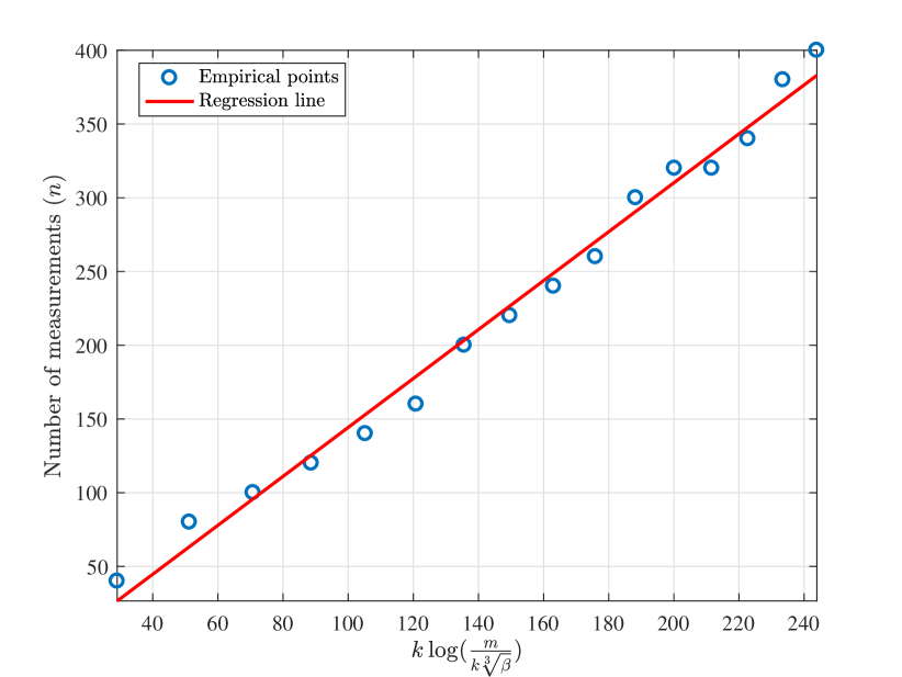
Fig. 1: Number of noiseless measurements required for sparse reconstruction with $\beta^{2}=0.05$ when $m=1024$. The regression line is $n=2.0109$ $k\log(\frac{m}{k\sqrt[3]{\beta}})$ with the coefficient of determination $R^{2}=0.9888$.

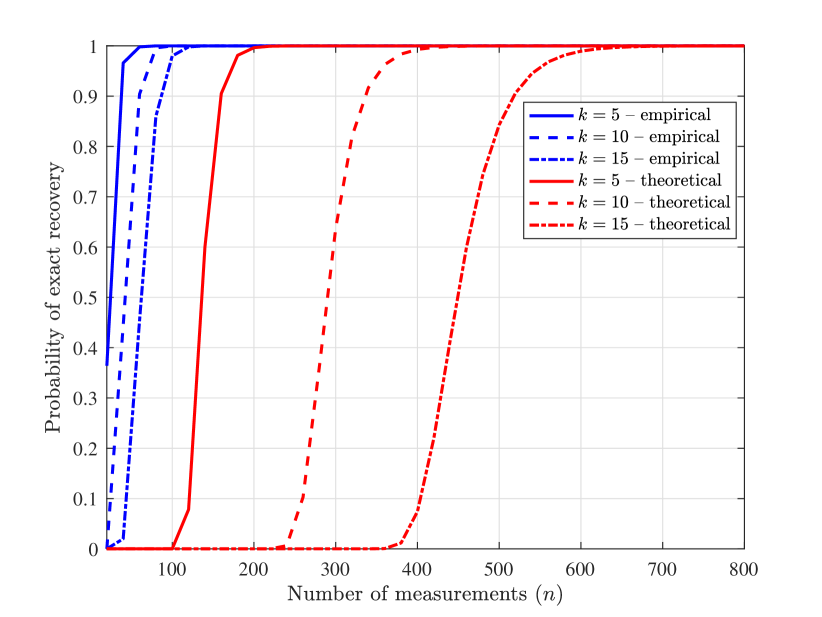
Fig. 2: A comparison of the theoretical probability of exact recovery provided by Theorem 5 with the empirical one, where $m=1024$ and the non-zero elements of ${\mathbf{x}}$ are drawn independently from a normal distribution.

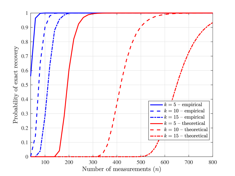
Fig. 3: A comparison of the theoretical probability of exact recovery provided by Theorem 6 with the empirical one, where $m=1024$ and non-zero elements ${\mathbf{x}}$ are set to $(1+\delta+20)\|{\boldsymbol{\nu}}\|_{\_}2$.

In this section, we verify our theoretical results by comparing them to the empirical ones obtained via Monte Carlo simulations.

First, we consider the results of Corollary 5.1 with $L=1$. In each trial, we select locations of the nonzero elements of ${\mathbf{x}}$ uniformly at random and draw those elements from a normal distribution. Entries of the coefficient matrix ${\mathbf{A}}$ are also generated randomly from ${\cal N}(0,\frac{1}{n})$. Fig. 1 plots the number of noiseless measurement $n$ needed to achieve at least $0.95$ probability of perfect recovery (i.e., $\beta^{2}=0.05$) as a function of $k\log(\frac{m}{k\sqrt[3]{\beta}})$. The length of the unknown vector ${\mathbf{x}}$ here is set to $m=1024$, and the results (shown as circles) are averaged over $1000$ independent trials. The solid regression line in Fig. 1 implies linear relation between $n$ and $k\log(\frac{m}{k\sqrt[3]{\beta}})$ as predicted by Corollary 5.1. Specifically, for the considered setting, $n\approx 2.0109$ $k\log(\frac{m}{k\sqrt[3]{\beta}})$. Recall that, according to Remark 1, for a high dimensional problem where the exact support recovery has the probability of success overwhelmingly close to 1, $C_{\_}1\approx 1$; this implies $n\geq 6$ $k\log(\frac{m}{k\sqrt[3]{\beta}})$ for all $m$ and $k$. Therefore, Fig. 1 suggests that our theoretical result is somewhat conservative (which is due to approximations that we rely on in the proof of Theorem 5 and Corollary 5.1).

In Fig. 2, we compare the lower bound on probability of exact recovery from noiseless random measurements established in Theorem 5 with empirical results. In particular, we consider the setting where $L=1$, $m=1000$ and the non-zero elements of ${\mathbf{x}}$ are independent and identically distributed normal random variables. For three sparsity levels ($k=5,10,15$) we vary the number of measurements and plot the empirical probability of exact recovery, averaged over 1000 independent instances. Fig. 2 illustrates that the theoretical lower bound established in (20) becomes more tight as the signal becomes more sparse.

Next, we compare the lower bound on probability of exact recovery from noiseless random measurements established in Theorem 6 with empirical results. More specifically, $L=1$, $m=1000$, $k=5,10,15$, and the non-zero elements of ${\mathbf{x}}$ are set to $(1+\delta+20)\|{\boldsymbol{\nu}}\|_{\_}2$ to ensure that the condition of Theorem 6 imposed on the smallest nonzero element of ${\mathbf{x}}$ is satisfied. For this setting, in Fig. 3 the results of Theorem 6 are compared with the empirical ones (the latter are averaged over 1000 independent instances). As can be seen from the figure, the lower bound on probability of successful recovery becomes more accurate for lower $k$, similar to the results for the noiseless scenario illustrated in Fig. 2.

5.2 Sparse recovery performance comparison

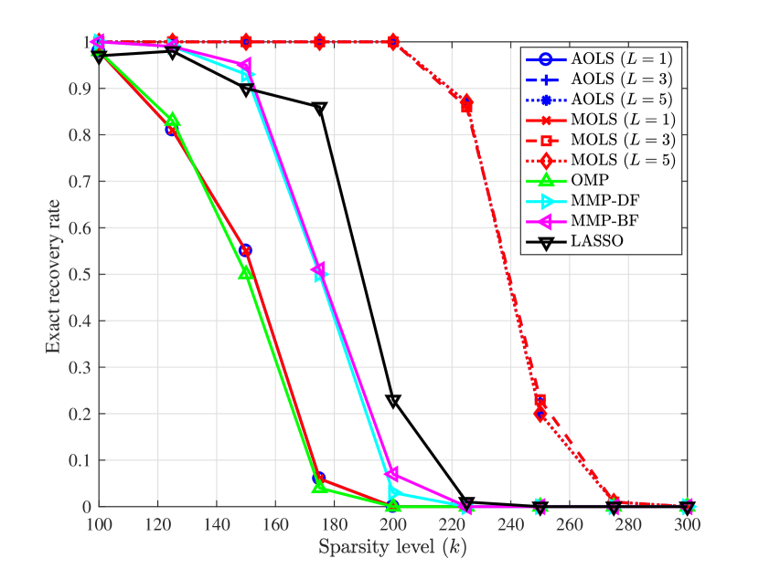
(a) $T=0$

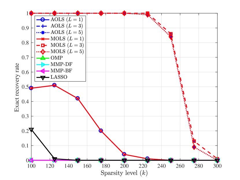
(b) $T=0.5$

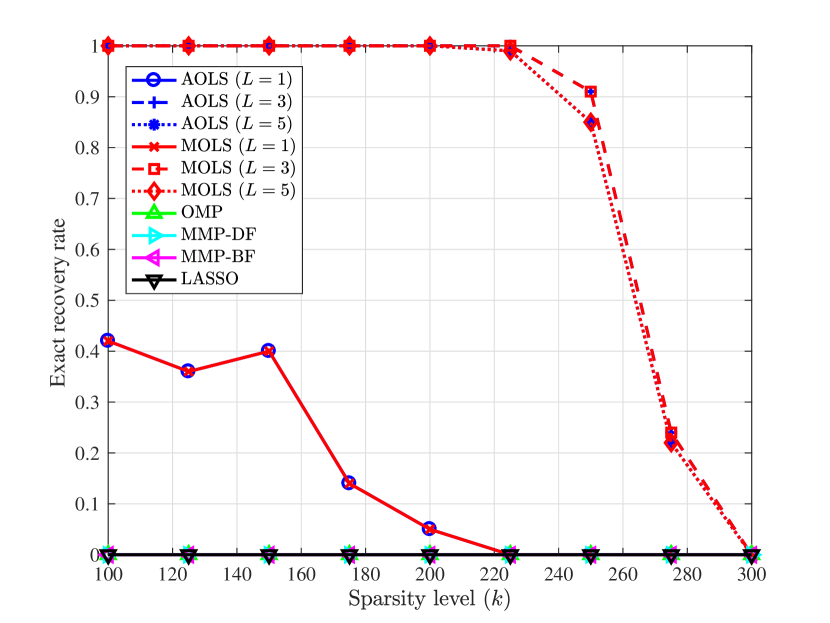
(c) $T=1$

(d) $T=10$

Fig. 4: Exact recovery rate comparison of AOLS, MOLS, OMP, MMP-DP, MMP-BP, and LASSO for $n=512$, $m=1024$, and $k$ non-zero components of ${\mathbf{x}}$ uniformly drawn from ${\cal N}(0,1)$ distribution.

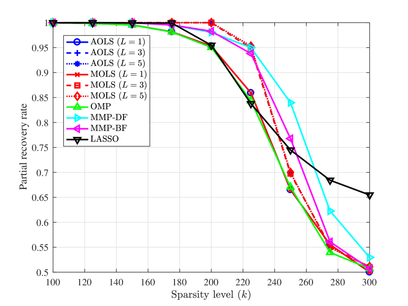
(a) $T=0$

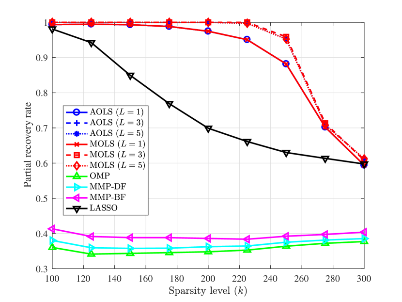
(b) $T=0.5$

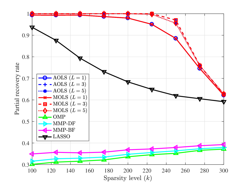
(c) $T=1$

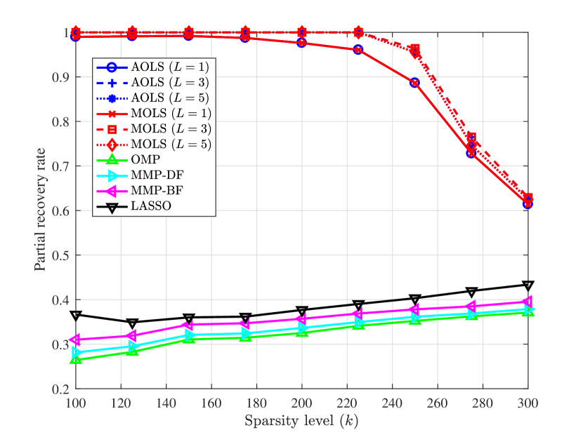
(d) $T=10$

Fig. 5: Partial recovery rate comparison of AOLS, MOLS, OMP, MMP-DP, MMP-BP, and LASSO for $n=512$, $m=1024$, and $k$ non-zero components of ${\mathbf{x}}$ uniformly drawn from ${\cal N}(0,1)$ distribution.

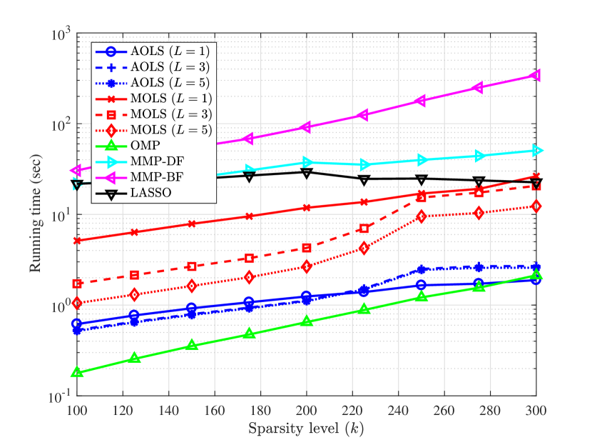
(a) $T=0$

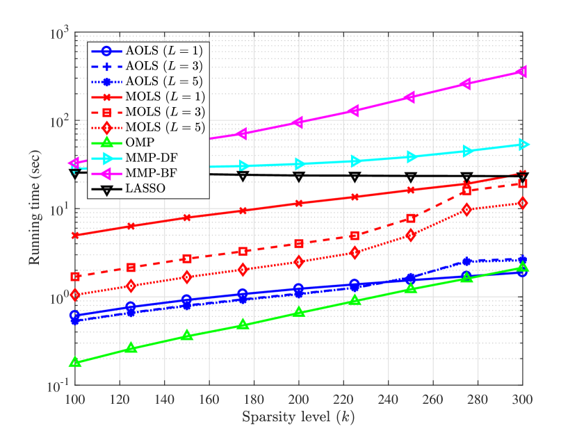
(b) $T=0.5$

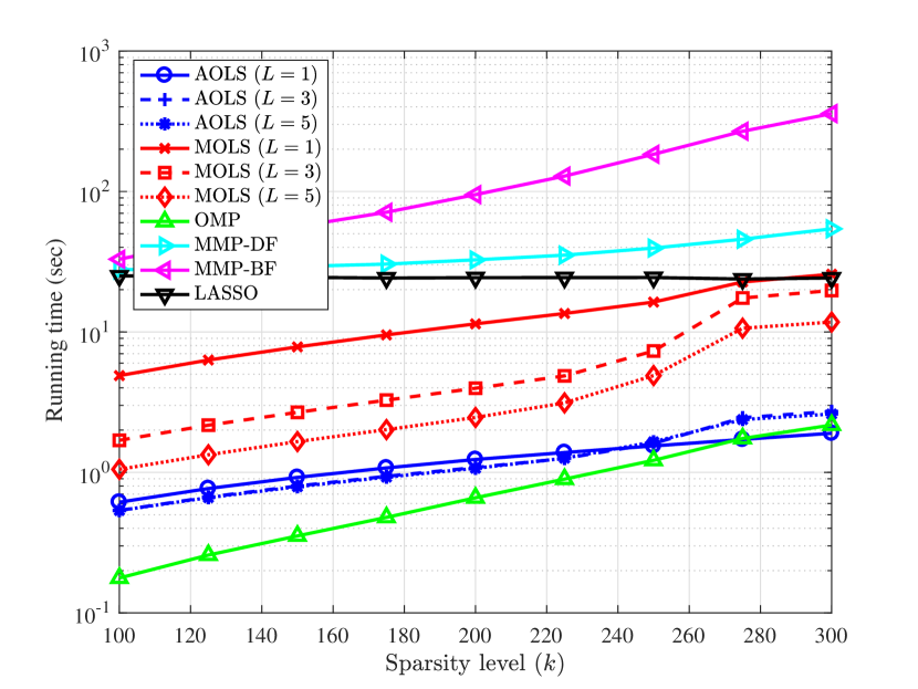
(c) $T=1$

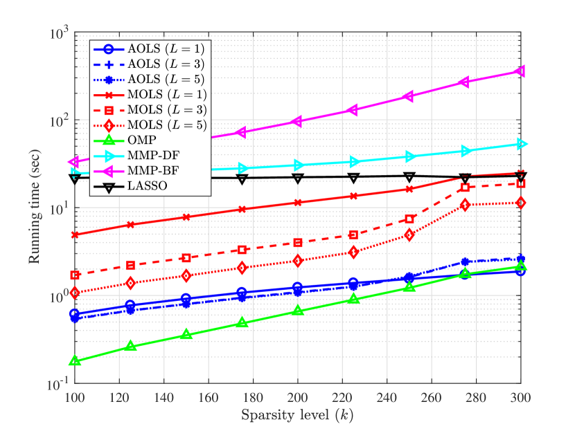
(d) $T=10$

Fig. 6: A comparison of AOLS, MOLS, OMP, MMP-DP, MMP-BP, and LASSO for $n=512$, $m=1024$, and $k$ non-zero components of ${\mathbf{x}}$ uniformly drawn from the ${\cal N}(0,1)$ distribution.

To evaluate performance of the AOLS algorithm, we compare it with that of five state-of-the-art sparse recovery algorithms as a function of the sparsity level $k$. In particular, we considered OMP [13], Least Absolute Shrinkage and Selection Operator (LASSO) [45, 10], MOLS [33] with $L=1,3,5$, depth-first and breath-first multipath matching pursiut [35] (refered to as MMP-DF and MMP-BP, respectively). It is shown in [33, 35] that MOLS, MMP-DF, and MMP-BP outperform many of the sparse recovery algorithms, including OLS [14], OMP [13], GOMP [17], StOMP [16], and BP [10]. Therefore, to demonstrate performance and uniqueness of AOLS with respect to other sparse recovery methods, we compare it to these three schemes. We also include performance of OMP and LASSO as baselines.

For MOLS, MMP-DF, and MMP-BF we used the MATLAB implementations provided by the authors of [33, 35]. As typically done in benchmarking tests [46, 17], we used CVX [47, 48] to implement the LASSO algorithm. We explored various values of $L$ (specifically, $L=1,3,5$) to better understand its effect on the performance of AOLS. The stopping threshold for AOLS, MMP-DF, OMP, MOLS, and LASSO was set to $10^{-13}$ (MMP-BF, a breadth-first algorithm, does not use a stopping threshold).

We consider sparse recovery from random measurements in a large-scale setting to fully understand scalability of tested algorithms. To this end, we set $n=512$ and $m=1024$; $k$ changes from $100$ to $300$. The non-zero elements of ${\mathbf{x}}$ – whose locations are chosen uniformly – are independent and identically distributed normal random variables. In order to construct ${\mathbf{A}}$, we consider the so-called hybrid scenario [30] to simulate both correlated and uncorrelated dictionaries. Specifically, we set ${\mathbf{A}}_{\_}j=\frac{{\mathbf{b}}_{\_}j+t_{\_}j\mathbf{1}}{\|{\mathbf{b}}_{\_}j+t_{\_}j\mathbf{1}\|_{\_}2}$ where ${\mathbf{b}}_{\_}j\sim{\cal N}(0,\frac{1}{n})$, $t_{\_}j\sim{\cal U}(0,T)$ with $T\geq 0$, and $\mathbf{1}\in{\mathbb{R}}^{n}$ is the all-one vector. In addition, $\{{\mathbf{b}}_{\_}j\}_{\_}{j=1}^{m}$ and $\{t_{\_}j\}_{\_}{j=1}^{m}$ are statistically independent. Notice that as $T$ increases, the so-called mutual coherence parameter of ${\mathbf{A}}$ increases, resulting in a more correlated coefficient matrix; $T=0$ corresponds to an incoherent ${\mathbf{A}}$. For each scenario, we use Monte Carlo simulations with $100$ independent instances. Performance of each algorithm is characterized by three metrics: (i) Exact Recovery Rate (ERR), defined as the percentage of instances where the support of ${\mathbf{x}}$ is recovered exactly, (ii) Partial Recovery Rate (PRR), measuring the fraction of support which is recovered correctly, and (iii) the running time of the algorithm.

The exact recovery rate, partial recovery rate, and running time comparisons are shown in Fig. 4, Fig. 5, and Fig. 6, respectively. As can be seen from Fig. 4, AOLS and MOLS with $L=3,5$ achieve the best exact recovery rate for various values of $T$. We also observe that as $T$ increases, performance of all schemes, except for AOLS and MOLS, significantly deteriorates. As for the partial recovery rate shown in Fig. 5, for $T=0$ all methods perform similarly. However, AOLS and MOLS are robust to changes in $T$ while other schemes perform poorly for larger values of $T$. Running time comparison results, depicted in Fig. 6, demonstrate that for all scenarios the AOLS algorithm is essentially as fast as OMP, while AOLS is significantly more accurate. We also observe from the figure that AOLS is significantly faster that other schemes. Specifically, for larger values of $k$, AOLS is around 15 times faster than MOLS, while they deliver essentially the same performance.

5.3 Application: sparse subspace clustering

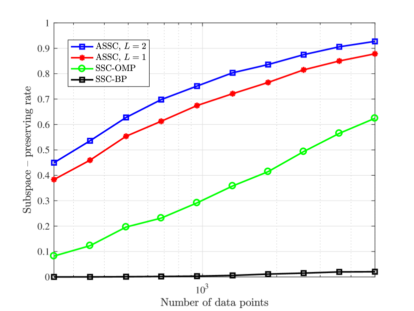
(a) Subspace preserving rate

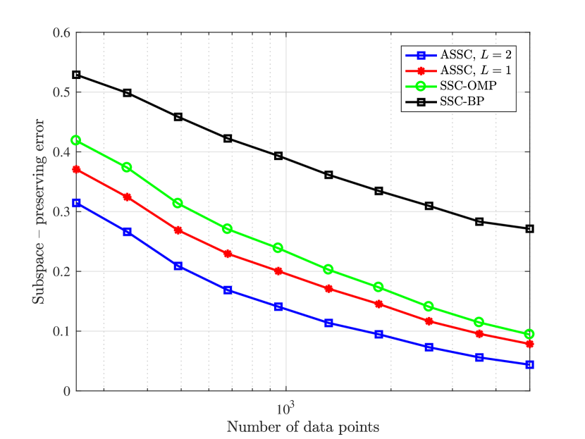
(b) Subspace preserving error

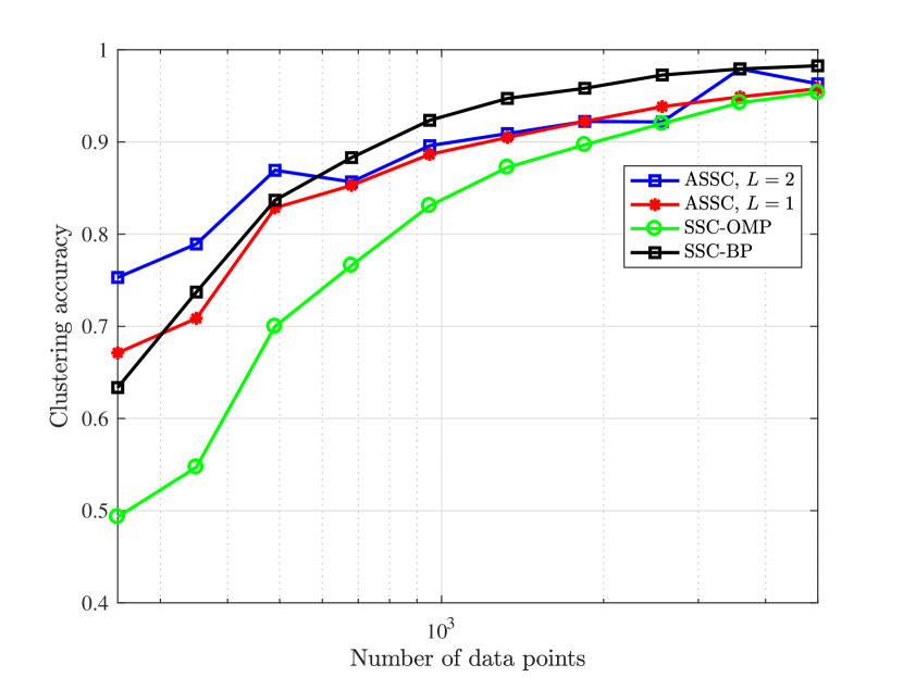
(c) Clustering accuracy

(d) Running time (sec)

Fig. 7: Performance comparison of ASSC, SSC-OMP [39, 3], and SSC-BP [2, 40] on synthetic data with no perturbation. The points are drawn from $5$ subspaces of dimension $6$ in ambient dimension $9$. Each subspace contains the same number of points and the overall number of points is varied from $250$ to $5000$.

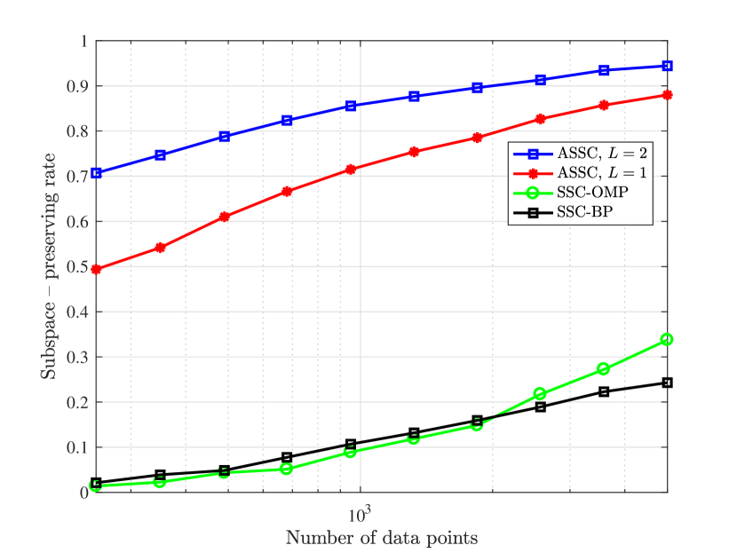
(a) Subspace preserving rate

(b) Subspace preserving error

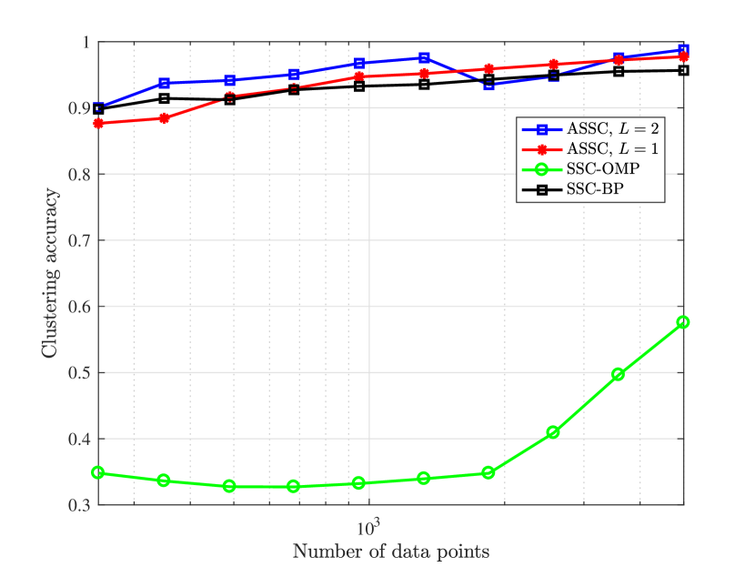
(c) Clustering accuracy

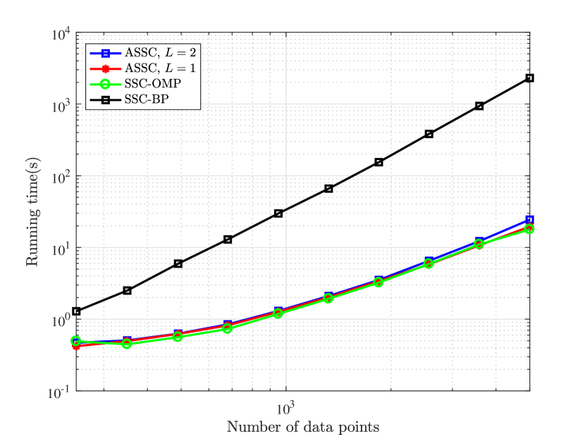
(d) Running time (sec)

Fig. 8: Performance comparison of ASSC, SSC-OMP [39, 3], and SSC-BP [2, 40] on synthetic data with perturbation terms $Q\sim\mathcal{U}(0,1)$. The points are drawn from $5$ subspaces of dimension $6$ in ambient dimension $9$. Each subspace contains the same number of points and the overall number of points is varied from $250$ to $5000$.

Sparse subspace clustering (SSC), which received considerable attention in recent years, relies on sparse signal reconstruction techniques to organize high-dimensional data known to have low-dimensional representation [2]. In particular, in SSC problems we are given matrix ${\mathbf{A}}$ which collects data points ${\mathbf{a}}_{\_}i$ drawn from a union of low-dimensional subspaces, and are interested in partitioning the data according to their subspace membership. State-of-the-art SSC schemes such as SSC-OMP [39, 3] and SSC-BP [2, 40] typically consist of two steps. In the first step, one finds a similarity matrix $\mathbf{W}$ characterizing relative affinity of data points by forming a representation matrix ${\mathbf{C}}$. Once $\mathbf{W}=|{\mathbf{C}}|+|{\mathbf{C}}|^{\top}$ is generated, the second step performs data segmentation by applying spectral clustering [49] on $\mathbf{W}$. Most of the SSC methods rely on the so-called self-expressiveness property of data belonging to a union of subspaces which states that each point in a union of subspaces can be written as a linear combination of other points in the union [2].

In this section, we employ the proposed AOLS algorithm to generate the subspace-preserving similarity matrix $\mathbf{W}$ and empirically compare the resulting SSC performance with that of SSC-OMP [39, 3] and SSC-MP [2, 40]. For SSC-BP, two implementations based on ADMM and interior point methods are available by the authors of [2, 40]. In our simulation studies we use the ADMM implementation of SSC-BP in [2, 40] as it is faster than the interior point method implementation. Our scheme is tested for $L=1$ and $L=2$. We consider the following two scenarios: (1) A random model where the subspaces are with high probability near-independent; and (2) The setting where we used hybrid dictionaries [30] to generate similar data points across different subspaces which in turn implies the independence assumption no longer holds. In both scenarios, we randomly generate $n=5$ subspaces, each of dimension $d=6$, in an ambient space of dimension $D=9$. Each subspace contains $N_{\_}i$ sample points where we vary $N_{\_}i$ from $50$ to $1000$; therefore, the total number of data points, $N=\sum_{\_}{i=1}^{n}N_{\_}i$, is varied from $250$ to $5000$. The results are averaged over $20$ independent instances. For scenario (1), we generate data points by uniformly sampling from the unit sphere. For the second scenario, after sampling a data point we add a perturbation term $Q\mathbf{1}_{\_}D$ where $Q\sim\mathcal{U}(0,1)$.

In addition to comparing the algorithms in terms of their clustering accuracy and running time, we use the following metrics defined in [2, 40] that quantify the subspace preserving property of the representation matrix ${\mathbf{C}}$ returned by each algorithm:

• Subspace preserving rate: The fraction of points whose representations are subspace-preserving.

• Subspace preserving error: The fraction of $\ell_{\_}1$ norms of the representation coefficients associated with points from other subspaces, i.e., $\frac{1}{N}\sum_{\_}{j}{(\sum_{\_}{i\in O}{|{\mathbf{C}}_{\_}{ij}}|/\|{\mathbf{c}}_{\_}j\|_{\_}1)}$ where $O$ represents the set of data points from other subspaces.

The results for the scenario (1) and (2) are illustrated in Fig. 7 and Fig. 8, respectively. As can be seen in Fig. 7, ASSC is nearly as fast as SSC-OMP and orders of magnitude faster than SSC-BP while ASSC achieves better subspace preserving rate, subspace preserving error, and clustering accuracy compared to competing schemes. In the second scenario, we observe that the performance of SSC-OMP is severely deteriorated while ASSC still outperforms both SSC-BP and SSC-OMP in terms of accuracy. Further, similar to the first scenario, running time of ASSC is similar to that of SSC-OMP while both methods are much faster that SSC-BP. As Fig. 7 and Fig. 8 suggest, the ASSC algorithm, especially with $L=2$, outperforms other schemes while essentially being as fast as the SSC-OMP method.

6 Conclusions and Future Work

In this paper, we proposed the Accelerated Orthogonal Least-Squares (AOLS) algorithm, a novel scheme for sparse vector approximation. AOLS, unlike state-of-the art OLS-based schemes such as Multiple Orthogonal Least-Squares (MOLS) [33], relies on a set of expressions which provide computationally efficient recursive updates of the orthogonal projection operator and enable computation of the residual vector by employing only linear equations. Additionally, AOLS allows incorporating $L$ columns in each iteration to further reduce the complexity while achieving improved performance. In our theoretical analysis of AOLS, we showed that for coefficient matrices consisting of entries drawn from a Gaussian distribution, AOLS with high probability recovers $k$-sparse $m$-dimensional signals in at most $k$ iterations from ${\cal O}(k\log\frac{m}{k+L-1})$ noiseless random linear measurements. We extended this result to the scenario where the measurements are perturbed with $\ell_{\_}2$-bounded noise. Specifically, if the non-zero elements of an unknown vector are sufficiently large, ${\cal O}(k\log\frac{m}{k+L-1})$ random linear measurements is sufficient to guarantee recovery with high probability. This asymptotic bound on the required number of measurements is lower than those of the existing OLS-based, OMP-based, and convex relaxation schemes. Our simulation results verify that ${\cal O}\left(k\log\frac{m}{k+L-1}\right)$ measurement is indeed sufficient for sparse reconstruction that is exact with probability arbitrarily close to one. Simulation studies demonstrate that AOLS outperforms all of the current state-of-the-art methods in terms of both accuracy and running time. Furthermore, we considered an application to sparse subspace clustering where we employed AOLS to facilitate efficient clustering of high-dimensional data points lying on the union of low-dimensional subspaces, showing superior performance compared to state-of-the-art OMP-based and BP-based methods [3, 39, 2, 40].

As part of future work, it would be valuable to further extend the analysis carried out in Section 4 to study performance of AOLS for hybrid dictionaries [30]. It is also of interest to analytically characterize performance of the AOLS-based sparse subspace clustering scheme.

Appendices

Appendix A Proof of Lemma 2

The lemma aims to characterize the length of the projection of a random vector onto a low dimensional subspace. In the following argument we show that the distribution of the length of the projected vector is invariant to rotation which in turn enables us to find the projection in a straightforward manner.

Recall that ${\mathbf{P}}_{\_}k$ is an orthogonal projection operator for a $k$-dimensional subspace ${\cal L}_{\_}k$ spanned by the columns of ${\mathbf{A}}_{\_}k$. Let ${\cal B}=\{{{\mathbf{b}}_{\_}1},\dots,{{\mathbf{b}}_{\_}k}\}$ denote an orthonormal basis for ${\cal L}_{\_}k$. There exist a rotation operator $\cal R$ such that ${\cal R}\left({\cal B}\right)=\{{\mathbf{e}_{\_}1},\dots,{\mathbf{e}_{\_}k}\}$, where $\mathbf{e}_{\_}i$ is the $i\textsuperscript{th}$ standard unit vector. Let ${\mathbf{u}}\sim{\cal N}(0,1/n)$. Since a multivariate Gaussian distribution is spherically symmetric [50], distribution of ${\mathbf{u}}$ remains unchanged under rotation, i.e., ${\cal R}\left({\mathbf{u}}\right)\sim{\cal N}(0,1/n)$. Therefore, it holds that $\operatorname{\mathbb{E}}\left\lVert{\cal R}\left({\mathbf{u}}\right)\right\rVert_{\_}2=\operatorname{\mathbb{E}}\left\lVert{\mathbf{u}}\right\rVert_{\_}2$. In addition, since after rotation $\{{\mathbf{e}_{\_}1},\dots,{\mathbf{e}_{\_}k}\}$ is a basis for the rotation of ${\cal L}_{\_}k$, $\left\lVert{\mathbf{P}}_{\_}k{\mathbf{u}}\right\rVert_{\_}2$ has the same distribution as the length of a vector consisting of the first $k$ components of ${\cal R}\left({\mathbf{u}}\right)$. It then follows from the i.i.d. assumption and linearity of expectation that $\operatorname{\mathbb{E}}\left\lVert{\mathbf{P}}_{\_}k{\mathbf{u}}\right\rVert_{\_}2^{2}=\frac{k}{n}\operatorname{\mathbb{E}}\left\lVert{\mathbf{u}}\right\rVert_{\_}2^{2}=\frac{k}{n}$.

We now prove the statement in the second part of the lemma. Let ${\mathbf{u}}_{\_}k^{\cal R}$ be the vector collecting the first $k$ coordinates of ${\cal R}({\mathbf{u}})$. The above argument implies $\left\lVert{\mathbf{P}}_{\_}k{\mathbf{u}}\right\rVert_{\_}2^{2}$ has the same distribution as $\left\lVert{\mathbf{u}}_{\_}k^{\cal R}\right\rVert_{\_}2^{2}$. In addition, $n\left\lVert{\mathbf{u}}_{\_}k^{\cal R}\right\rVert_{\_}2^{2}$ is distributed as $\chi^{2}_{\_}k$ because of the spherical symmetry property of ${\mathbf{u}}$. Let $\lambda>0$; we will specify the value of $\lambda$ shortly. Now,

$$\Pr\{\left\lVert{\mathbf{P}}_{\_}k{\mathbf{u}}\right\rVert_{\_}2^{2}\leq(1-\epsilon)\frac{k}{n}\} =\Pr\{n\left\lVert{\mathbf{u}}_{\_}k^{\cal R}\right\rVert_{\_}2^{2}\leq(1-\epsilon)k\}$$ (36)

$$=\Pr\{-\frac{\lambda}{2}n\left\lVert{\mathbf{u}}_{\_}k^{\cal R}\right\rVert_{\_}2^{2}\geq-\frac{\lambda k(1-\epsilon)}{2}\}$$

$$=\Pr\{e^{-\frac{\lambda}{2}n\left\lVert{\mathbf{u}}_{\_}k^{\cal R}\right\rVert_{\_}2^{2}}\geq e^{-\frac{\lambda k(1-\epsilon)}{2}}\}$$

$$\stackrel{{\scriptstyle(a)}}{{\leq}}e^{\frac{\lambda k(1-\epsilon)}{2}}\operatorname{\mathbb{E}}\{e^{-\frac{\lambda}{2}n\left\lVert{\mathbf{u}}_{\_}k^{\cal R}\right\rVert_{\_}2^{2}}\}$$

$$\stackrel{{\scriptstyle(b)}}{{=}}e^{\frac{\lambda k(1-\epsilon)}{2}}(1+\lambda)^{\frac{-k}{2}}$$

where (a) follows from the Markov inequality and (b) is due to the definition of the Moment Generating Function (MGF) for $\chi^{2}_{\_}k$-distribution. Now, let $\lambda=\frac{\epsilon}{1-\epsilon}$. It follows that

$$\Pr\{\left\lVert{\mathbf{P}}_{\_}k{\mathbf{u}}\right\rVert_{\_}2^{2}\leq(1-\epsilon)\frac{k}{n}\}\leq e^{\frac{\lambda k(1-\epsilon)}{2}}(1-\epsilon)^{\frac{k}{2}}=e^{\frac{k}{2}(\epsilon+\log(1-\epsilon))}\leq e^{\frac{-k\epsilon^{2}}{4}}$$ (37)

where in the last inequality we used the fact that $\log(1-\epsilon)\leq-\epsilon-\frac{\epsilon^{2}}{2}$. Following the same line of argument, one can show that

$$\Pr\{\left\lVert{\mathbf{P}}_{\_}k{\mathbf{u}}\right\rVert_{\_}2^{2}\geq(1+\epsilon)\frac{k}{n}\}\leq e^{-k(\frac{\epsilon^{2}}{4}-\frac{\epsilon^{3}}{6})}.$$ (38)

The combination of (37) and (38) using Boole’s inequality leads to the stated result.

Appendix B Proof of Theorem 6

Here we follow the outline of the proof of Theorem 5. Note that, in the presence of noise, $\bar{{\mathbf{A}}}^{\top}{\mathbf{r}}_{\_}i$ in (25) has at most $k$ nonzero entries. After a straightforward modification of (26), we obtain

$$\rho({\mathbf{r}}_{\_}i)\leq\frac{\sqrt{k}}{c_{\_}1(\epsilon)}|\mathcal{P}(\widetilde{{\mathbf{A}}}^{\top}{\mathbf{r}}_{\_}i)_{\_}{m-k-L+1}|.$$ (39)

The most important difference between the noisy and noiseless scenarios is that ${\mathbf{r}}_{\_}i$ in the latter does not belong to the range of $\bar{{\mathbf{A}}}$; therefore, further restrictions are needed to ensure that $\{\widetilde{{\mathbf{r}}}_{\_}i\}_{\_}{i=0}^{k-1}$ remains bounded. To this end, we investigate lower bounds on $\|\bar{{\mathbf{A}}}^{\top}{\mathbf{r}}_{\_}i\|_{\_}2$ and upper bounds on $\|\widetilde{{\mathbf{r}}}_{\_}i\|_{\_}2$. Recall that in the $i\textsuperscript{th}$ iteration

$${\mathbf{r}}_{\_}i={\mathbf{P}}_{\_}i^{\bot}{\mathbf{y}}={\mathbf{P}}_{\_}i^{\bot}\left(\bar{{\mathbf{A}}}\bar{{\mathbf{x}}}+{\boldsymbol{\nu}}\right),$$ (40)

where $\bar{{\mathbf{x}}}\in{\mathbb{R}}^{k}$ is a subvector of ${\mathbf{x}}$ that collects nonzero components of ${\mathbf{x}}$. We can write ${\boldsymbol{\nu}}$ equivalently as

$${\boldsymbol{\nu}}=\bar{{\mathbf{A}}}{\mathbf{w}}+{\boldsymbol{\nu}}^{\bot},$$ (41)

where ${\boldsymbol{\nu}}^{\bot}={\mathbf{P}}_{\_}k^{\bot}{\boldsymbol{\nu}}$ is the projection of ${\boldsymbol{\nu}}$ onto the orthogonal complement of the subspace spanned by the columns of ${\mathbf{A}}$ corresponding to nonzero entries of ${\mathbf{x}}$, and ${\mathbf{w}}=\bar{{\mathbf{A}}}^{\dagger}{\boldsymbol{\nu}}$. Substituting (41) into (40) and noting that ${\mathbf{P}}_{\_}i^{\bot}{\mathbf{a}}=0$ if ${\mathbf{a}}$ is selected in previous iterations as well as observing that ${\cal L}_{\_}i\subset{\cal L}_{\_}k$, we obtain

$${\mathbf{r}}_{\_}i={\boldsymbol{\nu}}^{\bot}+{\mathbf{P}}_{\_}i^{\bot}\bar{{\mathbf{A}}}_{\_}{i^{c}}{\mathbf{c}}_{\_}{i^{c}},$$ (42)

where ${\mathbf{c}}=\bar{{\mathbf{x}}}+{\mathbf{w}}$ and subscript $i^{c}$ denotes the set of correct columns that have not yet been selected. Evidently, (42) demonstrates that ${\mathbf{r}}_{\_}i$ can be written as a sum of orthogonal terms. Therefore,

$$\|{\mathbf{r}}_{\_}i\|_{\_}2^{2}=\|{\boldsymbol{\nu}}^{\bot}\|_{\_}2^{2}+\|{\mathbf{P}}_{\_}i^{\bot}\bar{{\mathbf{A}}}_{\_}{i^{c}}{\mathbf{c}}_{\_}{i^{c}}\|_{\_}2^{2}.$$ (43)

Applying (42) yields

$$\|\bar{{\mathbf{A}}}^{\top}{\mathbf{r}}_{\_}i\|_{\_}2 =\|\bar{{\mathbf{A}}}^{\top}\left({\boldsymbol{\nu}}^{\bot}+{\mathbf{P}}_{\_}i^{\bot}\bar{{\mathbf{A}}}_{\_}{i^{c}}{\mathbf{c}}_{\_}{i^{c}}\right)\|_{\_}2$$ (44)

$$\stackrel{{\scriptstyle(a)}}{{=}}\|\bar{{\mathbf{A}}}^{\top}{\boldsymbol{\nu}}^{\bot}+\bar{{\mathbf{A}}}_{\_}{i^{c}}^{\top}{\mathbf{P}}_{\_}i^{\bot}\bar{{\mathbf{A}}}_{\_}{i^{c}}{\mathbf{c}}_{\_}{i^{c}}\|_{\_}2$$

$$\stackrel{{\scriptstyle(b)}}{{=}}\|\bar{{\mathbf{A}}}_{\_}{i^{c}}^{\top}{\mathbf{P}}_{\_}i^{\bot}\bar{{\mathbf{A}}}_{\_}{i^{c}}{\mathbf{c}}_{\_}{i^{c}}\|_{\_}2$$

$$\stackrel{{\scriptstyle(c)}}{{\geq}}\sigma_{\_}{\min}^{2}(\bar{{\mathbf{A}}})\|{\mathbf{c}}_{\_}{i^{c}}\|_{\_}2,$$

where ($a$) holds because ${\mathbf{P}}_{\_}i^{\bot}$ projects onto the orthogonal complement of the space spanned by the columns of $\bar{{\mathbf{A}}}_{\_}i$, ($b$) follows from the fact that columns of $\bar{{\mathbf{A}}}$ and ${\boldsymbol{\nu}}^{\bot}$ lie in orthogonal subspaces, and ($c$) follows from Lemma 3 and the fact that ${\mathbf{P}}_{\_}i^{\bot}$ is a projection matrix.

We now bound the norm of $\widetilde{{\mathbf{r}}}_{\_}i$. Substitute (43) and (44) in the definition of $\widetilde{{\mathbf{r}}}_{\_}i$ to arrive at

$$\|\widetilde{{\mathbf{r}}}_{\_}i\|_{\_}2 \leq\frac{\left[\|{\boldsymbol{\nu}}^{\bot}\|_{\_}2^{2}+\|{\mathbf{P}}_{\_}i^{\bot}\bar{{\mathbf{A}}}_{\_}{i^{c}}{\mathbf{c}}_{\_}{i^{c}}\|_{\_}2^{2}\right]^{\frac{1}{2}}}{\sigma_{\_}{\min}^{2}(\bar{{\mathbf{A}}})\|{\mathbf{c}}_{\_}{i^{c}}\|_{\_}2}$$ (45)

$$\stackrel{{\scriptstyle(a)}}{{\leq}}\frac{\left[\|{\boldsymbol{\nu}}^{\bot}\|_{\_}2^{2}+\sigma_{\_}{\max}^{2}(\bar{{\mathbf{A}}})\|{\mathbf{c}}_{\_}{i^{c}}\|_{\_}2^{2}\right]^{\frac{1}{2}}}{\sigma_{\_}{\min}^{2}(\bar{{\mathbf{A}}})\|{\mathbf{c}}_{\_}{i^{c}}\|_{\_}2}$$

$$=\frac{\left[\|{\boldsymbol{\nu}}^{\bot}\|_{\_}2^{2}/\|{\mathbf{c}}_{\_}{i^{c}}\|_{\_}2^{2}+\sigma_{\_}{\max}^{2}(\bar{{\mathbf{A}}})\right]^{\frac{1}{2}}}{\sigma_{\_}{\min}^{2}(\bar{{\mathbf{A}}})}$$

where ($a$) follows from Lemma 3 and the fact that ${\mathbf{P}}_{\_}i^{\bot}$ is a projection matrix. In addition,

$$\|{\boldsymbol{\nu}}^{\bot}\|_{\_}2=\|{\mathbf{P}}_{\_}k^{\bot}{\boldsymbol{\nu}}\|_{\_}2\leq\|{\boldsymbol{\nu}}\|_{\_}2\leq\epsilon_{\_}{{\boldsymbol{\nu}}}.$$ (46)

Defining ${\mathbf{x}}_{\_}{\min}=\min_{\_}{j}{|\bar{{\mathbf{x}}}_{\_}j|}$ and ${\mathbf{c}}_{\_}{\min}=\min_{\_}{j}{|{\mathbf{c}}_{\_}j|}$, it is straightforward to see that

$${\mathbf{c}}_{\_}{\min}\geq{\mathbf{x}}_{\_}{\min}-\|{\mathbf{w}}\|_{\_}2.$$ (47)

Moreover, we impose ${\mathbf{x}}_{\_}{\min}\geq(1+\delta)\|{\mathbf{w}}\|_{\_}2$. Therefore,

$$\|{\mathbf{c}}_{\_}{i^{c}}\|_{\_}2^{2} \geq(k-i){\mathbf{c}}_{\_}{\min}^{2}$$ (48)

$$\geq(k-i)\left({\mathbf{x}}_{\_}{\min}-\|{\mathbf{w}}\|_{\_}2\right)^{2}$$

$$=(k-i)({\mathbf{x}}_{\_}{\min}-\|\bar{{\mathbf{A}}}^{\dagger}{\boldsymbol{\nu}}\|_{\_}2)^{2}$$

$$\geq(k-i)({\mathbf{x}}_{\_}{\min}-\sigma_{\_}{\max}(\bar{{\mathbf{A}}}^{\dagger})\|{\boldsymbol{\nu}}\|_{\_}2)^{2}$$

$$=(k-i)({\mathbf{x}}_{\_}{\min}-\sigma_{\_}{\min}(\bar{{\mathbf{A}}})\epsilon_{\_}{{\boldsymbol{\nu}}})^{2}.$$

Combining (45), (46), and (48) implies that

$$\|\widetilde{{\mathbf{r}}}_{\_}i\|_{\_}2 \leq\frac{\left[\frac{\epsilon_{\_}{{\boldsymbol{\nu}}}^{2}}{(k-i)({\mathbf{x}}_{\_}{\min}-\sigma_{\_}{\min}(\bar{{\mathbf{A}}})\epsilon_{\_}{{\boldsymbol{\nu}}})^{2}}+\sigma_{\_}{\max}^{2}(\bar{{\mathbf{A}}})\right]^{\frac{1}{2}}}{\sigma_{\_}{\min}^{2}(\bar{{\mathbf{A}}})}$$ (49)

$$\leq\frac{\left[\frac{\epsilon_{\_}{{\boldsymbol{\nu}}}^{2}}{(k-i)({\mathbf{x}}_{\_}{\min}-(1+\delta)\epsilon_{\_}{{\boldsymbol{\nu}}})^{2}}+(1+\delta)^{2}\right]^{\frac{1}{2}}}{(1-\delta)^{2}}$$

with probability exceeding $p_{\_}2$. Thus, imposing the constraint

$${\mathbf{x}}_{\_}{\min}\geq(1+\delta+t)\epsilon_{\_}{{\boldsymbol{\nu}}}$$ (50)

where $t>0$ establishes

$$\|\widetilde{{\mathbf{r}}}_{\_}i\|_{\_}2\leq\frac{\left[\frac{1}{(k-i)t^{2}}+(1+\delta)^{2}\right]^{\frac{1}{2}}}{(1-\delta)^{2}}.$$ (51)

By following the steps of the proof of Theorem 5 and exploiting independence of the columns of $\widetilde{{\mathbf{A}}}$, we arrive at

$$\Pr\{\Sigma\}\geq p_{\_}1p_{\_}2\Pr\{\max_{\_}{0\leq i<k}{\left|\widetilde{{\mathbf{a}}}_{\_}{o_{\_}1}^{\top}\widetilde{{\mathbf{r}}}_{\_}i\right|}<\frac{c_{\_}1(\epsilon)}{\sqrt{k}}\}^{m-k-L+1}.$$ (52)

Recall that $\{\widetilde{{\mathbf{r}}}_{\_}i\}_{\_}{i=0}^{k-1}$ are statistically independent of $\widetilde{{\mathbf{A}}}$ and that with probability higher than $p_{\_}2$ they are bounded. By using Boole’s for the random variable $X_{\_}{i}=\widetilde{{\mathbf{a}}}_{\_}{o_{\_}1}^{\top}\widetilde{{\mathbf{r}}}_{\_}i$ we obtain

$$\Pr\{\max_{\_}{0\leq i<k}{\left|X_{\_}{i}\right|<\frac{c_{\_}1(\epsilon)}{\sqrt{k}}}\}\geq 1-\sum_{\_}{i=0}^{k-1}e^{-\frac{nc_{\_}1(\epsilon)^{2}(1-\delta)^{4}}{k\left[\frac{1}{(k-i)t^{2}}+(1+\delta)^{2}\right]}}.$$ (53)

Let us denote

$$p_{\_}3=\left(1-\sum_{\_}{i=0}^{k-1}e^{-\frac{nc_{\_}1(\epsilon)^{2}(1-\delta)^{4}}{k\left[\frac{1}{(k-i)t^{2}}+(1+\delta)^{2}\right]}}\right)^{m-k-L+1}.$$ (54)

Then from (52) and (53) follows that $\Pr\{\Sigma\}\geq p_{\_}1p_{\_}2p_{\_}3$, which completes the proof.

Remark 4: Note that in the absence of noise the first term in the numerator of (51) vanishes, leading to $\|\widetilde{{\mathbf{r}}}_{\_}i\|_{\_}2\leq\frac{1}{1-\delta}+\frac{2\delta}{(1-\delta)^{2}}$. A comparison with the proof of Theorem 5 suggests that the term $\frac{2\delta}{(1-\delta)^{2}}$ is a modification which stems from the presence of noise.

References

- [1] D. L. Donoho, “Compressed sensing,” IEEE Transactions on Information Theory, vol. 52, no. 4, pp. 1289–1306, Apr. 2006.
- [2] E. Elhamifar and R. Vidal, “Sparse subspace clustering,” in Proceedings of the IEEE Conference on Computer Vision and Pattern Recognition (CVPR), pp. 2790–2797, IEEE, 2009.
- [3] C. You, D. Robinson, and R. Vidal, “Scalable sparse subspace clustering by orthogonal matching pursuit,” in in Proceedings of the IEEE Conference on Computer Vision and Pattern Recognition (CVPR), pp. 3918–3927, 2016.
- [4] C. Carbonelli, S. Vedantam, and U. Mitra, “Sparse channel estimation with zero tap detection,” IEEE Transactions on Wireless Communications, vol. 6, no. 5, pp. 1743–1763, May 2007.
- [5] S. Barik and H. Vikalo, “Sparsity-aware sphere decoding: Algorithms and complexity analysis,” IEEE Transactions on Signal Processing, vol. 62, no. 9, pp. 2212–2225, May 2014.
- [6] F. Parvaresh, H. Vikalo, S. Misra, and B. Hassibi, “Recovering sparse signals using sparse measurement matrices in compressed DNA microarrays,” IEEE Journal of Selected Topics in Signal Processing, vol. 2, no. 3, pp. 275–285, June 2008.
- [7] M. Lustig, D. Donoho, and J. M. Pauly, “Sparse MRI: The application of compressed sensing for rapid MR imaging,” Magnetic resonance in medicine, vol. 58, no. 6, pp. 1182–1195, Dec. 2007.
- [8] M. Elad, M. A. Figueiredo, and Y. Ma, “On the role of sparse and redundant representations in image processing,” Proceedings of the IEEE, vol. 98, no. 6, pp. 972–982, June 2010.
- [9] M. E. Tipping, “Sparse Bayesian learning and the relevance vector machine,” The Journal of Machine Learning Research, vol. 1, pp. 211–244, June 2001.
- [10] E. J. Candes and T. Tao, “Decoding by linear programming,” IEEE Transactions on Information Theory, vol. 51, no. 12, pp. 4203–4215, Dec. 2005.
- [11] A. Beck and M. Teboulle, “A fast iterative shrinkage-thresholding algorithm for linear inverse problems,” SIAM Journal on Imaging Sciences, vol. 2, no. 1, pp. 183–202, Mar. 2009.
- [12] S. Boyd, N. Parikh, E. Chu, B. Peleato, and J. Eckstein, “Distributed optimization and statistical learning via the alternating direction method of multipliers,” Foundations and Trends® in Machine Learning, vol. 3, no. 1, pp. 1–122, Jan. 2011.
- [13] Y. C. Pati, R. Rezaiifar, and P. Krishnaprasad, “Orthogonal matching pursuit: Recursive function approximation with applications to wavelet decomposition,” in Conference Record of The Twenty-Seventh Asilomar Conference on Signals, Systems and Computers, pp. 40–44, IEEE, 1993.
- [14] S. Chen, S. A. Billings, and W. Luo, “Orthogonal least squares methods and their application to non-linear system identification,” International Journal of Control, vol. 50, no. 5, pp. 1873–1896, Nov. 1989.
- [15] B. K. Natarajan, “Sparse approximate solutions to linear systems,” SIAM journal on computing, vol. 24, no. 2, pp. 227–234, Apr. 1995.
- [16] D. L. Donoho, Y. Tsaig, I. Drori, and J.-L. Starck, “Sparse solution of underdetermined systems of linear equations by stagewise orthogonal matching pursuit,” IEEE Transactions on Information Theory, vol. 58, no. 2, pp. 1094–1121, Feb. 2012.
- [17] J. Wang, S. Kwon, and B. Shim, “Generalized orthogonal matching pursuit,” IEEE Transactions on Signal Processing, vol. 60, no. 12, pp. 6202–6216, Dec. 2012.
- [18] D. Needell and J. A. Tropp, “CoSaMP: Iterative signal recovery from incomplete and inaccurate samples,” Applied and Computational Harmonic Analysis, vol. 26, no. 3, pp. 301–321, May 2009.
- [19] T. Zhang, “Sparse recovery with orthogonal matching pursuit under RIP,” IEEE Transactions on Information Theory, vol. 57, no. 9, pp. 6215–6221, Sep. 2011.
- [20] M. A. Davenport and M. B. Wakin, “Analysis of orthogonal matching pursuit using the restricted isometry property,” IEEE Transactions on Information Theory, vol. 56, no. 9, pp. 4395–4401, Sep. 2010.
- [21] Q. Mo and Y. Shen, “A remark on the restricted isometry property in orthogonal matching pursuit,” IEEE Transactions on Information Theory, vol. 58, no. 6, pp. 3654–3656, June. 2012.
- [22] J. A. Tropp, “Greed is good: Algorithmic results for sparse approximation,” IEEE Transactions on Information Theory, vol. 50, no. 10, pp. 2231–2242, Oct. 2004.
- [23] T. T. Cai and L. Wang, “Orthogonal matching pursuit for sparse signal recovery with noise,” IEEE Transactions on Information Theory, vol. 57, no. 7, pp. 4680–4688, July 2011.
- [24] T. Zhang, “On the consistency of feature selection using greedy least squares regression,” Journal of Machine Learning Research, vol. 10, pp. 555–568, Mar. 2009.
- [25] J. A. Tropp and A. C. Gilbert, “Signal recovery from random measurements via orthogonal matching pursuit,” IEEE Transactions on Information Theory, vol. 53, no. 12, pp. 4655–4666, Dec. 2007.
- [26] A. K. Fletcher and S. Rangan, “Orthogonal matching pursuit: A Brownian motion analysis,” IEEE Transactions on Signal Processing, vol. 60, no. 3, pp. 1010–1021, Mar. 2012.
- [27] S. Rangan and A. K. Fletcher, “Orthogonal matching pursuit from noisy random measurements: A new analysis,” in Proceedings of the Advances in Neural Information Processing Systems (NIPS), pp. 540–548, 2009.
- [28] S. Foucart, “Stability and robustness of weak orthogonal matching pursuits,” in Recent advances in harmonic analysis and applications, pp. 395–405, Springer, 2012.
- [29] J. Wang, S. Kwon, P. Li, and B. Shim, “Recovery of sparse signals via generalized orthogonal matching pursuit: A new analysis,” IEEE Transactions on Signal Processing, vol. 64, no. 4, pp. 1076–1089, Feb. 2016.
- [30] C. Soussen, R. Gribonval, J. Idier, and C. Herzet, “Joint k-step analysis of orthogonal matching pursuit and orthogonal least squares,” IEEE Transactions on Information Theory, vol. 59, no. 5, pp. 3158–3174, May 2013.
- [31] C. Herzet, A. Drémeau, and C. Soussen, “Relaxed recovery conditions for OMP/OLS by exploiting both coherence and decay,” IEEE Transactions on Information Theory, vol. 62, no. 1, pp. 459–470, Jan. 2016.
- [32] C. Herzet, C. Soussen, J. Idier, and R. Gribonval, “Exact recovery conditions for sparse representations with partial support information,” IEEE Transactions on Information Theory, vol. 59, no. 11, pp. 7509–7524, Nov. 2013.
- [33] J. Wang and P. Li, “Recovery of sparse signals using multiple orthogonal least squares,” IEEE Transactions on Signal Processing, vol. 65, no. 8, pp. 2049–2062, Apr. 2017.
- [34] N. B. Karahanoglu and H. Erdogan, “A* orthogonal matching pursuit: Best-first search for compressed sensing signal recovery,” Digital Signal Processing, vol. 22, no. 4, pp. 555–568, Mar. 2012.
- [35] S. Kwon, J. Wang, and B. Shim, “Multipath matching pursuit,” IEEE Transactions on Information Theory, vol. 60, no. 5, pp. 2986–3001, Mar. 2014.
- [36] S. Maymon and Y. C. Eldar, “The Viterbi algorithm for subset selection,” IEEE Signal Processing Letters, vol. 22, no. 5, pp. 524–528, May 2015.
- [37] A. Hashemi and H. Vikalo, “Recovery of sparse signals via branch and bound least-squares,” in Proceedings of IEEE International Conference on Acoustics, Speech, and Signal Processing (ICASSP), pp. 4760–4764.
- [38] E. J. Candès, J. Romberg, and T. Tao, “Robust uncertainty principles: Exact signal reconstruction from highly incomplete frequency information,” IEEE Transactions on Information Theory, vol. 52, no. 2, pp. 489–509, Feb. 2006.
- [39] E. L. Dyer, A. C. Sankaranarayanan, and R. G. Baraniuk, “Greedy feature selection for subspace clustering,” The Journal of Machine Learning Research, vol. 14, no. 1, pp. 2487–2517, 2013.
- [40] E. Elhamifar and R. Vidal, “Sparse subspace clustering: Algorithm, theory, and applications,” IEEE transactions on pattern analysis and machine intelligence, vol. 35, no. 11, pp. 2765–2781, 2013.
- [41] L. Rebollo-Neira and D. Lowe, “Optimized orthogonal matching pursuit approach,” IEEE Signal Processing Letters, vol. 9, no. 4, pp. 137–140, Apr. 2002.
- [42] A. Hashemi and H. Vikalo, “Sparse linear regression via generalized orthogonal least-squares,” in Proceedings of IEEE Global Conference on Signal and Information Processing (GlobalSIP), pp. 1305–1309, IEEE, Dec. 2016.
- [43] G. H. Golub and C. F. Van Loan, Matrix computations, vol. 3. JHU Press, 2012.
- [44] R. Baraniuk, M. Davenport, R. DeVore, and M. Wakin, “A simple proof of the restricted isometry property for random matrices,” Constructive Approximation, vol. 28, no. 3, pp. 253–263, Dec. 2008.
- [45] R. Tibshirani, “Regression shrinkage and selection via the LASSO,” Journal of the Royal Statistical Society. Series B (Methodological), pp. 267–288, Jan. 1996.
- [46] W. Dai and O. Milenkovic, “Subspace pursuit for compressive sensing signal reconstruction,” IEEE Transactions on Information Theory, vol. 55, no. 5, pp. 2230–2249, May 2009.
- [47] M. Grant and S. Boyd, “CVX: MATLAB software for disciplined convex programming, version 2.1.” http://cvxr.com/cvx, Mar. 2014.
- [48] M. Grant and S. Boyd, “Graph implementations for nonsmooth convex programs,” in Recent Advances in Learning and Control (V. Blondel, S. Boyd, and H. Kimura, eds.), Lecture Notes in Control and Information Sciences, pp. 95–110, Springer-Verlag Limited, 2008. http://stanford.edu/~boyd/graph_dcp.html.
- [49] A. Y. Ng, M. I. Jordan, Y. Weiss, et al., “On spectral clustering: Analysis and an algorithm,” in Proceedings of the Advances in Neural Information Processing Systems (NIPS), vol. 14, pp. 849–856, 2001.
- [50] S. Bochner, Lectures on Fourier Integrals, vol. 42. Princeton University Press, 1959.