A Stackelberg Game Perspective on the Conflict Between Machine Learning and Data Obfuscation

Abstract

Data is the new oil; this refrain is repeated extensively in the age of internet tracking, machine learning, and data analytics. As data collection becomes more personal and pervasive, however, public pressure is mounting for privacy protection. In this atmosphere, developers have created applications to add noise to user attributes visible to tracking algorithms. This creates a strategic interaction between trackers and users when incentives to maintain privacy and improve accuracy are misaligned. In this paper, we conceptualize this conflict through an $N+1$-player, augmented Stackelberg game. First a machine learner declares a privacy protection level, and then users respond by choosing their own perturbation amounts. We use the general frameworks of differential privacy and empirical risk minimization to quantify the utility components due to privacy and accuracy, respectively. In equilibrium, each user perturbs her data independently, which leads to a high net loss in accuracy. To remedy this scenario, we show that the learner improves his utility by proactively perturbing the data himself. While other work in this area has studied privacy markets and mechanism design for truthful reporting of user information, we take a different viewpoint by considering both user and learner perturbation.

I Introduction

In the modern digital ecosystem, users leave behind rich trails of behavioral information. On the internet, websites send user data to third-party trackers such as advertising agencies, social networking sites, and data analytic companies [15]. Tracking is not limited, of course, to the internet. The internet of things (IoT) is a phenomenon that refers to the standardization and integration of communications between physical devices in a way that mimics the connection of computers on the internet. IoT devices such as smartwatches include accelerometers, heart rate sensors, and sleep trackers that measure and upload data about users’ physical and medical conditions [21]. Data from these applications data can be used to improve product or service quality or to drive social change. For example, continuous glucose monitors can provide closed-loop blood glucose control for users with diabetes [1, 17]. The smart grid and renewable energy also stand to benefit from developments in networks of sensors and actuators [5].

I-A Privacy in Machine Learning

While these technologies promise positive impacts, they also threaten privacy. Specifically, the IoT involves new threats in the form of information access, because devices may directly collect sensitive information such as health and location data [3]. In addition, the pervasiveness of tracking and the development of analytics have enabled learners to infer habits and physical conditions over time. These inferences may run even to the granularity of “a user’s mood; stress levels; personality type; bipolar disorder; demographics” [18]. These are unprecedented degrees of access to user information. This access has prompted both qualitative and quantitative privacy research.

While several methods have been developed to quantify privacy, we focus on one particular notion in this paper. Proposed by Cynthia Dwork, differential privacy is a mathematical framework which gives probable limits on the disclosure risks that individuals incur by participating in a database [10, 11, 12]. Using DP, learning algorithms can publish a guarantee on the amount of information disclosed: namely, the constant often denoted $\epsilon_{p}.$ Currently, however, there seems to be little incentives for trackers to adopt DP methods.

I-B User Obfuscation Technologies

To remedy this situation, developers have begun to help users perturb data on their own. Finn and Nissenbaum describe two examples: CacheCloak and TrackMeNot [6]. TrackMeNot is a browser extension that generates decoy search queries in order to prevent trackers from assembling accurate profiles of its users [14]. In the realm of IoT, CacheCloak provides a way for users to access location-based services without revealing their exact geographical positions [16]. The app predicts multiple possibilities for the path of a user, and then retrieves location-based information for each path. This means that an adversary tracking the requests is left with many possible paths rather than a unique one. As another example, the browser extension ScareMail adds words relevant to terrorism to every email that a user issues, postulating that wide adoption of this technique would make dragnet surveillance difficult [2]. Apparently, however, such privacy protection involves costs not only for governments but also for the whole population of users.

I-C Learner-User Interaction

This conflict can be studied by an interaction between $N$ users and a machine learner. This data flow in Fig. 1. In general, both the users and the learner could be interested in the privacy and accuracy of the learning outcome. But these incentives are probably not aligned. Hence the interaction is strategic, and aptly studied by game theory.

We model the user-learner interaction as a two-step process in which the learner first announces his perturbation level, and then the users respond by implementing their own perturbation. This is a realistic assumption, since a critical aspect of DP is the ability to publish measurable privacy guarantees. Knowing this protection, users can decide whether to add their own perturbation in order to further protect their information. The dynamic, two-stage nature of this interaction suggests the framework of Stackelberg games [22, 4].

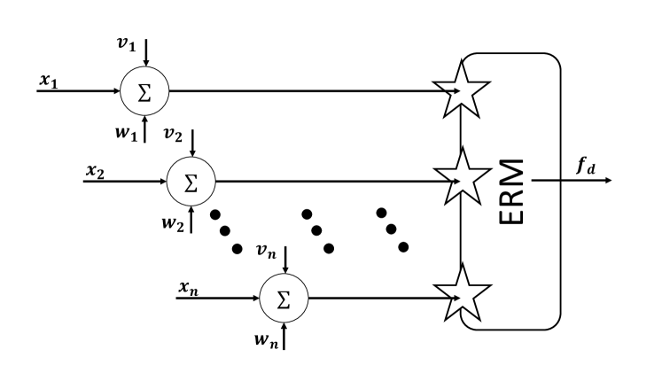
Figure 1: Data flow in the obfuscation-tracking model. Users $1,\ldots,N$ have data $\mathbf{x_{i}}$ with labels $y_{i}.$ Before submitting this data to a classifier, the users add noise $\mathbf{v_{i}}\sim\mathcal{V}_{i},$ and the learner can add noise $\mathbf{w_{i}}\sim\mathcal{W}.$ The classifier is $\mathbf{f_{d}}.$ The stars indicate that the learner is the privacy adversary.

I-D Content and Contributions

In Section II we describe the machine learning technique of Empirical Risk Minimization (ERM) and the framework of DP. Then, in Section III, we employ DP to quantify utility loss due to privacy compromise, and ERM to quantify utility gained through an accurate predictor. In Section IV, we review the solution concept of Stackelberg equilibrium, and we study the equilibrium in Section V. Finally, we discuss the importance of the results in Section VI.

In summary, this paper presents the following contributions:

1. We create a Stackelberg game model to study the conflict between tracking and obfuscation.

2. Our model uses the framework of ERM to quantify accuracy, and DP to quantify privacy loss. These frameworks are sufficiently broad to be used for many different application areas.

3. We find that, while the accuracy levels of all of the users are interdependent, the strategic optimal perturbation level for each user is independent of the perturbation levels of all of the other users (Remark 5).

4. In equilibrium, if the learning algorithm adds sufficient perturbation, it can dissuade the users from obfuscating the data themselves (Remark 8).

5. When the cost of user perturbation is high, protecting user privacy by proactively perturbing is incentive-compatible for the learner (Remark 9).

I-E Related Work

In order to address incentive-compatibility, a vein of research has arisen in privacy markets. In [13], a learner computes a sum of the private bits of a set of users and tries to either maximize accuracy or minimize cost. This paper assumes that users report their data truthfully but can misrepresent their individual valuation of their privacy. Later authors interchanged these assumptions [23]. In work by Chessa et al. [9, 8], users play a multiple person, prior-commitment game, which determines how much they perturb. The present paper differs from all four of these works because it considers the learner as an additional strategic player. Shokri et al. [19] formulate a Stackelberg game for preserving location privacy. In this game, the user is the leader and the learner is the follower. After the user chooses a perturbation strategy, the learner chooses an optimal reconstruction of the user’s location. By contrast, in our model the learner chooses a promised level of privacy protection before the user acts, which makes the learner a Stackelberg leader. Lastly, unlike all of the previous works, our model uses both empirical risk minimization and differential privacy.

II Empirical Risk Minimization and Differential Privacy Models

Consider an interaction between a set of users $i\in S=\left\{1,\ldots,N\right\}$ and a learner $L,$ in which users submit possibly-perturbed data to $L,$ and $L$ releases a statistic or predictor of the data $\mathbf{f_{d}}$ (hereafter, an output). Assume that the data generating process is a random variable $\mathcal{Z}$ with a fixed but unknown distribution. Denote the realized data by $\mathbf{z_{i}}\overset{\text{i.i.d.}}{\sim}\mathcal{Z},\,i\in S.$ Each data point is composed of a feature vector $\mathbf{x_{i}}\in\mathbb{R}^{d}$ and a label $y_{i}\in\left\{-1,1\right\}.$ The goal of the learner $L$ is to predict $y_{i}$ given $\mathbf{x_{i}},$ based on the trained classifier or predictor $\mathbf{f_{d}}.$

In general, privacy loss can occur 1) with respect to $L$, and 2) with respect to the public who observes the output of the ERM. In order to narrow the scope of this paper, we consider information disclosure with respect to $L.$ In addition, information can be leaked through 1) the attributes $\mathbf{x_{i}}$ and 2) the labels $y_{i}.$ We focus on loss due to $\mathbf{x_{i}}$, although analysis using $y_{i}$ would follow many of the same principles.

With the threat of user perturbation, we investigate whether it is advantageous for $L$ to proactively protect the privacy of the users. Thus, we allow $L$ to perturb the submitted data, also before she views it. Assume that $L$ adds noise with the same variance to each data point $\mathbf{x_{i}}.$ For $i\in S,$ $k\in 1,\ldots,d,$ the learner draws $w_{i}^{\left(k\right)}\overset{\text{i.i.d}}{\sim}\mathcal{W},$ where $\mathcal{W}$ is a mean-zero Gaussian random variable with standard deviation $\sigma_{L}.$ Then the user adds noise $v_{i}^{\left(k\right)}\overset{\text{i.i.d.}}{\sim}\mathcal{V}_{i},$ $k\in 1,\ldots,d,$ where $\mathcal{V}_{i}$ is also Gaussian. The perturbed data points are given by $\mathbf{\tilde{x}_{i}}=\mathbf{x_{i}}+\mathbf{v_{i}}+\mathbf{w_{i}},$ $i\in S.$ Figure 1 summarizes this flow of data.

II-A Empirical Risk Minimization

In empirical risk minimization, $L$ calculates a value of output $\mathbf{f_{d}}\in\mathbf{F}$ that minimizes the empirical risk, i.e., the total penalty due to imperfect classification of the realized data. Define the loss function $l\left(\mathbf{\tilde{z}_{i}},\mathbf{f}\right),$ which expresses the penalty due to a single perturbed data point $\mathbf{z_{i}}$ for the output $\mathbf{f}.$ Next let $\Lambda\geq 0$ be a constant and $R\left(\mathbf{f}\right)$ be a regularization term. For $\mathbf{z_{i}}$ in the database $D,$ the total empirical risk is $J\left(\mathbf{f},D\right)=\Lambda R\left(\mathbf{f}\right)+\frac{1}{N}\underset{i}{\sum}l\left(\mathbf{z_{i}},\mathbf{f}\right).$ $L$ obtains $\mathbf{f_{d}}$ given by Eq. 1. Unperturbed data gives the classifier $\mathbf{f^{\dagger}}$ in Eq. 2:

$$\mathbf{f_{d}}=\underset{\mathbf{f}\in\mathbf{F}}{\arg\min}\,\Lambda R\left(\mathbf{f}\right)+\frac{1}{N}\underset{i}{\sum}l\left(\mathbf{\tilde{z}_{i}},\mathbf{f}\right),$$ (1)

$$\mathbf{f^{\dagger}}=\underset{\mathbf{f}\in\mathbf{F}}{\arg\min}\,\Lambda R\left(\mathbf{f}\right)+\frac{1}{N}\underset{i}{\sum}l\left(\mathbf{z_{i}},\mathbf{f}\right).$$ (2)

Expected loss provides a measure of the accuracy of the output of ERM. Let $\mathbf{f^{*}}$ denote the $\mathbf{f}$ which minimizes the expected loss for unperturbed data:

$$\mathbf{f^{*}}=\underset{\mathbf{f}\in\mathbf{F}}{\text{argmin}}\,\mathbb{E}\left\{\Lambda R\left(\mathbf{f}\right)+l\left(\mathcal{Z},\mathbf{f}\right)\right\}.$$ (3)

This forms a reference to which the expected loss of $\mathbf{f_{d}}$ on data $\mathcal{Z}$ can be compared. Let $\epsilon_{g}$ be a positive scalar that bounds the difference in expected loss between the perturbed classifier and the population-optimal classifier. This quantity is given by

$$\mathbb{E}\left\{\Lambda R\left(\mathbf{f_{d}}\right)+l\left(\mathcal{Z},\mathbf{f_{d}}\right)\right\}\leq\mathbb{E}\left\{\Lambda R\left(\mathbf{f^{*}}\right)+l\left(\mathcal{Z},\mathbf{f^{*}}\right)\right\}+\epsilon_{g}.$$ (4)

We use this difference to formulate the accuracy component of utility in Section III.

II-B Differential Privacy

Let $\mathcal{A}\left(*\right)$ denote an algorithm and $D$ denote a database. Let $D^{\prime}$ denote a database that differs from $D$ by only one entry (e.g., the entry of the user under consideration). Let $c$ be some set among all possible sets $C$ in which the output of the algorithm $\mathcal{A}$ may fall. Then Definition 1 quantifies privacy using the framework of DP [7, 10].

Definition 1.

($\epsilon_{p}$-DP) - An algorithm $\mathcal{A}\left(B\right)$ taking values in a set $C$ provides $\left(\epsilon_{p},\delta\right)$-differential privacy if, for all $D,$ $D^{\prime}$ that differ in at most one entry, and for all $c\in C,$

$$\mathbb{P}\left\{\mathcal{A}\left(D\right)\in c\right\}\leq\exp\left(\epsilon_{p}\right)\mathbb{P}\left\{\mathcal{A}\left(D^{\prime}\right)\in c\right\}+\delta.$$ (5)

For a fixed $\delta,$ the degree of randomness determines the privacy level $\epsilon_{p}$. Lower values of $\epsilon_{p}$ correspond to more privacy. That randomness is attained through the noise added in the forms of $\mathcal{V}$ and $\mathcal{W}.$

III Dynamic User-Learner Interaction

We now use the methods for quantification of accuracy and privacy described in Section II as components of utility functions for the users and the learner.

III-A Utility Functions

Let $U_{S}^{i}\left(\sigma_{L},\sigma_{S}^{-i},\sigma_{S}^{i}\right)$ give the utility that each user $i$ receives when the learner chooses perturbation $\sigma_{L},$ user $i$ chooses perturbation level $\sigma_{S}^{i},$ and all of the other users choose perturbation levels $\sigma_{S}^{-i}\triangleq\{\sigma_{S}^{j}\}_{j\in S\backslash i}.$ Similarly, let $U_{L}\left(\sigma_{L},\sigma_{S}\right)$ be a utility function for the learner, $L,$ where $\sigma_{S}\triangleq\{\sigma_{S}^{j}\}_{j\in S}.$ The utility functions have components due to accuracy, privacy, and cost of perturbation. Note that each user’s perturbation affects her own privacy directly, but affects her accuracy only after ERM based on all users’ data points.

III-B Accuracy Component of Utility

The accuracy component of utility is determined by the accuracy of $\mathbf{f_{d}}$ as a function of $\sigma_{L}$ and $\sigma_{S}.$ This accuracy is in terms of the difference $\epsilon_{g}$ in expected loss between the perturbed and unperturbed classifiers (Eq. 4). The relationship is summarized by Theorem 2.

Theorem 2.

(Accuracy Constant $\epsilon_{g}$) For a fixed distribution $\mathcal{Z},$ define expected loss by $\hat{J}\left(\mathbf{f}\right)=\mathbb{E}_{\left(\mathbf{x},y\right)\sim\mathcal{Z}}\left\{l\left(\mathbf{f}^{T}\mathbf{x},y\right)\right\}+\frac{\Lambda}{2}\left\|\mathbf{f}\right\|^{2}.$ Then the dependence of the difference in expected loss on the user and learner perturbation levels is given, with some chosen probability, by

$$\hat{J}\left(\mathbf{f_{d}}\right)-\hat{J}\left(\mathbf{f}^{*}\right)=\propto\frac{1}{n\Lambda^{2}}\left(\sigma_{L}^{2}+\underset{i}{\sum}\frac{1}{n}\left(\sigma_{S}^{i}\right)^{2}\right).$$ (6)

Proof:

See Appendix. ∎

Equation 6 will be used to formulate the utility component of accuracy in Subsection III-E.

III-C Privacy Component of Utility

The privacy of the data $\mathbf{x_{i}},$ $i\in S$ submitted to $L$ is achieved by the Gaussian mechanism [12].

Definition 3.

(Gaussian Mechanism) Let a database consist of entries $\mathbf{x}\in\mathbb{X},$ and denote the space of all possible databases by $\mathbb{N}^{\left|\mathbb{X}\right|}.$ Let $\mathcal{A}:\,\mathbb{N}^{\mathbb{X}}\to\mathbb{R}^{d}$ be an arbitrary $d$-dimensional function. The Gaussian Mechanism with parameter $\sigma$ adds noise with mean $0$ and variance $\sigma^{2}$ to each of the $d$ components of the output.

In [12], Dwork and Roth obtain a differential privacy guarantee for the Gaussian Mechanism, solved here for $\epsilon_{p}.$ We use the fact that the total perturbation $\mathcal{V}_{i}+\mathcal{W}$ has standard deviation $\sqrt{\sigma_{L}^{2}+\left(\sigma_{S}^{i}\right)^{2}}.$

Theorem 4.

Let $S\left(\mathcal{A}\right)$ denote the $L_{2}$ sensitivity of $\mathcal{A}.$ For $\epsilon_{p}\in\left(0,1\right),$ the Gaussian Mechanism achieves $\left(\epsilon_{p},\delta\right)$-differential privacy if $\sigma$ satisfies

$$\epsilon_{p}=\frac{2\sqrt{2\ln\left(1.25/\delta\right)}}{\sigma}\propto\frac{1}{\sqrt{\sigma_{L}^{2}+\left(\sigma_{S}^{i}\right)^{2}}}.$$ (7)

III-D Perturbation Cost Component of Utility

How can the cost of perturbation be defined? Currently, many applications that perturb user data are free. This is true of TrackMeNot, CacheCloak, and ScareMail. On the other hand, users experience some non-monetary cost (e.g., time, learning curve, aversion to degrading quality of data). This cost is arguably flat with respect to perturbation amount. Define the perturbation components of utility for variances of $\sigma_{L}^{2}$ and $\left(\sigma_{S}^{i}\right)^{2}$ by $\bar{N}_{L}\mathbf{1}_{\left\{\sigma_{L}>0\right\}}$ and $\bar{N}_{S}^{i}\mathbf{1}_{\left\{\sigma_{S}^{i}>0\right\}},$ respectively, where $\bar{N}_{L}$ and $\bar{N}_{S}^{i}$ are positive coefficients.

III-E Total Utility Functions

The utility functions in are given by combining the utility terms due to accuracy, privacy, and perturbation cost. Define $\bar{G}_{L}$ and $\bar{G}_{S}^{i}$ as positive values of the unperturbed accuracy to the learner and to each user $i,$ respectively. Let $\gamma_{L}$ and $\gamma_{S}^{i}$ adjust the rate of utility loss due to accuracy. Next, let $\bar{P}_{S}^{i}$ denote the maximum privacy loss to user $i,$ which she incurs if the data is not perturbed at all. Finally, we use $\rho_{S}^{i}>0$ to scale the rate of privacy loss for user $i.$ Now the utility functions are given by:

$$U_{L}\left(\sigma_{L},\sigma_{S}\right)=\bar{G}_{L}-\frac{\gamma_{L}}{n\Lambda^{2}}\left(\sigma_{L}^{2}+\underset{i}{\sum}\frac{1}{n}\left(\sigma_{S}^{i}\right)^{2}\right)\\ -\frac{1}{N}\underset{i}{\sum}\frac{\bar{P}_{S}^{i}}{1+\rho_{S}^{i}\sqrt{\sigma_{L}^{2}+\left(\sigma_{S}^{i}\right)^{2}}}-\bar{N}_{L}\mathbf{1}_{\left\{\sigma_{L}>0\right\}},$$ (8)

$$U_{S}^{i}\left(\sigma_{L},\sigma_{S}^{-i},\sigma_{S}^{i}\right)=\bar{G}_{S}^{i}-\frac{\gamma_{S}^{i}}{n\Lambda^{2}}\left(\sigma_{L}^{2}+\underset{i}{\sum}\frac{1}{n}\left(\sigma_{S}^{i}\right)^{2}\right)\\ -\frac{\bar{P}_{S}^{i}}{1+\rho_{S}^{i}\sqrt{\sigma_{L}^{2}+\left(\sigma_{S}^{i}\right)^{2}}}-\bar{N}_{S}^{i}\mathbf{1}_{\left\{\sigma_{S}^{i}>0\right\}}.$$ (9)

III-F Independence of the Users

Notice that the derivative of $U_{S}^{i}\left(\sigma_{L},\sigma_{S}^{-i},\sigma_{S}^{i}\right)$ with respect to $\sigma_{S}^{i}$ is not a function of any $\sigma_{S}^{j}$ for $j\in S\backslash i.$ This leads to the following remark.

Remark 5.

The optimal perturbation level for each user is independent of the actions of the other users.

In fact, this is analogous to the prisoner’s dilemma, in which the utilities of the players are coupled although the optimal actions are not. The independence of the users provides the following useful fact.

Remark 6.

The equilibrium of the $N+1$-player game can be found as by considering all of the users as one aggregate player, since their strategies are independent. The solution concept is a traditional Stackelberg equilibrium.

IV Solution Concept

Figure 2 depicts the flow of actions in the Stackleberg game. $L$ chooses perturbation level $\sigma_{L},$ which he announces. Then the users respond with their own perturbation levels $\sigma_{S}^{i},$ $i\in S.$ The users’ strategies are independent of each other, but $L$ must act in anticipation of the actions of the set of all of the users.

Figure 2: Stackelberg game interaction between the learner and the set of users. This diagram depicts the flow of actions, rather than the flow of data.

Definition 7 describes a Stackelberg equilibrium. Define $BR_{S}^{i}:\,\mathbb{R}_{+}\to\mathbb{R}_{+},$ such that $\sigma_{S}^{i}=BR_{S}^{i}\left(\sigma_{L}\right)$ gives strategy $\sigma_{S}^{i}$ which best responds to the learner’s perturbation level $\sigma_{L},$ and let $BR_{S}\left(\sigma_{L}\right)\triangleq\left\{BR_{S}^{i}\left(\sigma_{L}\right)\right\}_{i\in S}.$

Definition 7.

(Stackelberg Equilibrium) The strategy profile $\left(\sigma_{L},\left\{\sigma_{S}^{i}\right\}_{i\in S}\right)$ is a Stackelberg equilibrium if, $\forall i\in S,$

$$\sigma_{S}^{i*}=BR_{S}^{i}\left(\sigma_{L}^{*}\right)\triangleq\underset{\sigma_{S}^{i}}{\arg\max\>}U_{S}^{i}\left(\sigma_{L}^{*},\sigma_{S}^{-i*}\sigma_{S}^{i}\right),$$ (10)

$$\sigma_{L}^{*}=\underset{\sigma_{L}}{\arg\max\>}U_{L}\left(\sigma_{L},BR_{S}\left(\sigma_{L}\right)\right).$$ (11)

The order of solution is the reverse of the chronological order; the best response function $BR_{S}^{i}\left(\sigma_{L}^{*}\right)$ must be found first from Eq. 10. Then it is possible to solve Eq. 11.

V Analysis

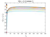
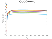
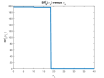
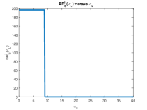
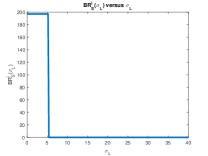
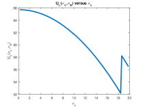
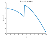
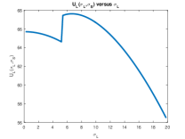
Figure 3: Row 1) User $i$ utility $U_{S}^{i}\left(\sigma_{L},\sigma_{S}^{-i},\sigma_{S}^{i}\right)$ versus $\sigma_{S}^{i}$ for various learner perturbation levels. Row 2) $BR_{S}^{i}\left(\sigma_{L}\right),$ based on the $\sigma_{S}^{i}$ which achieves the highest utility for each curve in Row 1. Row 3) Learner utility $U_{L}\left(\sigma_{L},BR_{S}^{i}\left(\sigma_{L}\right)\right),$ with $\sigma_{L}$ on the independent axis. From L to R, user perturbation cost $\bar{N}_{i}^{S}=10,20,30.$ As $\bar{N}_{i}^{S}$ increases, it becomes feasible for $L$ to perturb enough to discourage users from perturbing.

Because of the discontinuity in $U_{S}^{i}\left(\sigma_{L},\sigma_{S}^{-i},\sigma_{S}^{i}\right)$ introduced by the initial cost of perturbation, the best response function $\sigma_{S}^{i*}=BR_{S}^{i}\left(\sigma_{L}^{*}\right)$ is cumbersome to solve analytically. Therefore, we solve for the Stackelberg equilibrium numerically. Figure 3 displays the results, in which the three columns represent user perturbation cost $\bar{N}_{S}^{i}=10,20,30$ with other parameters held fixed.

Row 1 of the Fig. 3 depicts the optimization problem of the users. For $\sigma_{S}^{i}>0,$ the users pick $\sigma_{S}^{i}$ which optimally balances their individual privacy-accuracy preferences. This $\sigma_{S}^{i}$ could be large, because each user’s perturbation level affects his own accuracy only as one data point among many, whereas it directly affects improves privacy. At exactly $\sigma_{S}^{i}=0,$ however, the user’s utility jumps because he does not need to pay the perturbation cost. Row 2 illustrates this bang-bang behavior, which is summarized by Remark 8.

Remark 8.

At sufficiently-high $\sigma_{L}$ (the independent variable), the users’ privacy benefit becomes small enough that it is outweighed by the cost of perturbation, and $BR_{S}^{i}\left(\sigma_{L}\right)$ falls to $0.$ As $\bar{N}_{S}^{i}$ increases (from left to right in Fig. 3), the $\sigma_{L}$ to dissuade user perturbation decreases.

This raises the question of whether the benefit of dissuading user perturbation could be enough to justify the loss in accuracy and perturbation cost of adding $\sigma_{L}.$ Remark 9 states the numerical result shown in Row 3 of the figure.

Remark 9.

In Column 1 ($\bar{N}_{S}^{i}=10$), the $\sigma_{L}$ required to dissuade user perturbation is sufficiently high so that the benefits are outweighed by the loss in accuracy. In the other columns, the accuracy loss that $L$ experiences due to her own perturbation is overcome by the gain that she experiences when the users stop perturbing.

In Columns 2 and 3, the jumps in $U_{L}$ are high enough that they exceed the utility levels at $\sigma_{L}=0,$ and justify proactive perturbation. In general, the higher the user perturbation cost $\bar{N}_{S}^{i},$ the less $L$ needs to perturb to dissuade users from perturbing. The equilibrium in which $L$ perturbs proactively can be stated as follows.

1. Users prefer some privacy protection and are willing to invest in technology for obfuscation if necessary.

2. This obfuscation would be detrimental to $L.$

3. Instead, $L$ can perturb the data proactively.

4. $L$ need only match the users’ desires for privacy up to their perturbation costs $\bar{N}_{S}^{i}.$ Then the users are satisfied with $L$’s privacy protection and do not invest in obfuscation.

In some cases (i.e., Columns 2-4 of Fig. 3), $L$ improves his utility over cases in which the users perturb. Our findings do not guarantee this result in all cases, but provide a foundation for examining in which parameter regions $L$ can improve his utility by protecting privacy proactively.

VI Conclusion and Future Work

In this tracking-obfuscation interaction, the utility of each of the users are interrelated, since they all affect the accuracy of the output. Somewhat surprisingly, the optimal user perturbation levels as functions of the learner perturbation level are independent of one another. This leads to a self-interested behavior on the part of the users and a high accuracy loss on the part of the learner. In order to mitigate this problem, we have shown that a learner can sometimes dissuade users from data obfuscation by proactively perturbing collected information to some degree. Although she still must satisfy the users’ desired accuracy-privacy trade-off, she must only do so to within some constant: the flat cost of user perturbation. If user perturbation is sufficiently costly, privacy protection is incentive compatible for the learner. For future work, we anticipate studying an incomplete information version of the game, in which users’ privacy preferences are unknown, as well as a version of the game in which the number of players is a random variable. These steps will help to better understand and forecast the balance of power between user obfuscation and machine learning.

Appendix A Proofs of Accuracy Bound

Theorem 2 is proved using three lemmas. Lemma 10 bounds the difference between the perturbed and unperturbed classifiers.

Lemma 10.

(Bound on difference between classifiers) Assume that $\left|l^{\prime}\left(z\right)\right|\leq 1$ and $0\leq l^{\prime\prime}\left(z\right)\leq c.$ Then, for ERM with $L_{2}$-regularization, the magnitude of the difference between the unperturbed classifier $\mathbf{f^{\dagger}}$ and the input-perturbed classifier $\mathbf{f_{d}}$ is bounded in terms of $\left\|\mathbf{f_{d}}\right\|$ by the deterministic quantity:

$$\left\|\mathbf{f^{\dagger}}-\mathbf{f_{d}}\right\|^{2}\leq\frac{1+c^{2}\left\|\mathbf{f_{d}}\right\|^{2}}{n^{2}\Lambda^{2}}\underset{i}{\sum}\left\|\mathbf{v_{i}}+\mathbf{w_{i}}\right\|^{2}.$$ (12)

Essentially, the proof comes from comparing the first-order conditions for each of the classifiers. Note that when norms are not specified, we refer to the $L_{2}$-norm. Using this result, Lemma 11 bounds the difference in empirical loss.

Lemma 11.

(Bound in difference in empirical loss) For any realized database $D,$ the empirical loss is bounded by

$$J\left(\mathbf{f_{d}},D\right)-J\left(\mathbf{f^{\dagger}},D\right)\leq\left\|\mathbf{f_{d}}-\mathbf{f^{\dagger}}\right\|^{2}\left(1+c\right).$$ (13)

The proof of this lemma is based on work on empirical risk minimization in [7]. The next step is to bound the difference in expected loss using the difference in empirical loss. The result is given in Lemma 12.

Lemma 12.

(Bound in difference in expected loss) The difference in expected loss due to $\mathbf{f_{d}}$ and $\mathbf{f^{*}}$ satisfies, with probability $1-\delta,$

$$\hat{J}\left(\mathbf{f_{d}}\right)-\hat{J}\left(\mathbf{f}^{*}\right)\leq 2\left[J\left(\mathbf{f_{d}},D\right)-J\left(\mathbf{f^{\dagger}},D\right)\right]+O\left(\frac{\text{log}\left(1/\delta\right)}{\Lambda n}\right).$$ (14)

Define $\mathbf{u_{i}}\triangleq\mathbf{v_{i}}+\mathbf{w_{i}}.$ Using Lemma 10 and Lemma 11, with probability $1-\delta,$ $\hat{J}\left(\mathbf{f_{d}}\right)-\hat{J}\left(\mathbf{f}^{*}\right)\leq$

$$\frac{2+2c^{2}\left\|\mathbf{f_{d}}\right\|^{2}}{n^{2}\Lambda^{2}}\underset{i}{\sum}\left\|\mathbf{u_{i}}\right\|^{2}\left(1+c\right)+O\left(\frac{\text{log}\left(1/\delta\right)}{\Lambda n}\right),$$ (15)

Equation 14 is from Theorem 1 of [20], which bounds the difference between the expected loss of any classifier and the optimal classifier. Next, we bound $\left\|\mathbf{u_{i}}\right\|^{2}$ with some probability.

Lemma 13.

(Bound on error realization of random variables) Since $\mathbf{v_{i}}\sim\mathcal{V}_{i}$ and $\mathbf{w_{i}}\overset{\text{i.i.d.}}{\sim}\mathcal{W},$ $\mathbf{u_{i}}$ are draws from the distribution $\mathcal{V}_{i}+\mathcal{W}.$ From the cumulative distribution function of the $\chi^{2}$ variable, the square of their magnitude can be bounded with some probability by

$$\mathbb{P}\left\{\left\|\mathcal{\bar{V}}_{i}+\mathcal{\bar{W}}\right\|^{2}\leq\zeta\left(\sigma_{L}^{2}+\left(\sigma_{S}^{i}\right)^{2}\right)\right\}=\frac{\gamma\left(\frac{d}{2},\frac{\zeta}{2}\right)}{\Gamma\left(\frac{d}{2}\right)}.$$ (16)

The probability that the bound in Eq. 16 fails and that the bound in 15 fails is the product of the probability that each individually fails. Thus a conservative bound is $\hat{J}\left(\mathbf{f_{d}}\right)-\hat{J}\left(\mathbf{f}^{*}\right)\leq$

$$\frac{2+2c^{2}\left\|\mathbf{f_{d}}\right\|^{2}}{n^{2}\Lambda^{2}}\underset{i}{\sum}\zeta\left(\sigma_{L}^{2}+\left(\sigma_{S}^{i}\right)^{2}\right)\left(1+c\right)+O\left(\frac{\text{log}\left(1/\delta\right)}{\Lambda n}\right),$$ (17)

with probability at least $1-\delta\left(1-\gamma\left(\frac{d}{2},\frac{\zeta}{2}\right)/\Gamma\left(\frac{d}{2}\right)\right).$ This result leads to Theorem 2.

References

- [1] Continuous glucose monitoring for diabetes. WebMD, [Online]. Available: http://www.webmd.com/diabetes/guide/continuous-glucose-monitoring.
- [2] Privacy through visibility: disrupting nsa surveillance with algorithmically generated "scary" stories. University of Wisconsin-Milwaukee.
- [3] Internet of Things: Privacy and Security in a Connected World. Technical report, Federal Trade Commission, January 2015.
- [4] Tamer Baçar and Geert Jan Olsder. The Stackelberg Equilibrium Solution. In Dynamic Noncooperative Game Theory, volume 23 of Classics in Applied Mathematics. Academic Press, New York, 1999.
- [5] R. Baheti and H. Gill. Cyber-physical systems. The impact of control technology, 12:161–166, 2011.
- [6] Finn Brunton and Helen Nissenbaum. Obfuscation: A User’s Guide for Privacy and Protest. MIT Press, 2015.
- [7] Kamalika Chaudhuri, Claire Monteleoni, and Anand D Sarwate. Differentially private empirical risk minimization. The Journal of Machine Learning Research, 12:1069–1109, 2011.
- [8] Michela Chessa, Jens Grossklags, and Patrick Loiseau. A game-theoretic study on non-monetary incentives in data analytics projects with privacy implications. In Computer Security Foundations Symposium (CSF), 2015 IEEE 28th, pages 90–104. IEEE, 2015.
- [9] Michela Chessa, Jens Grossklags, and Patrick Loiseau. A short paper on the incentives to share private information for population estimates. In Financial Cryptography and Data Security, pages 427–436. Springer, 2015.
- [10] Cynthia Dwork. Differential privacy. In Automata, languages and programming, pages 1–12. Springer, 2006.
- [11] Cynthia Dwork and Moni Naor. On the difficulties of disclosure prevention in statistical databases or the case for differential privacy. Journal of Privacy and Confidentiality, 2(1):8, 2008.
- [12] Cynthia Dwork and Aaron Roth. The algorithmic foundations of differential privacy. Foundations and Trends in Theoretical Computer Science, 9(3-4):211–407, 2014.
- [13] Arpita Ghosh and Aaron Roth. Selling privacy at auction. Games and Economic Behavior, pages 334–346, 2015.
- [14] Daniel C. Howe and Helen Nissenbaum. TrackMeNot: Resisting surveillance in web search. Lessons from the Identity Trail: Anonymity, Privacy, and Identity in a Networked Society, 23:417–436, 2009.
- [15] Jonathan R. Mayer and John C. Mitchell. Third-party web tracking: Policy and technology. In Security and Privacy (SP), 2012 IEEE Symposium on, pages 413–427. IEEE, 2012.
- [16] Joseph Meyerowitz and Romit Roy Choudhury. Hiding stars with fireworks: location privacy through camouflage. In Proceedings of the 15th annual international conference on Mobile computing and networking, pages 345–356. ACM, 2009.
- [17] Robert S Parker, Francis J Doyle III, Nicholas Peppas, et al. A model-based algorithm for blood glucose control in type i diabetic patients. Biomedical Engineering, IEEE Transactions on, 46(2):148–157, 1999.
- [18] Scott R. Peppet. Regulating the Internet of Things: First Steps toward Managing Discrimination, Privacy, Security and Consent. Tex. L. Rev., 93:85, 2014.
- [19] Reza Shokri, George Theodorakopoulos, Carmela Troncoso, Jean-Pierre Hubaux, and Jean-Yves Le Boudec. Protecting location privacy: optimal strategy against localization attacks. In Proceedings of the 2012 ACM Conference on Computer and Communications Security, pages 617–627. ACM, 2012.
- [20] Karthik Sridharan, Shai Shalev-Shwartz, and Nathan Srebro. Fast rates for regularized objectives. In Advances in Neural Information Processing Systems, pages 1545–1552, 2009.
- [21] Melanie Swan. Sensor Mania! The Internet of Things, Wearable Computing, Objective Metrics, and the Quantified Self 2.0. Journal of Sensor and Actuator Networks, 1(3):217–253, November 2012.
- [22] Heinrich Von Stackelberg. Marktform und gleichgewicht. J. Springer, 1934.
- [23] David Xiao. Is privacy compatible with truthfulness? In Proceedings of the 4th conference on Innovations in Theoretical Computer Science, pages 67–86. ACM, 2013.