Analogues of glacial valley profiles in particle mechanics and in cosmology

An ordinary differential equation describing the transverse profiles of U-shaped glacial valleys, derived with a variational principle, has two formal analogies which we analyze. First, an analogy with point particle mechanics completes the description of the solutions. Second, an analogy with the Friedmann equation of relativistic cosmology shows that the analogue of a glacial valley profile is a universe with a future singularity but respecting the weak energy condition. The equation unveils also a Big Freeze singularity, which was not observed before for positive curvature index.

1 Introduction

It has long been acknowledged in glaciology since its inception [1, 2], and it is common knowledge also in elementary geography, that valleys carved by glaciers are U-shaped while valleys carved by the action of rivers are V-shaped. Here we focus on the former. The detailed and continued process of reshaping a valley by a glacier via erosion of the valley walls and bed over time is not simple and is best modelled with numerical techniques [3, 4, 5]. If one is interested only in the final result of the glacier action, simpler analytic approaches can be used. Given the scarcity of analytic models in the literature, theoretical approaches to this problem are valuable. A clever idea proposed by Hirano and Aniya in 1988 [6] consists of formulating a variational principle which extremizes the friction of the ice against the valley walls, subject to an appropriate constraint. Let the cross-sectional profile of a glacial valley be described by a function $y(x)$, where $x$ is a coordinate transverse to the glacier flow. Hirano and Aniya argued that friction (a functional of the cross-profile $y(x)$) should be minimum at the end of the erosion process, subject to the constraint that the contact length of the cross-profile of the ice is constant. This contact length between two endpoints $x_{1}$ and $x_{2}$ of the transverse profile is

$$s\left[y(x)\right]=\int_{x_{1}}^{x_{2}}ds=\int_{x_{1}}^{x_{2}}\sqrt{dx^{2}+dy^{2}}=\int_{x_{1}}^{x_{2}}\sqrt{1+(y^{\prime})^{2}}\,dx=\mbox{const.},$$ (1.1)

where a prime denotes differentiation with respect to $x$. The friction force is modelled by Coulomb’s law as $f=\mu N$, where $\mu$ is the friction coefficient and the normal force is $N=\rho ghA_{1}$. Here $\rho$ is the ice density, $g$ is the acceleration of gravity, $h$ is the ice thickness, and $A_{1}$ is the area of contact between the ice and the bed.

By considering a unit width of ice in the longitudinal direction of the glacier, the friction force due to an element of contact length $ds$ is $df=\mu Pds$. Further, $P=\eta(y_{s}-y)$, where $y_{s}$ denotes the ice surface and $\eta$ is a constant. Extremizing the friction

$$f\left[y(x)\right]=\mu\eta\int_{x_{1}}^{x_{2}}(y_{s}-y)\sqrt{1+(y^{\prime})^{2}}\,dx$$ (1.2)

subject to the constraint (1.1) leads to

$$\delta J=\mu\eta\,\delta\int_{x_{1}}^{x_{2}}\left(y_{s}-y+\lambda\right)\sqrt{1+(y^{\prime})^{2}}\,dx\equiv\delta\int_{x_{1}}^{x_{2}}L=0\,,$$ (1.3)

where $\lambda$ is a Lagrange multiplier and $L$ is the Lagrangian. The Euler-Lagrange equation

$$\frac{d}{dx}\left(\frac{\partial L}{\partial y^{\prime}}\right)-\frac{\partial L}{\partial y}=0$$ (1.4)

yields the ODE [6]

$$\frac{y_{s}-y+\lambda}{\sqrt{1+(y^{\prime})^{2}}}=c_{1}\,,$$ (1.5)

where $c_{1}$ is a constant. This equation is also obtained by solving the classic catenary problem of mechanics (e.g., [7], see Appendix A for further comments) and, therefore, it is not surprising that Hirano and Aniya obtained catenary solutions of eq. (1.5) [6].

Hirano and Aniya’s method and conclusions [6] have been criticized by Harbor [8] (see also the subsequent debate [9, 10, 11]). First, the assumptions in the model of [6] are inconsistent with other common assumptions in glaciology [8]. Second, friction should be maximized, not minimized [8] (although physically important, this change does not affect the first order variational principle, which only requires the friction integral to be extremized). In a reply to Harbor [9], Hirano and Aniya agree on this point but stand by the validity of application of the variational principle and of their previous result. Further critique by Morgan appeared fifteen years later [10]; he pointed out that there is no physical basis for the isoperimetric constraint (1.1), which should be replaced by the requirement that the area of the cross-section of the glacial valley be kept fixed instead. The rationale is that, by considering a unit width of ice in the direction of longitudinal flow, the ice volume is thus kept constant [8]. Indeed, it appears that Hirano and Aniya themselves had originally considered such a constraint, as they state in their reply to Morgan [11], although it did not appear in their original paper [9].

The new Lagrangian constraint of Morgan in the variational principle leads [10] to the ODE

$$\left(\frac{y^{\prime}}{y}\right)^{2}=\frac{1}{\left(\lambda y-C\right)^{2}}-\frac{1}{y^{2}}\,,$$ (1.6)

where $y(x)$ is now the ice thickness at transverse coordinate $x$, $\lambda$ is again a Lagrange multiplier, and $C$ is a constant, with $\lambda>1$ and $C>0$ required in order to have a smooth symmetric solution $y(x)$ on the interval $\left[-x_{0},x_{0}\right]$ with $y^{\prime}(0)=0$ [10]. Eq. (1.6) will be adopted in the rest of this work to describe transverse profiles of glacial valleys. An exact solution of eq. (1.6) was also provided in Ref. [10],

$$\left(\lambda^{2}-1\right)|x|=C\lambda\sqrt{1-w^{2}}+C\arccos w\,,$$ (1.7)

where

$$w=\left(\frac{\lambda^{2}-1}{C}\right)y-\lambda\,,$$ (1.8)

$$-\frac{1}{\lambda}\leq w\leq 1\,,\;\;\;\;\;\;\frac{C}{\lambda}\leq y\leq\frac{C}{\lambda-1}\,.$$ (1.9)

Another formal solution of eq. (1.6) for $\lambda^{2}<1$ is given in the recent reference [12]:

$$\pm\frac{\left(1-\lambda^{2}\right)^{3/2}}{|D|}\,x=\lambda\sqrt{w^{2}-1}+\ln\left|w+\sqrt{w^{2}-1}\right|+D\,,$$ (1.10)

where $D$ is an integration constant and $|w|>1$. For $C=0$ and $|\lambda|<1$ the solutions are linear.

The constraint of fixed cross-sectional area of the valley may perhaps seem questionable but no better one has been proposed in the literature thus far. The requirement of fixed cross-sectional area is also used in the numerical modelling of the erosion process leading to U-shaped valleys [4]. In any case, some constraint must be imposed because, if the friction integral is maximized without constraints, the first order variation

$$\delta\int_{x_{1}}^{x_{2}}\left(y_{s}-y\right)\sqrt{1+(y^{\prime})^{2}}\equiv\delta\int_{x_{1}}^{x_{2}}L_{0}=0\,,$$ (1.11)

where the Lagrangian is now

$$L_{0}\left(y(x),y^{\prime}(x)\right)=\left(y_{s}-y\right)\sqrt{1+(y^{\prime})^{2}}\,,$$ (1.12)

produces an equation which admits only solutions which are unphysical. In fact, since the Lagrangian (1.12) does not depend explicitly on $x$, the corresponding Hamiltonian

$${\cal H}_{0}=p_{y}y^{\prime}-L_{0}$$ (1.13)

is conserved, where

$$p_{y}=\frac{\partial L_{0}}{\partial(y^{\prime})}=\frac{\left(y_{s}-y\right)y^{\prime}}{\sqrt{1+(y^{\prime})^{2}}}$$ (1.14)

is the momentum canonically conjugated to $y$. The Euler-Lagrange equation (1.4) for $L_{0}$ has the first integral

$$\frac{\left(y_{s}-y\right)(y^{\prime})^{2}}{\sqrt{1+(y^{\prime})^{2}}}-\left(y_{s}-y\right)\sqrt{1+(y^{\prime})^{2}}=C\,,$$ (1.15)

where $C$ is a constant. Using the variable $\xi\equiv y_{s}-y>0$, eq. (1.15) is equivalent to

$$C\sqrt{1+(\xi^{\prime})^{2}}+\xi=0\,,$$ (1.16)

which requires that $C<0$, hence we set $C\equiv-C_{2}$, where $C_{2}>0$ is a constant with the dimensions of a length. Since $\xi\geq 0$, one obtains

$$\xi^{\prime}=\pm\sqrt{\frac{\xi^{2}}{C_{2}^{2}}-1}$$ (1.17)

which requires $\xi\geq C_{2}>0$. All the solutions $\xi(x)$ of eq. (1.17) are not bounded from above and are given by

$$y_{s}-y(x)=C_{2}^{2}\,\mbox{e}^{\mp\frac{(x-x_{0})}{C_{2}}}+\frac{\mbox{e}^{\pm\frac{(x-x_{0})}{C_{2}}}}{4}$$ (1.18)

(with $x_{0}$ another integration constant) and require $|x|\geq C_{2}$, which does not describe a valley geometry. Therefore, some Lagrangian constraint must be imposed when extremizing the friction integral $f[y(x)]$.

The fact that eq. (1.6) has an analogue in point particle mechanics seems to have been missed in the glaciology literature, while the fact that it has an analogue in the Friedmann equation of cosmology was noted in passing in the recent references [12, 13]. As we discuss in detail in Sec. 3 below, eq. (1.6) is a special case of Friedmann type equations which are of fundamental importance in cosmology. A mathematical peculiarity of this type of equations (and therefore also of eq. (1.6)) demonstrated in [13] is that the graphs of all the solutions (in our case, of the transverse valley profiles $y(x)$) are roulettes. A roulette is the locus of a point which lies on, or inside, a curve which rolls without slipping along a straight line.

Our goal is to explore the analogues of the ODE (1.6) in point particle mechanics and in cosmology, obtaining insight into the properties of this equation. In turn, we uncover a type of cosmological singularity which was studied recently [14] for spatially flat universes in the now abundant literature on cosmological singularities ([15, 16, 17, 18, 19, 20, 21, 22, 23] and references therein).

2 Particle mechanics analogues of glacial valley cross-profiles

We follow Ref. [10] and we assume that $C>0$ (but see the discussion below). The ODE (1.6) can be rewritten as

$$\frac{(y^{\prime})^{2}}{2}+V(y)=E\,,$$ (2.1)

where $(y^{\prime})^{2}/2$ can be regarded as the kinetic energy of a particle of unit mass in one-dimensional motion if $x$ and $y(x)$ are seen as the analogues of time and of the one-dimensional position, respectively, while

$$V(y)\equiv\frac{-y^{2}}{2\left(\lambda y-C\right)^{2}}$$ (2.2)

is an effective potential energy, and $E=-1/2$ is the total mechanical energy of the particle, which is fixed to this particular value. Newton’s second law of motion $y^{\prime\prime}=-dV/dy$ then rules the one-dimensional motion of the particle subject to the conservative force $-dV/dy$, and eq. (2.1) is a first integral corresponding to conservation of energy $E$ (with the fixed value $E=-1/2$). The solutions $y(x)$ corresponding to the possible motions of the particle are candidates for the description of cross-profiles of glacial valleys. As is well known from mechanics, a qualitative understanding of the motion can be obtained from the study of the potential $V(y)$ and of the intersections between its graph and the horizontal line $E=-1/2$ (which is called “Weierstrass approach” in various applications [29]-[31]).

It is $V(y)<0$  $\forall y\neq 0$,  $V(0)=0$,  $V(y)\rightarrow-1/(2\lambda^{2})$ as $y\rightarrow\pm\infty$, there is a vertical asymptote $y=C/\lambda>0$, and

$$V^{\prime}(y)=\frac{Cy}{\left(\lambda y-C\right)^{3}}\,,$$ (2.3)

therefore the function $V(y)$ is increasing for $y<0$ and for $y>C/\lambda$, decreasing for $0<y<C/\lambda$, and maximum at $y=0$ (see fig. 1).

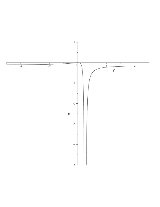
Figure 1: The potential $V(y)$ intersecting the horizontal line of constant energy $E=-1/2$ (the parameter values $\lambda=2$, $C=1$ are chosen for illustration).

We look for regions of bounded motions $y(x)>0$, corresponding to finite ice thickness. We restrict to the situation $C>0,\lambda>0$, for which the vertical asymptote $y=C/\lambda$ of $V(y)$ lies in the $y>0$ region. However, eq. (1.6) and the potential $V(y)$ are invariant under the exchange $\left(C,\lambda\right)\rightarrow\left(-C,-\lambda\right)$ and, formally, the situation $C<0,\lambda<0$ is the same as the one that we describe below.

2.1 The case $\lambda>1$

If $E=-\frac{1}{2}<-\frac{1}{2\lambda^{2}}$, corresponding to $|\lambda|>1$ (and we take $\lambda>1$ here), the horizontal line $E=-1/2$ describing the conserved energy of the particle associated with the glacial valley cross-profile lies below the horizontal asymptote of $V(y)$ (fig. 1). There are two regions corresponding to bounded motions $y(x)>0$ (we ignore the region $y<0$ because it is meaningless for the glacial valley problem). The first region is

$$0<y_{1}\leq y(x)<\frac{C}{\lambda}\,,$$ (2.4)

while the second region is

$$\frac{C}{\lambda}<y(x)\leq y_{2}\,,$$ (2.5)

where $y_{1,2}$ are turning points. The condition $\lambda>1$ is the condition for bounded solutions stated in Ref. [10], which now receives a graphical interpretation.

The particle cannot attain the position $y=C/\lambda$ where the potential becomes singular and is therefore confined to either the region (2.4) or the region (2.5).

The turning points $y_{1,2}$ are found analitically by setting equal to zero the kinetic energy $(y^{\prime})^{2}/2$ of the particle which leads, using eq. (1.6), to the quadratic algebric equation

$$\left(\lambda^{2}-1\right)y^{2}-2\lambda Cy+C^{2}=0\,.$$ (2.6)

The roots are

$$y_{1,2}=\frac{C}{\lambda\pm 1}\,.$$ (2.7)

The range

$$\frac{C}{\lambda}<y(x)\leq\frac{C}{\lambda-1}$$ (2.8)

reproduces the condition (1.9) reported in Ref. [10], while the range

$$\frac{C}{\lambda+1}\leq y(x)<\frac{C}{\lambda}$$ (2.9)

does not appear in the analysis of this reference, which is therefore augmented by the graphical mechanical analogy.

2.2 The case $\lambda=1$

If $E=-\frac{1}{2}=-\frac{1}{2\lambda^{2}}$, corresponding to $\lambda=1$, there is only unbounded motion in the region $y>C/\lambda$, but there is a region of bounded motion

$$y_{3}=\frac{C}{2}\leq y(x)<\frac{C}{\lambda}$$ (2.10)

which can make sense as the transverse profile of a glacial valley (see fig. 2).

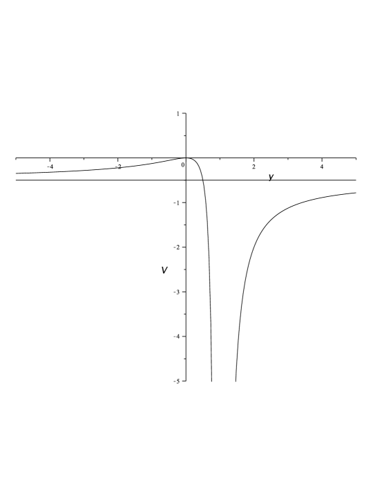
Figure 2: The potential $V(y)$ for $\lambda=1$. The horizontal line $E=-1/2$ intersects the graph of $V(y)$ only once for $y>0$ and there is a region, bounded by this intersection and by the vertical asymptote $y=C/\lambda$, which describes bounded motion. (The parameter value $C=1$ is used in this plot.)

As $\lambda\rightarrow 1^{+}$, one of the turning points (2.7) is pushed to infinity and effectively disappears, leaving a single turning point $y_{3}=C/2$.

2.3 The case $0<\lambda<1$

If $-\frac{1}{2\lambda^{2}}<E=-\frac{1}{2}$, corresponding to $\lambda<1$, the horizontal line of constant energy $E=-1/2$ lies above the horizontal asymptote of $V(y)$ and intersects the graph of $V(y)$ only once in the region $y>0$. There is a region of bounded motion

$$y_{4}\leq y(x)<\frac{C}{\lambda}\,.$$ (2.11)

The situation is qualitatively similar to the $\lambda=1$ case. The turning point $y_{4}=C/(1-\lambda)$ lies in the $y>0$ region, while the second turning point $y_{5}=-C/(1+\lambda)$ lies in the uninteresting region $y<0$. The analytic solution (1.10) of eq. (1.6) found in Ref. [12] belongs to this situation.

2.4 The case $\lambda<0$

We can now comment on the second condition $C>0$ appearing in Ref. [10] and assumed at the beginning of this section. Given the symmetry of eq. (1.6), the situation $C<0$ and $\lambda>0$ is equivalent to $C>0$ and $\lambda<0$, which we discuss here. In this case the vertical asymptote $y=C/\lambda$ of $V(y)$ lies in the $y<0$ region, and $V^{\prime}(y)$ is negative for $y<C/\lambda<0$ and for $y>0$, and is positive for $C/\lambda<y<0$. The graph of the potential energy $V(y)$ in this case is shown in fig. 3.

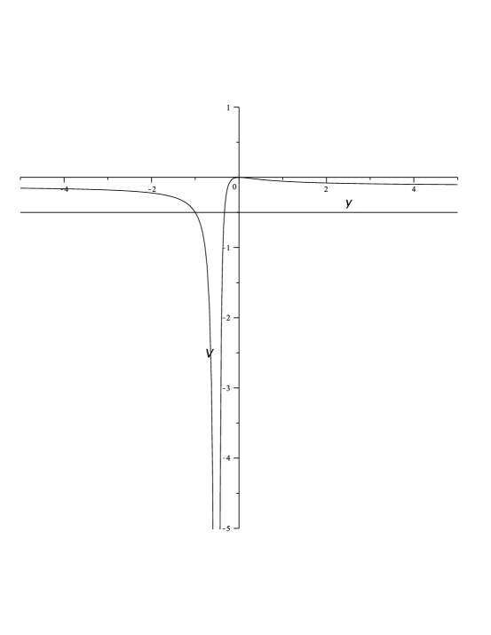
Figure 3: The potential $V(y)$ for negative $C$. In this case the motion is forbidden in the $y>0$ region if $E=-\frac{1}{2}\leq-\frac{1}{2\lambda^{2}}$. If $-1<\lambda<0$ the line $E=-1/2$ intersects the graph of $V(y)$ only at $y_{6}=C/(1+\lambda)$ in the $y>0$ region and there are no bounded motions. (The parameter values $\lambda=2$, $C=-1$ are chosen for illustration.)

If $E=-\frac{1}{2}>-\frac{1}{2\lambda^{2}}$ (corresponding to $-1<\lambda<0$), there is only one intersection $y_{6}=C/(1+\lambda)$ in the $y>0$ region and there are no bounded motions.

In the remaining case $C=0$, eq. (1.6) reduces to $(y^{\prime})^{2}=-1+1/\lambda^{2}$, which has linear solutions corresponding to V-shaped valleys irrelevant as glacial valley cross-profiles (except perhaps as initial conditions, see, e.g., [4]). This is the reason why we assumed that $C>0$ and we will restrict to this range of the parameter $C$ in the rest of this work.

2.5 Analogue of the no-constraint equation

Finally, we comment on the incorrect equation (1.17) which would be obtained by extremizing friction without any Lagrangian constraint. Using the mechanical analogy, eq. (1.17) can be rewritten as the energy integral of motion

$$\frac{(\xi^{\prime})^{2}}{2}+U(\xi)=E\,,$$ (2.12)

where $E=-1/2$ and the potential energy

$$U(\xi)=-\frac{\xi^{2}}{2C_{2}^{2}}$$ (2.13)

corresponds to an inverted harmonic oscillator. Therefore, all trajectories (except for the unstable equilibrium position $\xi\equiv 0$, which is meaningless in the original valley glacier problem) are unbounded and unphysical as glacier cross-profiles.

3 The universe in a glacial valley

Relativistic cosmology (e.g., [15, 32, 33]) is obtained by assuming that the 4-dimensional spacetime of general relativity is spatially homogeneous and isotropic about every point of 3-space. This assumption is motivated by the fact that, on scales of hundreds of megaparsecs, the matter distribution and the cosmic microwave background are spatially homogenous and isotropic [33, 15, 32]. The cosmic microwave background, in particular, is highly isotropic apart from tiny temperature fluctuations $\delta T/T\sim 10^{-5}$ imprinted early on by large-scale structures, which play a major role in our investigations of the early universe [34]. These assumptions lead uniquely to the Friedmann-Lemaître-Robertson-Walker (FLRW) line element of spacetime [15, 32, 33]

$$ds^{2}=-dt^{2}+a^{2}(t)\left[\frac{dr^{2}}{1-kr^{2}}+r^{2}\left(d\theta^{2}+\sin^{2}\theta\,d\varphi^{2}\right)\right]$$ (3.1)

in polar coordinates $\left(t,r,\theta,\varphi\right)$, where $t$ is the time of the observers who see the cosmic microwave background homogeneous and isotropic around them apart from the tiny fluctuations (comoving observers). The positive function $a(t)$ (scale factor) describes how any two points of space (for example two typical comoving galaxies) separate in time as the universe expands (which is described by an increasing function $a(t)$). $k$ is the curvature index normalized to the possible values $k=-1$ (open universe), $k=0$ (critically open or spatially flat universe), or $k=+1$ (closed universe) [15, 32, 33]. Following the literature on cosmology, we use units in which the speed of light $c$ is unity. It is usually assumed in cosmological investigations that the material content of the universe is in the form of a perfect fluid of energy density $\rho$ and pressure $P$, as measured by the comoving observers. Once an equation of state for the fluid linking $P$ and $\rho$ is specified, one can solve the Einstein equations for the spacetime metric $g_{ab}$ giving the line element through $ds^{2}=g_{ab}dx^{a}dx^{b}$ (we use the Einstein summation convention over repeated indices). Because, due to spatial homogeneity and isotropy, the line element must assume the FLRW form (3.1), the only degree of freedom is the scale factor $a(t)$ and the Einstein field equations, which are usually PDEs, reduce to the Einstein-Friedmann ODEs for $a(t)$ [15, 32, 33]

$$H^{2} \equiv \frac{\dot{a}^{2}}{a^{2}}=\frac{8\pi G}{3}\,\rho-\frac{k}{a^{2}}\,,$$ (3.2)

$$\frac{\ddot{a}}{a} = -\frac{4\pi G}{3}\left(\rho+3P\right)\,,$$ (3.3)

where an overdot denotes differentiation with respect to the comoving time $t$ and $H(t)\equiv\dot{a}/a$ is the Hubble function. $G$ is Newton’s constant expressing the strength of the coupling between gravity and matter. Eq. (3.2) is often referred to as the Friedmann equation.

In general relativity, the pressure $P$ of the cosmic fluid gravitates together with the energy density $\rho$ and the combination $\rho+3P$ in eq. (3.3) determines whether the universe accelerates ($\ddot{a}>0$) or decelerates ($\ddot{a}<0$) its expansion.

A third convenient (but not independent) equation can be derived from the previous two:

$$\dot{\rho}+3H\left(P+\rho\right)=0$$ (3.4)

and it expresses covariant conservation of the energy-momentum tensor of the cosmic fluid [15, 32, 33].

The Friedmann equation (3.2) is the analogue in cosmology of eq. (1.6) describing the ice thickness in glacial valley transverse profiles. The analogy was noted recently, but not pursued, in Ref. [13]. Although one can attempt an analogy with universes corresponding to different values of the curvature index $k$ in eq. (3.1), the most straightforward identification between eqs. (1.6) and eq. (3.2) is achieved by setting $k=1$, which corresponds to a closed universe analogue of the glacial valley profile. The cosmological analogue of eq. (1.6)

$$\frac{\dot{a}^{2}}{a^{2}}=\frac{1}{\left(\lambda a-C\right)^{2}}-\frac{1}{a^{2}}$$ (3.5)

can be rewritten as

$$\frac{\dot{a}^{2}}{a^{2}}=\frac{8\pi G}{3}\,\frac{\rho_{0}}{\left(a-a_{0}\right)^{2}}-\frac{1}{a^{2}}\,,$$ (3.6)

where

$$\rho_{0}=\frac{3}{8\pi G\lambda^{2}}\,,\;\;\;\;\;a_{0}=\frac{C}{\lambda}$$ (3.7)

are positive constants. Eq. (3.2) gives immediately the energy density of the analogue cosmic fluid as

$$\rho(t)=\frac{\rho_{0}}{\left(a-a_{0}\right)^{2}}\,.$$ (3.8)

Two properties of the function $\rho(t)$ are relevant. First, the energy density is always positive, which is expected of “reasonable” forms of matter but is not guaranteed in any formal analogy of ODEs with the equations of FLRW cosmology (indeed, the identification of eq. (1.6) with the cosmological equation (3.2) with curvature index $k\leq 0$ gives rise to negative effective energy densities $\rho$ when $a\rightarrow 0$, an unphysical property which would detract from the analogy). Second, the density diverges if $a\rightarrow a_{0}$: this divergence corresponds to a true spacetime singularity (as opposed to a coordinate singularity) and is discussed below.

“Reasonable” matter in general relativity is supposed to satisfy certain energy conditions which, essentially, prohibit negative energy densities and energy flows faster than the speed of light [15, 32, 33]. When applied to a perfect fluid with energy density $\rho$ and pressure $P$, the two energy conditions which are most often encountered in the literature (and that are relevant below) are the weak energy condition, which amounts to $\rho\geq 0$ and $\rho+P\geq 0$, and the strong energy condition $\rho+P\geq 0$ and $\rho+3P\geq 0$ [32, 15, 33].

Let us proceed by deducing the effective pressure $P$ of the analogue cosmic fluid by imposing eq. (3.4), which yields

$$P=\frac{2\rho_{0}a}{3\left(a-a_{0}\right)^{3}}-\frac{\rho_{0}}{\left(a-a_{0}\right)^{2}}$$ (3.9)

and can be rewritten as

$$P=-\frac{\rho}{3}\pm\frac{2a_{0}}{3\sqrt{\rho_{0}}}\,\rho^{3/2}\,,$$ (3.10)

where the upper sign applies when $a>a_{0}$ and the lower sign when $a<a_{0}$. Using eq. (3.9), it is seen that the condition $\rho+P>0$ corresponds to $a>a_{0}$ and, vice-versa, violation of this condition corresponds to $a<a_{0}$. Equations of state of the cosmic fluid corresponding to the lower sign in eq. (3.10) and violating the weak energy condition have been discussed in Ref. [18]. Equations of state of the cosmic fluid of the form $P=\sum_{k=1}^{m}c_{k}\rho_{(k)}^{k}$ have been studied in [12, 13]. Quadratic equations of state, in particular, have been the subject of further attention [35, 36, 37, 38, 39, 40] but pressures depending on fractional powers of the density have not been studied. As shown below, they give rise to a peculiar type of singularities. While traditional cosmology and relativity textbooks report only linear barotropic equations of state $P=P_{0}+A\rho$, following the discovery of the acceleration of the universe in 1998, the literature abounds with exotic non-linear equations of state for the dark energy fluid postulated in order to explain this acceleration.

Let us consider now the acceleration equation (3.3) which, using eq. (3.9), reduces to

$$\frac{\ddot{a}}{a}=-\frac{a_{0}}{\lambda^{2}\left(a-a_{0}\right)^{3}}\,.$$ (3.11)

Clearly, the universe is accelerated if $a<a_{0}$ (corresponding to $\rho+3P<0$) and decelerated if $a>a_{0}$ (corresponding to $\rho+3P>0$).

The value $a_{0}$ of the scale factor corresponds to a spacetime singularity, which is seen as follows. The Einstein equations

$$R_{ab}-\frac{1}{2}\,g_{ab}R=8\pi GT_{ab}$$ (3.12)

(where $R_{ab}$ is the Ricci tensor and $R\equiv g^{ab}R_{ab}$ is its trace, while $g^{ab}$ is the inverse of the metric tensor $g_{ab}$) can be traced to give

$$R\equiv{R^{a}}_{a}=-8\pi GT\,,$$ (3.13)

where $T\equiv{T^{a}}_{a}$ is the trace of the perfect fluid energy momentum tensor [15, 32, 33]

$$T_{ab}=\left(P+\rho\right)u_{a}u_{b}+Pg_{ab}$$ (3.14)

and $u^{a}$ is the 4-velocity of the cosmic fluid (equivalently, the 4-velocity of comoving observers). One obtains the Ricci scalar

$$R=8\pi G\left(\rho-3P\right)=\frac{16\pi G\rho_{0}}{\left(a-a_{0}\right)^{3}}\left(a-2a_{0}\right)\,,$$ (3.15)

which diverges in the limit $a\rightarrow a_{0}$, signalling a spacetime singularity. However, it is not yet clear whether the value $a_{0}$ of the scale factor, which corresponds to a spacetime singularity and diverging density and pressure, can actually be approached during the dynamics of the scale factor $a(t)$. In order to answer this question note that eq. (3.2), which is of only first order, constitutes a dynamical constraint since it must be $H^{2}\geq 0$, which can be written as

$$a^{2}\geq\lambda^{2}\left(a-a_{0}\right)^{2}$$ (3.16)

using $k=+1$. The condition (3.16) excludes the orbits of the solutions of the dynamical system (3.2), (3.3) from a certain volume of the $\left(a,\dot{a}\right)$ phase space. This constraint plays the role that the first integral expressing conservation of energy plays in point particle mechanics by confining the orbits of the solutions to an energy surface $E=$ const. in phase space.

If $a>a_{0}$, the dynamical constraint (3.16) can be written as $a\leq\lambda a_{0}/(\lambda-1)$. The coefficient of $a_{0}$ is $\frac{\lambda}{\lambda-1}=1+\frac{1}{\lambda-1}>1$ and therefore, in this regime we have

$$a_{0}<a<\frac{\lambda a_{0}}{\lambda-1}\,:$$ (3.17)

the scale factor $a(t)$ cannot grow arbitrarily large but is bounded from above. However, it can get arbitrarily close to the value $a_{0}$ corresponding to the singularity.

If instead $a<a_{0}$, then the constraint (3.16) becomes $a\geq\lambda a_{0}/(\lambda+1)$, hence in this regime one has

$$0<\frac{\lambda a_{0}}{\lambda+1}\leq a<a_{0}\,.$$ (3.18)

In both cases the scale factor is bounded from below by a positive constant (hence one cannot have a Big Bang- or Big Crunch-type singularity, which would correspond to $a\rightarrow 0$ [15, 32, 33]) but it can reach the singularity $a_{0}$. The fact that one cannot have $y=0$ in the original equation (1.6) because it implies an imaginary $y^{\prime}$ was noted as “a curious feature” in Ref. [10]. It corresponds to the fact that $y=0$ (equivalently, $a=0$) lies in the region of the phase space forbidden by the constraint (3.16).

The boundary values $a=\lambda a_{0}/(\lambda\mp 1)$ are formal solutions of eq. (3.5) obtained by setting $a=$ constant, but they do not satisfy eq. (3.3) (they would be meaningless anyway as analogues of glacial valley profiles).

Consider again the acceleration equation (3.3): if $a>a_{0}$, then $\ddot{a}<0$ and the curve representing the scale factor has concavity facing downwards, describing a decelerated universe. Since this curve is continuous, it must always decrease and eventually cross the horizontal line $a=a_{0}$ (see fig. 4).

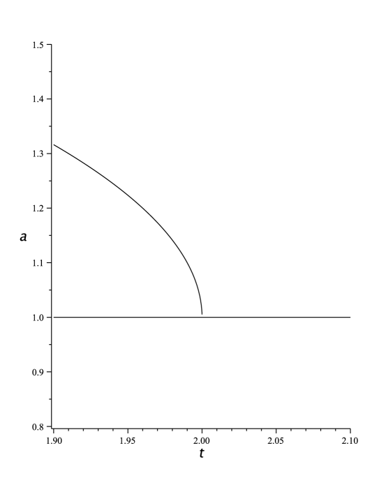
Figure 4: The behavior of the scale factor $a(t)$ near the singularity $a_{0}$ when $a>a_{0}$ (for the parameter values $a_{0}=1$, $t_{0}=2$). The concavity faces downward and the universe is decelerated.

Using eq. (3.7), eq. (3.5) is written as

$$\dot{a}^{2}=\frac{a^{2}}{\lambda^{2}\left(a-a_{0}\right)^{2}}-1\approx\frac{a_{0}^{2}}{\lambda^{2}\left(a-a_{0}\right)^{2}}$$ (3.19)

as $a\rightarrow a_{0}$. This asymptotic equation is easily integrated, giving

$$a(t)\simeq a_{0}\pm\sqrt{\frac{2a_{0}}{\lambda}|t-t_{0}|}\,,$$ (3.20)

where the integration constant $t_{0}$ has the meaning of time at which the singularity occurs and the positive sign must be chosen in front of the square root because it is $a>a_{0}$. This situation constitutes a physically meaningful analogue of glacial valleys because $y$ is the thickness of the ice (maximum at $x=0$ and minimum at the valley boundaries) and it is interesting in cosmology because it provides an example of a finite time singularity even when $\rho>0$ and $\rho+P>0$, i.e., without violating the weak energy condition. This kind of situation was discussed in Ref. [18].

Vice-versa, if $a<a_{0}$, then it is $\ddot{a}>0$ and $a(t)$ always increases, eventually crossing the horizontal line $a=a_{0}$ (fig. 5).

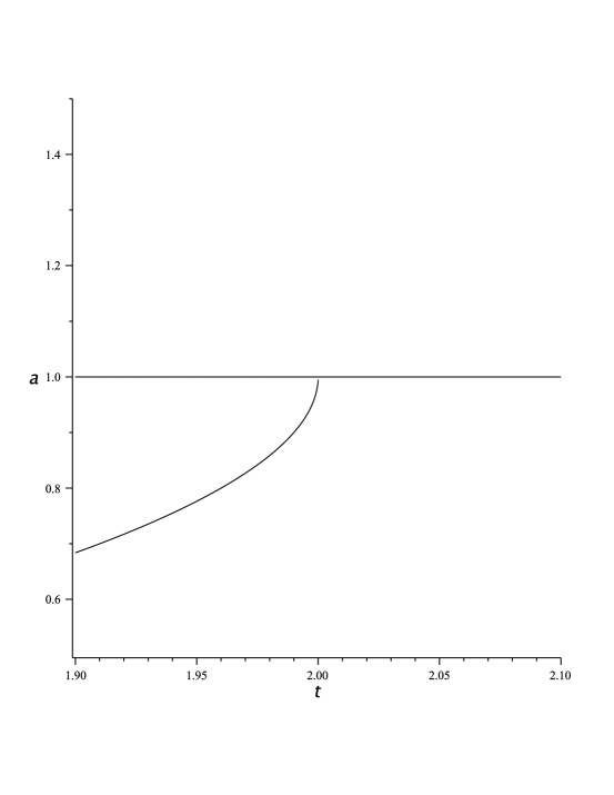
Figure 5: The behavior of the scale factor $a(t)$ near the singularity $a_{0}$ when $a<a_{0}$ (for the parameter values $a_{0}=1$, $t_{0}=2$). The concavity faces upward and the universe is accelerated.

The asymptotic equation (3.19) is now integrated to

$$a(t)\simeq a_{0}-\sqrt{\frac{2a_{0}}{\lambda}|t-t_{0}|}$$ (3.21)

choosing the negative sign in front of the square root because it is now $a<a_{0}$. This situation is not a meaningful analogue of a glacial valley cross-profile. The slope of this function becomes infinite where $a(t)$ crosses the value $a_{0}$, and this boundary corresponds to the spacetime singularity in the cosmological analogue. In this case the universe has a minimum size $a_{min}=\lambda a_{0}/(\lambda+1)$ and it bounces upon reaching it. It is well known in cosmology that such a bounce occurs when the weak energy condition $\rho+P<0$ is violated, which is exactly what is happening here since

$$\rho+P=\frac{2\rho_{0}a}{3\left(a-a_{0}\right)^{3}}<0\,.$$ (3.22)

The violation of the weak energy condition signals that the cosmic fluid is of a very exotic form referred to as phantom energy, which causes the universe to accelerate in such a way that the Hubble function increases according to

$$\dot{H}=-4\pi G\left(\rho+P\right)+\frac{k}{2a^{2}}>0$$ (3.23)

if $k\geq 0$. (This equation can be obtained by differentiating eq. (3.2) and substituting eqs. (3.2) and (3.3) into the result.) This is a very unusual situation (called superacceleration) and causes the universe to expand super-exponentially and reach a singularity at a finite time. In the standard cosmological literature the scale factor of a phantom-dominated universe diverges at a finite time in the future at a Big Rip singularity [17], but here the situation is different since the scale factor stays finite while the Hubble function $H$, energy density $\rho$, pressure $P$, and Ricci scalar $R$ all diverge as $a\rightarrow a_{0}$. This situation corresponds instead to a type of singularity studied recently in spatially flat (i.e., $k=0$) universes and called Big Freeze singularity [14] or Type III singularity in the classification of [24]. A Big Freeze singularity appears also in cosmology in the context of Palatini $f(R)$ gravity [25, 26, 27, 28]. This is a class of theories of gravity alternative to general relativity and attempting to explain the present acceleration of the universe without dark energy. A Big Freeze singularity was not reported before for positively curved (i.e., $k>0$) universes. The reason why here the situation is essentially the same as for spatially flat universes is that, as $a\rightarrow a_{0}$ in eq. (3.6), the divergent term proportional to $\left(a-a_{0}\right)^{-2}$ in the energy density dominates over the curvature term $-1/a^{2}$, which is finite and becomes irrelevant. Finite time singularities, including Big Rip [17] and sudden future singularitities [16, 18], have been the subject of a significant amount of work in cosmology (see [41, 42, 43, 19, 20, 21, 22, 14, 24, 23] and the extensive literature originating from these references).

Finally, although it is not interesting for the original glacial valley problem, the cosmic analogue of eq. (1.6) for $C=0$ (noted also in [13]) corresponds to $a_{0}=0$ and

$$H^{2}=\frac{1}{a^{2}}\left(\frac{1-\lambda^{2}}{\lambda^{2}}\right)$$ (3.24)

and requires $|\lambda|\leq 1$. Then $\dot{a}=$ const. and the solutions are linear in time and include a static universe with $a=$ const. as a special case.

4 Discussion

In glacial morphology studies, researchers content themselves with fitting data of glacial valley cross-profiles with parabolas $y(x)=ax^{2}+bx+c$ (following an early practice initiated by Svennsson [44] which is not free of critique, see e.g., [45]). Other fitting curves used include power-law profiles $y(x)=ax^{b}$, possibly with different powers $b$ for each half-profile going from the bottom at $x=0$ to each valley side.

There is a deep disconnect between theory and practice here. Since a parabola is just the second order Taylor expansion of any sufficiently regular function with a minimum, which could solve any ODE, data fitting with parabolas is of no help when one attempts to test models and to discriminate between various theoretical approaches to the problem of the cross-sectional profiles of glacial valleys, which predict different ODEs for the profile $y(x)$. In this sense fitting parabolas, or even power-laws, is deeply unsatisfactory from the theoretical point of view. Determining the best-fit parameters of a parabola for a glacial valley, or an ensemble of valleys, does not contribute to understanding the mechanism that generated them.

Here we focused on the variational principle approach to the problem of glacial valley erosion, in the form given by Morgan [10] which imposes that the cross-sectional area of the valley is fixed as a Lagrangian constraint. This condition is also used in modern numerical modelling of the detailed glacial erosion process (e.g., [4]). The resulting eq. (1.6) for the ice thickness $y(x)$ has an analogue in point particle mechanics and one in cosmology, both of which contribute to a better understanding of the character of this ODE, of its solutions, and of the conditions (on the parameters $\lambda$ and $C$) for their physical viability. We developed these analogies in detail. The previous analysis [10] is augmented by the graphical analysis of the effective potential $V(y)$ in the mechanical analogy. In turn, the problem of glacial valley profiles provides an interesting example of a finite time singularity in cosmology without violating the weak energy condition. The finite time singularity is caused by the peculiar effective equation of state (3.10) which falls into the broader category $P=w\rho-\alpha\rho^{m}$ (with $w,\alpha$, and $m$ constants) which has been the subject of wide interest in cosmology but restricted to integral values of the exponent $m$ [18, 41, 42, 43, 19].

The present work also highlights two open problems in glaciology. First, the friction of glacier ice against the valley walls and bed is unlikely to be described purely by Coulomb’s law, but it should include viscous friction which depends on the velocity (a friction model quadratic in the velocity is used, for example, in the numerical work [4]). Second, the numerical analyses of the formation of glacial valleys ignore the variational approach (but not its Lagrangian constraint) and should be compared with it. These issues will be revisited in future work.

Appendices

A The catenary problem

The classic catenary problem (e.g., [7]) gives rise to the same ODE (1.5) obtained by Hirano and Aniya in [6]. Consider a heavy string hanging in a vertical $\left(x,y\right)$ plane and described by the profile $y(x)$. The linear density is $\mu=dm/ds$, where $ds=\sqrt{dx^{2}+dy^{2}}=\sqrt{1+(y^{\prime})^{2}}\,dx$ is the line element along the string. The gravitational potential energy of an element of string of length $ds$ located at horizontal position $x$ is $dE_{g}=\mu gy(x)ds$. The total gravitational potential energy of a string suspended by two points of horizontal coordinates $x_{1}$ and $x_{2}$ is the functional of the curve $y(x)$

$$E_{g}\left[y(x)\right]=\mu g\int_{x_{1}}^{x_{2}}dx\,y\sqrt{1+(y^{\prime})^{2}}\equiv\int_{x_{1}}^{x_{2}}L\,dx\,.$$ (A.1)

The Lagrangian $L\left(y(x),y^{\prime}(x)\right)$ does not depend explicitly on the coordinate $x$ and, therefore, the corresponding Hamiltonian is conserved:

$${\cal H}=\frac{\partial L}{\partial(y^{\prime})}\,y^{\prime}-L=c_{1}\,,$$ (A.2)

where $c_{1}$ is a constant. This equation simplifies to

$$\frac{-y}{\sqrt{1+(y^{\prime})^{2}}}=c_{1}\,,$$ (A.3)

which has catenaries as solutions [7]. With the change of variable $y\rightarrow\bar{y}\equiv y-y_{s}-\lambda$, eq. (1.5) reduces to the same form as eq. (A.3) and it is not surprising that Hirano and Aniya find catenary solutions [6].

Although not necessary, the variational principle is sometimes imposed subject to the constraint that the string length between $x_{1}$ and $x_{2}$ is fixed, which changes the variational integral to

$$J\left[y(x)\right]=\int_{x_{1}}^{x_{2}}dx\,\left(y+\lambda\right)\sqrt{1+(y^{\prime})^{2}}\,,$$ (A.4)

where $\lambda$ is a Lagrange multiplier.

The cosmological analogue of eq. (A.3) corresponds to a well known situation in cosmic physics. This equation is recast as

$$\left(\frac{y^{\prime}}{y}\right)^{2}=\frac{1}{C_{1}^{2}}-\frac{1}{y^{2}}\,,$$ (A.5)

the analogue of which for the scale factor $a(t)$ reads

$$\frac{\dot{a}^{2}}{a^{2}}=\frac{\Lambda}{3}-\frac{1}{a^{2}}\,,$$ (A.6)

where $\Lambda=3/C_{1}^{2}>0$ is the cosmological constant. The cosmological constant corresponds to the modification of the Einstein equations [15, 32, 33]

$$R_{ab}-\frac{1}{2}\,g_{ab}R+\Lambda g_{ab}=8\pi GT_{ab}\,,$$ (A.7)

but it can be treated as a special case of a perfect fluid by taking the $\Lambda$-term to the right hand side and treating it as an effective stress-energy tensor $T_{ab}=-\Lambda g_{ab}/(8\pi G)$, which has the perfect fluid form (3.14) with energy density and pressure [15, 32, 33]

$$\rho_{\Lambda}=\frac{\Lambda}{8\pi G}=-P_{\Lambda}\,.$$ (A.8)

A positive cosmological constant violates the strong energy condition $\rho+3P\geq 0$ and essentially corresponds to repulsive gravity [32, 33, 46]. The de Sitter expansion $a(t)=\mbox{const.}\,\mbox{e}^{Ht}$ with constant Hubble function $H$ gives a solution of the Einstein-Friedmann equations with $\Lambda$ as the only material source if $k=0$ and is an attractor for the $k=0$ spaces filled with other matter sources in addition to $\Lambda$, and also for the $k\neq 0$ cases. The importance of the de Sitter space in cosmology can hardly be overemphasized, since this solution is an attractor for the regime of slow-roll inflation in the early universe [47, 33] and in the late universe [46].

References

- [1] J.F. Campbell, Frost and Fire (J.B. Lippincott, Philadelphia, 1865).
- [2] W.J. McGee, “Glacial Canons”, J. Geology 2, 350-364 (1894).
- [3] J.M. Harbor, “Development of glacial-valley cross sections under conditions of spatially variable resistance to erosion”, Geomorphology 14, 99-107 (1995).
- [4] H. Seddik, R. Greve, and S. Sugiyama, “Numerical simulation of the evolution of glacial valley cross sections”, preprint arXiv:0901.1177 (2009).
- [5] S.H. Yang and Y.L. Shi, “Three-dimensional numerical simulation of glacial trough forming process”, Science China (Earth Sciences) 58, 1656-1668 (2015).
- [6] M. Hirano and M. Aniya, “A rational explanation of cross-profile morphology for glacial valleys and of glacial valley development”, Earth Surf. Process. Landforms 13, 707-716 (1988).
- [7] H. Goldstein, Classical Mechanics (Addison-Wesley, Reading, MA, 1980).
- [8] J. Harbor, “A discussion of Hirano and Aniya’s (1988, 1989) explanation of glacial-valley cross profile development”, Earth Surf. Process. Landforms 15, 369-377 (1990).
- [9] M. Hirano and M. Aniya, “A reply to ‘A discussion of Hirano and Aniya’s (1988, 1989) explanation of glacial-valley cross profile development’ by Jonathan M. Harbor”, Earth Surf. Process. Landforms 15, 379-381 (1990).
- [10] F. Morgan, “A note on cross-profile morphology for glacial valleys”, Earth Surf. Process. Landforms 30, 513-514 (2005).
- [11] M. Hirano and M. Aniya, “Response to Morgan’s comment”, Earth Surf. Process. Landforms 30, 515 (2005).
- [12] S. Chen, G.W. Gibbons, and Y. Yang, “Explicit integration of Friedmann’s equation with nonlinear equations of state”, J. Cosmol. Astropart. Phys. 05, 020 (2015).
- [13] S. Chen, G.W. Gibbons, and Y. Yang, “Friedmann-Lemaitre cosmologies via roulettes and other analytic methods”, J. Cosmol. Astropart. Phys. 10, 056 (2015).
- [14] M. Bouhmadi-Lopez, P.F. Gonzalez-Diaz, and P. Martin-Moruno, “Worse than a big rip?”, Phys. Lett. B 659, 1-5 (2008).
- [15] R.M. Wald, General Relativity (Chicago University Press, Chicago, 1984).
- [16] J.D. Barrow, G. Galloway, and F.J.T. Tipler, “The closed-universe recollapse conjecture”, Mon. Not. R. Astron. Soc. 223, 835-844 (1986).
- [17] R.R. Caldwell, “A phantom menace? Cosmological consequences of a dark energy component with super-negative equation of state”, Phys. Lett. B 545, 23-29 (2002).
- [18] J.D. Barrow, “Sudden future singularities”, Class. Quantum Grav. 21, L79-L82 (2004).
- [19] V. Sahni and Y. Shtanov, “Unusual cosmological singularities in brane world models”, Class. Quantum Grav. 19, L101-L107 (2002).
- [20] M.P. Dabrowski, T. Denkiewicz, M.A. Hendry, “How far is it to a sudden future singularity of pressure?”, Phys. Rev. D 75, 123524 (2007).
- [21] M.P. Dabrowski and T. Denkiewicz, “Barotropic index -singularities in cosmology”, Phys. Rev. D 79, 063521 (2009).
- [22] L. Fernandez-Jambrina, “Hidden past of dark energy cosmological models”, Phys. Lett. B 656, 9-14 (2007).
- [23] J. Beltrán Jiménez, D. Rubiera-Garcia, D. Sáez-Gómez, and V. Salzano, “Q-singularities”, preprint arXiv:1607.06389.
- [24] K. Bamba, S. Capozziello, S. Nojiri, and S.D. Odintsov, “Dark energy cosmology: the equivalent description via different theoretical models and cosmography tests”, Astrophys. Space Sci. 342, 155-228 (2012).
- [25] A. Borowiec, M. Kamionka, A. Kurek, and M. Szydlowski, “Cosmic acceleration from modified gravity with Palatini formalism”, J. Cosmol. Astropart. Phys. 1202, 027 (2012).
- [26] A. Borowiec, A. Stachowski, M. Szydlowski, and A. Wojnar, “‘Inflationary cosmology with Chaplygin gas in Palatini formalism”, J. Cosmol. Astropart. Phys. 1601, 040 (2016).
- [27] A. Stachowski, M. Szydlowski, and A. Borowiec, “Starobinsky cosmological model in Palatini formalism”, arXiv:1608.03196.
- [28] M. Szydlowski, A. Stachowski, A. Borowiec, and A. Wojnar, “Do sewn singularities falsify the Palatini cosmology?”, arXiv:1512.04580.
- [29] M. Destrade, G. Gaeta, and G. Saccomandi, “Weierstrass criterion and compact solitary waves”, Phys. Rev. E 75, 047601 (2007).
- [30] I. Bochicchio and E. Laserra, “On the mechanical analogy between the relativistic evolution of a spherical dust universe and the classical motion of falling bodies”, J. Interdiscip. Math. 10, 747-755 (2007).
- [31] I. Bochicchio, S. Capozziello, and E. Laserra, “The Weierstrass criterion and the Lemaître-Tolman-Bondi models with cosmological constant”, Int. J. Geom. Meth. Mod. Phys. 8, 1653-1666 (2011).
- [32] S.M. Carroll, Spacetime and Geometry: An Introduction to General Relativity (Addison Wesley, San Francisco, 2004).
- [33] A. Liddle, An Introduction to Modern Cosmology (Wiley, Chichester, 2003).
- [34] R. Durrer, The Cosmic Microwave Background (Cambridge University Press, Cambridge, 2008).
- [35] K.N. Ananda and M. Bruni, “Cosmodynamics and dark energy with non-linear equation of state: a quadratic model”, Phys. Rev. D 74, 023523 (2006).
- [36] K.N. Ananda and M. Bruni, “Cosmodynamics and dark energy with a quadratic EoS: anisotropic models, large-scale perturbations and cosmological singularities”, Phys. Rev. D 74, 023524 (2006).
- [37] S. Silva e Costa, “An entirely analytical cosmological model”, Mod. Phys. Lett. A 24, 531-540 (2009).
- [38] S. Nojiri and S.D. Odintsov, “The final state and thermodynamics of a dark energy universe”, Phys. Rev. D 70, 103522 (2004).
- [39] S. Nojiri and S.D. Odintsov, “Inhomogeneous equation of state of the universe: phantom era, future singularity and crossing the phantom barrier”, Phys. Rev. D 72, 023003 (2005).
- [40] S. Capozziello, V.F. Cardone, E. Elizalde, S. Nojiri, and S.D. Odintsov, “Observational constraints on dark energy with generalized equations of state”, Phys. Rev. D 73, 043512 (2006).
- [41] G. Calcagni, “Slow-roll parameters in braneworld cosmologies”, Phys. Rev. D 69, 103508 (2004).
- [42] V. Gorini, A. Kamenshchik, U. Moschella, and V. Pasquier, “Tachyons, scalar fields and cosmology”, Phys. Rev. D 69, 123512 (2004).
- [43] G. Kofinas, R. Maartens, and E. Papantonopoulos, “Brane cosmology with curvature corrections”, J. High Energy Phys. 10, 066 (2003).
- [44] H. Svensson, “Is the cross-section of a glacial valley a parabola?”, J. Glaciol. 3, 362-363 (1959).
- [45] F. Pattyn and W. Van Huele, “Power law or power flaw?”, Earth Surf. Process. Landforms 23, 761-767 (1998).
- [46] L. Amendola and S. Tsujikawa, Dark Energy, Theory and Observations (Cambridge University Press, Cambridge, 2010).
- [47] E.W. Kolb and M.S. Turner, The Early Universe (Addison-Wesley, Reading, MA 1990).