Correlations in Double Parton Distributions:
Perturbative and Non-Perturbative effects

Matteo Rinaldi111Corresponding author. email: matteo.rinaldi@pg.infn.it  222From October 1stsuperscript1𝑠𝑡1^{st}, Departament de Fisica Teòrica, Universitat de València and Institut de Fisica Corpuscular, Consejo Superior de Investigaciones Científicas, 46100 Burjassot (València), Spain, Sergio Scopetta
Dipartimento di Fisica e Geologia, Università degli Studi di Perugia,
and Istituto Nazionale di Fisica Nucleare, Sezione di Perugia,
via A. Pascoli, I - 06123 Perugia, Italy
Marco Traini
Institut de Physique Théorique CEA-Saclay, F-91191 Gif-sur-Yvette, France,
INFN - TIFPA, Dipartimento di Fisica, Università degli Studi di Trento,
Via Sommarive 14, I-38123 Povo (Trento), Italy
Vicente Vento
Departament de Fisica Teòrica, Universitat de València
and Institut de Fisica Corpuscular, Consejo Superior de Investigaciones Científicas,
46100 Burjassot (València), Spain
Abstract

The correct description of Double Parton Scattering (DPS), which represents a background in several channels for the search of new Physics at the LHC, requires the knowledge of double parton distribution functions (dPDFs). These quantities represent also a novel tool for the study of the three-dimensional nucleon structure, complementary to the possibilities offered by electromagnetic probes. In this paper we analyze dPDFs using Poincaré covariant predictions obtained by using a Light-Front constituent quark model proposed in a recent paper, and QCD evolution. We study to what extent factorized expressions for dPDFs, which neglect, at least in part, two-parton correlations, can be used. We show that they fail in reproducing the calculated dPDFs, in particular in the valence region. Actually measurable processes at existing facilities occur at low longitudinal momenta of the interacting partons; to have contact with these processes we have analyzed correlations between pairs of partons of different kind, finding that, in some cases, they are strongly suppressed at low longitudinal momenta, while for other distributions they can be sizeable. For example, the effect of gluon-gluon correlations can be as large as 20 %percent\%. We have shown that these behaviors can be understood in terms of a delicate interference of non-perturbative correlations, generated by the dynamics of the model, and perturbative ones, generated by the model independent evolution procedure. Our analysis shows that at LHC kinematics two-parton correlations can be relevant in DPS, and therefore we address the possibility to study them experimentally.

1 Introduction

Multi Parton Interactions (MPI) occur when more than one parton scattering takes place in one hadron-hadron collision. They have been defined long time ago [1], have been recently rediscovered and are presently attracting remarkable attention, thanks to the activity of Large Hadron Collider (LHC), where specific signatures are expected to be observed (see Refs. [2, 3, 4, 5, 6] for recent reports).

In particular, the cross section for hard double parton scattering (DPS), the simplest MPI process, depends on non-perturbative objetcs, the double parton distribution functions (dPDFs), describing the number density of two partons located at a given transverse separation in coordinate space and with given longitudinal momentum fractions. dPDFs encode, for example, the novel information on the probability that partons which are close to each other are faster, or slower, than those which are far from each other. They are therefore naturally related to parton correlations, as noticed several years ago [7], and represent a novel tool to access the three-dimensional (3D) nucleon structure, presently studied using electromagnetic probes [8, 9]. The correlations in DPS are presently deeply investigated (see, e.g., [3, 10, 11]).

In addition to this non perturbative information, the knowledge of dPDFs, DPS and MPI in general could be very useful to constrain the background to the search of new Physics at the LHC, making their study very timely. No data are presently available for dPDFs and their calculation using non perturbative methods is cumbersome. A few model calculations, able in principle to grasp the most relevant features of dPDFs, have been therefore performed [12, 13, 14, 15, 16]. In particular, in Ref. [14], a Light-Front (LF) Poincaré covariant approach, reproducing the essential sum rules of dPDFs without ad hoc assumptions and containing natural two-parton correlations, has been described. We note in passing that, although it has not yet been possible to extract dPDFs from data, the so called “effective cross section”, σeffsubscript𝜎𝑒𝑓𝑓\sigma_{eff}, the ratio of the product of two single parton scattering cross sections to the DPS cross section with the same final states, has been extracted, in a model dependent way, in several experiments [17, 18, 19, 20, 21, 22]. Despite of large error bars, the present experimental scenario is consistent with the idea that σeffsubscript𝜎𝑒𝑓𝑓\sigma_{eff} is constant w.r.t. the center-of-mass energy of the collision. In Ref. [23] we have presented a predictive study of σeffsubscript𝜎𝑒𝑓𝑓\sigma_{eff}, making use of the LF quark model approach to dPDFs developed in Ref. [14]. It was found that the order of magnitude of the measured σeffsubscript𝜎𝑒𝑓𝑓\sigma_{eff} is correctly reproduced by the model and, more interestingly, in the valence region, a clear dependence is predicted on the longitudinal momentum fractions of the proton carried by the two partons. If measured, this feature could represent a first access to the observation of 2-partons correlations in the proton.

Beyond these intriguing results, already found in the valence region, one should check if similar possibilities survive at LHC kinematics, dominated by low-x𝑥x partons, at very high energy scales. In this paper, using our model predictions, we plan therefore:

  • i)

    to test the validity of factorization assumptions, which basically neglect at least part of the correlations between the partons, often used in dPDFs studies, at the scale of the model and after evolution to experimental energy scales;

  • ii)

    to test if correlations in longitudinal and transverse momenta survive the evolution procedure;

  • iii)

    to develop an extension of our approach to include, at the low energy scale of the model, sea quarks and gluon degrees of freedom;

  • iv)

    to study the importance of 2-body correlations between different kinds of partons (valence quarks, sea quarks and gluons) at values of longitudinal momenta and energy scales close to the experimental ones, to establish the possibility to observe them at the LHC.

The paper is structured as follows. The first section is dedicated to present a short summary of the formalism and the results obtained in Ref. [14]. The second section is dedicated to compare our results, where correlations are naturally produced by the dynamics of the model, with a few factorized forms of dPDFs. In the third section, we study how QCD evolution to high momentum scales affects the results of the model. In the following section we describe a strategy to introduce sea quarks and gluons at the low momentum scale of the model. In section five we quantify, within our scheme, how large are the correlation effects between different kind of partons at very low values of longitudinal momentum fractions and very high energy scales. This is very important to address measurable signatures of two-partons correlations. We end by drawing some conclusions of our study.

2 Calculating Double Parton Distribution Functions

Recently dPDFs have been explicitly calculated by us within a Light-Front (LF) approach [14]. The method is fully covariant and is based on a fixed-number Light-Front SU(6)𝑆𝑈6SU(6)-symmetric Hamiltonian making use of an Hypercentral potential introduced in Ref. [24] as a generalization of a non-relativistic constituent quark model proposed in Ref. [25]. The approach is particularly suitable for the description of Deep Inelastic Scattering (DIS) processes which find their natural environment in a LF - description. The numerous applications to a large varieties of DIS observables like polarized [24] and unpolarized [26, 27, 28] structure functions, spin and angular momentum distributions [29, 30], helicity-independent and dependent GPDs [31], demonstrate the reliability and flexibility of the approach.

2.1 The Light-Front formulation

Let us briefly summarize the main steps for the LF-evaluation of the dPDFs. In terms of the Light-Cone (LC) quantized fields qisubscript𝑞𝑖q_{i} for a quark of flavor i𝑖i, helicity λ𝜆\lambda in an unpolarized proton, the dPDFs in momentum space, often called ”G2PDssubscript𝐺2𝑃𝐷𝑠{}_{2}GPDs” in the literature [32, 33], read (see, e.g., [12, 13])

Fijλ1,λ2(x1,x2,k)=superscriptsubscript𝐹𝑖𝑗subscript𝜆1subscript𝜆2subscript𝑥1subscript𝑥2subscript𝑘perpendicular-toabsent\displaystyle F_{ij}^{\lambda_{1},\lambda_{2}}(x_{1},x_{2},{\vec{k}}_{\perp})= (1)
(8πP+)12𝜆dzeizk𝒯^i1𝒯^j2×\displaystyle(-8\pi P^{+})\dfrac{1}{2}\underset{\lambda}{\sum}\int\!d\vec{z}_{\perp}\,e^{i\vec{z}_{\perp}\cdot\vec{k}_{\perp}}\hat{\mathcal{T}}_{i}^{1}\hat{\mathcal{T}}_{j}^{2}\times
×\displaystyle\times [𝑙3dzl4π]eix1P+z1/2eix2P+z2/2eix1P+z3/2×\displaystyle\int\left[\underset{l}{\overset{3}{\prod}}\dfrac{dz_{l}^{-}}{4\pi}\right]\,e^{ix_{1}P^{+}z_{1}^{-}/2}\,e^{ix_{2}P^{+}z_{2}^{-}/2}\,e^{-ix_{1}P^{+}z_{3}^{-}/2}\times
×\displaystyle\times λ,P=0|𝒯^i1𝒯^j2|P=0,λ,quantum-operator-product𝜆𝑃0superscriptsubscript^𝒯𝑖1superscriptsubscript^𝒯𝑗2𝑃0𝜆\displaystyle\langle\lambda,\vec{P}=\vec{0}\big{|}\hat{\mathcal{T}}_{i}^{1}\hat{\mathcal{T}}_{j}^{2}\big{|}\vec{P}=\vec{0},\lambda\rangle~{},

where

𝒯^iksuperscriptsubscript^𝒯𝑖𝑘\displaystyle\hat{\mathcal{T}}_{i}^{k} =\displaystyle= 𝒪^ik(z1n¯2,z3n¯2+z)𝒯^ik(z,z)=superscriptsubscript^𝒪𝑖𝑘superscriptsubscript𝑧1¯𝑛2superscriptsubscript𝑧3¯𝑛2subscript𝑧perpendicular-tosuperscriptsubscript^𝒯𝑖𝑘𝑧superscript𝑧absent\displaystyle\hat{\mathcal{O}}_{i}^{k}\left(z_{1}^{-}\dfrac{\bar{n}}{2},z_{3}^{-}\dfrac{\bar{n}}{2}+\vec{z}_{\perp}\right)\equiv\hat{\mathcal{T}}_{i}^{k}(z,z^{\prime})= (2)
=\displaystyle= 𝒪^ik(z,z)=q¯i(z)O^(λk)qi(z),superscriptsubscript^𝒪𝑖𝑘𝑧superscript𝑧subscript¯𝑞𝑖𝑧^𝑂subscript𝜆𝑘subscript𝑞𝑖superscript𝑧\displaystyle\hat{\mathcal{O}}_{i}^{k}(z,z^{\prime})=\bar{q}_{i}(z)\hat{O}(\lambda_{k})q_{i}(z^{\prime})\,,

and

O^(λk)=n¯/21+λkγ52.\displaystyle\hat{O}(\lambda_{k})=\dfrac{\bar{n}\hskip-5.69046pt/}{2}\dfrac{1+\lambda_{k}\gamma_{5}}{2}~{}. (3)

In the above equations, both the light-like four vector n¯=(1,0,0,1)¯𝑛1001\bar{n}=(1,0,0,-1) and the rest frame state of the nucleon with helicity λ𝜆\lambda, |P=0,λket𝑃0𝜆\big{|}\vec{P}=\vec{0},\lambda\rangle, have been introduced. The “±plus-or-minus\pm” components of a four-vector b𝑏b are defined according to b±=b0±bzsuperscript𝑏plus-or-minusplus-or-minussubscript𝑏0subscript𝑏𝑧b^{\pm}=b_{0}\pm b_{z} and xi=ki+/P+subscript𝑥𝑖superscriptsubscript𝑘𝑖superscript𝑃x_{i}={k_{i}^{+}}/{P^{+}} is the fraction of the system momentum carried by the parton “i”, while the notation b~=(b+,b)~𝑏superscript𝑏subscript𝑏perpendicular-to\tilde{b}=(b^{+},\vec{b}_{\perp}) is used for light-cone vectors. The LC free quark fields are defined as

qi(ξ)subscript𝑞𝑖𝜉\displaystyle q_{i}(\xi) =\displaystyle= 𝑟dk~2(2π)3k+θ(k+)eiξk+ak~,riuLF(k~,r),𝑟𝑑~𝑘2superscript2𝜋3superscript𝑘𝜃superscript𝑘superscript𝑒𝑖superscript𝜉superscript𝑘superscriptsubscript𝑎~𝑘𝑟𝑖subscript𝑢𝐿𝐹~𝑘𝑟\displaystyle\underset{r}{\sum}\int\dfrac{d\tilde{k}}{2(2\pi)^{3}\sqrt{k^{+}}}\theta(k^{+})e^{-i\xi^{-}k^{+}}a_{\tilde{k},r}^{i}~{}u_{LF}(\tilde{k},r)~{},

where the operator ak~,risuperscriptsubscript𝑎~𝑘𝑟𝑖a_{\tilde{k},r}^{i} destroys a quark of flavor i𝑖i, helicity r𝑟r and LC momentum k~~𝑘\tilde{k}. The spinors are indicated by uLF(k~,r)subscript𝑢𝐿𝐹~𝑘𝑟u_{LF}(\tilde{k},r) (we adhere to the definitions and notations of Ref. [34]). The proton state |P=0,λket𝑃0𝜆\big{|}\vec{P}=\vec{0},\lambda\rangle can be expanded in its Fock components retaining only the first (valence) contribution (the short-hand notation ({αi})subscript𝛼𝑖(\{\alpha_{i}\}) is adopted, here and in the following, for (α1,α2,α3)subscript𝛼1subscript𝛼2subscript𝛼3(\alpha_{1},\alpha_{2},\alpha_{3}), where αi=xi,ki,λif,τisubscript𝛼𝑖subscript𝑥𝑖subscript𝑘perpendicular-to𝑖absentsuperscriptsubscript𝜆𝑖𝑓subscript𝜏𝑖\alpha_{i}=x_{i},\vec{k}_{i\perp},\lambda_{i}^{f},\tau_{i}):

|0,λ|0,λf,val=similar-to-or-equalsket0𝜆ket0superscript𝜆𝑓𝑣𝑎𝑙absent\displaystyle|\vec{0},\lambda\rangle\simeq|\vec{0},\lambda^{f},val\rangle= (5)
=\displaystyle= λifτi[i=13dxixi]δ(1i=13xi)superscriptsubscript𝜆𝑖𝑓subscript𝜏𝑖delimited-[]𝑖13product𝑑subscript𝑥𝑖subscript𝑥𝑖𝛿1𝑖13subscript𝑥𝑖\displaystyle\underset{\lambda_{i}^{f}\tau_{i}}{\sum}\int\left[\underset{i=1}{\overset{3}{\prod}}\dfrac{dx_{i}}{\sqrt{x_{i}}}\right]\delta\left(1-\underset{i=1}{\overset{3}{\sum}}x_{i}\right)
×\displaystyle\times [i=13dki2(2π)3]2(2π)3δ(i=13ki)delimited-[]𝑖13product𝑑subscript𝑘perpendicular-to𝑖absent2superscript2𝜋32superscript2𝜋3𝛿𝑖13subscript𝑘perpendicular-to𝑖absent\displaystyle\left[\underset{i=1}{\overset{3}{\prod}}\dfrac{d\vec{k}_{i\perp}}{2(2\pi)^{3}}\right]2(2\pi)^{3}\delta\left(\underset{i=1}{\overset{3}{\sum}}\vec{k}_{i\perp}\right)
×\displaystyle\times Ψλ[f]({xi,ki,λif,τi})i=13|k~i,λif,τi,subscriptsuperscriptΨdelimited-[]𝑓𝜆subscript𝑥𝑖subscript𝑘perpendicular-to𝑖absentsuperscriptsubscript𝜆𝑖𝑓subscript𝜏𝑖𝑖13productketsubscript~𝑘𝑖superscriptsubscript𝜆𝑖𝑓subscript𝜏𝑖\displaystyle\Psi^{[f]}_{\lambda}(\{x_{i},\vec{k}_{i\perp},\lambda_{i}^{f},\tau_{i}\})\underset{i=1}{\overset{3}{\prod}}|\tilde{k}_{i},\lambda_{i}^{f},\tau_{i}\rangle~{},

in terms of the LF one-quark states of isospin τisubscript𝜏𝑖\tau_{i}, |k~i,λif,τiketsubscript~𝑘𝑖superscriptsubscript𝜆𝑖𝑓subscript𝜏𝑖|\tilde{k}_{i},\lambda_{i}^{f},\tau_{i}\rangle.

At variance the same proton state can be described in terms of canonical, Instant-Form (IF), one-quark states |ki,λic,τiketsubscript𝑘𝑖superscriptsubscript𝜆𝑖𝑐subscript𝜏𝑖|\vec{k}_{i},\lambda_{i}^{c},\tau_{i}\rangle,

|0,λ|0,λc,val=similar-to-or-equalsket0𝜆ket0superscript𝜆𝑐𝑣𝑎𝑙absent\displaystyle|\vec{0},\lambda\rangle\simeq|\vec{0},\lambda^{c},val\rangle= (6)
=\displaystyle= λicτi[i=13dki]δ(i=13ki)superscriptsubscript𝜆𝑖𝑐subscript𝜏𝑖delimited-[]𝑖13product𝑑subscript𝑘𝑖𝛿𝑖13subscript𝑘𝑖\displaystyle\underset{\lambda_{i}^{c}\tau_{i}}{\sum}\int\left[\underset{i=1}{\overset{3}{\prod}}d\vec{k}_{i}\right]\delta\left(\underset{i=1}{\overset{3}{\sum}}\vec{k}_{i}\right)
×\displaystyle\times Ψλ[c]({ki,λic,τi})i=13|ki,λic,τi.subscriptsuperscriptΨdelimited-[]𝑐𝜆subscript𝑘𝑖superscriptsubscript𝜆𝑖𝑐subscript𝜏𝑖𝑖13productketsubscript𝑘𝑖superscriptsubscript𝜆𝑖𝑐subscript𝜏𝑖\displaystyle\Psi^{[c]}_{\lambda}(\{\vec{k}_{i},\lambda_{i}^{c},\tau_{i}\})\underset{i=1}{\overset{3}{\prod}}|\vec{k}_{i},\lambda_{i}^{c},\tau_{i}\rangle~{}.

The two descriptions are related by Melosh rotations [35].

Following our previous developments (e.g. Refs. [24, 31]) the considerations made for free canonical states can be generalized to interacting quarks in a proton, by means of a suitable representation of the Poincaré operators, namely the Bakamjian-Thomas construction [36]. The extension to interacting systems requires, in fact, a dynamical representation of the Poincaré group. One way to achieve this result is to add an interaction V to the free mass operator M0subscript𝑀0M_{0} to obtain the mass operator M=M0+V𝑀subscript𝑀0𝑉M=M_{0}+V. Since the LF boosts we use are interaction independent, all the other definitions remain unaffected. All required commutation relations are satisfied if the mass operator commutes with the total spin and with the kinematic generators. In practice, the conditions are realized if:

  • i)

    V𝑉V is independent on the total momentum 𝐏~~𝐏\tilde{\bf P};

  • ii)

    V𝑉V is invariant under ordinary rotations.

Summarizing: in the LF formulation of the quark dynamics, the intrinsic momenta of the quarks (kisubscript𝑘𝑖{k}_{i}) can be obtained from the corresponding momenta (pisubscript𝑝𝑖{p}_{i}) in a generic frame through a LF boost (Ki=u(P)pisubscript𝐾𝑖𝑢𝑃subscript𝑝𝑖K_{i}=u(P)\cdot p_{i}, Pi13pi𝑃superscriptsubscriptsubscript𝑖13subscript𝑝𝑖P\equiv\sum_{i_{1}}^{3}p_{i}) such that the Wigner rotations reduce to the identity. The spin and spatial degrees of freedom are described by the wave function

Ψ=1P+δ(P~p~)χ({𝐤i,μi}),Ψ1superscript𝑃𝛿~𝑃~𝑝𝜒subscript𝐤𝑖subscript𝜇𝑖\Psi={1\over\sqrt{P^{+}}}\delta\left(\tilde{P}-\tilde{p}\right)\chi(\{{\bf k}_{i},\mu_{i}\})\,, (7)

where μisubscript𝜇𝑖\mu_{i} refers to the eigenvalue of the LF spin, so that the spin part of the wave function is transformed by the tensor product of three independent Melosh rotations, namely =i=13R(𝐤i,mi)superscriptsuperscriptsubscriptproducttensor-productabsent𝑖absent13superscript𝑅subscript𝐤𝑖subscript𝑚𝑖{\cal R}^{\dagger}=\prod_{\otimes i=1}^{3}R^{\dagger}({\bf k}_{i},m_{i}). The internal wave function is an eigenstate of the baryon mass operator M=M0+V𝑀subscript𝑀0𝑉M=M_{0}+V, with M0=i=13ki2+mi2subscript𝑀0superscriptsubscript𝑖13superscriptsubscript𝑘𝑖2superscriptsubscript𝑚𝑖2M_{0}=\sum_{i=1}^{3}\sqrt{{\vec{k}_{i}^{2}}+m_{i}^{2}} and where the interaction term V𝑉V must be independent on the total momentum P~~𝑃\tilde{P} and invariant under rotations. The nucleon state is then characterized by isospin (and its third component), parity, Light-Front (non-interacting) angular momentum operators with well defined projection along the quantization axis.

The relativistic mass equation chosen is built according to such a dynamical construction [24]. Thanks to the correct kinematical conditions on the longitudinal momentum fraction carried by the quark as described by the LF-approach, dPDFs vanish in the forbidden kinematical region, x1+x2>1subscript𝑥1subscript𝑥21x_{1}+x_{2}>1. (see Ref. [14] for further details).

2.2 Light-Front results at the low scale of the model

Reducing Eq. (1) to the first (valence) Fock components and specializing the result to the u𝑢u quarks as an example, one has (λ1,λ2()\lambda_{1},\lambda_{2}\equiv\uparrow(\downarrow))

uV()uV()(x1,x2,k)=superscriptsubscript𝑢𝑉absentsuperscriptsubscript𝑢𝑉absentsubscript𝑥1subscript𝑥2subscript𝑘perpendicular-toabsent\displaystyle u_{V}^{\uparrow(\downarrow)}u_{V}^{\uparrow(\downarrow)}(x_{1},x_{2},k_{\perp})= (8)
2(3)3𝑑k1𝑑k21jE1E2E3k1+x1x2(1x1x2)2superscript33differential-dsubscript𝑘perpendicular-to1absentdifferential-dsubscript𝑘perpendicular-to2absent1𝑗subscript𝐸1subscript𝐸2subscript𝐸3superscriptsubscript𝑘1subscript𝑥1subscript𝑥21subscript𝑥1subscript𝑥2\displaystyle 2(\sqrt{3})^{3}\int d\vec{k}_{1\perp}d\vec{k}_{2\perp}~{}{1\over j}\dfrac{E_{1}E_{2}E_{3}}{k_{1}^{+}x_{1}x_{2}(1-x_{1}-x_{2})}
×\displaystyle\times P~1()P~2()ψ(k1+k2,k2k2,k1k2)delimited-⟨⟩superscriptsubscript~𝑃1absentdelimited-⟨⟩superscriptsubscript~𝑃2absentsuperscript𝜓subscript𝑘1subscript𝑘perpendicular-to2subscript𝑘2subscript𝑘perpendicular-to2subscript𝑘1subscript𝑘2\displaystyle\langle\tilde{P}_{1}^{\uparrow(\downarrow)}\rangle\langle\tilde{P}_{2}^{\uparrow(\downarrow)}\rangle\,\psi^{*}\left(\vec{k}_{1}+\dfrac{\vec{k}_{\perp}}{2},\vec{k}_{2}-\dfrac{\vec{k}_{\perp}}{2},-\vec{k}_{1}-\vec{k}_{2}\right)
×\displaystyle\times ψ(k1k2,k2+k2,k1k2),𝜓subscript𝑘1subscript𝑘perpendicular-to2subscript𝑘2subscript𝑘perpendicular-to2subscript𝑘1subscript𝑘2\displaystyle\psi\left(\vec{k}_{1}-\dfrac{\vec{k}_{\perp}}{2},\vec{k}_{2}+\dfrac{\vec{k}_{\perp}}{2},-\vec{k}_{1}-\vec{k}_{2}\right)~{},

with

k1+superscriptsubscript𝑘1\displaystyle k_{1}^{+} =\displaystyle= {x1[m2(1+x1x2+x11x1x2)+\displaystyle\left\{x_{1}\left[m^{2}\left(1+\dfrac{x_{1}}{x_{2}}+\dfrac{x_{1}}{1-x_{1}-x_{2}}\right)+\right.\right.
+\displaystyle+ k12+x1x2k22+x11x1x2k32]}1/2,\displaystyle\left.\left.k_{1\perp}^{2}+\dfrac{x_{1}}{x_{2}}k_{2\perp}^{2}+\dfrac{x_{1}}{1-x_{1}-x_{2}}k_{3\perp}^{2}\right]\right\}^{1/2}~{},
k2+superscriptsubscript𝑘2\displaystyle k_{2}^{+} =\displaystyle= x2x1k1+,k3+=1x1x2x1k1+,subscript𝑥2subscript𝑥1superscriptsubscript𝑘1superscriptsubscript𝑘31subscript𝑥1subscript𝑥2subscript𝑥1superscriptsubscript𝑘1\displaystyle\dfrac{x_{2}}{x_{1}}k_{1}^{+},~{}~{}k_{3}^{+}=\dfrac{1-x_{1}-x_{2}}{x_{1}}k_{1}^{+},
kizsubscript𝑘𝑖𝑧\displaystyle k_{iz} =\displaystyle= m2+ki22ki++ki+2,superscript𝑚2superscriptsubscript𝑘perpendicular-to𝑖absent22superscriptsubscript𝑘𝑖superscriptsubscript𝑘𝑖2\displaystyle-\dfrac{m^{2}+k_{i\perp}^{2}}{2k_{i}^{+}}+\dfrac{k_{i}^{+}}{2}~{}, (9)
Eisubscript𝐸𝑖\displaystyle E_{i} =\displaystyle= m2+kiz2+ki2,superscript𝑚2superscriptsubscript𝑘𝑖𝑧2superscriptsubscript𝑘perpendicular-to𝑖absent2\displaystyle\sqrt{m^{2}+k_{iz}^{2}+\vec{k}_{i\perp}^{2}}~{},
j𝑗\displaystyle j =\displaystyle= |m2+k122k1+2+m2+k222x2x1k1+2+m2+k3221x1x2x1k1+2+12x1|.superscript𝑚2superscriptsubscript𝑘perpendicular-to1absent22superscriptsubscript𝑘12superscript𝑚2superscriptsubscript𝑘perpendicular-to2absent22subscript𝑥2subscript𝑥1superscriptsubscript𝑘12superscript𝑚2superscriptsubscript𝑘perpendicular-to3absent221subscript𝑥1subscript𝑥2subscript𝑥1superscriptsubscript𝑘1212subscript𝑥1\displaystyle\left|\dfrac{m^{2}+k_{1\perp}^{2}}{2k_{1}^{+2}}+\dfrac{m^{2}+k_{2\perp}^{2}}{2\dfrac{x_{2}}{x_{1}}k_{1}^{+2}}+\dfrac{m^{2}+k_{3\perp}^{2}}{2\dfrac{1-x_{1}-x_{2}}{x_{1}}k_{1}^{+2}}+\dfrac{1}{2x_{1}}\right|~{}.

The spin projector values are determined by the Melosh rotations D^isubscript^𝐷𝑖\hat{D}_{i}:

P~i()delimited-⟨⟩subscriptsuperscript~𝑃absent𝑖\displaystyle\langle\tilde{P}^{\uparrow(\downarrow)}_{i}\rangle =\displaystyle= D^iP^()(i)D^i=delimited-⟨⟩subscript^𝐷𝑖superscript^𝑃absent𝑖superscriptsubscript^𝐷𝑖absent\displaystyle\langle\hat{D}_{i}\hat{P}^{\uparrow(\downarrow)}(i)\hat{D}_{i}^{\dagger}\rangle= (10)
=\displaystyle= D^i(1±σz(i)2)D^i,delimited-⟨⟩subscript^𝐷𝑖plus-or-minus1subscript𝜎𝑧𝑖2superscriptsubscript^𝐷𝑖\displaystyle\langle\hat{D}_{i}\left(\dfrac{1\pm\sigma_{z}(i)}{2}\right)\hat{D}_{i}^{\dagger}\rangle\,,

to be calculated using the canonical spin-isospin states corresponding to the SU(6) symmetric matrix elements.

In particular the combinations

uVuV(x1,x2,k,μ02)subscript𝑢𝑉subscript𝑢𝑉subscript𝑥1subscript𝑥2subscript𝑘perpendicular-tosuperscriptsubscript𝜇02\displaystyle u_{V}u_{V}(x_{1},x_{2},k_{\perp},\mu_{0}^{2}) =\displaystyle= uVuV(x1,x2,k,μ02)subscriptsuperscript𝑢𝑉subscriptsuperscript𝑢𝑉subscript𝑥1subscript𝑥2subscript𝑘perpendicular-tosuperscriptsubscript𝜇02\displaystyle u^{\uparrow}_{V}u^{\uparrow}_{V}(x_{1},x_{2},k_{\perp},\mu_{0}^{2}) (11)
+\displaystyle+ uVuV(x1,x2,k,μ02)subscriptsuperscript𝑢𝑉subscriptsuperscript𝑢𝑉subscript𝑥1subscript𝑥2subscript𝑘perpendicular-tosuperscriptsubscript𝜇02\displaystyle u^{\downarrow}_{V}u^{\downarrow}_{V}(x_{1},x_{2},k_{\perp},\mu_{0}^{2})\,
+\displaystyle+ uVuV(x1,x2,k,μ02)subscriptsuperscript𝑢𝑉subscriptsuperscript𝑢𝑉subscript𝑥1subscript𝑥2subscript𝑘perpendicular-tosuperscriptsubscript𝜇02\displaystyle{{u^{\uparrow}_{V}u^{\downarrow}_{V}(x_{1},x_{2},k_{\perp},\mu_{0}^{2})}}
+\displaystyle+ uVuV(x1,x2,k,μ02),subscriptsuperscript𝑢𝑉subscriptsuperscript𝑢𝑉subscript𝑥1subscript𝑥2subscript𝑘perpendicular-tosuperscriptsubscript𝜇02\displaystyle{{u^{\downarrow}_{V}u^{\uparrow}_{V}(x_{1},x_{2},k_{\perp},\mu_{0}^{2})}}\,,

will describe two unpolarized u𝑢u-valence quarks, and

ΔuVΔuV(x1,x2,k,μ02)=Δsubscript𝑢𝑉Δsubscript𝑢𝑉subscript𝑥1subscript𝑥2subscript𝑘perpendicular-tosuperscriptsubscript𝜇02absent\displaystyle\Delta u_{V}\Delta u_{V}(x_{1},x_{2},k_{\perp},\mu_{0}^{2})= (12)
uVuV(x1,x2,k,μ02)+uVuV(x1,x2,k,μ02)+subscriptsuperscript𝑢𝑉subscriptsuperscript𝑢𝑉subscript𝑥1subscript𝑥2subscript𝑘perpendicular-tosuperscriptsubscript𝜇02limit-fromsubscriptsuperscript𝑢𝑉subscriptsuperscript𝑢𝑉subscript𝑥1subscript𝑥2subscript𝑘perpendicular-tosuperscriptsubscript𝜇02\displaystyle u^{\uparrow}_{V}u^{\uparrow}_{V}(x_{1},x_{2},k_{\perp},\mu_{0}^{2})+u^{\downarrow}_{V}u^{\downarrow}_{V}(x_{1},x_{2},k_{\perp},\mu_{0}^{2})+
\displaystyle- uVuV(x1,x2,k,μ02)uVuV(x1,x2,k,μ02),subscriptsuperscript𝑢𝑉subscriptsuperscript𝑢𝑉subscript𝑥1subscript𝑥2subscript𝑘perpendicular-tosuperscriptsubscript𝜇02subscriptsuperscript𝑢𝑉subscriptsuperscript𝑢𝑉subscript𝑥1subscript𝑥2subscript𝑘perpendicular-tosuperscriptsubscript𝜇02\displaystyle u^{\uparrow}_{V}u^{\downarrow}_{V}(x_{1},x_{2},k_{\perp},\mu_{0}^{2})-u^{\downarrow}_{V}u^{\uparrow}_{V}(x_{1},x_{2},k_{\perp},\mu_{0}^{2})\,,

two (longitudinally) polarized u𝑢u-valence quarks. These two distributions only contribute to the total cross section of events involving unpolarized proton targets.

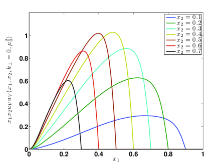
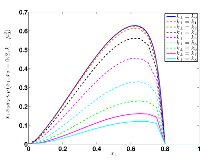
In Fig. 1 the numerical results of the Eqs. (8)-(11) for two unpolarized u𝑢u-valence quarks. The dPDFs vanish in the region x1+x2>1subscript𝑥1subscript𝑥21x_{1}+x_{2}>1 and the correlations in x1,x2subscript𝑥1subscript𝑥2x_{1},x_{2} are dictated by the LF-quark dynamics, which governs also the dependence in ksubscript𝑘perpendicular-tok_{\perp}, clearly seen in the right panel of the same figure. Since the Fock expansion of the proton state has been restricted to the three valence quarks (cfr. Eq. (5)), it is natural that the full momentum is carried by those quarks and the resulting appropriate energy scale remains quite low (the so-called hadronic scale, μ020.1GeV2superscriptsubscript𝜇020.1superscriptGeV2\mu_{0}^{2}\approx 0.1\,{\rm GeV}^{2} [37]) as indicated by analogous LeadingOrder𝐿𝑒𝑎𝑑𝑖𝑛𝑔𝑂𝑟𝑑𝑒𝑟Leading-Order calculations (see, e.g., Refs. [24, 27, 28]). That scale is clearly indicated in the resulting expressions (11) and (12) and in both panels of Fig. 1.

2.3 Factorization and approximations at the low scale of the model

In the present Section we will compare our approach to a number of strategies used in the literature to calculate dPDFs, strategies that we call, in general, ”factorization schemes”. Differences and analogies will help in understanding the role of correlations and their dependence on the evolution scale.

2.3.1 Phenomenological factorizations

As a first illustrative example we can restrict the discussion to the approach proposed by Diehl, Kasements and Keane in Ref. [38], which has motivated in part the discussion presented in this section.
Refer to caption
Refer to caption
Figure 1: Left panel: x1x2uVuV(x1,x2,k=0,μ02)x_{1}x_{2}u_{V}u_{V}(x_{1},x_{2},k_{\perp}=0,\mu_{0}^{2}) as function of x1subscript𝑥1x_{1} at fixed values of x2subscript𝑥2x_{2}. Right panel: x1x2uVuV(x1,x2=0.2,k,μ02)x_{1}x_{2}u_{V}u_{V}(x_{1},x_{2}=0.2,k_{\perp},\mu_{0}^{2}) as function of x1subscript𝑥1x_{1} at various values of ksubscript𝑘perpendicular-tok_{\perp} ( (k0,k1,,k8)(0,0.03,0.14,0.32,0.57,0.85,1.15,1.43,1.68)GeVsimilar-to-or-equalssubscript𝑘0subscript𝑘1subscript𝑘800.030.140.320.570.851.151.431.68GeV(k_{0},k_{1},...,k_{8})\simeq(0,0.03,0.14,0.32,0.57,0.85,1.15,1.43,1.68)\,\,{\rm GeV}, which are Gaussian points between 0 and 2 GeV).

In fact the interest of those authors is on the influence of the evolution scale on correlation effects, precisely one of the goals of the present work. The model they propose refers to the description of the dPDFs at the starting scale, where they assume independent partons. In that case, in fact, the dPDFs in coordinate space can be simply written as a convolution of fa,b(x,b)subscript𝑓𝑎𝑏𝑥𝑏f_{a,b}(x,\vec{b}) functions, which are impact parameter dependent generalized parton distributions (see, e.g, Ref. [3]):

Fab(x1,x2,y)=d2bfa(x1,b+y)fb(x2,b),subscript𝐹𝑎𝑏subscript𝑥1subscript𝑥2𝑦superscript𝑑2𝑏subscript𝑓𝑎subscript𝑥1𝑏𝑦subscript𝑓𝑏subscript𝑥2𝑏F_{ab}(x_{1},x_{2},\vec{y})=\int d^{2}\vec{b}\,f_{a}(x_{1},\vec{b}+\vec{y})f_{b}(x_{2},\vec{b})~{}, (13)

with a,b𝑎𝑏a,b denoting parton species. This idea has been firstly presented in Refs. [32, 33]. The authors of Ref. [38] assume a Gaussian b𝑏\vec{b} dependence with an x𝑥x-dependent width, namely

fa(x,b)=fa(x)14πha(x)exp[b24ha(x)],subscript𝑓𝑎𝑥𝑏subscript𝑓𝑎𝑥14𝜋subscript𝑎𝑥superscript𝑏24subscript𝑎𝑥f_{a}(x,\vec{b})=f_{a}(x){1\over 4\pi h_{a}(x)}\exp{\left[-{\vec{b}^{2}\over 4h_{a}(x)}\right]}~{}, (14)

where fa(x)subscript𝑓𝑎𝑥f_{a}(x) denotes the usual parton densities (taken from the LO set of the MSTW 2008 analysis [39]), while Eq. (14) is assumed to be valid at the starting scale Q02=2subscriptsuperscript𝑄202Q^{2}_{0}=2 GeV2. Diehl et al stress that the approach is tailored for the region x1,x2<0.1subscript𝑥1subscript𝑥20.1x_{1},x_{2}<0.1 and its parameters are specified for gluons and for the sum, q+=q+q¯superscript𝑞𝑞¯𝑞q^{+}=q+\bar{q}, and difference, q=qq¯superscript𝑞𝑞¯𝑞q^{-}=q-\bar{q}, of quark and antiquark distributions. The expressions for ha(x)subscript𝑎𝑥h_{a}(x) are found in Ref. [38] and not reported here; the parameters which are necessary to define ha(x)subscript𝑎𝑥h_{a}(x) are fixed so that the resulting parton densities are in tentative agreement with phenomenology.

The final expression for the unpolarized dPDFs Eq. (13) reads:

Fab(x1,x2,y,Q02)subscript𝐹𝑎𝑏subscript𝑥1subscript𝑥2𝑦superscriptsubscript𝑄02\displaystyle F_{ab}(x_{1},x_{2},\vec{y},Q_{0}^{2}) =\displaystyle= fa(x1,Q02)fb(x2,Q02)14πhab(x1,x2)×\displaystyle f_{a}(x_{1},Q_{0}^{2})f_{b}(x_{2},Q_{0}^{2}){1\over 4\pi h_{ab}(x_{1},x_{2})}\times (15)
×\displaystyle\times exp[y24hab(x1,x2)]superscript𝑦24subscript𝑎𝑏subscript𝑥1subscript𝑥2\displaystyle\exp\left[{-{{\vec{y}}^{2}\over 4h_{ab}(x_{1},x_{2})}}\right]\;\;\;\;\;\;\;\;\;\;\;\;\;\;

and, as a consequence, one has, for the Fourier transform,

Fab(x1,x2,k,Q02)subscript𝐹𝑎𝑏subscript𝑥1subscript𝑥2subscript𝑘perpendicular-tosuperscriptsubscript𝑄02\displaystyle F_{ab}(x_{1},x_{2},k_{\perp},Q_{0}^{2}) =\displaystyle= fa(x1,Q02)fb(x2,Q02)hab(x1,x2)π×\displaystyle f_{a}(x_{1},Q_{0}^{2})f_{b}(x_{2},Q_{0}^{2}){h_{ab}(x_{1},x_{2})\over\pi}\times (16)
×\displaystyle\times exp[hab(x1,x2)k2].subscript𝑎𝑏subscript𝑥1subscript𝑥2superscriptsubscript𝑘perpendicular-to2\displaystyle\exp\left[-h_{ab}(x_{1},x_{2})k_{\perp}^{2}\right].

The term

hab(x1,x2)subscript𝑎𝑏subscript𝑥1subscript𝑥2\displaystyle h_{ab}(x_{1},x_{2}) =\displaystyle= ha(x1)+hb(x2)=subscript𝑎subscript𝑥1subscript𝑏subscript𝑥2absent\displaystyle h_{a}(x_{1})+h_{b}(x_{2})= (17)
=\displaystyle= αaln1x1+αbln1x2+Ba+Bbsubscriptsuperscript𝛼𝑎1subscript𝑥1subscriptsuperscript𝛼𝑏1subscript𝑥2subscript𝐵𝑎subscript𝐵𝑏\displaystyle\alpha^{\prime}_{a}\ln{1\over x_{1}}+\alpha^{\prime}_{b}\ln{1\over x_{2}}+B_{a}+B_{b}\,\;\;\;

is assumed, at the same scale, to introduce correlations between x1subscript𝑥1x_{1} and x2subscript𝑥2x_{2}, in fact Eq. (17) does not factorize into separate contributions from each of the two partons, a𝑎a and b𝑏b (the values of the parameters in Eq. (17) can be found in Ref. [38]). The combinations usuperscript𝑢u^{-} and u+superscript𝑢u^{+} are taken as representatives of the quark sector.

2.3.2 Factorization by means of Generalized Parton Distributions

In Ref. [3], a systematic study of relations between single parton and double parton distributions has been performed. To reduce Fabsubscript𝐹𝑎𝑏F_{ab} to single-particle distributions the authors find it more convenient to work in the transverse-momentum ksubscript𝑘perpendicular-to\vec{k}_{\perp} space, rather than transverse distance y𝑦\vec{y} representation and the result reads:

Fqq(x1,x2,k,Q2)subscript𝐹𝑞𝑞subscript𝑥1subscript𝑥2subscript𝑘perpendicular-tosuperscript𝑄2absent\displaystyle F_{qq}(x_{1},x_{2},\vec{k}_{\perp},Q^{2})\approx
Hq(x1,ξ=0,k2,Q2)Hq(x2,ξ=0,k2,Q2)+\displaystyle\approx H^{q}(x_{1},\xi=0,-k_{\perp}^{2},Q^{2})H^{q}(x_{2},\xi=0,-k_{\perp}^{2},Q^{2})+
+k24Mp2Eq(x1,ξ=0,k2,Q2)Eq(x2,ξ=0,k2,Q2),\displaystyle+\,{k_{\perp}^{2}\over 4M_{p}^{2}}\,E^{q}(x_{1},\xi=0,-k_{\perp}^{2},Q^{2})E^{q}(x_{2},\xi=0,-k_{\perp}^{2},Q^{2})~{},
(18)

where Mpsubscript𝑀𝑝M_{p} is the proton mass and Hq(x,ξ,t)superscript𝐻𝑞𝑥𝜉𝑡H^{q}(x,\xi,t) and Eq(x,ξ,t)superscript𝐸𝑞𝑥𝜉𝑡E^{q}(x,\xi,t) are Generalized Parton Distributions (GPDs) (see, e.g., [40] and references therein). Hqsuperscript𝐻𝑞H^{q} generalize the unpolarized quark densities q(x)𝑞𝑥q(x) while Eqsuperscript𝐸𝑞E^{q} is related to unpolarized quarks in a transversely polarized proton. The first term in Eq. (18) depends on Hqsuperscript𝐻𝑞H^{q} only and it corresponds to the simplest approximation of the two-parton distribution as a product of single-parton distributions (cfr. Eq. (16)).

In Ref. [3] one can read: ”Although the relation between multiparton distributions and GPDs is an approximation whose accuracy is not easy to estimate (and although our current knowledge of GPDs is far less advanced than that of ordinary parton densities) this relation provides opportunities to obtain information about multiple interactions that is hard to get by other means”.

The question on the accuracy is particularly relevant in view of possible experimental studies of multi-parton effects, and the LF-approach we are presenting can shed some light on the approximation (18), including the role played by the E𝐸E correction term. Since GPDs have been studied, precisely within the same LF-approach, by Pasquini, Boffi and Traini [31] some years ago, one can check directly the accuracy of Eq. (18) 333We are indebted to Markus Diehl who brought our attention to Eq. (4.48) of Ref. [3], corresponding to Eq. (18) and for his useful suggestions.. Because of the natural normalization of the expression Eq. (11):

dx1dx2uVuV(x1,x2,k=0,μ02)=2,\int dx_{1}dx_{2}\,u_{V}u_{V}(x_{1},x_{2},k_{\perp}=0,\mu_{0}^{2})=2\,, (19)

and the normalization of the HuVsuperscript𝐻subscript𝑢𝑉H^{u_{V}} GPDs

dxHuV(x,ξ=0,k2)=2,\int dx\,H^{u_{V}}(x,\xi=0,-k_{\perp}^{2})=2\,, (20)
Refer to caption
Refer to caption
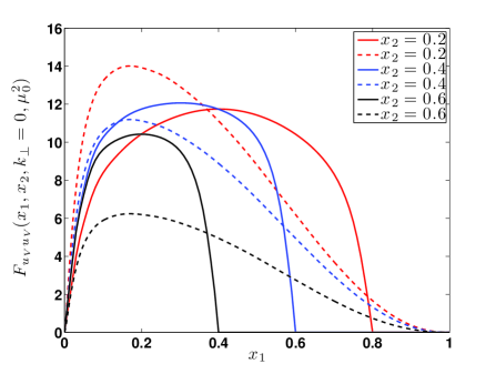
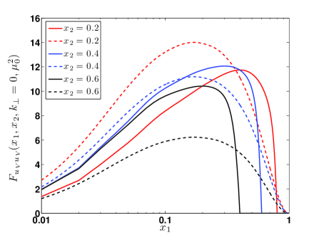
Figure 2: Left panel: FuVuV(x1,x2,k=0,μ02)F_{u_{V}u_{V}}(x_{1},x_{2},k_{\perp}=0,\mu_{0}^{2}) as function of x1subscript𝑥1x_{1} at fixed values of x2=0.2,0.4,0.6subscript𝑥20.20.40.6x_{2}=0.2,0.4,0.6. The continuous lines represent the results obtained within the LF-approach (FuVuV=2×uVuVsubscript𝐹subscript𝑢𝑉subscript𝑢𝑉2subscript𝑢𝑉subscript𝑢𝑉F_{u_{V}u_{V}}=2\times u_{V}u_{V} of Eqs. (8), (11)), the dot-dashed lines the results of the approximation (18). See text for discussion. Right panel: As in the left panel, in logarithmic x𝑥x-scale to emphasized the low-x𝑥x behavior.
Refer to caption
Refer to caption
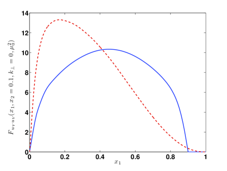
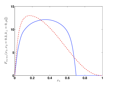
Figure 3: Left panel: FuVuV(x1,x2,k=0,μ02)F_{u_{V}u_{V}}(x_{1},x_{2},k_{\perp}=0,\mu_{0}^{2}) as function x1subscript𝑥1x_{1} at fixed x2=0.1subscript𝑥20.1x_{2}=0.1 and k=0subscript𝑘perpendicular-to0k_{\perp}=0. Right panel: As in the left panel, at fixed x2=0.3subscript𝑥20.3x_{2}=0.3. The continuous line (FuVuV=2×uVuVsubscript𝐹subscript𝑢𝑉subscript𝑢𝑉2subscript𝑢𝑉subscript𝑢𝑉F_{u_{V}u_{V}}=2\times u_{V}u_{V} of Eqs. (8), (11)), crosses the dashed line (approximation (18)) for x10.3subscript𝑥10.3x_{1}\approx 0.3. See text for discussion.
Refer to caption
Refer to caption
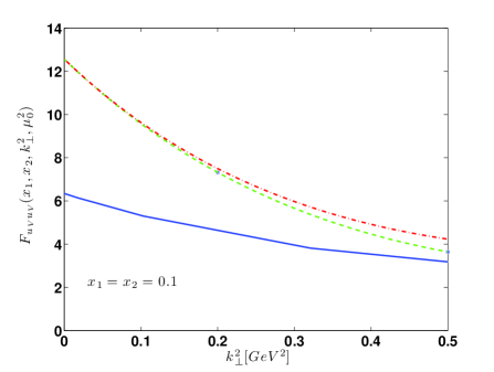
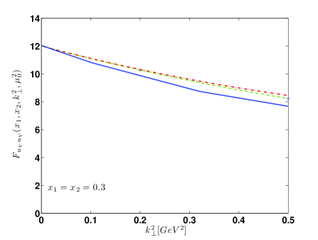
Figure 4: Left panel: FuVuV(x1,x2,k,μ02)subscript𝐹subscript𝑢𝑉subscript𝑢𝑉subscript𝑥1subscript𝑥2subscript𝑘perpendicular-tosuperscriptsubscript𝜇02F_{u_{V}u_{V}}(x_{1},x_{2},k_{\perp},\mu_{0}^{2}) as function of ksubscript𝑘perpendicular-tok_{\perp} at fixed x1=x2=0.1subscript𝑥1subscript𝑥20.1x_{1}=x_{2}=0.1. The continuous line represents the results obtained within the LF-approach (FuVuV=2×uVuVsubscript𝐹subscript𝑢𝑉subscript𝑢𝑉2subscript𝑢𝑉subscript𝑢𝑉F_{u_{V}u_{V}}=2\times u_{V}u_{V} of Eqs. (8), (11)), the dashed lines the results of the approximation (18), the dot-dashed lines neglect the corrections due to the k2superscriptsubscript𝑘perpendicular-to2k_{\perp}^{2}-term in Eq. (18). See text for discussion. Right panel: As in the left panel, at fixed x1=x2=0.3subscript𝑥1subscript𝑥20.3x_{1}=x_{2}=0.3.

the comparison holds for

FuVuV(x1,x2,k,μ02)=2×uVuV(x1,x2,k,μ02)subscript𝐹subscript𝑢𝑉subscript𝑢𝑉subscript𝑥1subscript𝑥2subscript𝑘perpendicular-tosuperscriptsubscript𝜇022subscript𝑢𝑉subscript𝑢𝑉subscript𝑥1subscript𝑥2subscript𝑘perpendicular-tosuperscriptsubscript𝜇02absent\displaystyle F_{u_{V}u_{V}}(x_{1},x_{2},k_{\perp},\mu_{0}^{2})=2\times u_{V}u_{V}(x_{1},x_{2},k_{\perp},\mu_{0}^{2})\approx
HuV(x1,ξ=0,k2,μ02)HuV(x2,ξ=0,k2,μ02)+\displaystyle\approx H^{u_{V}}(x_{1},\xi=0,-k_{\perp}^{2},\mu_{0}^{2})H^{u_{V}}(x_{2},\xi=0,-k_{\perp}^{2},\mu_{0}^{2})+
+k24Mp2EuV(x1,ξ=0,k2,μ02)\displaystyle+\,{k_{\perp}^{2}\over 4M_{p}^{2}}\,E^{u_{V}}(x_{1},\xi=0,-k_{\perp}^{2},\mu_{0}^{2})
EuV(x2,ξ=0,k2,μ02).\displaystyle E^{u_{V}}(x_{2},\xi=0,-k_{\perp}^{2},\mu_{0}^{2})\,.
(21)

Fig. 2 shows a first comparison at k=0subscript𝑘perpendicular-to0k_{\perp}=0, where the correction due to the presence of Eqsuperscript𝐸𝑞E^{q} contributions vanishes. A clear conclusion emerges: the approximations (18) or (21) can have some validity in the restricted regions x1+x2<1subscript𝑥1subscript𝑥21x_{1}+x_{2}<1, the range where the dPDFs do not vanish. For x1+x2>1subscript𝑥1subscript𝑥21x_{1}+x_{2}>1 the dPDFs must vanish while the single parton responses H𝐻H and E𝐸E do not.

A detailed comparison is shown in Fig. 3 and Fig. 4 for two specific values of x2subscript𝑥2x_{2}, namely x2=0.1subscript𝑥20.1x_{2}=0.1 and x2=0.3subscript𝑥20.3x_{2}=0.3. In these two cases the comparison is not restricted to k=0subscript𝑘perpendicular-to0k_{\perp}=0 only (see Fig. 3), but it extends to the kinematical region up to k2=0.5superscriptsubscript𝑘perpendicular-to20.5k_{\perp}^{2}=0.5 GeV2 (see Fig. 4). Once again no systematic agreement is found. The only weak improvement, for k>0subscript𝑘perpendicular-to0k_{\perp}>0, is due to the EuVsuperscript𝐸subscript𝑢𝑉E^{u_{V}} dependent correction term.

3 Scale impact on correlations

Refer to caption
Refer to caption
Refer to caption
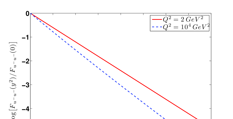
Figure 5: Effects of evolution on correlations according to the scheme of Ref. [38]. Upper panel: ln[Fuu(y2)/Fuu(0)]subscript𝐹superscript𝑢superscript𝑢superscript𝑦2subscript𝐹superscript𝑢superscript𝑢0\ln[F_{u^{-}u^{-}}(\vec{y}^{2})/F_{u^{-}u^{-}}(0)] at x2=x1=0.1subscript𝑥2subscript𝑥10.1x_{2}=x_{1}=0.1 as function of y2superscript𝑦2\vec{y}^{2} [fm2] at fixed values of Q2superscript𝑄2Q^{2} and following the assumptions of Ref. [38]. Middle panel: As in the upper panel for ln[Fu+u+(y2)/Fu+u+(0)]subscript𝐹superscript𝑢superscript𝑢superscript𝑦2subscript𝐹superscript𝑢superscript𝑢0\ln[F_{u^{+}u^{+}}(\vec{y}^{2})/F_{u^{+}u^{+}}(0)]. Lower panel: As previous panels, for ln[Fgg(y2)/Fgg(0)]subscript𝐹𝑔𝑔superscript𝑦2subscript𝐹𝑔𝑔0\ln[F_{gg}(\vec{y}^{2})/F_{gg}(0)].

3.1 Analysis of the approach of Ref. [38]

Let us first analyze the scale dependence of the correlations introduced at Q02superscriptsubscript𝑄02Q_{0}^{2} within the assumptions Eqs. (15) and (16), as proposed by Diehl et al. in Ref. [38]. To this end, we study the QCD-evolution of the dPDFs. In particular one could ask oneself to which extent the Gaussian y𝑦y-dependence (or ksubscript𝑘perpendicular-tok_{\perp}-dependence) of the starting scale is preserved under evolution. Quantities particularly suitable to this end are the ratios

ln[Fab(x1=x2,y2,Q2)Fab(x1=x2,y2=0,Q2)]Q02=y24hab(x1,x2),\ln\left[F_{ab}(x_{1}=x_{2},\vec{y}^{2},Q^{2})\over F_{ab}(x_{1}=x_{2},\vec{y}^{2}=0,Q^{2})\right]_{Q_{0}^{2}}=-{{\vec{y}}^{2}\over 4h_{ab}(x_{1},x_{2})}\,,\\ (22)
ln[Fab(x1=x2,k2,Q2)Fab(x1=x2,k2=0,Q2)]Q02=hab(x1,x2)k2,\ln\left[F_{ab}(x_{1}=x_{2},\vec{k}_{\perp}^{2},Q^{2})\over F_{ab}(x_{1}=x_{2},\vec{k}_{\perp}^{2}=0,Q^{2})\right]_{Q_{0}^{2}}=-{h_{ab}(x_{1},x_{2})\,{\vec{k}_{\perp}}^{2}}\,,\\ (23)

which, at Q02superscriptsubscript𝑄02Q_{0}^{2} and x1=x2=constantsubscript𝑥1subscript𝑥2𝑐𝑜𝑛𝑠𝑡𝑎𝑛𝑡x_{1}=x_{2}=constant, are just straight lines as functions of y2superscript𝑦2\vec{y}^{2} or k2superscriptsubscript𝑘perpendicular-to2k_{\perp}^{2}.

Perturbative evolution of the dPDFs is summarized and discussed in Appendix A; however let us anticipate the results in this example, proposed in Ref. [38]. As it is done also in Ref. [38], only the homogeneus part of dPDFs evolution is implemented, for the moment being, in our scheme. According to some studies, the inhomogeneus part could play some role in this phenomenology [33, 41]; its analysis is beyond the scope of the present paper.

In Fig. 5 we show the ratios Eqs. (22) for different quark and gluon combinations: Fu+u+subscript𝐹superscript𝑢superscript𝑢F_{u^{+}u^{+}}, Fuusubscript𝐹superscript𝑢superscript𝑢F_{u^{-}u^{-}} and Fggsubscript𝐹𝑔𝑔F_{gg} at x1=x2=0.1subscript𝑥1subscript𝑥20.1x_{1}=x_{2}=0.1 at different scales, namely the starting scale Q02=2superscriptsubscript𝑄022Q_{0}^{2}=2 GeV2 and Q2=104superscript𝑄2superscript104Q^{2}=10^{4} GeV2. One can check that, for quarks, the shape remains approximately Gaussian (a straight line) up to scales as high as Q2=104superscript𝑄2superscript104Q^{2}=10^{4} GeV2 even if the slope changes rather strongly. For gluons, also the Gaussian property is not preserved.
Refer to caption
Refer to caption
Refer to caption
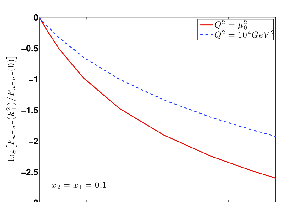
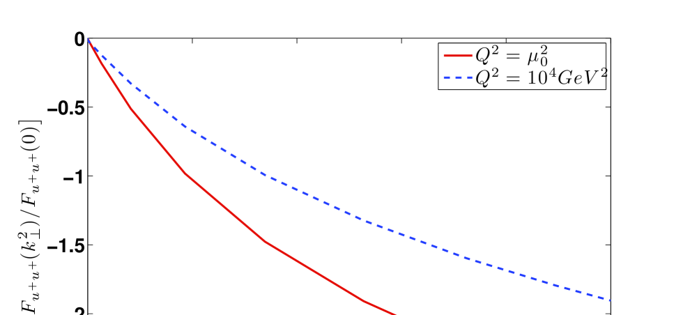
Figure 6: Effects of evolution on correlations for the LF-Hypercentral approach. Upper panel ln[Fuu(k2)/Fuu(0)]subscript𝐹superscript𝑢superscript𝑢superscriptsubscript𝑘perpendicular-to2subscript𝐹superscript𝑢superscript𝑢0\ln[F_{u^{-}u^{-}}(k_{\perp}^{2})/F_{u^{-}u^{-}}(0)] at x2=x1=0.1subscript𝑥2subscript𝑥10.1x_{2}=x_{1}=0.1 as function of k2superscriptsubscript𝑘perpendicular-to2\vec{k}_{\perp}^{2} [fm-2 ] and fixed values of Q2superscript𝑄2Q^{2}. Middle panel: ln[Fu+u+(k2)/Fu+u+(0)]subscript𝐹superscript𝑢superscript𝑢superscriptsubscript𝑘perpendicular-to2subscript𝐹superscript𝑢superscript𝑢0\ln[F_{u^{+}u^{+}}(k_{\perp}^{2})/F_{u^{+}u^{+}}(0)] with analogous notations. Lower panel: ln[Fgg(k2)/Fgg(0)]subscript𝐹𝑔𝑔superscriptsubscript𝑘perpendicular-to2subscript𝐹𝑔𝑔0\ln[F_{gg}(k_{\perp}^{2})/F_{gg}(0)] with the same notations. The gluon distribution Fggsubscript𝐹𝑔𝑔F_{gg} vanishes identically at Q2=μ02superscript𝑄2superscriptsubscript𝜇02Q^{2}=\mu_{0}^{2} (cfr. Eqs. (24)).

In particular the upper panel of Fig. 5 shows the valence components of Fabsubscript𝐹𝑎𝑏F_{ab} (Fuu=F(uu¯)(uu¯)FuVuVsubscript𝐹superscript𝑢superscript𝑢subscript𝐹𝑢¯𝑢𝑢¯𝑢subscript𝐹subscript𝑢𝑉subscript𝑢𝑉F_{u^{-}u^{-}}=F_{(u-\bar{u})(u-\bar{u})}\equiv F_{u_{V}u_{V}}). For those distributions, only the non-singlet evolution is relevant. In the case of Fu+u+=F(u+u¯)(u+u¯)=F(uV+2u¯)(uV+2u¯)=FuVuV+2[FuVu¯+Fu¯uV]+4Fu¯u¯subscript𝐹superscript𝑢superscript𝑢subscript𝐹𝑢¯𝑢𝑢¯𝑢subscript𝐹subscript𝑢𝑉2¯𝑢subscript𝑢𝑉2¯𝑢subscript𝐹subscript𝑢𝑉subscript𝑢𝑉2delimited-[]subscript𝐹subscript𝑢𝑉¯𝑢subscript𝐹¯𝑢subscript𝑢𝑉4subscript𝐹¯𝑢¯𝑢F_{u^{+}u^{+}}=F_{(u+\bar{u})(u+\bar{u})}=F_{(u_{V}+2\bar{u})(u_{V}+2\bar{u})}=F_{u_{V}u_{V}}+2[F_{u_{V}\bar{u}}+F_{\bar{u}u_{V}}]+4F_{\bar{u}\bar{u}} (middle panel), the singlet components are contributing in a substantial way; Fggsubscript𝐹𝑔𝑔F_{gg} (lower panel) is purely singlet. The distributions are defined as functions of the distance |y|𝑦|\vec{y}|, the Fourier transform would give the distributions as functions of ksubscript𝑘perpendicular-to\vec{k}_{\perp} without adding more information. The choice to show the y2superscript𝑦2\vec{y}\,^{2}- dependence makes easier the comparison of the results shown in Fig. 5 with the calculation of Diehl at al. as illustrated in their Figs. 1(a), 1(c), and 1(e).


3.2 Scale dependence within the LF-approach

In the LF-approach the Fock decomposition of the proton state at the lowest scale μ02superscriptsubscript𝜇02\mu_{0}^{2} includes valence quarks only and one remains with the following reductions

Fuusubscript𝐹superscript𝑢superscript𝑢\displaystyle F_{u^{-}u^{-}} \displaystyle\equiv FuVuVsubscript𝐹subscript𝑢𝑉subscript𝑢𝑉\displaystyle F_{u_{V}u_{V}}
\displaystyle\to 2uVuV(x1,x2,k,μ02),2subscript𝑢𝑉subscript𝑢𝑉subscript𝑥1subscript𝑥2subscript𝑘perpendicular-tosuperscriptsubscript𝜇02\displaystyle 2u_{V}u_{V}(x_{1},x_{2},k_{\perp},\mu_{0}^{2})\,,
Fu+u+subscript𝐹superscript𝑢superscript𝑢\displaystyle F_{u^{+}u^{+}} \displaystyle\equiv FuVuV+2[FuVu¯+Fu¯uV]+4Fu¯u¯subscript𝐹subscript𝑢𝑉subscript𝑢𝑉2delimited-[]subscript𝐹subscript𝑢𝑉¯𝑢subscript𝐹¯𝑢subscript𝑢𝑉4subscript𝐹¯𝑢¯𝑢\displaystyle F_{u_{V}u_{V}}+2[F_{u_{V}\bar{u}}+F_{\bar{u}u_{V}}]+4F_{\bar{u}\bar{u}}
\displaystyle\to 2uVuV(x1,x2,k,μ02),2subscript𝑢𝑉subscript𝑢𝑉subscript𝑥1subscript𝑥2subscript𝑘perpendicular-tosuperscriptsubscript𝜇02\displaystyle 2u_{V}u_{V}(x_{1},x_{2},k_{\perp},\mu_{0}^{2})\,,
Fggsubscript𝐹𝑔𝑔\displaystyle F_{gg} \displaystyle\to 0,0\displaystyle 0\,, (24)

with uVuV(x1,x2,k,μ02)subscript𝑢𝑉subscript𝑢𝑉subscript𝑥1subscript𝑥2subscript𝑘perpendicular-tosuperscriptsubscript𝜇02u_{V}u_{V}(x_{1},x_{2},k_{\perp},\mu_{0}^{2}) given by Eqs. (8) and (11).

The distributions are now function of ksubscript𝑘perpendicular-to\vec{k}_{\perp} since in the LF-approach they are defined in momentum space. The relation with y𝑦\vec{y} is a simple Fourier transform (cfr. Eqs. (15) and (16)); however their functional forms, entirely determined by the dynamical structure of the LF-wavefunctions, are far from being Gaussian.

The distributions at the starting point are strongly simplified as indicated by Eqs. (24), but they evolve in a complicated way as combination of non-singlet (Valence=Vi=qiq¯i𝑉𝑎𝑙𝑒𝑛𝑐𝑒subscript𝑉𝑖subscript𝑞𝑖subscript¯𝑞𝑖Valence=V_{i}=q_{i}-\bar{q}_{i}, T3=u+d+subscript𝑇3superscript𝑢superscript𝑑T_{3}=u^{+}-d^{+}, T8=u++d+2s+subscript𝑇8superscript𝑢superscript𝑑2superscript𝑠T_{8}=u^{+}+d^{+}-2s^{+}) as well as singlet components (Σ=u++d++s+=iqi+Σsuperscript𝑢superscript𝑑superscript𝑠subscript𝑖superscriptsubscript𝑞𝑖\Sigma=u^{+}+d^{+}+s^{+}=\sum_{i}q_{i}^{+}, gluons𝑔𝑙𝑢𝑜𝑛𝑠gluons).

In Fig. 6, the results are shown at fixed x2=x1=0.1subscript𝑥2subscript𝑥10.1x_{2}=x_{1}=0.1, Q2=104superscript𝑄2superscript104Q^{2}=10^{4} GeV2, as function of k2superscriptsubscript𝑘perpendicular-to2k_{\perp}^{2}.

The form is clearly non-Gaussian, since non-Gaussian is its functional form at μ02superscriptsubscript𝜇02\mu_{0}^{2}, fact which is related to the dynamics of the LF, not on the value of μ02superscriptsubscript𝜇02\mu_{0}^{2}. The complete results are shown in Fig. 6, following the same notations and criteria of Fig. 5.

Comparing the results of the two set of Figures (5 and 6), it is evident that the evolution effects are similar in the two different cases, but it is also evident that the Gaussian ansatz is rather arbitrary and not supported by LF dynamics.

4 Adding sea quarks and gluons at a low energy scale

In the previous sections, our Light-Front approach has been focused on the study of valence degrees of freedom at low momentum scale. Other partons, and their correlation effects, emerge from radiated gluons in the perturbative QCD-evolution of the dPDFs. In the present Section we enlarge the perspective studying how sea quarks and gluons can be included at a low-momentum scale and within the same LF framework. An example (e.g. Refs. [27, 28]) is given by inclusive DIS, where the (non-perturbative) meson degrees of freedom can be introduced by means of a description of the meson cloud and the scattering of the virtual photon off the constituents of the mesons (Sullivan process). Analogous approach can be applied to the explicit evaluation of meson cloud effects on GPDs (e.g. Refs. [31, 42]).

Hereafter we will propose a simplified approach in which the effects of the valence degrees of freedom (producing the largest part of the dPDFs at low-momentum scale) are calculated using Eqs. (8) and (11), while the non-perturbative sea and gluons components are evaluated by means of a factorized approximation of the kind discussed in Sect. 2.3. In order to minimize the hypothesis on factorization let us start discussing the limiting case k=0subscript𝑘perpendicular-to0k_{\perp}=0. Let us first illustrate, as an example, the uu𝑢𝑢uu dPDFs:

Fuu(x1,x2,k=0,Q02)\displaystyle F_{uu}(x_{1},x_{2},k_{\perp}=0,Q_{0}^{2}) =\displaystyle= F(uV+u¯)(uV+u¯)(x1,x2,k=0,Q02)\displaystyle F_{(u_{V}+\bar{u})(u_{V}+\bar{u})}(x_{1},x_{2},k_{\perp}=0,Q_{0}^{2})
=\displaystyle= FuVuV(x1,x2,k=0,Q02)+\displaystyle F_{u_{V}u_{V}}(x_{1},x_{2},k_{\perp}\!=\!0,Q_{0}^{2})+
+\displaystyle+ [FuVu¯(x1,x2,k=0,Q02)+\displaystyle\left[F_{u_{V}\bar{u}}(x_{1},\!x_{2},k_{\perp}\!=\!0,Q_{0}^{2})+\right.
+\displaystyle+ Fu¯uV(x1,x2,k=0,Q02)]+\displaystyle\left.F_{\bar{u}u_{V}}(x_{1},\!x_{2},k_{\perp}\!=\!0,Q_{0}^{2})\right]+ (26)
+\displaystyle+ Fu¯u¯(x1,x2,k=0,Q02).\displaystyle F_{\bar{u}\bar{u}}(x_{1},x_{2},k_{\perp}=0,Q_{0}^{2})\,. (27)

The pure valence (and dominant) term, the expression (4) in the above equation,

FuVuV(x1,x2,k,Q02)=2×uVuV(x1,x2,k,Q02),subscript𝐹subscript𝑢𝑉subscript𝑢𝑉subscript𝑥1subscript𝑥2subscript𝑘perpendicular-tosuperscriptsubscript𝑄022subscript𝑢𝑉subscript𝑢𝑉subscript𝑥1subscript𝑥2subscript𝑘perpendicular-tosuperscriptsubscript𝑄02F_{u_{V}u_{V}}(x_{1},x_{2},k_{\perp},Q_{0}^{2})=2\times u_{V}u_{V}(x_{1},x_{2},k_{\perp},Q_{0}^{2})\,, (28)

can be evaluated in a direct way within the LF-approach described in the previous sections. In order to calculate the residual terms, Eqs. (26) and (27), one can assume factorized forms (see e.g. Ref. [3]).

The complete (approximate) expression for Fuusubscript𝐹𝑢𝑢F_{uu} becomes:

Fuu(x1,x2,k=0,Q02)\displaystyle F_{uu}(x_{1},x_{2},k_{\perp}\!=\!0,Q_{0}^{2}) \displaystyle\approx (29)
=\displaystyle= FuVuV(x1,x2,k=0,Q02)+\displaystyle F_{u_{V}u_{V}}(x_{1},x_{2},k_{\perp}\!=\!0,Q_{0}^{2})+
+\displaystyle+ {[uV(x1,Q02)u¯(x2,Q02)+u¯(x1,Q02)uV(x2,Q02)]+\displaystyle\left\{\left[u_{V}(x_{1},Q_{0}^{2})\bar{u}(x_{2},Q_{0}^{2})+\bar{u}(x_{1},Q_{0}^{2})u_{V}(x_{2},Q_{0}^{2})\right]+\right.
+\displaystyle+ u¯(x1,Q02)u¯(x2,Q02)}(1x1x2)nθ(1x1x2).\displaystyle\left.\bar{u}(x_{1},Q_{0}^{2})\bar{u}(x_{2},Q_{0}^{2})\right\}(1-x_{1}-x_{2})^{n}\theta(1-x_{1}-x_{2})\,.

Few comments are in order:

  • i)

    the contribution Eq. (4) is the term due to valence quarks, it is not approximated by a factorized procedure and it is based on the calculated expressions Eqs. (8) and (11);

  • ii)

    the residual contributions imply the knowledge of the singlet component u¯(x,Q02)¯𝑢𝑥superscriptsubscript𝑄02\bar{u}(x,Q_{0}^{2}) and fulfill the correct kinematical conditions for x1+x2>1subscript𝑥1subscript𝑥21x_{1}+x_{2}>1, owing to the constraints introduced by the phenomenological function (1x1x2)nθ(1x1x2)superscript1subscript𝑥1subscript𝑥2𝑛𝜃1subscript𝑥1subscript𝑥2(1-x_{1}-x_{2})^{n}\theta(1-x_{1}-x_{2}). The exponent n𝑛n has to be fixed phenomenologically, as seen in Sect. 2.3.1 in the case of the model of Ref. [38] and will be discussed in the next Sections for the LF-approach;

  • iii)

    u¯(x,Q02)=usea(x,Q02)¯𝑢𝑥superscriptsubscript𝑄02subscript𝑢𝑠𝑒𝑎𝑥superscriptsubscript𝑄02\bar{u}(x,Q_{0}^{2})=u_{sea}(x,Q_{0}^{2}) has, at the low momentum scale Q02superscriptsubscript𝑄02Q_{0}^{2}, a non-perturbative origin, basically due to the meson cloud surrounding the nucleon;

  • iv)

    the scale Q02superscriptsubscript𝑄02Q_{0}^{2} is not to be identified with μ02superscriptsubscript𝜇02\mu_{0}^{2}, i.e. the scale of the bare nucleon, where only the three valence quarks contribute.

In the following sections we will discuss a straight-forward (phenomenological) way of introducing meson and gluon degrees of freedom at the low-momentum non-perturbative scale. QCD evolution will be used to reach the high energy scale of the LHC experiments.

4.1 Factorization procedures within the LF-approach at k=0subscript𝑘perpendicular-to0k_{\perp}=0

The advantage of the approach we are discussing is based on a complete calculation of correlation effects within the LF-dynamics, in the restricted space of valence degrees of freedom. At the same time it allows to discuss the role of the factorization procedure and its validity, comparing our approach with phenomenological factorized models. This comparison aims to identify the coherence and self-consistency of the factorization schemes. In the following we will give three examples: i) the identification of the exponent n𝑛n to fix the correlating function Eq. (LABEL:eq:correlationQ0) [see Sect. 4.1.1]; ii) the introduction of a larger number of degrees of freedom at k=0subscript𝑘perpendicular-to0k_{\perp}=0 [Sect. 4.1.2]; iii) the extension to k>0subscript𝑘perpendicular-to0k_{\perp}>0 of the sea and gluon contributions to dPDFs [Sect. 4.2].

4.1.1 Fixing the factorization form

The optimization of factorization procedures for dPDFs is not a simple issue. The most relevant constraints are related to momentum and quark number sum rules [2]. Our LF-approach, on the contrary, fulfills such sum rules by construction and therefore one does not need to implement phenomenological assumptions required to build factorized dPDFs.

As an example the resulting valence dPDF uVuV(x1,x2,k=0,μ02)u_{V}u_{V}(x_{1},x_{2},k_{\perp}=0,\mu_{0}^{2}), as well as the single PDFs (sPDFs) calculated within the same LF dynamical approach, fulfill the momentum and quark number sum rules. One can take advantage from such fundamental properties to fix the order of magnitude of the phenomenological exponent n𝑛n in Eq. (LABEL:eq:correlationQ0), trying to combine the knowledge of sPDFs and dPDFs in the following (factorized) relation:

FuVuV(x1,x2,k=0,μ02)=\displaystyle F_{u_{V}u_{V}}(x_{1},x_{2},k_{\perp}=0,\mu_{0}^{2})= (32)
=\displaystyle= 2uVuV(x1,x2,k=0,μ02)|LF=\displaystyle\left.2\cdot u_{V}u_{V}(x_{1},x_{2},k_{\perp}=0,\mu_{0}^{2})\right|_{\rm LF}=
\displaystyle\approx uV(x1,μ02)|LFuV(x1,μ02)|LF×\displaystyle\left.\left.u_{V}(x_{1},\mu_{0}^{2})\right|_{\rm LF}u_{V}(x_{1},\mu_{0}^{2})\right|_{\rm LF}\times
×\displaystyle\times (1x1x2)nθ(1x1x2).superscript1subscript𝑥1subscript𝑥2𝑛𝜃1subscript𝑥1subscript𝑥2\displaystyle(1-x_{1}-x_{2})^{n}\theta(1-x_{1}-x_{2})\,.

The restricted validity of the factorization approach has been already discussed in Sect. 2.3, therefore one cannot expect Eq. (32) to be satisfied with a high degree of accuracy. We expect, however, indications for the value of the exponent n𝑛n to be used for building the additional sea and gluon contributions to the dPDFs. The value n=2𝑛2n=2 has been discussed in the past as a good choice (see, e.g., Ref. [43] and references therein). More recent arguments (see, e.g., Refs. [38], and [2]) are in favor of more sophisticated parametrizations. Given the restricted use we are going to make of the factorization assumption, we prefer to remain within the straight-forward formulation Eq. (32). Our numerical analysis confirms a limited validity of the factorization and, at the same time, suggests n0.2𝑛0.2n\approx 0.2 (more precisely, values within the range 0.1<n<0.50.1𝑛0.50.1<n<0.5; n=0.2𝑛0.2n=0.2 is our optimal choice).

4.1.2 Sea and gluon contribution according to Ref. [39]

The advantages of the approximation Eq. (29) are now clear: the largest contributions are due to the valence components and the LF approach has the merit of preserving at μ02superscriptsubscript𝜇02\mu_{0}^{2} quark number and momentum sum rules. The perturbative evolution needed to reach the new low-momentum scale Q02superscriptsubscript𝑄02Q_{0}^{2} to integrate new degrees of freedom preserves those constraints. At the same time the residual terms can be approximated within a clear and self constrained factorized approach able to select the form of the factorization as discussed in the previous subsection.

In the following we discuss the introduction of sea and gluon degrees of freedom by means of one of the most used phenomenological parametrization of sPDF, the LO𝐿𝑂LO MSTW2008 parametrization (see Table 4 of Ref. [39]). The parametrization is valid at Q02=1.0superscriptsubscript𝑄021.0Q_{0}^{2}=1.0 GeV2. The fact that we are proposing LO𝐿𝑂LO parametrization is specifically due to the evolution properties of the dPDFs, known at LO𝐿𝑂LO only.

Refer to caption
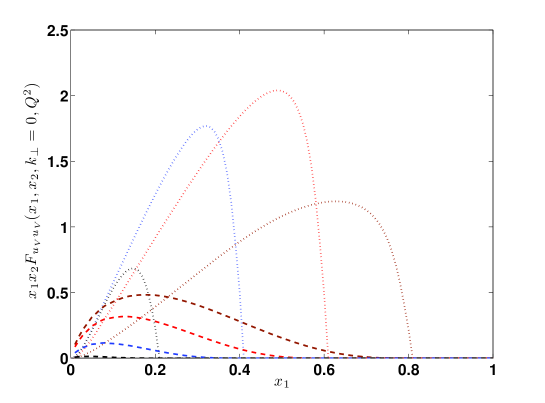
Figure 7: x1x2FuVuV(x1,x2,k=0,Q2)x_{1}x_{2}F_{u_{V}u_{V}}(x_{1},x_{2},k_{\perp}=0,Q^{2}) as function of x1subscript𝑥1x_{1} and x2=0,2,0.4,0.6,0.8subscript𝑥2020.40.60.8x_{2}=0,2,0.4,0.6,0.8 and for two values of Q2superscript𝑄2Q^{2}, namely the extreme low momentum scale μ02superscriptsubscript𝜇02\mu_{0}^{2} (dotted lines) and the scale (dashed lines) of the MSTW parametrization, Q2=Q02=1.0superscript𝑄2superscriptsubscript𝑄021.0Q^{2}=Q_{0}^{2}=1.0 GeV2.

At the scale Q02superscriptsubscript𝑄02Q_{0}^{2} , the sPDF MSTW2008 parametrization is characterized by the presence of partons like uVsubscript𝑢𝑉u_{V}, dVsubscript𝑑𝑉d_{V}, u¯¯𝑢\bar{u}, d¯¯𝑑\bar{d}, s𝑠s, s¯¯𝑠\bar{s} and gluons𝑔𝑙𝑢𝑜𝑛𝑠gluons. The total momentum is shared among such degrees of freedom and one has:

𝑑xx[uV(x,Q02)+dV(x,Q02)]=0.452;differential-d𝑥𝑥delimited-[]subscript𝑢𝑉𝑥superscriptsubscript𝑄02subscript𝑑𝑉𝑥superscriptsubscript𝑄020.452\displaystyle\int dx\,x\,\left[u_{V}(x,Q_{0}^{2})+d_{V}(x,Q_{0}^{2})\right]=0.452\,; (33)
𝑑xxSea(x,Q02)differential-d𝑥𝑥𝑆𝑒𝑎𝑥superscriptsubscript𝑄02\displaystyle\int dx\,x\,Sea(x,Q_{0}^{2}) =\displaystyle= dxx[(2u¯(x,Q02)+2d¯(x,Q02))\displaystyle\int dx\,x\,\left[(2\bar{u}(x,Q_{0}^{2})+2\bar{d}(x,Q_{0}^{2}))\right. (34)
+\displaystyle+ s(x,Q02)+s¯(x,Q02)]=0.108\displaystyle\left.s(x,Q_{0}^{2})+\bar{s}(x,Q_{0}^{2})\right]=0.108\,
𝑑xxg(x,Q02)=0.431.differential-d𝑥𝑥𝑔𝑥superscriptsubscript𝑄020.431\displaystyle\int dx\,x\,g(x,Q_{0}^{2})=0.431\,. (35)

Since at the scale μ02superscriptsubscript𝜇02\mu_{0}^{2} the system is determined by the valence degrees of freedom only, one has: 𝑑xx[uV(x,μ02)+dV(x,μ02)]=1differential-d𝑥𝑥delimited-[]subscript𝑢𝑉𝑥superscriptsubscript𝜇02subscript𝑑𝑉𝑥superscriptsubscript𝜇021\int dxx\left[u_{V}(x,\mu_{0}^{2})+d_{V}(x,\mu_{0}^{2})\right]\!\!=\!\!1; Sea(x,μ02)=0𝑆𝑒𝑎𝑥superscriptsubscript𝜇020Sea(x,\mu_{0}^{2})\!=\!0; g(x,μ02)=0𝑔𝑥superscriptsubscript𝜇020g(x,\mu_{0}^{2})=0. As a consequence, to use Eq. (32) at the scale Q02superscriptsubscript𝑄02Q_{0}^{2}, the dPDF uVuV(x1,x2,k=0,μ02)u_{V}u_{V}(x_{1},x_{2},k_{\perp}=0,\mu_{0}^{2}) at the scale μ02superscriptsubscript𝜇02\mu_{0}^{2} has to be evolved to Q02superscriptsubscript𝑄02Q_{0}^{2}. The evolution is performed by means of the Non-Singlet reduction of the QCD evolution as described in Ref. [14] and summarized in the appendix A, where the complete Mellin procedure we are proposing for both Singlet and Non-Singlet sectors is illustrated in some detail. The result is shown in Fig. 7 for four selected values of x2subscript𝑥2x_{2}.

Refer to caption
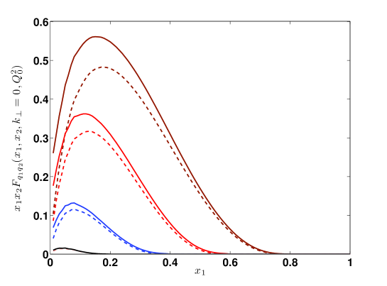
Figure 8: x1x2FuVuV(x1,x2,k=0,Q02)x_{1}x_{2}F_{u_{V}u_{V}}(x_{1},x_{2},k_{\perp}=0,Q_{0}^{2}) (dashed lines) of Fig. 7 is compared with x1x2Fuu(x1,x2,k=0,Q02)x_{1}x_{2}F_{uu}(x_{1},x_{2},k_{\perp}=0,Q_{0}^{2}) which contains the additional sea contributions from u¯¯𝑢\bar{u} (u=uV+u¯𝑢subscript𝑢𝑉¯𝑢u=u_{V}+\bar{u}, see text) (continuous lines).
Refer to caption
Figure 9: The dPDFs (at Q02superscriptsubscript𝑄02Q_{0}^{2} and k=0subscript𝑘perpendicular-to0k_{\perp}=0) due to the interference of u𝑢u quarks and gluons as function of x1subscript𝑥1x_{1} and selected values of x2subscript𝑥2x_{2}.

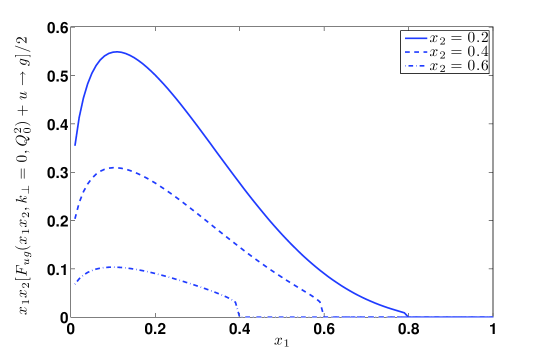
In Fig. 8 and Fig. 9 we show the complete set of dPDFs involving the u𝑢u-quark at the starting scale Q02superscriptsubscript𝑄02Q_{0}^{2}. In particular, the combination Fuu=F(uV+u¯)(uV+u¯)=FuVuV+[FuVu¯+Fu¯uV]+Fu¯u¯subscript𝐹𝑢𝑢subscript𝐹subscript𝑢𝑉¯𝑢subscript𝑢𝑉¯𝑢subscript𝐹subscript𝑢𝑉subscript𝑢𝑉delimited-[]subscript𝐹subscript𝑢𝑉¯𝑢subscript𝐹¯𝑢subscript𝑢𝑉subscript𝐹¯𝑢¯𝑢F_{uu}=F_{(u_{V}+\bar{u})(u_{V}+\bar{u})}=F_{u_{V}u_{V}}+[F_{u_{V}\bar{u}}+F_{\bar{u}u_{V}}]+F_{\bar{u}\bar{u}} is shown in Fig. 8 giving explicit evidence to the contribution due to u¯¯𝑢\bar{u} quarks. The largest effects of the sea component are clearly evident for smallest values of the momentum fraction. In Fig. 9 we show the dPDFs (Fug+Fgu)/2subscript𝐹𝑢𝑔subscript𝐹𝑔𝑢2(F_{ug}+F_{gu})/2 containing valence, sea and gluon contributions. The order of magnitude of those components is comparable with the valence part FuVuVsubscript𝐹subscript𝑢𝑉subscript𝑢𝑉F_{u_{V}u_{V}} at the scale Q02superscriptsubscript𝑄02Q_{0}^{2} (cfr. Fig. 7).

4.2 Factorization procedures within the LF-approach at k>0subscript𝑘perpendicular-to0k_{\perp}>0

The dPDFs in a pure valence scenario have been discussed in previous sections and the dependence on ksubscript𝑘perpendicular-tok_{\perp} has been explicitly investigated (cfr. for example, Figs. 1, 4, and 6). As a result they do not admit simple factorized forms. However, as a first attempt to go beyond the valence scenario at k0subscript𝑘perpendicular-to0k_{\perp}\neq 0, we could add the other degrees of freedom using factorized expressions. To this aim, the knowledge of the exact LF valence component at k=0subscript𝑘perpendicular-to0k_{\perp}=0 helps to define the additional, factorized contributions. In this section we find a reasonable factorized approximation to the exact valence LF dPDFs. In this way we fix the parameters which will be used for the non-valence degrees of freedom

In practice, we want to generalize to k>0subscript𝑘perpendicular-to0k_{\perp}>0 Eqs. (LABEL:eq:correlationQ0) and (32), valid at k=0subscript𝑘perpendicular-to0k_{\perp}=0. For instance, Eq. (32) becomes

FuVuV(x1,x2,k,μ02)=subscript𝐹subscript𝑢𝑉subscript𝑢𝑉subscript𝑥1subscript𝑥2subscript𝑘perpendicular-tosuperscriptsubscript𝜇02absent\displaystyle F_{u_{V}u_{V}}(x_{1},x_{2},k_{\perp},\mu_{0}^{2})= (36)
=\displaystyle= 2uVuV(x1,x2,k,μ02)|LFevaluated-at2subscript𝑢𝑉subscript𝑢𝑉subscript𝑥1subscript𝑥2subscript𝑘perpendicular-tosuperscriptsubscript𝜇02LFabsent\displaystyle\left.2\cdot u_{V}u_{V}(x_{1},x_{2},k_{\perp},\mu_{0}^{2})\right|_{\rm LF}\approx
\displaystyle\approx uV(x1,μ02)|LFuV(x1,μ02)|LF×\displaystyle\left.\left.u_{V}(x_{1},\mu_{0}^{2})\right|_{\rm LF}u_{V}(x_{1},\mu_{0}^{2})\right|_{\rm LF}\times
×\displaystyle\times (1x1x2)nϕ(x1,x2,k)θ(1x1x2),superscript1subscript𝑥1subscript𝑥2𝑛italic-ϕsubscript𝑥1subscript𝑥2subscript𝑘perpendicular-to𝜃1subscript𝑥1subscript𝑥2\displaystyle\left(1-x_{1}-x_{2}\right)^{n}\,\phi(x_{1},x_{2},k_{\perp})\,\theta(1-x_{1}-x_{2})\,,

and simple choices are (cfr. Eq. (16)),

A)\displaystyle A)\;\;\; ϕA(k)=exp[bA2k2],subscriptitalic-ϕ𝐴subscript𝑘perpendicular-tosuperscriptsubscript𝑏𝐴2superscriptsubscript𝑘perpendicular-to2\displaystyle\phi_{A}(k_{\perp})=\exp\left[-b_{A}^{2}\,k_{\perp}^{2}\right]\,, (37)
B)\displaystyle B)\;\;\; ϕB(x1,x2,k)=subscriptitalic-ϕ𝐵subscript𝑥1subscript𝑥2subscript𝑘perpendicular-toabsent\displaystyle\phi_{B}(x_{1},x_{2},k_{\perp})= (38)
=\displaystyle= exp[bB2(1x1x2)nk2].superscriptsubscript𝑏𝐵2superscript1subscript𝑥1subscript𝑥2𝑛superscriptsubscript𝑘perpendicular-to2\displaystyle\exp\left[-b_{B}^{2}\,(1-x_{1}-x_{2})^{n}k_{\perp}^{2}\right]\,.

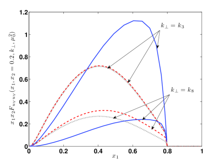
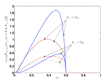
Within scenario A𝐴A of Eq. (37), no correlations between x1,x2subscript𝑥1subscript𝑥2x_{1},x_{2} and ksubscript𝑘perpendicular-tok_{\perp} have been introduced: ϕAsubscriptitalic-ϕ𝐴\phi_{A} depends on ksubscript𝑘perpendicular-tok_{\perp} and it does not depend on x1,x2subscript𝑥1subscript𝑥2x_{1},x_{2}; in scenario B𝐵B of Eq. (38) the exponent depends on x1,x2subscript𝑥1subscript𝑥2x_{1},x_{2}, similarly to Eq. (16). The knowledge of uVuV(x1,x2,k,μ02)|LFevaluated-atsubscript𝑢𝑉subscript𝑢𝑉subscript𝑥1subscript𝑥2subscript𝑘perpendicular-tosuperscriptsubscript𝜇02LF\left.u_{V}u_{V}(x_{1},x_{2},k_{\perp},\mu_{0}^{2})\right|_{\rm LF} from Eq. (11) and of the sPDF uV(x1,μ02)|LFevaluated-atsubscript𝑢𝑉subscript𝑥1superscriptsubscript𝜇02LF\left.u_{V}(x_{1},\mu_{0}^{2})\right|_{\rm LF} with the additional information n=0.2𝑛0.2n=0.2 from the analysis of Sect. 4.1.1, can be used to optimize the fit Eq. (36). The results of the optimization procedure are shown in Fig. 10 for selected and extreme examples. Our recommended values are bA=bB=0.6subscript𝑏𝐴subscript𝑏𝐵0.6b_{A}=b_{B}=0.6 GeV-1 and the quality of the fit is, once again, quite poor with a slight preference for the full correlated approximation of scenario B𝐵B (Eq.(38)). The approximation is crude for the valence-valence correlations, but it is sound and the next subsection will be devoted to the implementation of additional degrees of freedom on the basis offered by the factorization Eq. (36) and scenario B𝐵B.

Refer to caption
Refer to caption
Figure 10: The exact LF dPDFs x1x2FuVuV(x1,x2,k,μ02)subscript𝑥1subscript𝑥2subscript𝐹subscript𝑢𝑉subscript𝑢𝑉subscript𝑥1subscript𝑥2subscript𝑘perpendicular-tosuperscriptsubscript𝜇02x_{1}x_{2}F_{u_{V}u_{V}}(x_{1},x_{2},k_{\perp},\mu_{0}^{2}) (continous lines) and its factorized approximation Eq. (36) (scenario B𝐵B Eq. (38) , dashed lines, scenario A𝐴A Eq. (37), dotted, almost indistinguishable for k=k3subscript𝑘perpendicular-tosubscript𝑘3k_{\perp}=k_{3}), as function of x1subscript𝑥1x_{1} at x2=0.2subscript𝑥20.2x_{2}=0.2 (left panel) and x2=0.4subscript𝑥20.4x_{2}=0.4 (right panel); k3=0.32subscript𝑘30.32k_{3}=0.32 GeV and k8=1.68subscript𝑘81.68k_{8}=1.68 GeV (cfr. the caption of Fig. 1). We remind that n=0.2𝑛0.2n=0.2 and bA=bB=0.6subscript𝑏𝐴subscript𝑏𝐵0.6b_{A}=b_{B}=0.6 GeV-1 (see text).

4.2.1 Sea and gluon contribution at k>0subscript𝑘perpendicular-to0k_{\perp}>0

The valence-valence dPDFs do not allow for a simple factorization. The approximation proposed in Eq. (36) is therefore quite poor in that case, as Fig. 10 explicitly shows. However, we do not need to approximate valence-valence correlations; we can resort to the exact calculation also in the case of k>0subscript𝑘perpendicular-to0k_{\perp}>0 (cfr. Fig. 1 and Eqs. (8), (11)) and, using the best factorization scheme (n=0.2𝑛0.2n=0.2 and bA=bB=0.6subscript𝑏𝐴subscript𝑏𝐵0.6b_{A}=b_{B}=0.6 GeV-1 in Eqs. (37), (38)) to introduce the additional degrees of freedom at the scale Q02superscriptsubscript𝑄02Q_{0}^{2} and k>0subscript𝑘perpendicular-to0k_{\perp}>0. We have to follow once again the steps i)-iv) of Sect. 4 and the procedure described in Sect. 4.1.2. Numerically they are more challenging and, in a sense, incomplete since the evolution in ksubscript𝑘perpendicular-tok_{\perp} is still an open problem [3]. We simply evolve at fixed ksubscript𝑘perpendicular-tok_{\perp} applying the scale evolution of Appendix A.
Refer to caption
Refer to caption
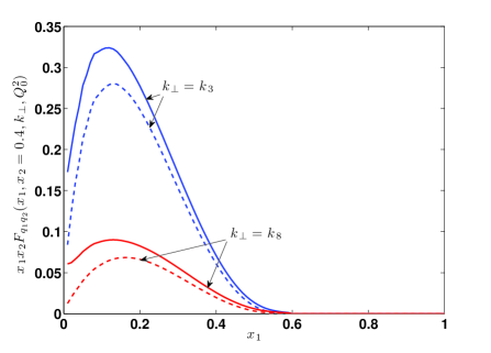
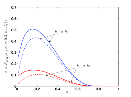
Figure 11: The exact LF dPDFs x1x2FuVuV(x1,x2,k,Q02)subscript𝑥1subscript𝑥2subscript𝐹subscript𝑢𝑉subscript𝑢𝑉subscript𝑥1subscript𝑥2subscript𝑘perpendicular-tosuperscriptsubscript𝑄02x_{1}x_{2}F_{u_{V}u_{V}}(x_{1},x_{2},k_{\perp},Q_{0}^{2}) (Eq.(4.2.1), dashed lines lines) as function of x1subscript𝑥1x_{1} and at fixed x2=0.2subscript𝑥20.2x_{2}=0.2 (left panel) and x2=0.4subscript𝑥20.4x_{2}=0.4 (right panel). x1x2Fuu(x1,x2,k,Q02)subscript𝑥1subscript𝑥2subscript𝐹𝑢𝑢subscript𝑥1subscript𝑥2subscript𝑘perpendicular-tosuperscriptsubscript𝑄02x_{1}x_{2}F_{uu}(x_{1},x_{2},k_{\perp},Q_{0}^{2}) (continuos lines) are obtained from the expression (39) and scenario B𝐵B Eq. (38); k3=0.32subscript𝑘30.32k_{3}=0.32 GeV and k8=1.68subscript𝑘81.68k_{8}=1.68 GeV (cfr. the caption of Fig. 1).

As an example we show in Fig. 11 the distribution Fuu(x1,x2,k,Q02)subscript𝐹𝑢𝑢subscript𝑥1subscript𝑥2subscript𝑘perpendicular-tosuperscriptsubscript𝑄02F_{uu}(x_{1},x_{2},k_{\perp},Q_{0}^{2}) at the scale Q02superscriptsubscript𝑄02Q_{0}^{2} which generalizes Eq. (LABEL:eq:correlationQ0) and Fig. 8, and whose resulting expression reads (from now on, we will discuss the scenario B𝐵B of Eq. (38) only):

Fuu(x1,x2,k,Q02)subscript𝐹𝑢𝑢subscript𝑥1subscript𝑥2subscript𝑘perpendicular-tosuperscriptsubscript𝑄02\displaystyle F_{uu}(x_{1},x_{2},k_{\perp},Q_{0}^{2}) \displaystyle\approx (39)
=\displaystyle= 2uVuV(x1,x2,k,Q02)+limit-from2subscript𝑢𝑉subscript𝑢𝑉subscript𝑥1subscript𝑥2subscript𝑘perpendicular-tosuperscriptsubscript𝑄02\displaystyle 2\cdot u_{V}u_{V}(x_{1},x_{2},k_{\perp},Q_{0}^{2})+
+\displaystyle+ {[uV(x1,Q02)u¯(x2,Q02)+uV(x2,Q02)u¯(x1,Q02)]+\displaystyle\left\{\left[u_{V}(x_{1},Q_{0}^{2})\bar{u}(x_{2},Q_{0}^{2})+u_{V}(x_{2},Q_{0}^{2})\bar{u}(x_{1},Q_{0}^{2})\right]+\right.
+\displaystyle+ u¯(x1,Q02)u¯(x2,Q02)}(1x1x2)n×\displaystyle\left.\bar{u}(x_{1},Q_{0}^{2})\bar{u}(x_{2},Q_{0}^{2})\right\}(1-x_{1}-x_{2})^{n}\times
×\displaystyle\times ϕB(x1,x2,k)θ(1x1x2);subscriptitalic-ϕ𝐵subscript𝑥1subscript𝑥2subscript𝑘perpendicular-to𝜃1subscript𝑥1subscript𝑥2\displaystyle\phi_{B}(x_{1},x_{2},k_{\perp})\,\,\theta(1-x_{1}-x_{2})\,; (41)
Refer to caption
Refer to caption
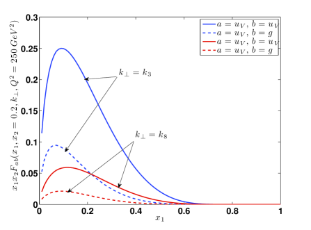
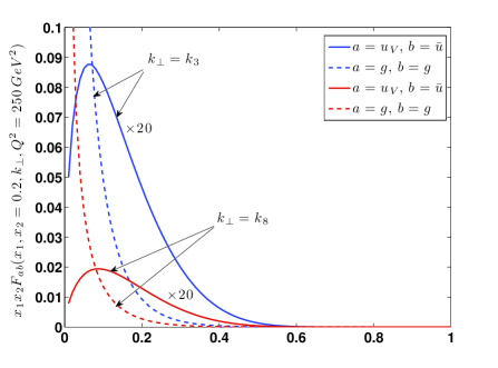
Figure 12: Left panel: The x1x2FuVuVsubscript𝑥1subscript𝑥2subscript𝐹subscript𝑢𝑉subscript𝑢𝑉x_{1}x_{2}F_{u_{V}u_{V}} dPDFs obtained from perturbative evolution from the lowest scale μ02superscriptsubscript𝜇02\mu_{0}^{2} to Q2=250superscript𝑄2250Q^{2}=250 GeV2 (continuous lines) as function of x1subscript𝑥1x_{1} and at fixed x2=0.2subscript𝑥20.2x_{2}=0.2 (and for two values of ksubscript𝑘perpendicular-tok_{\perp}), are compared with x1x2FuVgsubscript𝑥1subscript𝑥2subscript𝐹subscript𝑢𝑉𝑔x_{1}x_{2}F_{u_{V}g} dPDFs (dashed lines) at the same high scale. Right panel: The x1x2FuVu¯subscript𝑥1subscript𝑥2subscript𝐹subscript𝑢𝑉¯𝑢x_{1}x_{2}F_{u_{V}\bar{u}} dPDFs (amplified 20 times) at the scale Q2=250superscript𝑄2250Q^{2}=250 GeV2 are compared with the x1x2Fggsubscript𝑥1subscript𝑥2subscript𝐹𝑔𝑔x_{1}x_{2}F_{gg} dPDFs at the same scale, and kinematical conditions. (k30.32similar-to-or-equalssubscript𝑘30.32k_{3}\simeq 0.32 GeV and k81.68similar-to-or-equalssubscript𝑘81.68k_{8}\simeq 1.68 GeV).
Refer to caption
Refer to caption
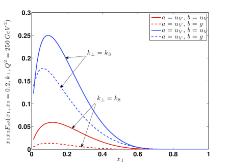
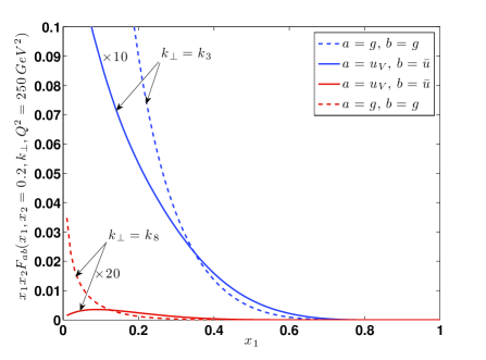
Figure 13: Left panel: The x1x2FuVuVsubscript𝑥1subscript𝑥2subscript𝐹subscript𝑢𝑉subscript𝑢𝑉x_{1}x_{2}F_{u_{V}u_{V}} dPDFs obtained from perturbative evolution from the Q02superscriptsubscript𝑄02Q_{0}^{2} scale to Q2=250superscript𝑄2250Q^{2}=250 GeV2 (continuous lines) as function of x1subscript𝑥1x_{1} and at fixed x2=0.2subscript𝑥20.2x_{2}=0.2 (and for two values of ksubscript𝑘perpendicular-tok_{\perp}), are compared with x1x2FuVgsubscript𝑥1subscript𝑥2subscript𝐹subscript𝑢𝑉𝑔x_{1}x_{2}F_{u_{V}g} dPDFs (dashed lines) at the same high scale. Right panel: The x1x2FuVu¯subscript𝑥1subscript𝑥2subscript𝐹subscript𝑢𝑉¯𝑢x_{1}x_{2}F_{u_{V}\bar{u}} dPDFs (amplified 10 and 20 times respectively) at the scale Q2=250superscript𝑄2250Q^{2}=250 GeV2 are compared with the x1x2Fggsubscript𝑥1subscript𝑥2subscript𝐹𝑔𝑔x_{1}x_{2}F_{gg} correlations at the same scale, and kinematical conditions. (k30.32similar-to-or-equalssubscript𝑘30.32k_{3}\simeq 0.32 GeV and k81.68similar-to-or-equalssubscript𝑘81.68k_{8}\simeq 1.68 GeV). The only difference of the present Figure with Fig. 12 is represented by the starting scale Q02=1.0superscriptsubscript𝑄021.0Q_{0}^{2}=1.0 GeV 22\!\!{}^{2} >μ02absentsuperscriptsubscript𝜇02>\mu_{0}^{2}. As a consistency check one can verify that the results obtained in the two Figures for x1x2FuVuVsubscript𝑥1subscript𝑥2subscript𝐹subscript𝑢𝑉subscript𝑢𝑉x_{1}x_{2}F_{u_{V}u_{V}} are exactly the same. See text.

where uVuV(x1,x2,k,Q02)subscript𝑢𝑉subscript𝑢𝑉subscript𝑥1subscript𝑥2subscript𝑘perpendicular-tosuperscriptsubscript𝑄02u_{V}u_{V}(x_{1},x_{2},k_{\perp},Q_{0}^{2}) is obtained evolving at the scale of the MSTW parametrization, Q02=1.0superscriptsubscript𝑄021.0Q_{0}^{2}=1.0 GeV2, the LF result (8), (11) at fixed ksubscript𝑘perpendicular-tok_{\perp}. Besides, uV(x,Q02)subscript𝑢𝑉𝑥superscriptsubscript𝑄02u_{V}(x,Q_{0}^{2}) is the PDF obtained at the same scale within the LF approach, and u¯(x,Q02)¯𝑢𝑥superscriptsubscript𝑄02\bar{u}(x,Q_{0}^{2}) is taken from the LO MSTW parametrization [39].

By means of the perturbative evolution developed in Appendix A one can now evolve the distribution calculated at low-momentum scale to a typical experimental scale. We evolve to Q2=250superscript𝑄2250Q^{2}=250 GeV2, a scale relevant to study properties of dPDFs, as shown by experiments [17, 18, 19, 20, 21, 22] and by a quite recent theoretical study within the LF approach [23]. In two series of figures, (Figs. 12 and 13), we compare the results obtained evolving directly from the lowest scale μ02superscriptsubscript𝜇02\mu_{0}^{2} where only valence-valence dPDFs are present (cfr. Fig. 1), with those obtained with the evolution from the scale of the MSTW parametrization Q02=1superscriptsubscript𝑄021Q_{0}^{2}=1 GeV2, where also gluon and sea dPDFs contribute (cfr. Fig. 11). The presence of the additional Singlet components is quite relevant, in particular for those components containing sea and gluon degrees of freedom, as it appears clearly from the comparison of the set of Figures. The Singlet components parametrized by means of the factorization procedure appear to play a relevant role at low x𝑥x, where the dPDFs can be more easily studies by means of proton-proton collisions at very high energy. On the other hand the evolution obtained from the lowest momentum scale has the merit of being directly connected with quark dynamics and correlations are generated in a transparent way. A detailed study of the interrelations between non-perturbative correlations, generated by the dynamics of the model, and perturbative ones, generated by QCD evolution, is performed, at low-x𝑥x, in the next sections.

5 Perturbative and non-perturbative two-parton correlations at low-x𝑥x

In this section we present results obtained within our LF scheme, aimed at establishing what kind of error one can do if two-parton correlations are neglected in treating dPDFs, for example in analyzing collider data. In previous papers of ours [14, 23] we have already emphasized that this error can be rather sizeable when x1,x2subscript𝑥1subscript𝑥2x_{1},x_{2} lie in the valence region. We want now to analyze the low x𝑥x scenario, reaching x𝑥x values as low as 102superscript10210^{-2}, using a full, non-singlet and singlet, LO QCD evolution to the very high Q2superscript𝑄2Q^{2} scales typical of pp𝑝𝑝pp scattering at the LHC. As in Ref. [38], for the moment being, only the homogeneus part of the evolution of dPDFs is performed. As already said, the Q2superscript𝑄2Q^{2} evolution of the ksubscript𝑘perpendicular-tok_{\perp} dependence has not been investigated yet and is still a missing item in this phenomenology.

5.1 Characterizing the two-parton correlations at low-x𝑥x

To study the relevance of two-parton correlations at low-x𝑥x, we found very helpful to show ratios of dPDFs to products of PDFs; in the case of gluon distributions, for example at x2=0.01subscript𝑥20.01x_{2}=0.01, this ratio reads

ratiogg(x1,x2=0.01,k=0,Q2)=Fgg(x1,x2=0.01,k=0,Q2)g(x1,Q2)g(x2=0.01,Q2),\displaystyle{\rm ratio}_{gg}(x_{1},x_{2}=0.01,k_{\perp}=0,Q^{2})={F_{gg}(x_{1},x_{2}=0.01,k_{\perp}=0,Q^{2})\over g(x_{1},Q^{2})\cdot g(x_{2}=0.01,Q^{2})}~{}, (42)

where Q2superscript𝑄2Q^{2} is a phenomenologically relevant scale, chosen in the following to be Q2=250superscript𝑄2250Q^{2}=250 and 104superscript10410^{4} GeV2. These scales are reached by performing QCD evolution of the results obtained within our LF scheme for both sPDFs and sdPDFs, starting from the hadronic scale μ02superscriptsubscript𝜇02\mu_{0}^{2}, where only valence degrees of freedom are present. It is clear that this ratio would be just 1 if it were possible to approximate the dPDF with the product of two sPDFs. The difference from 1 of the ratio is a measure of the error which is done by using that approximation, which amounts to disregard any kind of two-parton correlations.

In general the ratio can be written

ratioab(x1,x2=0.01,k=0,Q2)=\displaystyle{\rm ratio}_{ab}(x_{1},x_{2}=0.01,k_{\perp}=0,Q^{2})= (43)
=\displaystyle= Fab(x1,x2=0.01,k=0,Q2)+aba(x1,Q2)b(x2=0.01,Q2)+ab,\displaystyle{F_{ab}(x_{1},x_{2}=0.01,k_{\perp}=0,Q^{2})+a\to b\over a(x_{1},Q^{2})\cdot b(x_{2}=0.01,Q^{2})+a\to b}~{},

including other kind of partons; in the following, we will analyze the selected combinations

{ab}𝑎𝑏\displaystyle\{ab\} =\displaystyle= {uVuV},{uVg+guV},{uVu¯+u¯uV},subscript𝑢𝑉subscript𝑢𝑉subscript𝑢𝑉𝑔𝑔subscript𝑢𝑉subscript𝑢𝑉¯𝑢¯𝑢subscript𝑢𝑉\displaystyle\{u_{V}u_{V}\},\{u_{V}g+gu_{V}\},\{u_{V}\bar{u}+\bar{u}u_{V}\}, (44)
{gg},{u¯u¯}𝑔𝑔¯𝑢¯𝑢\displaystyle\{gg\},\{\bar{u}\bar{u}\}

The symmetrization is mandatory from the point of view of the experimental measurements, which cannot distinguish the two combinations. Obviously uVsubscript𝑢𝑉u_{V} is a NonSinglet𝑁𝑜𝑛𝑆𝑖𝑛𝑔𝑙𝑒𝑡Non-Singlet-index, as well as g𝑔g is a Singlet𝑆𝑖𝑛𝑔𝑙𝑒𝑡Singlet-index, while the sea indexes have no fixed flavor-symmetries; the different distributions evolve following the corresponding equations, as discussed in Appendix A.
Refer to caption
Refer to caption
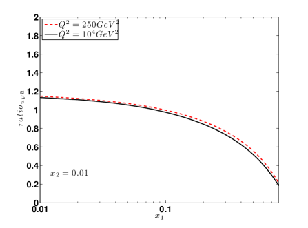
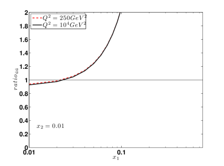
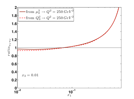
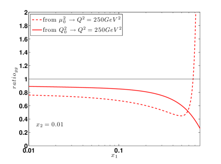
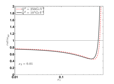
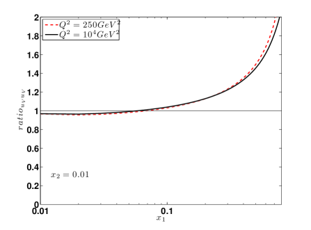
Figure 14: Left panel: The ratio Eq. (42) at different values of Q2superscript𝑄2Q^{2} as function of x1subscript𝑥1x_{1} at fixed x2=0.01subscript𝑥20.01x_{2}=0.01. Numerator and denominator are evolved by means of dPDF evolution and single parton evolution, respectively. The starting point is the low momentum scale μ02superscriptsubscript𝜇02\mu_{0}^{2}. Right panel: The same ratio for the valence-valence components within the same kinematical and dynamical conditions.
Refer to caption
Refer to caption
Figure 15: As in Fig. 14 for the ratio involving valence - sea (left panel) or sea - sea correlations (right panel). Notations as in Fig. 14.
Refer to caption
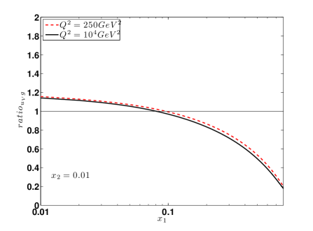
Figure 16: As in previous Figures for the ratio involving valence - gluon correlations. Notations as in Fig. 14.

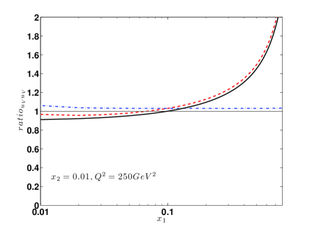
Results of the ratio Eq. (43) for the flavor combinations gg𝑔𝑔gg, uVuVsubscript𝑢𝑉subscript𝑢𝑉u_{V}u_{V}, uVu¯subscript𝑢𝑉¯𝑢u_{V}\bar{u}, u¯u¯¯𝑢¯𝑢\bar{u}\bar{u}, uVgsubscript𝑢𝑉𝑔u_{V}g are shown in Figs. 1416.

All the ratios have two common qualitative features:

  • i)

    results at Q2superscript𝑄2Q^{2} = 250 GeV2 do not really differ from those at Q2=104superscript𝑄2superscript104Q^{2}=10^{4} GeV2; the role of correlations does not depend therefore on the different high momentum scale which is chosen;

  • ii)

    in all flavor combinations, when at least one of the momentum fractions of the two partons is in the valence region, correlations are strong and the error which is done in approximating a dPDF with a product of sPDFs is huge.

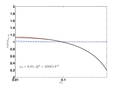
When both the momentum fractions of the partons are small, the situation is more involved. In the valence-valence sector, one finds negligible correlations and the ratio is basically 1 (cf. Fig. 14, right panel). This fact, in the Non-Singlet (NS) sector, had been already found and discussed in Ref. [14]. In all other cases, where singlet evolution is playing a role, even at values of x1,x2subscript𝑥1subscript𝑥2x_{1},x_{2} as low as 102superscript10210^{-2}, correlations are found to produce sizable deviations of the ratios from 1. The maximum effect is found in the gluon-gluon case (cf. Fig. 14, left panel), when it reaches 20 %percent\%. One should realize that, if two-parton correlations were present at the LHC scale, one could access through DPS studies novel information on the proton structure. Our evolved model results show that if one were able to measure dPDFs at a 20 %percent\% accuracy, a specific dynamical information would be reachable. The different behavior of the valence-valence sector from the others, as well as the fact that the gluon-gluon sector experiences the biggets effect, are interesting features of our results and deserve to be understood through a further investigation. This is carried on in the next section.

5.2 Perturbative versus Non-Perturbative Two-Parton Correlations

In this subsection we will find that the results described in the previous one can be understood by disentangling perturbative and non-perturbative effects.

To this aim, let us consider again the ratio Eq. (43)

ratioab=subscriptratio𝑎𝑏absent\displaystyle{\rm ratio}_{ab}= (45)
=Fab(x1,x2=0.01,k=0,Q2)+aba(x1,Q2)b(x2=0.01,Q2)+ab.\displaystyle={F_{ab}(x_{1},x_{2}=0.01,k_{\perp}=0,Q^{2})+a\to b\over a(x_{1},Q^{2})\cdot b(x_{2}=0.01,Q^{2})+a\to b}\,.

In the previous subsection 5.1, results are obtained evolving the numerator from μ02superscriptsubscript𝜇02\mu_{0}^{2} to Q2superscript𝑄2Q^{2}, considering at the lowest scale the dPDFs predicted by our LF-model. The denominator is obtained evolving to Q2superscript𝑄2Q^{2} the analogous sPDFs of the same LF-model.

A first consideration is in order: if the denominator, given by the product of single PDFs, had been evolved by means of dPDF-evolution criteria, we would have obtained a simplified approximation of the dPDFs at Q2superscript𝑄2Q^{2}, including perturbative correlations only.

Let us define the following quantity

Fab(x1,x2=0.01,k=0,Q2)|Perturbative=\displaystyle\left.F_{ab}(x_{1},x_{2}=0.01,k_{\perp}=0,Q^{2})\right|^{Perturbative}=
[a(x1,Q2)b(x2=0.01,Q2)]dPDFevolution.superscriptdelimited-[]𝑎subscript𝑥1superscript𝑄2𝑏subscript𝑥20.01superscript𝑄2𝑑𝑃𝐷𝐹𝑒𝑣𝑜𝑙𝑢𝑡𝑖𝑜𝑛\displaystyle\left[a(x_{1},Q^{2})\cdot b(x_{2}=0.01,Q^{2})\right]^{dPDF\,evolution}\,. (46)

In fact, Fab(x1,x2=0.01,k=0,Q2)|Perturbative\left.F_{ab}(x_{1},x_{2}=0.01,k_{\perp}=0,Q^{2})\right|^{Perturbative} contains those correlations which come from dPDF perturbative evolution only.

At this point, we could consider three different ratios:

  • i)

    the ratioab, Eq. (45);

  • ii)

    the ratioPerturbativeabsuperscriptsubscriptabsent𝑎𝑏𝑃𝑒𝑟𝑡𝑢𝑟𝑏𝑎𝑡𝑖𝑣𝑒{}_{ab}^{Perturbative}:

    ratioabPerturbative=superscriptsubscriptratio𝑎𝑏𝑃𝑒𝑟𝑡𝑢𝑟𝑏𝑎𝑡𝑖𝑣𝑒absent\displaystyle{\rm ratio}_{ab}^{Perturbative}=
    =\displaystyle= Fab(x1,x2=0.01,k=0,Q2)|Perturbative+aba(x1,Q2)b(x2=0.01,Q2)+ab,\displaystyle{\left.F_{ab}(x_{1},x_{2}=0.01,k_{\perp}=0,Q^{2})\right|^{Perturbative}+a\to b\over a(x_{1},Q^{2})\cdot b(x_{2}=0.01,Q^{2})+a\to b}\,,

    which contains perturbative correlations only; in fact it would be strictly 1 if the dPDF-evolution did not include double-parton correlations (see the definition Eq. (46));

  • iii)

    the ratioNonPerturbativeabsuperscriptsubscriptabsent𝑎𝑏𝑁𝑜𝑛𝑃𝑒𝑟𝑡𝑢𝑟𝑏𝑎𝑡𝑖𝑣𝑒{}_{ab}^{Non-Perturbative}

    ratioabNonPerturbative=superscriptsubscriptratio𝑎𝑏𝑁𝑜𝑛𝑃𝑒𝑟𝑡𝑢𝑟𝑏𝑎𝑡𝑖𝑣𝑒absent\displaystyle{\rm ratio}_{ab}^{Non-Perturbative}=
    =\displaystyle= Fab(x1,x2=0.01,k=0,Q2)+abFab(x1,x2=0.01,k=0,Q2)|Perturbative+ab,\displaystyle{F_{ab}(x_{1},x_{2}=0.01,k_{\perp}=0,Q^{2})+a\to b\over\left.F_{ab}(x_{1},x_{2}=0.01,k_{\perp}=0,Q^{2})\right|^{Perturbative}+a\to b}\,,

    which would be strictly 1 if only perturbative correlations were included in the numerator.
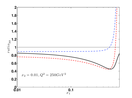
Refer to caption
Refer to caption
Figure 17: Left panel: The ratios (45) (dashed lines), (LABEL:eq:ratioabPerturbative) (dot-dashed lines) and (LABEL:eq:ratioabNonPerturbative) (continuous lines) specified for (ab)=(gg)𝑎𝑏𝑔𝑔(ab)=(gg) and at Q2=250superscript𝑄2250Q^{2}=250 GeV2 as function of x1subscript𝑥1x_{1} at fixed x2=0.01subscript𝑥20.01x_{2}=0.01. Right panel: The same ratios for the valence-valence components (ab)=(uVuV)𝑎𝑏subscript𝑢𝑉subscript𝑢𝑉(ab)=(u_{V}u_{V}) within the same kinematical and dynamical conditions.

The three ratios are very useful to disentangle the effects of perturbative versus non-perturbative double-parton correlations; of course the ratios (43) or (45) are the most complete, including both kind of correlations in a consistent way.

In Figs. 17, 18 and 19, the results for the three ratios are compared at the scale Q2=250superscript𝑄2250Q^{2}=250 GeV2, at x2=0.01subscript𝑥20.01x_{2}=0.01, as functions of x1subscript𝑥1x_{1}.

The ratiogg, shown in Fig. 17 (left panel), is particularly emblematic. The full ratiogg of Eq. (45) (dashed line), clearly influenced by both perturbative (dot-dashed line) and non-perturbative (continuous line) effects, is compared with those where perturbative and non-perturbative correlations are disentangled, contributing to the behavior of gluongluon𝑔𝑙𝑢𝑜𝑛𝑔𝑙𝑢𝑜𝑛gluon-gluon dPDFs at low values of x1subscript𝑥1x_{1} and x2subscript𝑥2x_{2}. The same comments hold for dPDFs corresponding to the other partons. An interesting feature of these results, clearly read in Figs. 17, 18 and 19, is that in few cases the perturbative and non-perturbative components tend to cancel (in the case of ValenceValence𝑉𝑎𝑙𝑒𝑛𝑐𝑒𝑉𝑎𝑙𝑒𝑛𝑐𝑒Valence-Valence illustrated in Fig. 17 (right panel), or u¯u¯¯𝑢¯𝑢\bar{u}-\bar{u}, as it borns out from Fig. 18 (right panel)). In the case of the gluon-gluon sector, the effect tends instead to sum coherently: this explains the persistence of correlations in this sector, even at high Q2superscript𝑄2Q^{2} and low x𝑥x, observed in the previous subsection.

In closing this Section, we conclude that correlations in dPDFs, for some flavor combinations, are present also at low x1subscript𝑥1x_{1} and x2subscript𝑥2x_{2}, even at the large energy scale of LHC experiments. This arises because perturbative and non-perturbative effects sum coherently. These conclusions are not artifacts of the specific LF model used. They hold qualitatively also in ratios obtained starting the evolution from Q02=1superscriptsubscript𝑄021Q_{0}^{2}=1 GeV2 >>μo2much-greater-thanabsentsuperscriptsubscript𝜇𝑜2>>\mu_{o}^{2}, using as non-perturbative input the semi-factorized model of Section IV. In order to illustrate this important point, two more plots are included (Fig. (20)). In the first one, the valence-valence ratio is shown, in the other the gluon-gluon one. These examples are illustrative, indeed, of two specific aspects: i) the valence-valence ratios should not depend on the starting point because they converge at the same values at the common hadronic scale μ02superscriptsubscript𝜇02\mu_{0}^{2}. The small differences which appear in the figures are therefore a clear estimate of the errors introduced by our numerical evolution and one can appreciate the precision of our approach; ii) the second figure, showing the gluon-gluon ratio, is included because the glue is the dominant component at low-x𝑥x and it contributes in a negligible way to the valence region. The correlations induced at low-x𝑥x still contain a specific sign of the correlations introduced in the valence sector and this is due to the presence of the valence component in the quark-singlet sector in the evolution procedure. The strength of the correlation seems to become smaller but they are still sizable.
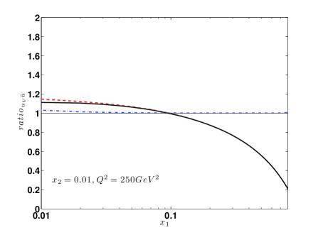
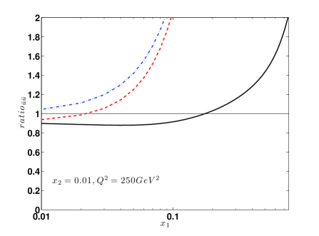
Refer to caption
Refer to caption
Figure 18: As in Fig. 17 for the ratio involving valence - sea (left panel) or sea - sea correlations (right panel). Notations as in Fig. 17.
Refer to caption
Figure 19: As in Figs. 18 and 19, for the ratio involving valence - gluon correlations. Notations as in Fig. 17.
Refer to caption
Refer to caption
Figure 20: Left panel: The ratio ratiouVuV𝑟𝑎𝑡𝑖subscript𝑜subscript𝑢𝑉subscript𝑢𝑉ratio_{u_{V}u_{V}} at Q2=250𝑄2250Q2=250 Gev2 as function of x1subscript𝑥1x_{1} at fixed x2=0.01subscript𝑥20.01x_{2}=0.01. Numerator and denom- inator are evolved by means of dPDF evolution and single parton evolution, respectively. The starting points differ for the two curves: the low momentum scale μ02superscriptsubscript𝜇02\mu_{0}^{2} (continuous) and the larger Q02subscriptsuperscript𝑄20Q^{2}_{0} (dashed) . The differences are artifacts due to numerical uncertainties. Right panel: the same of the left panel but for the ratiogg𝑟𝑎𝑡𝑖subscript𝑜𝑔𝑔ratio_{gg}.

6 Conclusions

Double Parton Scattering (DPS) represents a background in several channels for the search of new Physics at the LHC. Its correct description depends on our ability of modelling double parton distribution functions (dPDFs). The knowledge of these quantities would represent also a novel tool for the study of the three-dimensional nucleon structure, complementary to possibilities offered by electromagnetic interactions, in the framework of Generalized Parton Distribution functions. In this paper we have analyzed dPDFs, using Poincaré covariant predictions obtained, at a low energy scale, within a Light-Front model proposed by us in a recent paper, evolved using QCD evolution to experimentally relevant scales. We checked to what extent factorized expressions of dPDFs, in terms of products or convolutions of one-body densities, can be used, neglecting, at least in part, two-parton correlations. Our tests were performed using our model predictions starting from a scale where only quark degrees of freedom are relevant, or from higher scales, modeling sea quark and gluon contributions. Our model study demonstrates that factorization procedures strongly fail in reproducing the calculated dPDFs in the valence region, where measurements of DPS could really allow to access two-parton correlations. Besides, a gaussian behavior for the transverse distance in coordinate or momentum space seems rather arbitrary. Anyway, to have contact with measurable processes at existing facilities, everything has to be pushed to very low values of the longitudinal momenta of the interacting partons. This study has been carried on systematically and represents the most interesting part of our investigations. Correlations between pairs of partons of different kind have been considered, finding that, in some cases, their effect tends to be washed out at low-x𝑥x, as it happens for the valence, flavor non-singlet distributions, while they can affect other distributions in a sizable way, as in the gluon sector, when they can be as large as 20 %percent\%. We have shown that this different behavior can be understood in terms of a delicate interference of non-perturbative correlations, generated by the dynamics of the model, and perturbative ones, generated by the model independent evolution procedure. Our analysis shows that at LHC two-parton correlations can be relevant in DPS, opening a possibility to observe them for the first time. Our model dPDFs have now to be used to predict cross sections in specific channels where DPS is known to give an important contribution, such as, for example, the production of two W𝑊W bosons with the same sign. Our research is now addressing this final goal.

7 Acknowledgements

This work was supported in part by the Mineco under contract FPA2013-47443-C2-1-P, by GVA-PROMETEOII/2014/066 and SEV-2014-0398. S.S. thanks the Department of Theoretical Physics of the University of Valencia for warm hospitality and support. M.T. and V.V. thank the INFN, sezione di Perugia and the Department of Physics and Geology of the University of Perugia for warm hospitality and support. Several discussions with F.A. Ceccopieri are gratefully acknowledged.

Appendix A Appendix: Perturbative evolution of dPDFs in Mellin space

Following Diehl and Kasemets [44] one has to admit that “a consistent formulation of factorization for double parton scattering does not yet exist, so that it remains unclear how dPDFs should best be defined (and how they evolve)”. However some phenomenological aspects of QCD-evolution are known since long time (e.g Refs. [45, 46]) and have been recently retaken [47, 48, 49] developing numerical codes able to solve the evolution equations. In addition also theoretical progresses have been reported (for example the demonstration that the exchange of Glauber gluons cancels for the considered observable, a step forward in the proof of QCD factorization for DPS [50]).

In the following we develop a systematic numerical approach to the evolution of dPDFs, in Mellin space instead of coordinate space, restricting ourselves to the, so called, homogenous equation, a restriction we share with numerical solutions in coordinate space as applied in several contributions by Diehl and other coauthors (see Ref. [51] and reference therein).

If we assume equal renormalization scales Q1subscript𝑄1Q_{1} and Q2subscript𝑄2Q_{2} for the two partons (i.e. Q1=Q2=Qsubscript𝑄1subscript𝑄2𝑄Q_{1}=Q_{2}=Q), the LO evolution equation for the unpolarized double parton distributions Fj1j2(x1,x2;Q2)subscript𝐹subscript𝑗1subscript𝑗2subscript𝑥1subscript𝑥2superscript𝑄2F_{j_{1}j_{2}}(x_{1},x_{2};Q^{2}) then reads (see Ref. [52])

dFj1j2(x1,x2;Q2)dlogQ2|LO=αs(Q2)|LO4π×\displaystyle\left.{dF_{j_{1}j_{2}}(x_{1},x_{2};Q^{2})\over d\log Q^{2}}\right|_{\rm LO}={\left.\alpha_{s}(Q^{2})\right|_{\rm LO}\over 4\pi}\times
×[j1x11x2dy1y1Fj1j2(y1,x2;Q2)Pj1j1(x1y1)+\displaystyle\times\left[\sum_{j_{1}^{\prime}}\int_{x_{1}}^{1-x_{2}}{dy_{1}\over y_{1}}F_{j_{1}^{\prime}j_{2}}(y_{1},x_{2};Q^{2})P_{j_{1}^{\prime}\to j_{1}}\left({x_{1}\over y_{1}}\right)+\right.
+j2x21x1dy2y2Fj1j2(x1,y2;Q2)Pj2j2(x2y2)+limit-fromsubscriptsuperscriptsubscript𝑗2superscriptsubscriptsubscript𝑥21subscript𝑥1𝑑subscript𝑦2subscript𝑦2subscript𝐹subscript𝑗1superscriptsubscript𝑗2subscript𝑥1subscript𝑦2superscript𝑄2subscript𝑃superscriptsubscript𝑗2subscript𝑗2subscript𝑥2subscript𝑦2\displaystyle+\phantom{[[}\left.\sum_{j_{2}^{\prime}}\int_{x_{2}}^{1-x_{1}}{dy_{2}\over y_{2}}F_{j_{1}j_{2}^{\prime}}(x_{1},y_{2};Q^{2})P_{j_{2}^{\prime}\to j_{2}}\left({x_{2}\over y_{2}}\right)+\right.
+jFj(x1+x2;Q2)1x1+x2Pjj1j2(x1x1+x2)]\displaystyle+\left.\sum_{j^{\prime}}F_{j^{\prime}}(x_{1}+x_{2};Q^{2}){1\over x_{1}+x_{2}}P_{j^{\prime}\to j_{1}j_{2}}\left(x_{1}\over x_{1}+x_{2}\right)\right]
(49)

The convolution integrals appearing in Eq. (49) have the same structure of the integrals appearing in the evolution of the single parton distributions, namely the renormalization group equation (RGE). In order to solve evolution equations, one can perform a Mellin𝑀𝑒𝑙𝑙𝑖𝑛Mellin-transformation of Eqs. (49), in particular for the first two terms

dMj1j2n1n2(Q2)dlogQ2|LO=αs(Q2)|LO4π×\displaystyle\left.{dM_{j_{1}j_{2}}^{n_{1}n_{2}}(Q^{2})\over d\log Q^{2}}\right|_{\rm LO}={\left.\alpha_{s}(Q^{2})\right|_{\rm LO}\over 4\pi}\times
×[iPij1(0)(n1)Mij2n1n2(Q2)+\displaystyle\times\left[\sum_{i}P^{(0)}_{ij_{1}}(n_{1})M_{ij_{2}}^{n_{1}n_{2}}(Q^{2})+\right.
+kPkj2(0)(n2)Mj1kn1n2(Q2)]+\displaystyle\left.\phantom{[[}+\sum_{k}P^{(0)}_{kj_{2}}(n_{2})M_{j_{1}k}^{n_{1}n_{2}}(Q^{2})\right]+
+inhomogeneousterm,inhomogeneousterm\displaystyle\left.\phantom{[]}+{\rm inhomogeneous\,term}\right.\,, (50)

where

Mj1j2n1n2(Q2)superscriptsubscript𝑀subscript𝑗1subscript𝑗2subscript𝑛1subscript𝑛2superscript𝑄2\displaystyle M_{j_{1}j_{2}}^{n_{1}n_{2}}(Q^{2}) =\displaystyle= 01dx101dx2θ(1x1x2)\displaystyle\int_{0}^{1}dx_{1}\int_{0}^{1}dx_{2}\,\,\theta(1-x_{1}-x_{2})\,\cdot (51)
x1n11x2n21Fj1j2(x1,x2;Q2)absentsuperscriptsubscript𝑥1subscript𝑛11superscriptsubscript𝑥2subscript𝑛21subscript𝐹subscript𝑗1subscript𝑗2subscript𝑥1subscript𝑥2superscript𝑄2\displaystyle\phantom{}\cdot x_{1}^{n_{1}-1}x_{2}^{n_{2}-1}\,F_{j_{1}j_{2}}(x_{1},x_{2};Q^{2})
Pij(0)(n)subscriptsuperscript𝑃0𝑖𝑗𝑛\displaystyle P^{(0)}_{ij}(n) =\displaystyle= 01𝑑xxn1Pij(0)(x)superscriptsubscript01differential-d𝑥superscript𝑥𝑛1subscriptsuperscript𝑃0𝑖𝑗𝑥\displaystyle\int_{0}^{1}dx\,x^{n-1}\,P^{(0)}_{ij}(x) (52)

and the θ(1x1x2)𝜃1subscript𝑥1subscript𝑥2\theta(1-x_{1}-x_{2}) appearing in the definition of the moments Eq. (51) is a direct consequence of the limit of integration in Eq. (49) and the momentum conservation. Pijsubscript𝑃𝑖𝑗P_{ij} are the evolution kernels or splitting functions. They are calculated perturbatively as a series expansion in as(Q2)=αs(Q2)/(4π)subscript𝑎𝑠superscript𝑄2subscript𝛼𝑠superscript𝑄24𝜋a_{s}(Q^{2})=\alpha_{s}(Q^{2})/(4\pi):

Pij(xy,as(Q2))=m=0asm+1(Q2)Pij(m)(xy),subscript𝑃𝑖𝑗𝑥𝑦subscript𝑎𝑠superscript𝑄2superscriptsubscript𝑚0superscriptsubscript𝑎𝑠𝑚1superscript𝑄2superscriptsubscript𝑃𝑖𝑗𝑚𝑥𝑦P_{ij}\left({x\over y},a_{s}(Q^{2})\right)=\sum_{m=0}^{\infty}a_{s}^{m+1}(Q^{2})\,P_{ij}^{(m)}\left({x\over y}\right)\,, (53)

and m=0𝑚0m=0 indicates the Leading-Order contribution.

(Expressions for Pij(0)subscriptsuperscript𝑃0𝑖𝑗P^{(0)}_{ij} in the context of dPDFs can be found (e.g.) in Appendix A of Ref. [44]).

A.1 dPDF (flavor) decomposition and evolution

In order to solve Eqs. (50) one has to combine the flavor indices in a way consistent with evolution, in particular one has to identify combinations evolving as Singlet and Non-Singlet. The combinations depend on the order of the evolution. At LO and NLO a useful transformation is the following

ΣΣ\displaystyle\Sigma =\displaystyle= iqi+,Vi=qi,subscript𝑖superscriptsubscript𝑞𝑖subscript𝑉𝑖superscriptsubscript𝑞𝑖\displaystyle\sum_{i}q_{i}^{+},\;\;\;\;\;\;\;\;\;\;\,V_{i}=q_{i}^{-},
T3subscript𝑇3\displaystyle T_{3} =\displaystyle= u+d+,T8=u++d+2s+,superscript𝑢superscript𝑑subscript𝑇8superscript𝑢superscript𝑑2superscript𝑠\displaystyle u^{+}-d^{+},\;\;\;\;\;\;\;T_{8}=u^{+}+d^{+}-2s^{+}\,, (54)
withwith\displaystyle{\rm with}
qi±superscriptsubscript𝑞𝑖plus-or-minus\displaystyle q_{i}^{\pm} =\displaystyle= qi±q¯i;plus-or-minussubscript𝑞𝑖subscript¯𝑞𝑖\displaystyle q_{i}\pm\bar{q}_{i}\,;

and similar combination if one includes heavier quarks (e.g. Ref. [53] section 4.3.3). For the up and down quarks, Visubscript𝑉𝑖V_{i} corresponds to the valence contributions VuuVsubscript𝑉𝑢subscript𝑢𝑉V_{u}\equiv u_{V}, VddVsubscript𝑉𝑑subscript𝑑𝑉V_{d}\equiv d_{V}. After performing the evolution, the individual quark and antiquark distributions can be recovered using

u¯¯𝑢\displaystyle\bar{u} =\displaystyle= 14(23Σ+13T8+T3)12uV;1423Σ13subscript𝑇8subscript𝑇312subscript𝑢𝑉\displaystyle{1\over 4}\left({2\over 3}\Sigma+{1\over 3}T_{8}+T_{3}\right)-{1\over 2}u_{V};
d¯¯𝑑\displaystyle\bar{d} =\displaystyle= 14(23Σ+13T8T3)12dV.1423Σ13subscript𝑇8subscript𝑇312subscript𝑑𝑉\displaystyle{1\over 4}\left({2\over 3}\Sigma+{1\over 3}T_{8}-T_{3}\right)-{1\over 2}d_{V}.
s+s¯𝑠¯𝑠\displaystyle s+\bar{s} =\displaystyle= 13(ΣT8);13Σsubscript𝑇8\displaystyle{1\over 3}\left(\Sigma-T_{8}\right); (55)

Specifically, in the case of dPDFs Fijsubscript𝐹𝑖𝑗F_{ij}, the same argument holds for indices i,j𝑖𝑗i,j combined in such a way to produce T3subscript𝑇3T_{3}, T8subscript𝑇8T_{8} and Visubscript𝑉𝑖V_{i} structures. Consequently, in addition to FuVuVsubscript𝐹subscript𝑢𝑉subscript𝑢𝑉F_{u_{V}u_{V}}, FdVdVsubscript𝐹subscript𝑑𝑉subscript𝑑𝑉F_{d_{V}d_{V}} and FuVdVsubscript𝐹subscript𝑢𝑉subscript𝑑𝑉F_{u_{V}d_{V}}, FdVuVsubscript𝐹subscript𝑑𝑉subscript𝑢𝑉F_{d_{V}u_{V}}, also combinations like

FT3T3,FT3T8,FuVT3,FdVT3,FuVT8,FdVT8,subscript𝐹subscript𝑇3subscript𝑇3subscript𝐹subscript𝑇3subscript𝑇8subscript𝐹subscript𝑢𝑉subscript𝑇3subscript𝐹subscript𝑑𝑉subscript𝑇3subscript𝐹subscript𝑢𝑉subscript𝑇8subscript𝐹subscript𝑑𝑉subscript𝑇8\displaystyle F_{T_{3}T_{3}},\,\,F_{T_{3}T_{8}},\,\,F_{u_{V}T_{3}},\,\,F_{d_{V}T_{3}},\,\,F_{u_{V}T_{8}},\,\,F_{d_{V}T_{8}}, (56)

will evolve following the simple Non-Singlet rules.

Just to give an example, we will discuss, in the next Section, the evolution of the dPDF

FVuT3subscript𝐹subscript𝑉𝑢subscript𝑇3\displaystyle F_{V_{u}T_{3}} \displaystyle\equiv FuV(u+u¯dd¯)=subscript𝐹subscript𝑢𝑉𝑢¯𝑢𝑑¯𝑑absent\displaystyle F_{u_{V}(u+\bar{u}-d-\bar{d})}= (57)
=\displaystyle= FuVu+FuVu¯FuVdFuVd¯=subscript𝐹subscript𝑢𝑉𝑢subscript𝐹subscript𝑢𝑉¯𝑢subscript𝐹subscript𝑢𝑉𝑑subscript𝐹subscript𝑢𝑉¯𝑑absent\displaystyle F_{u_{V}u}+F_{u_{V}\bar{u}}-F_{u_{V}d}-F_{u_{V}\bar{d}}=
=\displaystyle= FuVuV+2FuVu¯FuVdV2FuVd¯.subscript𝐹subscript𝑢𝑉subscript𝑢𝑉2subscript𝐹subscript𝑢𝑉¯𝑢subscript𝐹subscript𝑢𝑉subscript𝑑𝑉2subscript𝐹subscript𝑢𝑉¯𝑑\displaystyle F_{u_{V}u_{V}}+2F_{u_{V}\bar{u}}-F_{u_{V}d_{V}}-2F_{u_{V}\bar{d}}\,.

Neglecting the inhomogeneous term, the solution of Eq. (50), for the Mellin moments of combination Eq. (57) is:

MVuT3n1n2(Q2)=(asas0)Pqq(0)(n1)+Pqq(0)(n2)β0MVuT3n1n2(Q02)superscriptsubscript𝑀subscript𝑉𝑢subscript𝑇3subscript𝑛1subscript𝑛2superscript𝑄2superscriptsubscript𝑎𝑠subscript𝑎𝑠0subscriptsuperscript𝑃0𝑞𝑞subscript𝑛1subscriptsuperscript𝑃0𝑞𝑞subscript𝑛2subscript𝛽0superscriptsubscript𝑀subscript𝑉𝑢subscript𝑇3subscript𝑛1subscript𝑛2superscriptsubscript𝑄02\displaystyle M_{V_{u}T_{3}}^{n_{1}n_{2}}(Q^{2})=\left({a_{s}\over a_{s0}}\right)^{-{P^{(0)}_{qq}(n_{1})+P^{(0)}_{qq}(n_{2})\over\beta_{0}}}\cdot M_{V_{u}T_{3}}^{n_{1}n_{2}}(Q_{0}^{2})\,

(compare also the definition Eq. (51)).

The Mellin𝑀𝑒𝑙𝑙𝑖𝑛Mellin-inversion completes the solution in x𝑥x-space:

FVuT3(x1,x2,Q2)=subscript𝐹subscript𝑉𝑢subscript𝑇3subscript𝑥1subscript𝑥2superscript𝑄2absent\displaystyle F_{V_{u}T_{3}}(x_{1},x_{2},Q^{2})=
=12πi𝒞𝑑n112πi𝒞𝑑n2x1(1n1)x2(1n2)MVuT3n1n2(Q2).absent12𝜋𝑖subscriptcontour-integral𝒞differential-dsubscript𝑛112𝜋𝑖subscriptcontour-integral𝒞differential-dsubscript𝑛2superscriptsubscript𝑥11subscript𝑛1superscriptsubscript𝑥21subscript𝑛2superscriptsubscript𝑀subscript𝑉𝑢subscript𝑇3subscript𝑛1subscript𝑛2superscript𝑄2\displaystyle={1\over 2\pi i}\oint_{\cal C}dn_{1}\,{1\over 2\pi i}\oint_{\cal C}dn_{2}\,x_{1}^{(1-n_{1})}\,x_{2}^{(1-n_{2})}\,M_{V_{u}T_{3}}^{n_{1}n_{2}}(Q^{2})\,.
(59)

The procedure described for the example FVuT3subscript𝐹subscript𝑉𝑢subscript𝑇3F_{V_{u}T_{3}}, is valid for each Fijsubscript𝐹𝑖𝑗F_{ij} combination ((i,j)=Vi,T3,T8𝑖𝑗subscript𝑉𝑖subscript𝑇3subscript𝑇8(i,j)=V_{i}\,,T_{3}\,,T_{8}).

On the other hand, the double𝑑𝑜𝑢𝑏𝑙𝑒double-distributions containing gluons𝑔𝑙𝑢𝑜𝑛𝑠gluons and ΣΣ\Sigma evolve mixing the two and each index must be evolved in the appropriate way. For example:

(MVuΣn1n2(Q2)MVugn1n2(Q2))=(asas0)Pqq(0)(n1)β0×\displaystyle\left(\begin{array}[]{c}M_{V_{u}\Sigma}^{n_{1}n_{2}}(Q^{2})\\ \\ M_{V_{u}g}^{n_{1}n_{2}}(Q^{2})\\ \end{array}\right)=\left({a_{s}\over a_{s0}}\right)^{-{P^{(0)}_{qq}(n_{1})\over\beta_{0}}}\times (63)
×(Wqq0(n2)Wqg0(n2)Wgq0(n2)Wgg0(n2))(MVuΣn1n2(Q02)MVugn1n2(Q02)),absentsubscriptsuperscript𝑊0𝑞𝑞subscript𝑛2subscriptsuperscript𝑊0𝑞𝑔subscript𝑛2missing-subexpressionmissing-subexpressionsubscriptsuperscript𝑊0𝑔𝑞subscript𝑛2subscriptsuperscript𝑊0𝑔𝑔subscript𝑛2superscriptsubscript𝑀subscript𝑉𝑢Σsubscript𝑛1subscript𝑛2superscriptsubscript𝑄02missing-subexpressionsuperscriptsubscript𝑀subscript𝑉𝑢𝑔subscript𝑛1subscript𝑛2superscriptsubscript𝑄02\displaystyle\times\left(\begin{array}[]{cc}W^{0}_{qq}(n_{2})&W^{0}_{qg}(n_{2})\\ &\\ W^{0}_{gq}(n_{2})&W^{0}_{gg}(n_{2})\\ \end{array}\right)\cdot\left(\begin{array}[]{c}M_{V_{u}\Sigma}^{n_{1}n_{2}}(Q_{0}^{2})\\ \\ M_{V_{u}g}^{n_{1}n_{2}}(Q_{0}^{2})\\ \end{array}\right), (70)

a result valid also replacing the first index Vusubscript𝑉𝑢V_{u} with the other Non-Singlet components, namely T3subscript𝑇3T_{3} or T8subscript𝑇8T_{8}.

Last examples the SingletSinglet𝑆𝑖𝑛𝑔𝑙𝑒𝑡𝑆𝑖𝑛𝑔𝑙𝑒𝑡Singlet-Singlet components:

MΣΣn1n2(Q2)superscriptsubscript𝑀ΣΣsubscript𝑛1subscript𝑛2superscript𝑄2\displaystyle M_{\Sigma\Sigma}^{n_{1}n_{2}}(Q^{2}) =\displaystyle= Wqq0(n1)Wqq0(n2)MΣΣn1n2(Q02)+limit-fromsubscriptsuperscript𝑊0𝑞𝑞subscript𝑛1subscriptsuperscript𝑊0𝑞𝑞subscript𝑛2superscriptsubscript𝑀ΣΣsubscript𝑛1subscript𝑛2superscriptsubscript𝑄02\displaystyle W^{0}_{qq}(n_{1})W^{0}_{qq}(n_{2})M_{\Sigma\Sigma}^{n_{1}n_{2}}(Q_{0}^{2})+ (71)
+\displaystyle+ Wqg0(n1)Wqq0(n2)MgΣn1n2(Q02)+limit-fromsubscriptsuperscript𝑊0𝑞𝑔subscript𝑛1subscriptsuperscript𝑊0𝑞𝑞subscript𝑛2superscriptsubscript𝑀𝑔Σsubscript𝑛1subscript𝑛2superscriptsubscript𝑄02\displaystyle W^{0}_{qg}(n_{1})W^{0}_{qq}(n_{2})M_{g\Sigma}^{n_{1}n_{2}}(Q_{0}^{2})+
+\displaystyle+ Wqq0(n1)Wqg0(n2)MΣgn1n2(Q02)+limit-fromsubscriptsuperscript𝑊0𝑞𝑞subscript𝑛1subscriptsuperscript𝑊0𝑞𝑔subscript𝑛2superscriptsubscript𝑀Σ𝑔subscript𝑛1subscript𝑛2superscriptsubscript𝑄02\displaystyle W^{0}_{qq}(n_{1})W^{0}_{qg}(n_{2})M_{\Sigma g}^{n_{1}n_{2}}(Q_{0}^{2})+
+\displaystyle+ Wqg0(n1)Wqg0(n2)Mggn1n2(Q02);subscriptsuperscript𝑊0𝑞𝑔subscript𝑛1subscriptsuperscript𝑊0𝑞𝑔subscript𝑛2superscriptsubscript𝑀𝑔𝑔subscript𝑛1subscript𝑛2superscriptsubscript𝑄02\displaystyle W^{0}_{qg}(n_{1})W^{0}_{qg}(n_{2})M_{gg}^{n_{1}n_{2}}(Q_{0}^{2})\,;
Mggn1n2(Q2)superscriptsubscript𝑀𝑔𝑔subscript𝑛1subscript𝑛2superscript𝑄2\displaystyle M_{gg}^{n_{1}n_{2}}(Q^{2}) =\displaystyle= Wgg0(n1)Wgg0(n2)Mggn1n2(Q02)+limit-fromsubscriptsuperscript𝑊0𝑔𝑔subscript𝑛1subscriptsuperscript𝑊0𝑔𝑔subscript𝑛2superscriptsubscript𝑀𝑔𝑔subscript𝑛1subscript𝑛2superscriptsubscript𝑄02\displaystyle W^{0}_{gg}(n_{1})W^{0}_{gg}(n_{2})M_{gg}^{n_{1}n_{2}}(Q_{0}^{2})+ (72)
+\displaystyle+ Wgq0(n1)Wgg0(n2)MΣgn1n2(Q02)+limit-fromsubscriptsuperscript𝑊0𝑔𝑞subscript𝑛1subscriptsuperscript𝑊0𝑔𝑔subscript𝑛2superscriptsubscript𝑀Σ𝑔subscript𝑛1subscript𝑛2superscriptsubscript𝑄02\displaystyle W^{0}_{gq}(n_{1})W^{0}_{gg}(n_{2})M_{\Sigma g}^{n_{1}n_{2}}(Q_{0}^{2})+
+\displaystyle+ Wgg0(n1)Wgq0(n2)MgΣn1n2(Q02)+limit-fromsubscriptsuperscript𝑊0𝑔𝑔subscript𝑛1subscriptsuperscript𝑊0𝑔𝑞subscript𝑛2superscriptsubscript𝑀𝑔Σsubscript𝑛1subscript𝑛2superscriptsubscript𝑄02\displaystyle W^{0}_{gg}(n_{1})W^{0}_{gq}(n_{2})M_{g\Sigma}^{n_{1}n_{2}}(Q_{0}^{2})+
+\displaystyle+ Wgq0(n1)Wgq0(n2)MΣΣn1n2(Q02);subscriptsuperscript𝑊0𝑔𝑞subscript𝑛1subscriptsuperscript𝑊0𝑔𝑞subscript𝑛2superscriptsubscript𝑀ΣΣsubscript𝑛1subscript𝑛2superscriptsubscript𝑄02\displaystyle W^{0}_{gq}(n_{1})W^{0}_{gq}(n_{2})M_{\Sigma\Sigma}^{n_{1}n_{2}}(Q_{0}^{2})\,;
MΣgn1n2(Q2)superscriptsubscript𝑀Σ𝑔subscript𝑛1subscript𝑛2superscript𝑄2\displaystyle M_{\Sigma g}^{n_{1}n_{2}}(Q^{2}) =\displaystyle= Wqq0(n1)Wgg0(n2)MΣgn1n2(Q02)+limit-fromsubscriptsuperscript𝑊0𝑞𝑞subscript𝑛1subscriptsuperscript𝑊0𝑔𝑔subscript𝑛2superscriptsubscript𝑀Σ𝑔subscript𝑛1subscript𝑛2superscriptsubscript𝑄02\displaystyle W^{0}_{qq}(n_{1})W^{0}_{gg}(n_{2})M_{\Sigma g}^{n_{1}n_{2}}(Q_{0}^{2})+ (73)
+\displaystyle+ Wqg0(n1)Wgg0(n2)Mggn1n2(Q02)+limit-fromsubscriptsuperscript𝑊0𝑞𝑔subscript𝑛1subscriptsuperscript𝑊0𝑔𝑔subscript𝑛2superscriptsubscript𝑀𝑔𝑔subscript𝑛1subscript𝑛2superscriptsubscript𝑄02\displaystyle W^{0}_{qg}(n_{1})W^{0}_{gg}(n_{2})M_{gg}^{n_{1}n_{2}}(Q_{0}^{2})+
+\displaystyle+ Wqq0(n1)Wgq0(n2)MΣΣn1n2(Q02)+limit-fromsubscriptsuperscript𝑊0𝑞𝑞subscript𝑛1subscriptsuperscript𝑊0𝑔𝑞subscript𝑛2superscriptsubscript𝑀ΣΣsubscript𝑛1subscript𝑛2superscriptsubscript𝑄02\displaystyle W^{0}_{qq}(n_{1})W^{0}_{gq}(n_{2})M_{\Sigma\Sigma}^{n_{1}n_{2}}(Q_{0}^{2})+
+\displaystyle+ Wqg0(n1)Wqg0(n2)MgΣn1n2(Q02);subscriptsuperscript𝑊0𝑞𝑔subscript𝑛1subscriptsuperscript𝑊0𝑞𝑔subscript𝑛2superscriptsubscript𝑀𝑔Σsubscript𝑛1subscript𝑛2superscriptsubscript𝑄02\displaystyle W^{0}_{qg}(n_{1})W^{0}_{qg}(n_{2})M_{g\Sigma}^{n_{1}n_{2}}(Q_{0}^{2})\,;
MgΣn1n2(Q2)superscriptsubscript𝑀𝑔Σsubscript𝑛1subscript𝑛2superscript𝑄2\displaystyle M_{g\Sigma}^{n_{1}n_{2}}(Q^{2}) =\displaystyle= Wgq0(n1)Wqg0(n2)MΣgn1n2(Q02)+limit-fromsubscriptsuperscript𝑊0𝑔𝑞subscript𝑛1subscriptsuperscript𝑊0𝑞𝑔subscript𝑛2superscriptsubscript𝑀Σ𝑔subscript𝑛1subscript𝑛2superscriptsubscript𝑄02\displaystyle W^{0}_{gq}(n_{1})W^{0}_{qg}(n_{2})M_{\Sigma g}^{n_{1}n_{2}}(Q_{0}^{2})+ (74)
+\displaystyle+ Wgg0(n1)Wqg0(n2)Mggn1n2(Q02)+limit-fromsubscriptsuperscript𝑊0𝑔𝑔subscript𝑛1subscriptsuperscript𝑊0𝑞𝑔subscript𝑛2superscriptsubscript𝑀𝑔𝑔subscript𝑛1subscript𝑛2superscriptsubscript𝑄02\displaystyle W^{0}_{gg}(n_{1})W^{0}_{qg}(n_{2})M_{gg}^{n_{1}n_{2}}(Q_{0}^{2})+
+\displaystyle+ Wgq0(n1)Wqq0(n2)MΣΣn1n2(Q02)+limit-fromsubscriptsuperscript𝑊0𝑔𝑞subscript𝑛1subscriptsuperscript𝑊0𝑞𝑞subscript𝑛2superscriptsubscript𝑀ΣΣsubscript𝑛1subscript𝑛2superscriptsubscript𝑄02\displaystyle W^{0}_{gq}(n_{1})W^{0}_{qq}(n_{2})M_{\Sigma\Sigma}^{n_{1}n_{2}}(Q_{0}^{2})+
+\displaystyle+ Wgg0(n1)Wqq0(n2)MgΣn1n2(Q02).subscriptsuperscript𝑊0𝑔𝑔subscript𝑛1subscriptsuperscript𝑊0𝑞𝑞subscript𝑛2superscriptsubscript𝑀𝑔Σsubscript𝑛1subscript𝑛2superscriptsubscript𝑄02\displaystyle W^{0}_{gg}(n_{1})W^{0}_{qq}(n_{2})M_{g\Sigma}^{n_{1}n_{2}}(Q_{0}^{2})\,.

The Mellin𝑀𝑒𝑙𝑙𝑖𝑛Mellin-inversion Eq. (59), completes again the procedure.

A.2 Examples of Flavor decomposition

  • A.

    Flavor decomposition at the generic scale Q2superscript𝑄2Q^{2}

    Fuusubscript𝐹superscript𝑢superscript𝑢\displaystyle F_{u^{-}u^{-}} =\displaystyle= F(uu¯)(uu¯)FuVuV;subscript𝐹𝑢¯𝑢𝑢¯𝑢subscript𝐹subscript𝑢𝑉subscript𝑢𝑉\displaystyle F_{(u-\bar{u})(u-\bar{u})}\equiv F_{u_{V}u_{V}}\,; (75)
    Fu+u+subscript𝐹superscript𝑢superscript𝑢\displaystyle F_{u^{+}u^{+}} =\displaystyle= F(u+u¯)(u+u¯)=FuVuV+2[FuVu¯+Fu¯uV]+4Fu¯u¯=subscript𝐹𝑢¯𝑢𝑢¯𝑢subscript𝐹subscript𝑢𝑉subscript𝑢𝑉2delimited-[]subscript𝐹subscript𝑢𝑉¯𝑢subscript𝐹¯𝑢subscript𝑢𝑉4subscript𝐹¯𝑢¯𝑢absent\displaystyle F_{(u+\bar{u})(u+\bar{u})}=F_{u_{V}u_{V}}+2\left[F_{u_{V}\bar{u}}+F_{\bar{u}u_{V}}\right]+4F_{\bar{u}\bar{u}}= (76)
    =\displaystyle= 116[4FΣΣ+FT8T8+9FT3T3+\displaystyle{1\over 16}\left[4F_{\Sigma\Sigma}+F_{T_{8}T_{8}}+9F_{T_{3}T_{3}}+\right.
    +\displaystyle+ 2(FΣT8+FT8Σ)+3(FT8T3+FT3T8)+2subscript𝐹Σsubscript𝑇8subscript𝐹subscript𝑇8Σlimit-from3subscript𝐹subscript𝑇8subscript𝑇3subscript𝐹subscript𝑇3subscript𝑇8\displaystyle 2(F_{\Sigma T_{8}}+F_{T_{8}\Sigma})+3(F_{T_{8}T_{3}}+F_{T_{3}T_{8}})+
    +\displaystyle+ 6(FΣT3+FT3Σ)];\displaystyle\left.6(F_{\Sigma T_{3}}+F_{T_{3}\Sigma})\right]\,;

    and the inverse

    FΣΣsubscript𝐹ΣΣ\displaystyle F_{\Sigma\Sigma} =\displaystyle= Fu+u++Fd+d++Fs+s++subscript𝐹superscript𝑢superscript𝑢subscript𝐹superscript𝑑superscript𝑑limit-fromsubscript𝐹superscript𝑠superscript𝑠\displaystyle F_{u^{+}u^{+}}+F_{d^{+}d^{+}}+F_{s^{+}s^{+}}+ (78)
    +\displaystyle+ (Fu+d++Fd+u+)+(Fu+s++Fs+u+)+subscript𝐹superscript𝑢superscript𝑑subscript𝐹superscript𝑑superscript𝑢limit-fromsubscript𝐹superscript𝑢superscript𝑠subscript𝐹superscript𝑠superscript𝑢\displaystyle(F_{u^{+}d^{+}}+F_{d^{+}u^{+}})+(F_{u^{+}s^{+}}+F_{s^{+}u^{+}})+
    +\displaystyle+ (Fd+s++Fs+d+);subscript𝐹superscript𝑑superscript𝑠subscript𝐹superscript𝑠superscript𝑑\displaystyle(F_{d^{+}s^{+}}+F_{s^{+}d^{+}})\,;
    FT3T3subscript𝐹subscript𝑇3subscript𝑇3\displaystyle F_{T_{3}T_{3}} =\displaystyle= Fu+u++Fd+d++subscript𝐹superscript𝑢superscript𝑢limit-fromsubscript𝐹superscript𝑑superscript𝑑\displaystyle F_{u^{+}u^{+}}+F_{d^{+}d^{+}}+ (79)
    \displaystyle- (Fu+d++Fd+u+);subscript𝐹superscript𝑢superscript𝑑subscript𝐹superscript𝑑superscript𝑢\displaystyle(F_{u^{+}d^{+}}+F_{d^{+}u^{+}})\,;
    FΣT8+FT8Σsubscript𝐹Σsubscript𝑇8subscript𝐹subscript𝑇8Σ\displaystyle F_{\Sigma T_{8}}+F_{T_{8}\Sigma} =\displaystyle= 2Fu+u++2Fd+d+4Fs+s++2subscript𝐹superscript𝑢superscript𝑢2subscript𝐹superscript𝑑superscript𝑑limit-from4subscript𝐹superscript𝑠superscript𝑠\displaystyle 2F_{u^{+}u^{+}}+2F_{d^{+}d^{+}}-4F_{s^{+}s^{+}}+
    +\displaystyle+ 2(Fu+d++Fd+u+)+limit-from2subscript𝐹superscript𝑢superscript𝑑subscript𝐹superscript𝑑superscript𝑢\displaystyle 2(F_{u^{+}d^{+}}+F_{d^{+}u^{+}})+
    \displaystyle- (Fu+s++Fs+u+)+limit-fromsubscript𝐹superscript𝑢superscript𝑠subscript𝐹superscript𝑠superscript𝑢\displaystyle(F_{u^{+}s^{+}}+F_{s^{+}u^{+}})+
    \displaystyle- (Fd+s++Fs+d+);subscript𝐹superscript𝑑superscript𝑠subscript𝐹superscript𝑠superscript𝑑\displaystyle(F_{d^{+}s^{+}}+F_{s^{+}d^{+}})\,; (81)
    FΣT3+FT3Σsubscript𝐹Σsubscript𝑇3subscript𝐹subscript𝑇3Σ\displaystyle F_{\Sigma T_{3}}+F_{T_{3}\Sigma} =\displaystyle= 2Fu+u+2Fd+d++2subscript𝐹superscript𝑢superscript𝑢limit-from2subscript𝐹superscript𝑑superscript𝑑\displaystyle 2F_{u^{+}u^{+}}-2F_{d^{+}d^{+}}+
    \displaystyle- (Fu+s++Fs+u+)+limit-fromsubscript𝐹superscript𝑢superscript𝑠subscript𝐹superscript𝑠superscript𝑢\displaystyle(F_{u^{+}s^{+}}+F_{s^{+}u^{+}})+
    \displaystyle- (Fd+s++Fs+d+);subscript𝐹superscript𝑑superscript𝑠subscript𝐹superscript𝑠superscript𝑑\displaystyle(F_{d^{+}s^{+}}+F_{s^{+}d^{+}})\,; (83)
    FT3T8+FT8T3subscript𝐹subscript𝑇3subscript𝑇8subscript𝐹subscript𝑇8subscript𝑇3\displaystyle F_{T_{3}T_{8}}+F_{T_{8}T_{3}} =\displaystyle= 2Fu+u++2Fd+d++2subscript𝐹superscript𝑢superscript𝑢limit-from2subscript𝐹superscript𝑑superscript𝑑\displaystyle 2F_{u^{+}u^{+}}+2F_{d^{+}d^{+}}+
    \displaystyle- 2(Fu+s++Fs+u+)+limit-from2subscript𝐹superscript𝑢superscript𝑠subscript𝐹superscript𝑠superscript𝑢\displaystyle 2(F_{u^{+}s^{+}}+F_{s^{+}u^{+}})+
    +\displaystyle+ (Fd+s++Fs+d+);subscript𝐹superscript𝑑superscript𝑠subscript𝐹superscript𝑠superscript𝑑\displaystyle(F_{d^{+}s^{+}}+F_{s^{+}d^{+}})\,; (85)

    These relations are generally valid, not only at the specific Q02superscriptsubscript𝑄02Q_{0}^{2}.

  • B.

    Reduction at the μ02superscriptsubscript𝜇02\mu_{0}^{2} scale

    At the lowest scale one has:

    Fuusubscript𝐹superscript𝑢superscript𝑢\displaystyle F_{u^{-}u^{-}} =\displaystyle= F(uu¯)(uu¯)FuVuV=subscript𝐹𝑢¯𝑢𝑢¯𝑢subscript𝐹subscript𝑢𝑉subscript𝑢𝑉absent\displaystyle F_{(u-\bar{u})(u-\bar{u})}\equiv F_{u_{V}u_{V}}= (87)
    =\displaystyle= uVuV(x1,x2,μ02);subscript𝑢𝑉subscript𝑢𝑉subscript𝑥1subscript𝑥2superscriptsubscript𝜇02\displaystyle u_{V}u_{V}(x_{1},x_{2},\mu_{0}^{2})\,;
    Fu+u+subscript𝐹superscript𝑢superscript𝑢\displaystyle F_{u^{+}u^{+}} =\displaystyle= F(u+u¯)(u+u¯)=FuVuV+subscript𝐹𝑢¯𝑢𝑢¯𝑢limit-fromsubscript𝐹subscript𝑢𝑉subscript𝑢𝑉\displaystyle F_{(u+\bar{u})(u+\bar{u})}=F_{u_{V}u_{V}}+ (88)
    +\displaystyle+ 2[FuVu¯+Fu¯uV]+4Fu¯u¯=2delimited-[]subscript𝐹subscript𝑢𝑉¯𝑢subscript𝐹¯𝑢subscript𝑢𝑉4subscript𝐹¯𝑢¯𝑢absent\displaystyle 2\left[F_{u_{V}\bar{u}}+F_{\bar{u}u_{V}}\right]+4F_{\bar{u}\bar{u}}=
    =\displaystyle= uVuV(x1,x2,μ02);subscript𝑢𝑉subscript𝑢𝑉subscript𝑥1subscript𝑥2superscriptsubscript𝜇02\displaystyle u_{V}u_{V}(x_{1},x_{2},\mu_{0}^{2})\,;
    Fs+s+subscript𝐹superscript𝑠superscript𝑠\displaystyle F_{s^{+}s^{+}} =\displaystyle= 0;0\displaystyle 0\,; (89)
    Fggsubscript𝐹𝑔𝑔\displaystyle F_{gg} =\displaystyle= 0.0\displaystyle 0\,. (90)

    and the inverse

    FΣΣsubscript𝐹ΣΣ\displaystyle F_{\Sigma\Sigma} =\displaystyle= 3FuVuV;3subscript𝐹subscript𝑢𝑉subscript𝑢𝑉\displaystyle 3F_{u_{V}u_{V}}\,; (91)
    FT3T3subscript𝐹subscript𝑇3subscript𝑇3\displaystyle F_{T_{3}T_{3}} =\displaystyle= FuVuV;subscript𝐹subscript𝑢𝑉subscript𝑢𝑉\displaystyle-F_{u_{V}u_{V}}\,; (92)
    FT8T8subscript𝐹subscript𝑇8subscript𝑇8\displaystyle F_{T_{8}T_{8}} =\displaystyle= 3FuVuV;3subscript𝐹subscript𝑢𝑉subscript𝑢𝑉\displaystyle 3F_{u_{V}u_{V}}\,; (93)
    FΣT3+FT3Σsubscript𝐹Σsubscript𝑇3subscript𝐹subscript𝑇3Σ\displaystyle F_{\Sigma T_{3}}+F_{T_{3}\Sigma} =\displaystyle= 2FuVuV;2subscript𝐹subscript𝑢𝑉subscript𝑢𝑉\displaystyle 2F_{u_{V}u_{V}}\,; (94)
    FΣT8+FT8Σsubscript𝐹Σsubscript𝑇8subscript𝐹subscript𝑇8Σ\displaystyle F_{\Sigma T_{8}}+F_{T_{8}\Sigma} =\displaystyle= 6FuVuV;6subscript𝐹subscript𝑢𝑉subscript𝑢𝑉\displaystyle 6F_{u_{V}u_{V}}\,; (95)
    FT3T8+FT8T3subscript𝐹subscript𝑇3subscript𝑇8subscript𝐹subscript𝑇8subscript𝑇3\displaystyle F_{T_{3}T_{8}}+F_{T_{8}T_{3}} =\displaystyle= 2FuVuV.2subscript𝐹subscript𝑢𝑉subscript𝑢𝑉\displaystyle 2F_{u_{V}u_{V}}\,. (96)

    These relations are valid when the contributions at μ02superscriptsubscript𝜇02\mu_{0}^{2} reduce to valence contributions only.

References

  • [1] N. Paver and D. Treleani, Nuovo Cim. A 70, 215 (1982).
  • [2] J. R. Gaunt and W. J. Stirling, JHEP 03, 005 (2010).
  • [3] M. Diehl, D. Ostermeier and A. Schafer, JHEP 03, 089 (2012).
  • [4] A. V. Manohar and W. J. Waalewijn, Phys. Rev. D 85, 114009 (2012).
  • [5] S. Bansal, P. Bartalini, B. Blok, D. Ciangottini, M. Diehl, F. M. Fionda, J. R. Gaunt, P. Gunnellini et al., arXiv:1410.6664 [hep-ph].
  • [6] A. Szczurek, arXiv:1504.06491 [hep-ph].
  • [7] G. Calucci and D. Treleani, Phys. Rev. D 60, 054023 (1999).
  • [8] M. Guidal, H. Moutarde and M. Vanderhaeghen, Rept. Prog. Phys.  76, 066202 (2013).
  • [9] R. Dupre, M. Guidal and M. Vanderhaeghen, arXiv:1606.07821 [hep-ph].
  • [10] E. Cattaruzza, A. Del Fabbro and D. Treleani, Phys. Rev. D 72, 034022 (2005).
  • [11] M. G. Echevarria, T. Kasemets, P. J. Mulders and C. Pisano, JHEP 04, 034 (2015).
  • [12] H. M. Chang, A. V. Manohar and W. J. Waalewijn, Phys. Rev. D 87, no. 3, 034009 (2013).
  • [13] M. Rinaldi, S. Scopetta and V. Vento, Phys. Rev. D 87, 114021 (2013).
  • [14] M. Rinaldi, S. Scopetta, M. Traini and V. Vento, JHEP 12, 028 (2014).
  • [15] W. Broniowski and E. Ruiz Arriola, Few Body Syst.  55, 381 (2014).
  • [16] W. Broniowski, E. Ruiz Arriola and K. Golec-Biernat, Few Body Syst.  57, no. 6, 405 (2016).
  • [17] T. Akesson et al. [Axial Field Spectrometer Collaboration], Z. Phys. C 34, 163 (1987).
  • [18] J. Alitti et al. [UA2 Collaboration], Phys. Lett. B 268, 145 (1991).
  • [19] F. Abe et al. [CDF Collaboration], Phys. Rev. D 56, 3811 (1997).
  • [20] V. M. Abazov et al. [D0 Collaboration], Phys. Rev. D 81, 052012 (2010).
  • [21] G. Aad et al. [ATLAS Collaboration], New J. Phys.  15, 033038 (2013).
  • [22] S. Chatrchyan et al. [CMS Collaboration], JHEP 03, 032 (2014).
  • [23] M. Rinaldi, S. Scopetta, M. Traini and V. Vento, Phys. Lett. B 752, 40 (2016).
  • [24] P. Faccioli, M. Traini and V. Vento, Nucl. Phys. A 656, 400 (1999).
  • [25] M. Ferraris, M. M. Giannini, M. Pizzo, E. Santopinto and L. Tiator, Phys. Lett. B 364, 231 (1995).
  • [26] B. Pasquini, M. Traini and S. Boffi, Phys. Rev. D 65, 074028 (2002).
  • [27] M. Traini, Phys. Lett. B 707, 523 (2012).
  • [28] M. Traini, Phys. Rev. D 89, no. 3, 034021 (2014).
  • [29] F. Cano, P. Faccioli and M. Traini, Phys. Rev. D 62, 094018 (2000).
  • [30] F. Cano, P. Faccioli, S. Scopetta and M. Traini, Phys. Rev. D 62, 054023 (2000).
  • [31] S. Boffi, B. Pasquini and M. Traini, Nucl. Phys. B 649, 243 (2003);
    S. Boffi, B. Pasquini and M. Traini, Nucl. Phys. B 680, 147 (2004);
    B. Pasquini, M. Traini and S. Boffi, Phys. Rev. D 71, 034022 (2005).
  • [32] B. Blok, Y. Dokshitser, L. Frankfurt and M. Strikman, Eur. Phys. J. C 72, 1963 (2012).
  • [33] B. Blok, Y. Dokshitzer, L. Frankfurt and M. Strikman, Eur. Phys. J. C 74, 2926 (2014).
  • [34] S. J. Brodsky, H. C. Pauli and S. S. Pinsky, Phys. Rept.  301, 299 (1998).
  • [35] H. J. Melosh, Phys. Rev. D 9, 1095 (1974).
  • [36] B. Bakamjian and L. H. Thomas, Phys. Rev.  92, 1300 (1953).
  • [37] M. Traini, A. Mair, A. Zambarda and V. Vento, Nucl. Phys. A 614, 472 (1997).
  • [38] M. Diehl, T. Kasemets and S. Keane, JHEP 05, 118 (2014).
  • [39] A. D. Martin, W. J. Stirling, R. S. Thorne and G. Watt, Eur. Phys. J. C 63, 189 (2009).
  • [40] M. Diehl, Phys. Rept.  388, 41 (2003).
  • [41] J. R. Gaunt, R. Maciula and A. Szczurek, Phys. Rev. D 90, no. 5, 054017 (2014).
  • [42] B. Pasquini and S. Boffi, Phys. Rev. D 73, 094001 (2006).
  • [43] V. L. Korotkikh and A. M. Snigirev, Phys. Lett. B 594, 171 (2004).
  • [44] M. Diehl and T. Kasemets, JHEP 05, 150 (2013).
  • [45] R. Kirschner, Phys. Lett. B 84, 266 (1979).
  • [46] V. P. Shelest, A. M. Snigirev and G. M. Zinovev, Phys. Lett. B 113, 325 (1982).
  • [47] J. Gaunt, Double parton scattering in proton-proton collisions, Ph.D. Thesis, University of Cambridge, Cambridge U.K. (2012).
  • [48] F. A. Ceccopieri, Phys. Lett. B 697, 482 (2011).
  • [49] F. A. Ceccopieri, Phys. Lett. B 734, 79 (2014).
  • [50] M. Diehl, J. R. Gaunt, D. Ostermeier, P. Plößl and A. Schäfer, JHEP 01, 076 (2016).
  • [51] M. Diehl, Int. J. Mod. Phys. Conf. Ser.  37, 1560043 (2015).
  • [52] A. M. Snigirev, N. A. Snigireva and G. M. Zinovjev, Phys. Rev. D 90, no. 1, 014015 (2014).
  • [53] R. K. Ellis, W. J. Stirling and B. R. Webber, Camb. Monogr. Part. Phys. Nucl. Phys. Cosmol.  8, 1 (1996).