D7-brane dynamics and thermalization
in the Kuperstein-Sonnenschein model

Abstract:

We study the temperature of rotating probe D7-branes, dual to the temperature of flavored quarks, in the Kuperstein–Sonnenschein holographic model including the effects of spontaneous breakdown of the conformal and chiral flavor symmetry. The model embeds probe D7-branes into the Klebanov-Witten gravity dual of conformal gauge theory, with the embedding parameter, given by the minimal radial extension of the probe, setting the IR scale of conformal and chiral flavor symmetry breakdown. We show that when the minimal extension is positive definite and additional spin is turned on, the induced world volume metrics on the probe admit thermal horizons and Hawking temperatures despite the absence of black holes in the bulk. We find the scale and behavior of the temperature in flavored quarks are determined notably by the IR scale of symmetry breaking, and by the strength and sort of external fields. We also derive the energy–stress tensor of the rotating probe and study its backreaction and energy dissipation. We show that at the IR scale the backreaction is non-negligible and find the energy can flow from the probe to the bulk, dual to the energy dissipation from the flavor sector into the gauge theory.

1 Introduction

The quest for building realistic models of QCD in string theory motivated the construction of flavored holographic models including the spontaneous breakdown of the conformal and chiral flavor symmetry. In gauge/gravity duality, [1], adding $N_{f}$ D7-branes to the near horizon limit of $N_{c}$ D3-branes includes open strings extended between the two sorts of branes that transform in the fundamental representation $U(N_{c})\times U(N_{f})_{L}$. Thus in the probe limit, $N_{f}\ll N_{c}$, where the backreaction of the additional branes is negligible, adding $N_{f}$ D7-branes to the background corresponds to adding fundamental quarks in the dual gauge theory [2] (see also [3]). The addition of a further stack of $N_{f}$ anti D7-branes includes anti-quarks that transform in the fundamental representation of another $U(N_{f})_{R}$ symmetry, the gauge symmetry on the new stack of branes. The result is a non-Abelian $U(N_{f})_{L}\times U(N_{f})_{R}$ gauge symmetry on the gravity side, corresponding to a global chiral symmetry on the field theory side. This chiral symmetry gets spontaneously broken, when on the gravity side the D7-branes and anti D7-branes extend from the UV and join smoothly into a single curved D7-brane in the IR where only one $U(N_{f})_{D}$ factor survives (cf. [3]).

The prime example of such scenario is the Kuperstein–Sonnenschein holographic model [4]. Motivated by the Sakai–Sugimoto model, [5] (see also [3]), the model embeds a probe D7-brane into the simplest warped Calabi-Yau throat background, including the Klebanov-Witten (KW) warped conifold geometry, [6], $adS_{5}\times T^{1,1}$ with $T^{1,1}\cong S^{3}\times S^{2}$, dual to $\mathcal{N}=1$ superconformal gauge field theory. The D7-brane starts from the UV boundary at infinity, bends at minimal extension in the IR, and ends up at the boundary. The D7-brane thus forms a U-shape. As the D7-brane and anti D7-brane differ only by orientation, the probe describes a supersymmetry (SUSY) breaking D7-brane/anti D7-brane pair, merged in the bulk at minimal extension. The SUSY breaking pair also guarantees tadpole cancellation on the transverse $S^{2}$ by the annihilation of total D7 charge. When the minimal extension shrinks to zero at the conifold point, the embedding appears as a disconnected D7-brane/anti D7-brane pair. The D7-brane then forms a V-shape. In the V-shape configuration, the induced world volume metric on the D7-brane is that of $adS_{5}\times S^{3}$ and the dual gauge theory describes the conformal and chiral symmetric phase. On contrary, in the U-shape configuration, the induced world volume metric on the D7-brane has no $adS$ factor and the conformal and chiral flavor symmetry get broken.

The Kuperstein–Sonnenschein model has also been extended. In refs. [7, 8] the model has been embedded into the confining KS background [9]. In ref. [12], the model has been extended and classified by studying different types of probe branes embedded into KW, [6], and ABJM theory, [13]. Moreover, in refs. [14] the model has been extended to finite temperature and density by embedding the probe brane into the $adS$ black hole background and considering gauge theory at finite chemical potential or baryon number density; –In the presence of $N_{f}$ flavors of degenerate mass, the gauge theory admits a global $U(N_{f})\simeq SU(N_{f})\times U(1)$ symmetry, where the $U(1)$ charge counts the net number of quarks. On the gravity side, this global symmetry corresponds to the $U(N_{f})$ gauge symmetry on the world volume of the $N_{f}$ D-brane probes. The conserved currents related to the $U(N_{f})$ symmetry of the gauge theory are dual to the gauge fields on the D-branes. Therefore, introducing a chemical potential or non-vanishing baryon density number in the gauge theory corresponds to turning on the diagonal $U(1)\subset U(N_{f})$ gauge field on the D-branes.

However, earlier studies, [22] (see also [23]), of flavored holographic models have shown that flavored quarks can behave thermally even when the gauge theory itself is dual to pure $adS$ at zero temperature. The prime examples of such non-equilibrium systems have been constructed in ref. [22] and involve time-dependent classical solutions of probe branes. The model constructed in ref. [22] embeds rotating probe branes into the $adS_{5}\times S^{5}$ background solution dual to $\mathcal{N}=4$ gauge theory at finite $U(1)$ R–charge chemical potential, $U(1)_{R}$; –In the presence of $N_{f}$ flavors the $\mathcal{N}=4$ gauge theory admits a gauge group $SO(6)_{R}\simeq SO(4)\times U(1)_{R}$. The $U(1)_{R}$ symmetry rotates left-and right-handed quarks oppositely, as the $U(1)$ axial symmetry of QCD, and corresponds to turning on angular momentum for the flavor probe brane in the dual $adS_{5}\times S^{5}$ supergravity solution. It has been shown in ref. [22] that the induced world volume metrics on the rotating probe branes admit thermal horizons with characteristic Hawking temperatures in spite of the absence of black holes in the bulk (see also [24]). By gauge/gravity duality, the temperature of the probe in supergravity corresponds to the temperature in the flavor sector of the dual gauge theory. It has thus been concluded in ref. [22] that such flavored holographic models including two different temperatures,–one being the zero bulk temperature in pure $adS$ while the other the non-zero Hawking temperature on the probe brane–, exemplify non-equilibrium steady states. However, by computing the energy–stress tensor of the system, it has been shown in ref. [22] that the energy from the probe will eventually dissipate into the bulk. By duality, it has thus been concluded in ref. [22] that the energy from the flavor sector will eventually dissipate into the gauge theory.

Moreover, recently, [25], non-equilibrium steady states have been studied in more general holographic backgrounds, including warped Calabi-Yau throats, [6, 26, 9], where some supersymmetry and/or conformal invariance are broken. In these holographic conifold solutions, the breakdown of conformal invariance modifies the $adS$ structure of the gravity dual, and the corresponding $\mathcal{N}=1$ gauge theory has RG cascade in the singular UV, [26], and admits confinement and chiral symmetry breaking in the regular IR, [9]. In ref. [25], embeddings of probe D1-branes into these holographic QCD-like solutions have been considered. The D1-branes extend along the time and the holographic radial coordinate, and hence are holographically dual to magnetic monopoles. In addition, the D1-branes have been allowed to rotate about spheres of the conifold geometry. The brane equations of motion have been solved analytically within the linearized approximation and the induced world volume metrics on rotating probe D1-branes have been computed. It has been shown ref. [25] that when the supergravity dual is away from the confining IR limit, [9], the induced world volume metrics on rotating probe D1-branes in the UV solutions, [6, 26], admit distinct thermal horizons and Hawking temperatures despite the absence of black holes in the bulk Calabi-Yau. In the IR limit, [9], it has been shown ref. [25] that once the angular velocity, dual to R–charge, approaches the scale of glueball masses, the world volume horizon hits the bottom of the throat, such that the entire D1-brane world volume is inside the horizon, obstructing world volume black hole formation. In the UV limit, [26], however, it has been shown ref. [25] that the world volume black hole nucleates, with its world volume horizon changing dramatically with the scale chiral symmetry breaking. In the conformal UV limit, [6], it has been shown in ref. [25] that the induced world volume metric of the rotating probe D1-brane takes the form of the BTZ black hole metric, modulo the angular coordinate. The related world volume temperature has been found proportional to the angular velocity, or R–charge, as expected (as in [22]), increasing faster than the world volume temperature in the non-conformal case. In the conformal UV limit, [6], it has also been shown ref. [25] that by turning on a non-trivial SUGRA background gauge field, the induced world volume horizon is that of the $adS$-Reissner-Nordström black hole, modulo the angular coordinate. The related world volume temperature has been found to have two distinct branches, one that increases and another that decreases with growing horizon size, describing ‘small’ and ‘large’ black holes, respectively. It has then been concluded in ref. [25] that the $\mathcal{N}=1$ gauge theory which itself is at zero temperature couples to monopoles at finite temperatures, hence producing non-equilibrium steady states, when the theory is away from the confining limit. However, by computing the energy-stress tensor and total angular momentum, it has been shown in ref. [25] that in the IR of the UV–SUGRA solutions, [6, 26], the backreaction of the D1-brane to the background is non-negligibly large, even for slow rotations, indicating black hole formation and energy dissipation in the SUGRA background itself.

The aim of this work is to extend such previous analysis and study non-equilibrium systems and their energy flow in more general and realistic holographic models embedding higher dimensional probe branes with spontaneous breakdown of the conformal and chiral flavor symmetry. The model we consider consists of the Kuperstein–Sonnenschein holographic model, allowing the probe brane to have, in addition, conserved angular motion corresponding to finite R–charge chemical potential. The motivation is the fact that in such model the $adS$ structure of the induced world volume metric gets modified by the embedding parameter, i.e., by the minimal extension of the brane, which sets the IR scale of conformal and chiral flavor symmetry breaking of the dual gauge theory. The induced world volume metric on the rotating brane, when given by the black hole geometry, is then expected to give the Hawking temperature on the probe dual to the temperature of flavored quarks in the gauge theory. Since the gauge theory itself is at zero temperature while its flavor sector is at finite temperature, such systems constitute novel examples of non-equilibrium steady states in the gauge theory of conformal and chiral flavor symmetry breakdown. However, interactions between different sectors are expected. The energy-stress tensor of the probe brane is then expected to yield the energy dissipation from the probe into the system, dual to the energy dissipation from the flavor sector into the gauge theory. We are also interested in modifying our analysis by turning on world volume gauge fields on the brane,–including finite baryon chemical potential–, corresponding to turning on external fields in the dual gauge theory. The motivation is the fact that in the presence of such fields the R–symmetry of the gauge theory gets broken and the corresponding modifications in the induced world volume metric and energy-stress tensor on the probe are expected to reveal new features of thermalization.

The main results we find are as follows. We first show that when the minimal extension is positive definite and spin is turned on, the induced world volume metrics on rotating probe D7-branes in the Kuperstein–Sonnenschein model admit thermal horizons and Hawking temperatures despite the absence of black holes in the bulk. We find the scale and behavior of the temperature on D7-branes are determined, in particular, strongly by the size of the minimal extension and by the strength and sort of world volume brane gauge fields. By gauge/gravity duality, we therefore find the scale and behavior of the temperature in flavored quarks are determined strongly by the IR scale of conformal and chiral flavor symmetry breaking, and by the strength and sort of external fields. We note that by considering the backreaction of such solutions to the holographic KW background, one naturally expects the D7-brane to form a very small black hole in KW, corresponding to a locally thermal gauge field theory in the probe limit. Accordingly, the rotating D7-brane describes a thermal object in the dual gauge field theory. In the KW background, the system is dual to $\mathcal{N}=1$ gauge theory coupled to a quark. Since the gauge theory itself is at zero temperature while the quark is at finite temperature, we find that such systems are in non-equilibrium steady states. However, we then show that the energy from the flavor sector will eventually dissipate into the gauge theory. We first find from the energy–stress tensor that at the minimal extension, at the IR scale of symmetries breakdown, the energy density blows up and hence show the backreaction in the IR is non-negligible. We then show from the energy–stress tensor that when the minimal extension is positive definite and spin is turned on, the energy flux is non-vanishing and find the energy can flow from the brane into the system, forming, with the large backreaction, a black hole in the system. By gauge/gravity duality, we thus find the energy dissipation from the flavor sector into the gauge theory.

The paper is organized as follows. In Sec. 2, we review the basics of the Kuperstein-Sonnenschein holographic model. We first write down the specific form of the background metric suitable for the probe D7-brane embedding. We then review the solution of the probe D7-brane equation of motion from the brane action. In Sec. 3, we modify the model by turning on conserved angular motion for the probe D7-brane. We first derive the induced world volume metric and compute the Hawking temperature on the rotating probe D7-brane. We then derive the energy–stress tensor on the rotating brane and compute its backreaction and energy dissipation. In Secs. 4–5, we modify our analysis by turning on, in addition, world volume gauge fields on the rotating probe D7-brane. In Sec. 4, we first derive the induced world volume metric and compute the Hawking temperature on the rotating probe in the presence of the world volume electric field. We then derive the energy–stress tensor on the rotating brane and compute its backreaction and energy dissipation. In Sec. 5, we first derive the induced world volume metric and compute the Hawking temperature on the rotating probe in the presence of the world volume magnetic field. We then derive the energy–stress tensor on the rotating brane and compute its backreaction and energy dissipation. In Sec. 6, we discuss our results and summarize with future outlook.

2 Review of the Kuperstein-Sonnenschein model

The specific ten-dimensional background that we would like to consider is the KW solution, [6], obtained from taking the near horizon limit of a stak of $N$ background D3-branes on the conifold point. The conifold is defined by a $2\times 2$ matrix $W$ in $\mathbb{C}^{4}$, and by a radial coordinate, given by (for more details see refs. [29] and ref. [4]):

$$\det W=0,\;\;\;\;\ r^{2}=\frac{1}{2}\text{tr}(W\,W^{\dagger}).$$ (1)

Here the radial coordinate is fixed by the virtue of the scale invariance of the determinantal equation defining the conifold. This equation describes a cone over a five-dimensional base. The matrix $W$ in (1) is singular and may be represented by:

$$W = \sqrt{2}ruv^{\dagger},\;\;\;\;\ uu^{\dagger}=vv^{\dagger}=1.$$ (2)

This representation is not unique, since it is invariant under $(u,v)\rightarrow\exp(i\varphi)(u,v)$. Nonetheless, one can use $u$ and $v$ and define a matrix $X\in SU(2)$ by $u=Xv$ and obtain a unique solution $X=uv^{\dagger}-\epsilon uv^{T}\epsilon$. The matrix $X$ is invariant under the exponential map in (2) and therefore describes an $S^{3}$. On contrary, $v$ is yet defined modulo $v=\exp(i\varphi)v$ and therefore describes an $S^{2}$. Given $r$, $X$ and $v$ one can set $u$ and thereby $W$, and get $W=\sqrt{2}rXvv^{\dagger}$. Thus the base of the conifold, denoted $T^{1,1}$, where $r=\text{const.}$, is uniquely parameterized by $X$ and $v$ and hence the topology of $T^{1,1}$ is identified with $S^{3}\times S^{2}$. In addition, we note that the product $vv^{\dagger}$ is hermitian with eigenvalues 1 and 0 and hence can be written in terms of an $SU(2)$ matrix $\gamma$ (and $\gamma^{\dagger}$), set by $v$ up to a gauge transformation $\gamma\rightarrow\gamma\exp(i\varphi\sigma_{3})$. As for $v$, $\gamma$ defines an $S^{2}$ and by a gauge transformation one can always write $\gamma=\exp(i\varphi\sigma_{3})\exp(i\theta\sigma_{2})$.

Placing $N$ regular D3-branes on the conifold backreacts on the geometry, [6], produces the 10D warped line element in terms of $S^{3}\times S^{2}$ coordinates as [4]:

$$ds_{10}^{2} = h(r)^{-1/2}dx_{n}dx^{n}+h(r)^{1/2}(dr^{2}+r^{2}ds_{T^{1,1}}^{2}),$$ (3)

$$ds_{T^{1,1}}^{2} = \frac{r^{2}}{3}\bigg{[}\frac{1}{4}(\Omega_{1}^{2}+\Omega_{2}^{2})+\frac{1}{3}\Omega_{3}^{2}+\Big{(}d\theta-\frac{1}{2}\Omega_{2}\Big{)}^{2}+\Big{(}\sin\theta d\phi-\frac{1}{2}\Omega_{1}\Big{)}^{2}\bigg{]},$$ (4)

with the warp factor

$$h(r)=\frac{L^{4}}{r^{4}},\;\;\;\;\ \text{and}\;\;\;\ L^{4}\equiv\frac{27\pi}{4}g_{s}N(\alpha^{\prime})^{2}.$$ (5)

Here the first term in (3) is the usual four-dimensional Minkowski spacetime metric and the second term is the metric on a six-dimensional Ricci-flat cone, the Calabi-Yau cone, given by the conifold metric (4) [28, 29]. In this metric, the radial coordinate, $r$, is defined by (1), $\theta$ and $\phi$ parameterize the $S^{2}$, and $\Omega_{i}$ are one-forms parameterizing the $S^{3}$. The $\Omega_{i}$s can be represented by Maurer-Cartan one-forms $w_{i}$ via two $SO(3)$ matrices (we do not write them out here) parameterized by $\theta$ and $\phi$, respectively, which show that the $S^{3}$ is fibered trivially over the $S^{2}$. In order to have a valid supergravity solution, (3), the number of D3-branes, $N$, placed on the conifold has to be large, and the string coupling, $g_{s}$, has to be small, so that $g_{s}N\gg 1$; $\alpha^{\prime}=l_{s}^{2}$ denotes the string scale. Here the dilaton is constant, and the other non-trivial background field is a self-dual R–R five-form flux of the form:

$$F_{5}=\left(\frac{4r^{3}}{g_{s}L^{4}}\right)dr\wedge dt\wedge dx\wedge dy\wedge dz-\left(\frac{L^{4}}{27g_{s}}\right)\sin\theta d\theta\wedge d\phi\wedge\Omega_{1}\wedge\Omega_{2}\wedge\Omega_{3}.$$ (6)

The above supergravity solution, $adS_{5}\times T^{1,1}$, is dual to $\mathcal{N}=1$ superconformal field theory with the gauge group $SU(N)\times SU(N)$ coupled to two chiral superfields, $A_{i}$, in the $(\mathbf{N},\mathbf{\overline{N}})$ representation and two chiral superfields, $B_{j}$, in the $(\mathbf{\overline{N}},\mathbf{N})$ representation of the gauge group. The fields $A_{i}$ and $B_{j}$, and so the gauge group factors $SU(N)$, get interchanged by the $\mathbb{Z}_{2}$–symmetry of the conifold geometry, acting as $W\rightarrow W^{T}$, with $W$ given by (2). The formula $W=\sqrt{2}rXvv^{\dagger}$, however, shows that by $\mathbb{Z}_{2}$–symmetry $(X,v)\rightarrow(X^{T},(Xv)^{*})$. Thus, in the flavor brane embedding configuration reviewed next, the $\mathbb{Z}_{2}$–symmetry gets broken. This is because the unit vector $v$ parameterizes the $S^{2}$ where the position of the flavor brane depends only on the radial coordinate of the conifold and is independent from $X$, so not respecting the $\mathbb{Z}_{2}$ transformation of $v$. In addition, the fields $A_{i}$ and $B_{j}$ transform as a doublet of the first and as a singlet of the second factor in the $SU(2)_{1}\times SU(2)_{2}$–symmetry, acting as $W\rightarrow S_{1}WS_{2}^{\dagger}$, with $W$ given by (2) and $S_{1,2}$ denoting $SU(2)$ matrices. The formula $W=\sqrt{2}rXvv^{\dagger}$ shows that $(X,v)\rightarrow(S_{1}XS_{2}^{\dagger},S_{2}v)$. Thus, in the flavor brane embedding reviewed next, the $S_{2}$ gets broken, while the $S_{1}$ is preserved.

We now would like to consider the brane embedding configuration of ref. [4], embedding probe D7-branes into the KW background, corresponding to adding flavored quarks to its dual gauge theory. In the KW, the D7-brane spans the spacetime and radial coordinates $\{t,x_{i},r\}$ ($i=1,2,3$) of $adS_{5}$ in the 01234-directions, and the three-sphere $S^{3}$ of $T^{1,1}$ parameterized by the forms $\{\Omega_{i}\}$ in the 567-directions. Thus the transversal space consists of the two-sphere $S^{2}$ of $T^{1,1}$ parameterized by the coordinates $\theta$ and $\phi$ in the 89-directions. This is represented by the array:

$$\begin{array}[]{lcr}\;\;\;\;\,\ 0\,\,\,1\,\,\,2\,\,\;3\,\,\,4\,\,\,5\,\,\,6\,\,\,7\,\,\,8\,\,9\\ \mbox{D3}\times\times\times\times\\ \mbox{D7}\times\times\times\times\times\times\times\times\\ \end{array}$$

Here we note that, as $w_{i}$ are left-invariant forms, the ansatz preserves one of the $SU(2)$ factors of the global symmetry group of the conifold, $SU(2)\times SU(2)\times U(1)$. Thus, one may assume that the coordinates $\theta$ and $\phi$ are independent of the $S^{3}$ coordinates. The embedding breaks one of $SU(2)$, but by expanding the action around the solution it can be shown that contribution from the nontrivial $S^{3}$ show up only at the second order fluctuations. Thus, one can assume, in classical sense, that $\theta$ and $\phi$ depend only on the radial coordinate, $r$, of the conifold geometry.

To write down the action of the D7-brane, we note that the KW solution contains only the R–R four-form fluxes and therefore the Chern-Simons part does not contribute. Thus, the action of the D7-brane is simply given by the DBI action as:

$$S_{D7}=-T_{D7}\int{d^{8}\xi\sqrt{-det(g_{ab}^{D7}+(2\pi\alpha^{\prime})F_{ab})}}\;\;\;\;\text{with}\;\;\;\;\;T_{D7}=\frac{1}{(2\pi)^{7}g_{s}(\alpha^{\prime})^{4}}.$$ (7)

Here $T_{D7}$ is the tension, $\xi^{a}$ are the world-volume coordinates, $g_{ab}^{D7}$ is the induced world-volume metric, and $F_{ab}$ is the $U(1)$ world-volume field strength.

For the embedding of the D7-branes, we note that there are two choices. One choice is to place the D7-branes on two separate points on the $S^{2}$ and stretch them down to the tip of the conifold at $r=0$ where the $S^{2}$ and $S^{3}$ shrink to zero size. This is called V-shape configuration. The other choice is to place the D7-branes on the $S^{2}$ and smoothly merge them into a single stack somewhere at $r=r_{0}$ above the tip of the cone. This is called U-shape configuration. In both of the U-shape and V-shape configurations, the D7-brane(s) wrap the $adS_{5}$ and the $S^{3}$, as in the array above. However, on the transversal $S^{2}$, there are two different pictures. In the V-shape configuration, the D7-branes appear as two separate fixed points whereas the U-shape configuration produces an arc along the equator. The position of the two points, giving the position of the D7-branes, depends on $r$ and they smoothly connect in the midpoint arc at $r=r_{0}$. In supergravity, this configuration produces a 1-parameter family of D-brane profiles with the parameter $r_{0}$ giving the minimal radial extension of the D7-brane.

By the choice of the world volume fields $\phi=\phi(r)$ and $\theta=\theta(r)$, it is easy to derive the induced world volume metric and obtain from (7) the action of the form:

$$S_{D7}=-\tilde{T}_{D7}\int{drdt\,r^{3}\sqrt{1+\frac{r^{2}}{6}({\theta^{\prime}}^{2}+\sin^{2}\theta{\phi^{\prime}}^{2})}},$$ (8)

where $\tilde{T}_{D7}=N_{f}V_{\mathbb{R}^{3}}V_{\mathbb{S}^{3}}T_{D7}$. The Lagrangian in (8) is $SU(2)$ invariant and therefore one can restrict motion to the equator of the $S^{2}$ parameterized by $\phi$ and $\theta=\pi/2$.

The solution of the equation of motion from the action (8) yields a one-parameter family of D7-brane profiles of the form:

$$\phi(r)=\sqrt{6}r_{0}^{4}\int_{r_{0}}^{r}{\frac{dr}{r\sqrt{r^{8}-r_{0}^{8}}}}=\frac{\sqrt{6}}{4}\cos^{-1}\bigg{(}\frac{r_{0}}{r}\bigg{)}^{4}.$$ (9)

At $r_{0}=0$, the solution (9) describes two separate branches, a disconnected D7 and an anti D7-brane pair, and the configuration is of V-shape. At $r_{0}>0$, the two branches merge at $r=r_{0}$ and the configuration is of U-shape. We also note that when the configuration is U-like, taking the limit $r\rightarrow r_{0}$ implies $\phi^{\prime}(r)\rightarrow\infty$.

The above solution has a number of important features. First, in the V-shape configuration one can see from $d\theta=d\phi=0$ that the induced world volume metric is that of $adS_{5}\times S^{3}$ and the configuration describes the conformal and chiral symmetric phase. On contrary, in the U-shape configuration the induced world volume metric has no $adS$ factor and the conformal and chiral flavor symmetry of the dual gauge theory must be broken spontaneously. Second, the asymptotic UV limit, $r\rightarrow\infty$, is described by two constant solutions $\phi_{\pm}=\pm\sqrt{6}\pi/8$, giving an asymptotic UV separation between the branes, and an asymptotic expansion, respectively, as:

$$\Delta\phi=\phi_{+}-\phi_{-}=\frac{\sqrt{6}\pi}{4},\;\;\;\;\;\ \phi\simeq\pm\frac{\sqrt{6}\pi}{8}\pm\frac{\sqrt{6}}{4}\left(\frac{r_{0}}{r}\right)^{4}+\cdots.$$ (10)

The asymptotic UV separation between the branes is independent from $r_{0}$. In the dual gauge field theory $r_{0}$ corresponds to a normalizable mode, a vacuum expectation value (VEV). The fact that $r_{0}$ is a modulus, or a flat direction, implies the spontaneous breaking of the conformal symmetry. The expansion shows that a $\Delta=4$ marginal operator has a VEV fixed by $r_{0}$ as:

$$\left<O\right>\sim\frac{r_{0}^{4}}{(\alpha^{\prime})^{2}},$$ (11)

with its fluctuations giving the Goldstone boson associated with the conformal symmetry breakdown. Third, the solutions $\phi_{\pm}$, giving an $r_{0}$-independent UV separation, make the brane anti-brane interpretation natural. This is because the brane worldvolume admits two opposite orientations once the asymptotic points $\phi_{\pm}$ are approached. Fourth, the presence of both the D7 and anti D7-brane guarantees tadpole cancellation and annihilation of total charge on the transverse $S^{2}$, and it breaks supersymmetry explicitly with the embedding being non-holomorphic.

To this end, one also notes that the above setup cannot be embedded in the $adS_{5}\times S^{5}$ solution. This because the $S^{5}$ contains no nontrivial cycle and therefore the D7-brane will shrink to a point on the $S^{5}$. This problem may be fixed by a specific choice of boundary conditions at infinity, but this turns out to be incompatible with the U-shape configuration of interest. In addition, tadpole cancellation by an anti-D7-brane is not required, since one has no 2-cycle as in the conifold framework.

3 Rotating D7-branes in $adS_{5}\times T^{1,1}$

3.1 Induced metric and temperature

We now would like to consider the D7-brane configuration in $adS_{5}\times T^{1,1}$ reviewed in the previous section, including additional spin degrees of freedom. By spherical symmetry, we let in our setup the D7-brane rotate in the $\phi$ direction of the $S^{2}$ with conserved angular momentum. Therefore in our analysis we may let $\phi$ depend on time as well, so that $\dot{\phi}(r,t)=\omega=const.$, where $\omega$ denotes the angular velocity. This will allow us to construct rotating solutions. So, henceforth we consider the world-volume fields in the action (7) to be $\theta(r)$ and $\phi(r,t)$. In the next sections, we will also consider cases including, in addition, the contribution world-volume fields strengths, $F_{ab}$, in (7), corresponding to world-volume electric and magnetic fields.

Thus, we will consider an ansatz for the D7-brane world volume fields $\theta=\theta(r)$, $\phi(r,t)=\omega t+f(r)$, and for now $F_{ab}=0$. With this ansatz, it is straightforward to find the components of the induced world volume metric on the D7-brane, $g_{ab}^{D7}$, and compute the determinant in (7), giving the DBI action as:

$$S_{D7}=-\tilde{T}_{D7}\int{drdt\,r^{3}\sqrt{1-\frac{L^{4}\dot{\phi}^{2}}{6r^{2}}+\frac{r^{2}}{6}\left({\theta^{\prime}}^{2}+{\phi^{\prime}}^{2}\sin^{2}\theta\right)-\frac{L^{4}}{18}\sin^{2}\theta{\theta^{\prime}}^{2}\dot{\phi}^{2}}}.$$ (12)

Here we note that by setting $\dot{\phi}=\omega=0$, our action (12) reduces to that of the Kuperstein–Sonnenschein model, (8). As in the Kuperstein–Sonnenschein model reviewed in Sec. 2, we set $\theta=\pi/2$ and restrict brane motion to the equator of the $S^{2}$ sphere. Thus, in our set up we let, in addition, the probe rotate about the equator of the $S^{2}$. The equation of motion from the action (12) then take the form:

$$\frac{\partial}{\partial r}\Bigg{[}\frac{r^{5}\phi^{\prime}}{\sqrt{1+\frac{r^{2}(\phi^{\prime})^{2}}{6}-\frac{L^{4}\dot{\phi}^{2}}{6r^{2}}}}\Bigg{]}=\frac{\partial}{\partial t}\Bigg{[}\frac{r\dot{\phi}}{\sqrt{1+\frac{r^{2}(\phi^{\prime})^{2}}{6}-\frac{L^{4}\dot{\phi}^{2}}{6r^{2}}}}\Bigg{]}.$$ (13)

Consider rotating solutions of the form:

$$\phi(r,t) = \omega t+f(r),\;\;\;\;\ f(r)=\sqrt{6}r_{0}^{4}\int_{r_{0}}^{r}{\frac{dr}{r}\sqrt{\frac{1-L^{4}\,\overline{\omega}^{2}/r^{2}}{r^{8}-r_{0}^{8}}}}.$$ (14)

Here we note that by setting $\overline{\omega}=\omega/\sqrt{6}=0$, our solution (14) reduces to that of the Kuperstein–Sonnenschein model, [4], reviewed in Sec. 2 (see Eq. (9)). It is also clear that the above rotating solution has two free parameters, the angular velocity $\omega$ and the minimal radial extension $r_{0}$. The solution (14) describes brane motion with spin starting and ending up at the boundary. The brane comes down from the UV boundary at infinity, bends at the minimal extension in the IR, and backs up the boundary. We also note that when $r$ is large, the behavior of the derivative of $f(r)$ with respect to $r$, denoted $f_{r}(r)$, with and without $\omega$ is the same (see Fig. 1). This shows that in such limit the derivative of $f_{r}(r)$ integrates to the $\phi(r)$ of the Kuperstein–Sonnenschein model (see Sec. 2) with the boundary values $\phi_{\pm}$ in the asymptotic UV limit, $r\rightarrow\infty$ (see also Fig. 1). However, we note that in the (opposite) IR limit, i.e., when $r$ is small, the behavior of $f_{r}(r)$ does depend on $\omega$. Inspection of (14) shows that in the IR only for certain values of $\omega$ the behavior of $f_{r}(r)$ with compares to that of without $\omega$ (see Fig. 1). This shows that in the IR and within specific range of $\omega>0$ the behavior of $f_{r}(r)$ (here) compares to that of $\phi^{\prime}(r)$ in the Kuperstein–Sonnenschein model (see Sec. 2), where $\phi^{\prime}(r)\rightarrow\infty$ in the IR limit $r\rightarrow r_{0}$, consistent with U-like embedding.

To derive the induced metric on the D7-brane, we put the rotating solution (14) into the background metric (3) and obtain:

$$ds_{ind.}^{2} = -\frac{(3r^{2}-L^{4}\omega^{2})}{3L^{2}}dt^{2}+\frac{L^{2}}{r^{2}}\left[\frac{3r^{2}(r^{8}-r_{0}^{8})+r_{0}^{8}(6r^{2}-L^{4}\omega^{2})}{3r^{2}(r^{8}-r_{0}^{8})}\right]dr^{2}$$

$$+\frac{2L^{2}\omega\,r_{0}^{4}}{3r^{2}}\sqrt{\frac{6r^{2}-L^{4}\,\omega^{2}}{r^{8}-r_{0}^{8}}}drdt+\frac{r^{2}}{L^{2}}(dx^{2}+dy^{2}+dz^{2})$$

$$+\frac{L^{2}}{3}\left[\frac{1}{2}(\Omega_{1}^{2}+\Omega_{2}^{2})+\frac{1}{3}\Omega_{3}^{2}+\omega\Omega_{1}dt-\frac{r_{0}^{4}}{r^{2}}\sqrt{\frac{6r^{2}-L^{4}\,\omega^{2}}{r^{8}-r_{0}^{8}}}\Omega_{1}dr\right].$$

Here we note that by setting $\omega=0$, our induced world volume metric (3.1) reduces to that of the Kuperstein–Sonnenschein model, [4], reviewed in Sec. 2. In this case, for $r_{0}=0$ the induced world volume metric is that of $adS_{5}\times S^{3}$ and the dual gauge theory describes the conformal and chiral symmetric phase. On contrary, for $r_{0}>0$ the induced world volume metric has no $adS$ factor and the conformal invariance of the dual gauge theory must be broken in such case. In order to find the world volume horizon and Hawking temperature, we first eliminate the relevant cross term. To eliminate the relevant cross-term, we consider a coordinate transformation:

$$\tau=t-\omega\,L^{4}r_{0}^{4}\int{\frac{dr\,(6r^{2}-L^{4}\,\omega^{2})^{1/2}}{r^{2}(3r^{2}-L^{4}\omega^{2})(r^{8}-r_{0}^{8})^{1/2}}}.$$ (16)

The induced metric on the rotating D7-brane(s) then takes the form:

$$ds_{ind.}^{2} = -\frac{(3r^{2}-L^{4}\omega^{2})}{3L^{2}}d\tau^{2}+\frac{L^{2}}{r^{2}}\left[\frac{(3r^{2}-L^{4}\omega^{2})(r^{8}-r_{0}^{8})+r_{0}^{8}(6r^{2}-L^{4}\omega^{2})}{(3r^{2}-L^{4}\omega^{2})(r^{8}-r_{0}^{8})}\right]dr^{2}$$

$$+\frac{r^{2}}{L^{2}}(dx^{2}+dy^{2}+dz^{2})$$

$$+\frac{L^{2}}{3}\left[\frac{1}{2}(\Omega_{1}^{2}+\Omega_{2}^{2})+\frac{1}{3}\Omega_{3}^{2}-\omega\Omega_{1}d\tau-\frac{3\,r_{0}^{4}}{3r^{2}-L^{4}\omega^{2}}\sqrt{\frac{6r^{2}-L^{4}\,\omega^{2}}{r^{8}-r_{0}^{8}}}\Omega_{1}dr\right].$$

Here we note that for $r_{0}=0$ the induced world volume metric (3.1) has no horizon, such that $-g_{tt}=g^{rr}=0$, and therefore not given by the black hole geometry. On contrary, for $r_{0}>0$ the induced world volume horizon is described by the the horizon equation of the form:

$$H(r)=r^{2}(r^{8}-r_{0}^{8})(3r^{2}-L^{4}\omega^{2})=0.$$ (18)

This equation has two obvious real positive definite zeros (see also Fig. 1). The thermal horizon of the induced world volume black hole geometry can be identified with the solution of the horizon equation (18) as $-g_{tt}=g^{rr}=H(r)=3r_{h}^{2}-L^{4}\omega^{2}=0$. It is clear that the world volume horizon increases/decreases with increasing/decreasing the angular velocity $\omega$, as it should. It is also clear from the horizon equation (18) that the horizon must grow from the minimal extension $r_{0}\neq 0$ with increasing the angular velocity $\omega$. We therefore conclude at this point that when $r_{0}$ is positive definite ($r_{0}>0$) and spin is turned on ($\omega>0$), the induced world volume metric on the rotating probe has a thermal horizon growing with increasing the angular velocity.

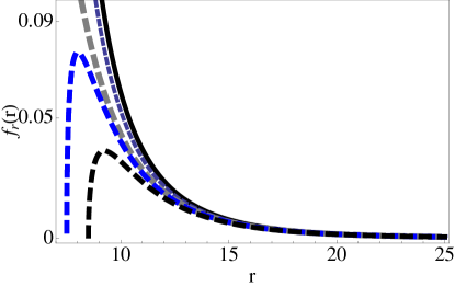
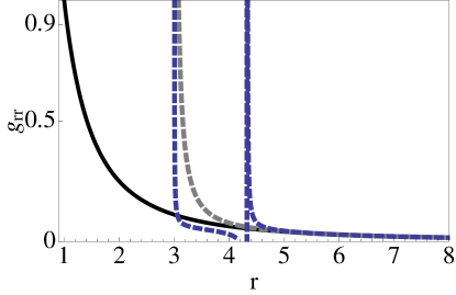
Figure 1: [Left] The behavior of the derivative of the world volume field with respect to $r$ with $L=1,r_{0}=7$, $\omega=0$ (black-solid), $\omega=5$ (dark blue-dashed), $\omega=7$ (gray-dashed), $\omega=7.5$ (blue-dashed), and $\omega=8.5$ (black-dashed). [Right] The behavior of the $g_{rr}$ component of the induced world volume metric with $L=1,r_{0}=0,\omega=0$ (black-solid), $r_{0}=3,\omega=0$ (gray-dashed), and $r_{0}=3,\omega=7.5$ (blue-dashed).

The Hawking temperature can be found from this induced metric in the form:

$$T = \frac{(g^{rr})^{\prime}}{4\pi}\bigg{|}_{r=r_{h}}=\frac{3r_{h}^{3}(r_{h}^{8}-r_{0}^{8})}{2\pi L^{2}r_{0}^{8}(6r_{h}^{2}-L^{4}\omega^{2})}=\frac{r_{h}(r_{h}^{8}-r_{0}^{8})}{2\pi\,L^{2}r_{0}^{8}}.$$ (19)

Here, as before, $r_{0}$ denotes the minimal radial extension. It is clear from (19) that at $r_{h}=r_{0}$ the temperature of the world volume black hole solution is precisely zero, $T=0$. It is also clear from (19) that the temperature increases with growing horizon size, $r_{h}>r_{0}$. Inspection of (19) also shows that the temperature of the configuration increases with decreasing the modulus $r_{0}$ (see Fig. 2). It is also clear (from Fig. 2) that when $r_{0}$ is decreased, at sufficiently large horizon size the configuration admits high temperatures. Furthermore, decreasing the value of $r_{0}$ further shows a large separation between the temperatures, $T_{r_{0}<1}/T_{r_{0}>1}\simeq 10^{8}$ (see Fig. 2). We may therefore conclude that when the size of the modulus $r_{0}$ is decreased, whereby the chiral and conformal symmetric phase is approached, the temperature increases dramatically; however, as discussed above, we note that at $r_{0}=0$ the induced world volume metric (3.1) has no thermal horizon and Hawking temperature.

We also note that by considering the backreaction of this solution to the SUGRA background, given by the KW solution $adS_{5}\times T^{1,1}$, one naturally expects the D7-brane to form a very small black hole in KW, describing a locally thermal gauge field theory in the probe limit. Accordingly, the rotating D7-brane describes a thermal object in the dual gauge field theory. In the KW example here, the system is dual to $\mathcal{N}=1$ gauge theory coupled to a quark. Since the gauge theory itself is at zero temperature while the quark is at finite temperature $T$, given by (19), the system is in non-equilibrium steady state. However, as discussed blow, the energy from the flavor sector will eventually dissipate to the gauge theory.

In the above analysis, the backreaction of the D7-brane to the supergravity background has been neglected since we considered the probe limit. It is instructive to see to what extend this can be justified. We note that the components of the stress–energy tensor of the D7-brane take the form:

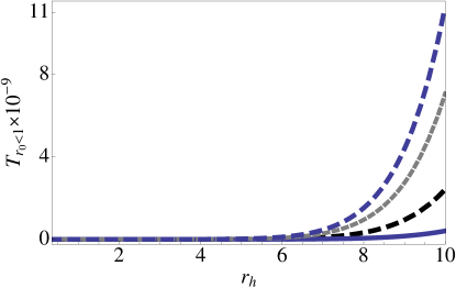
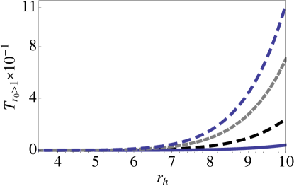
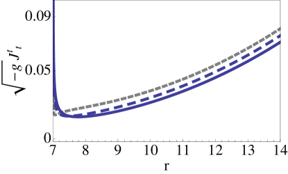
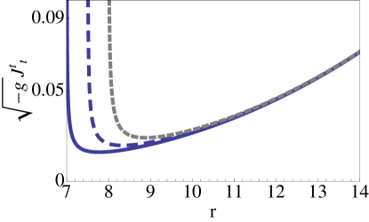
Figure 2: [Up-Left] The behavior of the temperature with $r_{0}=5$ (solid), $r_{0}=4$ (black-dashed), $r_{0}=3.5$ (gray-dashed), $r_{0}=3.3$ (blue-dashed), and $L=10$. [Up-Right] The behavior of the temperature with $r_{0}=0.5$ (solid), $r_{0}=0.4$ (black-dashed), $r_{0}=0.35$ (gray-dashed), $r_{0}=0.33$ (blue-dashed), and $L=10$. [Down-Left] The behavior of the energy-density, $\sqrt{-g}J_{t}^{t}$, with $\omega=6.8$ (gray-dashed), $\omega=5$ (dashed), $\omega=1$ (solid), and $r_{0}=7$. [Down-Right] The behavior of the energy-density with $r_{0}=8$ (gray-dashed), $r_{0}=7.5$ (dashed), $r_{0}=7$ (solid), and $\omega=1$. In all cases, $L=\alpha^{\prime}=1$ and $g_{s}=0.1$.

$$\sqrt{-g}J_{t}^{t} \equiv \frac{\tilde{T}_{D7}\,r^{3}(1+r^{2}(\phi^{\prime})^{2}/6)}{\sqrt{1+r^{2}(\phi^{\prime})^{2}/6-L^{4}\dot{\phi}^{2}/6r^{2}}}=\frac{\tilde{T}_{D7}(r^{10}-r_{0}^{8}L^{4}\overline{\omega}^{2})}{r^{2}\sqrt{(r^{8}-r_{0}^{8})(r^{2}-L^{4}\overline{\omega}^{2})}},$$ (20)

$$\sqrt{-g}J_{r}^{r} \equiv -\frac{\tilde{T}_{D7}\,r^{3}(1-L^{4}\dot{\phi}^{2}/6r^{2})}{\sqrt{1+r^{2}(\phi^{\prime})^{2}/6-L^{4}\dot{\phi}^{2}/6r^{2}}}=-\frac{\tilde{T}_{D7}}{r^{2}}\sqrt{(r^{8}-r_{0}^{8})(r^{2}-L^{4}\overline{\omega}^{2})},\;\;\$$ (21)

$$\sqrt{-g}J_{t}^{r} \equiv \frac{\tilde{T}_{D7}r^{5}\dot{\phi}\phi^{\prime}}{\sqrt{1+r^{2}(\phi^{\prime})^{2}/6-L^{4}\dot{\phi}^{2}/6r^{2}}}=\tilde{T}_{D7}r_{0}^{4}\omega^{2}.$$ (22)

Using (20)–(22), we can derive the total energy and energy flux of the D-brane system. The total energy of the D7-brane in the above configuration is given by:

$$E=\tilde{T}_{D7}\int_{r_{0}}^{\infty}{\frac{dr\,(r^{10}-r_{0}^{8}L^{4}\overline{\omega}^{2})}{r^{2}\sqrt{(r^{8}-r_{0}^{8})(r^{2}-L^{4}\overline{\omega}^{2})}}}.$$ (23)

It is clear from (23) that when $r\rightarrow r_{0}$, the energy density of the flavor brane, given by (20), becomes very large and blows up precisely at the minimal extension, $r=r_{0}$, at the IR scale of conformal and chiral flavor symmetry breaking. Thus we conclude that at the IR scale of symmetries breakdown, $r=r_{0}$, the backreaction of the D7-brane to the supergravity metric is non-negligibly large and forms a black hole centered at the IR scale $r=r_{0}$ in the bulk. The black hole size should grow as the energy is pumped into it from the D7-brane steadily. In order to obtain this energy flux, we use the components of the energy–stress tensor (20)–(22). We note that when the minimal radial extension is positive definite ($r_{0}>0$) and spin is turned on ($\omega>0$), the component (22) is non-vanishing and hence we compute the time evolution of the total energy as:

$$\dot{E}=\frac{d}{dt}\int{dr\sqrt{-g}J_{t}^{t}}=\int{dr\partial_{r}(\sqrt{-g}J_{t}^{r})}=\sqrt{-g}J_{t}^{r}|_{r=r_{0}}^{\infty}=\tilde{T}_{D7}r_{0}^{4}\omega^{2}-\tilde{T}_{D7}r_{0}^{4}\omega^{2}=0.$$ (24)

Though the total energy is time-independent, relation (24) shows that the energy (22) per unit time is injected at the boundary $r=\infty$ by some external system and the equal energy (22) is dissipated from the IR into the bulk. Such dissipation from the D7-brane to the bulk will create a black hole in the bulk. Thus, by this flow of energy form the probe to the bulk, we conclude by duality that the energy from the flavor sector will eventually dissipate into the gauge theory. In order to see explicitly this injection of energy in the stationary solution, one may set UV and IR cut offs for the rotating D7-brane solution and let the brane configuration extend from $r=r_{\text{IR}}=r_{0}$ to $r=r_{\text{UV}}\gg r_{\text{IR}}$. We note from (22) that at $r_{\text{IR}}$ and $r=r_{\text{UV}}$ the value of $T_{t}^{r}$ is non-vanishing, which shows the presence of energy flux: The incoming energy flux from $r=r_{\text{UV}}$ is given by (22) and equals that of outgoing at $r=r_{\text{IR}}$, whereat the energy does not get reflected back but its backreaction will form a black hole intaking the injected energy.

It is also instructive to inspect the parameter dependence of the solution. Inspection of (20) shows that increasing the value of $\omega$, while keeping the other parameters fixed, slightly shifts the minimum of the energy density located near the IR scale of conformal and chiral flavor symmetry breaking; it also increases the scale of the density away from the IR scale, as expected (see Fig. 2). Inspection of (20) also shows that increasing the value of $r_{0}$, while keeping the other parameters fixed, shifts the minimum of the energy density, but leaves its scale unchanged (see Fig. 2). In any case, the energy density starts from its infinite value at the IR scale, then decreases until its minimum value is reached, from where it increases to finitely small values away from the IR scale. Thus we conclude that varying the parameters of the theory leaves the overall behavior of the energy density unchanged, with the density blowing up at the IR scale, where the backreaction is non-negligible, and remaining finitely small away from the IR scale, where the backreaction can neglected.

4 Rotating D7-branes in $adS_{5}\times T^{1,1}$ in the presence of world volume gauge fields

In this section we aim to see how our analysis of the previous section gets modified at finite baryon density. In the presence of $N_{f}$ flavors, the gauge theory posses a global $U(N_{f})\simeq SU(N_{c})\times U(1)_{q}$ symmetry. The $U(1)_{q}$ counts the net number of quarks, that is, the number of baryons times $N_{c}$. In the supergravity description, this global symmetry corresponds to the $U(N_{f})$ gauge symmetry on the world volume of the $N_{f}$ D7-brane probes. The conserved currents associated with the $U(N_{f})$ symmetry of the gauge theory are dual to the gauge fields, $A_{\mu}$, on the D7-branes. Hence the introduction of a chemical potential $\mu$ or a non-vanishing $n_{B}$ for the baryon number the gauge theory corresponds to turning on the diagonal $U(1)\subset U(N_{f})$ gauge field, $A_{\mu}$ on the world volume of the D7-branes. We may describe external electric and magnetic fields in the field theory, coupled to anything having $U(1)$ charge, by introducing non-normalizable modes for $A_{\mu}$ in the supergravity theory (e.g. see ref. [17, 20]).

4.1 Induced metric and temperature in the presence of electric field

In this subsection we will study D7-branes spinning with an angular frequency $\omega$, and with a $U(1)$ world volume gauge field $A_{\mu}$. We note that in order to have the gauge theory at finite chemical potential or baryon number density, it suffices to turn on the time component of the gauge field, $A_{t}$. By symmetry considerations, one may take $A_{t}=A_{t}(r)$. As we shall briefly discuss below, a potential of this form will support an electric field.

We will consider an ansatz for the D7-brane world volume field, $\phi(r,t)=\omega t+f(r)$ and now $F_{ab}=F_{rt}=\partial_{r}A_{t}$. With this ansatz, it is straightforward to find the components of the induced world volume metric on the D7-brane, $g_{ab}^{D7}$, and compute the determinant in (7), giving the DBI Lagrangian as:

$$S_{D7}=-\tilde{T}_{D7}\int{drdt\,r^{3}\sqrt{1-\frac{L^{4}\dot{\phi}^{2}}{6r^{2}}+\frac{r^{2}\,(\phi^{\prime})^{2}}{6}-(A^{\prime}_{t}(r))^{2}}}.$$ (25)

Here we note that by setting $\dot{\phi}=\omega=0$ and $A_{t}(r)=0$, our action (25) reduces to that of the Kuperstein–Sonnenschein model, (8). As in the previous section, following the Kuperstein–Sonnenschein model reviewed in Sec. 2, we set $\theta=\pi/2$ and restrict brane motion to the equator of the $S^{2}$ sphere. Thus, in our set up we let, in addition, the probe rotate about the equator of the $S^{2}$, as before, and further turn on a non-constant world volume electric gauge field on the probe.

The equation of motion from the action (25) then take the form:

$$\frac{\partial}{\partial r}\Bigg{[}\frac{r^{5}\,\phi^{\prime}}{\sqrt{1+\frac{r^{2}\,(\phi^{\prime})^{2}}{6}-\frac{L^{4}\,\dot{\phi}^{2}}{6r^{2}}-(A^{\prime}_{t}(r))^{2}}}\Bigg{]} = \frac{\partial}{\partial t}\Bigg{[}\frac{L^{4}\,r\,\dot{\phi}}{\sqrt{1+\frac{r^{2}\,(\phi^{\prime})^{2}}{6}-\frac{L^{4}\,\dot{\phi}^{2}}{6r^{2}}-(A^{\prime}_{t}(r))^{2}}}\Bigg{]},\;\;\$$ (26)

$$\frac{\partial}{\partial r}\Bigg{[}\frac{r^{3}\,A^{\prime}_{t}(r)}{\sqrt{1+\frac{r^{2}\,(\phi^{\prime})^{2}}{6}-\frac{L^{4}\,\dot{\phi}^{2}}{6r^{2}}-(A^{\prime}_{t}(r))^{2}}}\Bigg{]} = 0.$$ (27)

Taking the large radii limit, $r\rightarrow\infty$, gives the approximate solution of the last equation as: $A_{t}(r)\simeq\mu-a_{B}/r^{2}$. Here $\mu$ is the chemical potential and $a_{B}$ is the vacuum expectation value of baryon number. We would like to remark that our solution for $A_{t}$ is of expected form. We note that an electric field will be supported by a potential of the from $A_{t}\simeq r^{-2}$. As this is a rank one massless field in $adS$, it must correspond to a dimension four operator or current in the gauge theory. This is just what one would expect from an R–current, to which gauge fields correspond. Consider rotating solutions of the form

$$\phi(r,t) = \omega t+f(r),\;\;\;\;\ f(r)=\sqrt{6}r_{0}^{4}\int_{r0}^{r}{\frac{dr}{r}\sqrt{\frac{1-L^{4}\,\overline{\omega}^{2}/r^{2}-(A^{\prime}_{t}(r))^{2}}{r^{8}-r_{0}^{8}}}}.$$ (28)

Here we note that by setting $\overline{\omega}=\omega/\sqrt{6}=0$ and $A_{t}(r)=0$, our solution (28) reduces to that of the Kuperstein–Sonnenschein model, [4], reviewed in Sec. 2 (see Eq. (9)). It is also clear that the above rotating solution has three free parameters, the minimal radial extension $r_{0}$, the angular velocity $\omega$, and the VEV of baryon number $a_{B}$. The solution (28) describes brane motion with spin and non-constant world volume electric gauge field turned on, with the brane starting and ending up at the boundary. The brane comes down from the UV boundary at infinity, bends at the minimal extension in the IR, and backs up the boundary. We also note that when $r$ is large, the behavior of the derivative of $f(r)$ with respect to $r$, denoted $f_{r}(r)$, with and without $\omega$ and world volume electric field is the same (see Fig. 3). This shows that in such limit the derivative of $f_{r}(r)$ integrates to the $\phi(r)$ of the Kuperstein–Sonnenschein model (see Sec. 2) with the boundary values $\phi_{\pm}$ in the asymptotic UV limit, $r\rightarrow\infty$ (see also Fig. 3). However, we note that in the (opposite) IR limit, i.e., when $r$ is small, the behavior of $f_{r}(r)$ does depend on $\omega$, as before. We also note here that turning on, in addition, the world volume electric field merely changes the scale but leaves the behavior of $f_{r}(r)$ in the IR unchanged. Inspection of (28) shows that in the IR only for certain values of $\omega$ the behavior of $f_{r}(r)$ with compares to that of without $\omega$ (see Fig. 3). This shows that in the IR and within specific range of $\omega>0$ the behavior of $f_{r}(r)$ (here) compares to that of $\phi^{\prime}(r)$ in the Kuperstein–Sonnenschein model (see Sec. 2), where $\phi^{\prime}(r)\rightarrow\infty$ in the IR limit $r\rightarrow r_{0}$, consistent with U-like embedding.

Again, to derive the induced metric on the D7-brane in this configuration, we put the solution (28) into the background metric (3) and obtain:

$$ds_{ind.}^{2} = -\frac{1}{3L^{2}}(3r^{2}-L^{4}\omega^{2})dt^{2}$$ (29)

$$+\frac{L^{2}}{r^{2}}\left[\frac{3r^{2}(r^{8}-r_{0}^{8})+r_{0}^{8}(6r^{2}(1-(A^{\prime}_{t}(r))^{2})-L^{4}\omega^{2})}{3r^{2}(r^{8}-r_{0}^{8})}\right]dr^{2}$$

$$+\frac{2L^{2}\omega r_{0}^{4}}{3r^{2}}\sqrt{\frac{6r^{2}(1-(A^{\prime}_{t}(r))^{2})-L^{4}\,\omega^{2}}{r^{8}-r_{0}^{8}}}drdt$$

$$+\frac{r^{2}}{L^{2}}(dx^{2}+dy^{2}+dz^{2})+\frac{L^{2}}{3}\left[\frac{1}{2}(\Omega_{1}^{2}+\Omega_{2}^{2})+\frac{1}{3}\Omega_{3}^{2}\right]$$

$$-\frac{L^{2}}{3}\left[\omega\Omega_{1}dt+\frac{r_{0}^{4}}{r^{2}}\sqrt{\frac{6r^{2}(1-(A^{\prime}_{t}(r))^{2})-L^{4}\,\omega^{2}}{r^{8}-r_{0}^{8}}}\Omega_{1}dr\right].$$

Here we note that by setting $\omega=0$ and $A_{t}(r)=0$, our induced world volume metric (29) reduces to that of the Kuperstein–Sonnenschein model, [4], reviewed in Sec. 2. In this case, for $r_{0}=0$ the induced world volume metric is that of $adS_{5}\times S^{3}$ and the dual gauge theory describes the conformal and chiral symmetric phase. On contrary, for $r_{0}>0$ the induced world volume metric has no $adS$ factor and the conformal invariance of the dual gauge theory must be broken in such case, as before. In order to find the world volume horizon and Hawking temperature, we first eliminate the relevant cross term, as before. To eliminate the relevant cross-term, we now consider a coordinate transformation:

$$\tau=t-\omega\,L^{4}r_{0}^{4}\int{\frac{dr\,(6r^{2}(1-(A^{\prime}_{t}(r))^{2})-L^{4}\,\omega^{2})^{1/2}}{r^{2}(3r^{2}-L^{4}\omega^{2})(r^{8}-r_{0}^{8})^{1/2}}}.$$ (30)

The induced metric on the rotating D7-brane(s) then takes the form:

$$ds_{ind.}^{2} = -\frac{(3r^{2}-L^{4}\omega^{2})}{3L^{2}}d\tau^{2}$$ (31)

$$+\frac{L^{2}}{r^{2}}\left[\frac{(3r^{2}-L^{4}\omega^{2})(r^{8}-r_{0}^{8})+r_{0}^{8}(6r^{2}(1-(A^{\prime}_{t}(r))^{2})-L^{4}\omega^{2})}{(3r^{2}-L^{4}\omega^{2})(r^{8}-r_{0}^{8})}\right]dr^{2}$$

$$+\frac{r^{2}}{L^{2}}(dx^{2}+dy^{2}+dz^{2})+\frac{L^{2}}{3}\left[\frac{1}{2}(\Omega_{1}^{2}+\Omega_{2}^{2})+\frac{1}{3}\Omega_{3}^{2}\right]$$

$$-\frac{L^{2}}{3}\left[\omega\Omega_{1}d\tau+\frac{3\,r_{0}^{4}}{3r^{2}-L^{4}\omega^{2}}\sqrt{\frac{6r^{2}(1-(A^{\prime}_{t}(r))^{2})-L^{4}\,\omega^{2}}{r^{8}-r_{0}^{8}}}\Omega_{1}dr\right].$$

Here we note that for $r_{0}=0$ the induced world volume metric (31) has no horizon, such that $-g_{tt}=g^{rr}=0$, and therefore not given by the black hole geometry. On contrary, for $r_{0}>0$ the induced world volume horizon is described by the horizon equation of the form:

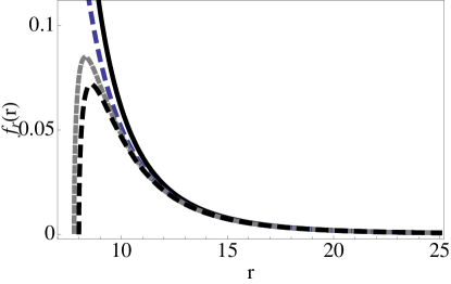
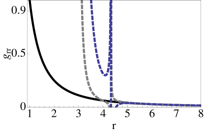
Figure 3: [Left] The behavior of the derivative of the world volume field with respect to $r$ with $L=1,r_{0}=7$, $\omega=0$ (black-solid), $\omega=5$ (blue-dashed), $\omega=7$ (gray-dashed), and $\omega=8.5$ (black-dashed). [Right] The behavior of the $g_{rr}$ component of the induced world volume metric with $L=1,r_{0}=\omega=a_{B}=0$ (black-solid), $L=1,r_{0}=3,\omega=7.5,a_{B}=20$ (gray-dashed), and $L=1,r_{0}=3,\omega=7.5,a_{B}=60$ (blue-dashed).

$$H(r)=r^{2}(r^{8}-r_{0}^{8})(3r^{2}-L^{4}\omega^{2})=0.$$ (32)

This equation is identical with Eq. (18) and therefore has the same two real positive definite zeros (see also Fig. 3). We therefore note that though the world volume electric field modifies the $g_{rr}$ component of the induced world volume metric on the rotating probe (cf. Fig. 3 $\&$ Fig. 1) the induced world volume horizon described by (32) remains unchanged compared to (18). Therefore, the thermal horizon of the induced world volume black hole geometry can be again identified with the solution of the horizon equation (32) as $-g_{tt}=g^{rr}=H(r)=3r_{h}^{2}-L^{4}\omega^{2}=0$. We therefore conclude at this point that when $r_{0}$ is positive definite ($r_{0}>0$) and spin is turned on ($\omega>0$), the induced world volume metric on the rotating probe admits a thermal horizon growing from the minimal extension $r_{0}\neq 0$ with increasing the angular velocity, unaffected by the presence of the world volume electric field.

The Hawking temperature can be found from this induced metric in the form:

$$T=\frac{(g^{rr})^{\prime}}{4\pi}\bigg{|}_{r=r_{h}}=\frac{3r_{h}^{3}(r_{h}^{8}-r_{0}^{8})}{2\pi L^{2}r_{0}^{8}[6r_{h}^{2}(1-(A^{\prime}_{t}(r))^{2})-L^{4}\omega^{2}]}=\frac{r_{h}^{7}(r_{h}^{8}-r_{0}^{8})}{2\pi L^{2}r_{0}^{8}(r_{h}^{6}-8a_{B}^{2})}.$$ (33)

From (33) it seems that the temperature of the black hole solution increases with growing horizon size, as it should. It also seems that increasing the vacuum expectation value of the baryon number density $a_{B}$ increases the temperature whereas at $a_{B}=0$ we obtain the temperature (19), as we should. However, careful inspection of (33) shows that the temperature of the solution has three distinct branches including two obvious classes of black hole solutions. First, for $a_{B}\neq 0$ and the rest of parameters fixed, the temperature $T$ decreases with increasing horizon size $r_{h}$. Here we note that as the horizon starts to grow, the temperature $T$ becomes immediately negative. Then, $T$ peeks off very sharply, producing a divergent type behavior, where at some point it hits zero, before growing into positive values. Finally, $T$ decreases positively until it reaches a non-zero minimum (see Fig. 4). In this case, the temperature of the solution seems to go more or less with the inverse of the horizon. Thus in the vicinity of the zero point the temperature of the solution decreases with increasing horizon size. These ‘small’ black holes have the familiar behavior of five-dimensional black holes in asymptotically flat spacetime, since their temperature decreases with increasing horizon size. Second, for $a_{B}\neq 0$ and the rest of parameters fixed, the other class of black hole solution appears, as the horizon size continues to grow from its value that settles the positive minimum of $T$. In this case, the temperature of the solution only increases with increasing horizon size, similar to the case with $a_{B}=0$. In this regime, we also note that increasing the VEV of $a_{B}$ increases the scale of the temperature, relative to the case $a_{B}=0$ (see Fig. 4). We also note that when we set $r_{0}<1$, the scale of $T$ increases, but its behavior remains unchanged (as in Fig. 4).

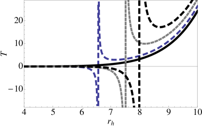
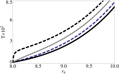
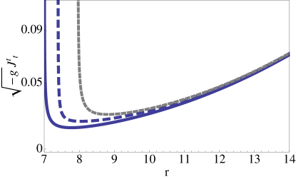
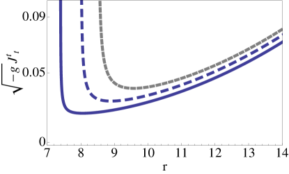
Figure 4: [Up-Left] The behavior of the temperature with $a_{B}=0$ (solid), $a_{B}=100$ (blue-dashed), $a_{B}=150$ (gray-dashed), $a_{B}=180$ (black-dashed), $L=10$ and $r_{0}=4$. [Up-Right] The behavior of the temperature with $a_{B}=0$ (solid), $a_{B}=100$ (blue-dashed), $a_{B}=150$ (gray-dashed), $a_{B}=180$ (black-dashed), $L=10$ and $r_{0}=8$. [Down-Left] The behavior of the energy-density, $\sqrt{-g}J_{t}^{t}$, with $a_{B}=0$ (solid), $a_{B}=200$ (blue-dashed), $a_{B}=250$ (gray-dashed), $r_{0}=7$, and $\omega=1$. [Down-Right] The behavior of the energy-density with $\omega=1$ (solid), $\omega=5$ (blue-dashed), $\omega=6.5$ (gray-dashed), $r_{0}=7$ and $a_{B}=200$. In these cases, $L=\alpha^{\prime}=1$ and $g_{s}=0.1$.

However, the above behavior of the temperature changes when the value of $r_{0}$ is set larger, while the rest of parameters are fixed as before. Inspection of (33) shows that when $r_{0}$ is fixed by larger values, the temperature $T$ increases continuously with increasing the horizon size $r_{h}$, and that increasing the VEV of $a_{B}$ increases the temperature $T$ (see Fig. 4). We note though that at sufficiently large horizon radii in this case $T$ scales much less than in the previous where $r_{0}$ was chosen smaller (see Fig. 4). We therefore conclude that when the external world-volume electric field is turned on, $a_{B}\neq 0$, the scale and behavior of the temperature changes according to the size of the modulus $r_{0}$. Namely, for small values of $r_{0}$, the theory admits two classes of temperatures. There is one branch where the temperature increases with increasing horizon size and there is another where the temperature decreases with increasing horizon size. At relatively larger values of $r_{0}$, there is only one branch where the temperature increases continuously with growing horizon size. In both cases, at sufficiently large horizon size the scale of the temperature increases with increasing the VEV of the baryon number density $a_{B}$.

We also note that by considering the backreaction of this solution to the KW SUGRA background, one naturally expects the D7-brane to form a very small black hole in KW, describing a locally thermal gauge field theory in the probe limit, as before. Accordingly, the rotating D7-brane describes a thermal object in the dual gauge field theory. In the KW example here, the system is dual to $\mathcal{N}=1$ gauge theory coupled to a quark in the presence of an external electric field. Since the gauge theory itself is at zero temperature while the quark is at finite temperature $T$, (33), the system is in non-equilibrium steady state. However, as discussed below, the energy from the flavor sector will eventually dissipate into the gauge theory, as before.

In the above analysis, the backreaction of the D7-brane to the supergravity background has been neglected since we considered the probe limit. It is instructive to see to what extend this can be justified. The components of the stress–energy tensor of the D7-brane take the form:

$$\sqrt{-g}J_{t}^{t} \equiv \frac{\tilde{T}_{D7}\,r^{3}(1+r^{2}(\phi^{\prime})^{2}/6)}{\sqrt{1+r^{2}(\phi^{\prime})^{2}/6-L^{4}\dot{\phi}^{2}/6r^{2}-(A^{\prime})^{2}}}$$ (34)

$$= \frac{\tilde{T}_{D7}(r^{4}(r^{10}-L^{4}\overline{\omega}^{2}r_{0}^{8})-4r_{0}^{8}a_{B}^{2})}{r^{4}\sqrt{(r^{8}-r_{0}^{8})(r^{6}-L^{4}\overline{\omega}^{2}r^{4}-4a_{B}^{2})}},\;\;\;\;\;\;\;\;\$$

$$\sqrt{-g}J_{r}^{r} \equiv -\frac{\tilde{T}_{D7}\,r^{3}(1-L^{4}\dot{\phi}^{2}/6r^{2})}{\sqrt{1+r^{2}(\phi^{\prime})^{2}/6-L^{4}\dot{\phi}^{2}/6r^{2}-(A^{\prime})^{2}}}$$ (35)

$$= -\tilde{T}_{D7}(r^{2}-L^{4}\overline{\omega}^{2})\sqrt{\frac{r^{8}-r_{0}^{8}}{r^{6}-L^{4}\overline{\omega}^{2}r^{4}-4a_{B}^{2}}},$$

$$\sqrt{-g}J_{t}^{r} \equiv \frac{\tilde{T}_{D7}r^{5}\dot{\phi}\phi^{\prime}}{\sqrt{1+r^{2}(\phi^{\prime})^{2}/6-L^{4}\dot{\phi}^{2}/6r^{2}-(A^{\prime})^{2}}}=\tilde{T}_{D7}r_{0}^{4}\omega.$$ (36)

Using (34)–(36), we can derive the total energy and energy flux of the D-brane system. The total energy of the D7-brane in the above configuration is given by:

$$E=\tilde{T}_{D7}\int_{r_{0}}^{\infty}{\frac{dr\,(r^{4}(r^{10}-L^{4}\overline{\omega}^{2}r_{0}^{8})-4r_{0}^{8}a_{B}^{2})}{r^{4}\sqrt{(r^{8}-r_{0}^{8})(r^{6}-L^{4}\overline{\omega}^{2}r^{4}-4a_{B}^{2})}}}.$$ (37)

It is straightforward to see that when the electric field is tuned off, (34)–(37) reduce to (20)–(23), as they should. It is also clear from (37) that when $r\rightarrow r_{0}$, the energy density of the flavor brane, given by (34), becomes very large and blows up precisely at the minimal extension, $r=r_{0}$, at the IR scale of conformal and chiral flavor symmetry breaking, independent from the presence of the world volume electric field. Thus we conclude that at the IR scale of symmetries breakdown, $r=r_{0}$, the backreaction of the D7-brane to the supergravity metric is non-negligibly large and forms a black hole centered at the IR scale $r=r_{0}$ in the bulk, as before. The black hole size should grow as the energy is pumped into it from the D7-brane steadily. In order to obtain this energy flux, we use the components of the energy–stress tensor (34)–(36). We note that when the minimal radial extension is positive definite ($r_{0}>0$) and spin is turned on ($\omega>0$), the component (36) is non-vanishing and hence we compute the time evolution of the total energy as:

$$\dot{E}=\frac{d}{dt}\int{dr\sqrt{-g}J_{t}^{t}}=\int{dr\partial_{r}(\sqrt{-g}J_{t}^{r})}=\sqrt{-g}J_{t}^{r}|_{r=r_{0}}^{\infty}=\tilde{T}_{D7}r_{0}^{4}\omega^{2}-\tilde{T}_{D7}r_{0}^{4}\omega^{2}=0.$$ (38)

Here we note that when the electric field is turned on, (36) and energy dissipation (38) remain unchanged, compared with (22) and (24). Therefore, independent from the electric field, the energy dissipation from the brane into the bulk will form a black hole, centered at the IR scale $r=r_{0}$, as before (see Sec. 3.1). Thus, by this flow of energy form the probe to the bulk, we conclude by duality that the energy from the flavor sector will eventually dissipate into the gauge theory, independent from the electric field. To see this external injection of energy in our stationary rotating solution, we may again adopt UV/IR cut offs and find from (36) that, independent from the electric field, at $r=r_{\text{IR}}$ the energy is unreflected back but its backreaction will form a black hole, absorbing the injected energy, as before (see Sec. 3.1).

It is also instructive to inspect the parameter dependence of the theory in the presence of the electric field. Inspection of (34) shows that when the electric field in turned on, the scale and behavior of the energy density remains unchanged (see Fig. 4). Inspection of (34) shows that increasing $a_{B}$ by relatively large values, while keeping the rest of parameters fixed, merely shifts the minimum of the energy density (see Fig. 4). Inspection of (34) also shows that increasing the value of the angular velocity $\omega$, while keeping the rest of parameters fixed, increases the energy density, as expected (see Fig. 4). However, the energy density is increased such that the backreaction remains negligibly small away from the blowing up point (see Fig. 4). Thus we conclude that in the presence of the electric field varying the parameters of the theory leaves the behavior of the energy density more or less unchanged, with the density blowing up at the IR scale, where the backreaction is non-negligible, and remaining finitely small elsewhere, where the backreaction is negligible.

4.2 Induced metric and temperature in the presence of magnetic field

In this subsection we will study D7-branes spinning with an angular frequency $\omega$, and with a $U(1)$ world volume gauge field $A_{\mu}$, but in place of turning on an electric field, we will be interested in a magnetic field, which we may introduce through adding to our D7-brane ansatz the constant magnetic field $F_{xy}=B$. In the gauge theory, one can identify $F_{xy}$ as a constant $U(1)$ magnetic field pointing in the z direction. The relevance of introducing $B$ is that at zero temperature, zero mass, and zero R–charge chemical potential, gauge/gravity calculations have shown that such a $U(1)$ $B$-field triggers spontaneous breaking of the R–symmetry [20]. However, we are interested in solutions at finite R–charge chemical potential and $U(1)$ magnetic field. Such solutions describe states in the gauge theory with degenerate hypermultiplet fields, a finite R–charge density, and spontaneous breaking of the R–symmetry.

We will consider an ansatz for the D7-brane world volume field $\phi(r,t)=\omega t+f(r)$ and now $F_{xy}=B$. With this ansatz, it is straightforward to find the components of the induced world volume metric on the D7-brane, $g_{ab}^{D7}$, and compute the determinant in (7), giving the DBI Lagrangian as:

$$S_{D7}=-\tilde{T}_{D7}\int{drdt\,r^{3}\sqrt{\bigg{(}1+\frac{L^{4}\hat{B}^{2}}{r^{4}}\bigg{)}\bigg{(}1-\frac{L^{4}\dot{\phi}^{2}}{6r^{2}}+\frac{r^{2}\,(\phi^{\prime})^{2}}{6}\bigg{)}}}.$$ (39)

Here we note that by setting $\dot{\phi}=\omega=0$ and $\hat{B}=(2\pi\alpha^{\prime})B=0$, our action (39) reduces to that of the Kuperstein–Sonnenschein model, (8). As in the previous sections, following the Kuperstein–Sonnenschein model reviewed in Sec. 2, we set $\theta=\pi/2$ and restrict brane motion to the equator of the $S^{2}$ sphere. Thus, in our set up we let, in addition, the probe rotate about the equator of the $S^{2}$, as before, and further turn on a constant world volume magnetic gauge field on the probe.

The equation of motion from the action (39) takes then the form:

$$\frac{\partial}{\partial r}\left[\frac{r^{5}\,(1+L^{4}\hat{B}^{2}/r^{4})\,\phi^{\prime}}{\sqrt{(1+L^{4}\hat{B}^{2}/r^{4})(1-L^{4}\dot{\phi}^{2}/6r^{2}+r^{2}(\phi^{\prime})^{2}/6)}}\right] =$$

$$\frac{\partial}{\partial t}\left[\frac{L^{4}r\,(1+L^{4}\hat{B}^{2}/r^{4})\dot{\phi}}{\sqrt{(1+L^{4}\hat{B}^{2}/r^{4})(1-L^{4}\dot{\phi}^{2}/6r^{2}+r^{2}\,(\phi^{\prime})^{2}/6}}\right].$$ (40)

Consider rotating solutions of the form

$$\phi(r,t) = \omega t+f(r),\;\;\;\;\ f(r)=\sqrt{6}r_{0}^{4}\int_{r_{0}}^{r}{\frac{dr}{r}\sqrt{\frac{1-L^{4}\overline{\omega}^{2}/r^{2}}{r^{6}(r^{2}+L^{4}\hat{B}^{2})-r_{0}^{8}}}}.$$ (41)

Here we note that by setting $\overline{\omega}=\omega/\sqrt{6}=0$ and $\hat{B}=0$, our solution (41) reduces to that of the Kuperstein–Sonnenschein model, [4], reviewed in Sec. 2 (see Eq. (9)). It is also clear that the above rotating solution has three free parameters, the minimal radial extension $r_{0}$, the angular velocity $\omega$, and the value of the magnetic field $B$. The solution (41) describes brane motion with spin and constant world volume magnetic gauge field turned on, with the brane starting and ending up at the boundary. The brane comes down from the UV boundary at infinity, bends at the minimal extension in the IR, and backs up the boundary. We also note that when $r$ is large, the behavior of the derivative of $f(r)$ with respect to $r$, denoted $f_{r}(r)$, with and without $\omega$ and world volume electric field is the same (see Fig. 4). This shows that in such limit the derivative of $f_{r}(r)$ integrates to the $\phi(r)$ of the Kuperstein–Sonnenschein model (see Sec. 2) with the boundary values $\phi_{\pm}$ in the asymptotic UV limit, $r\rightarrow\infty$ (see also Fig. 4). However, we note that in the (opposite) IR limit, i.e., when $r$ is small, the behavior of $f_{r}(r)$ does depend on $\omega$ and $B$. Inspection of (41) shows that in the IR only for certain values of $\omega$ and $B$ the behavior of $f_{r}(r)$ with compares to that of without $\omega$ and $B$ (see Fig. 4). This shows that in the IR and within specific range of $\omega,B>0$ the behavior of $f_{r}(r)$ (here) compares to that of $\phi^{\prime}(r)$ in the Kuperstein–Sonnenschein model (see Sec. 2), where $\phi^{\prime}(r)\rightarrow\infty$ in the IR limit $r\rightarrow r_{0}$, consistent with U-like embedding.

As before, to derive the induced metric on the D7-brane in this configuration, we put the rotating solution (41) into the background metric (3) and obtain:

$$ds_{ind.}^{2} = -\frac{1}{3L^{2}}(3r^{2}-L^{4}\omega^{2})dt^{2}$$

$$+\frac{L^{2}}{r^{2}}\left[\frac{3r^{2}(r^{6}(r^{2}+L^{4}\hat{B}^{2})-r_{0}^{8})+r_{0}^{8}(6r^{2}-L^{4}\omega^{2})}{3r^{2}(r^{6}(r^{2}+L^{4}\hat{B}^{2})-r_{0}^{8})}\right]dr^{2}$$

$$+\frac{2L^{2}\omega\,r_{0}^{4}}{3r^{2}}\sqrt{\frac{6r^{2}-L^{4}\,\omega^{2}}{r^{6}(r^{2}+L^{4}\hat{B}^{2})-r_{0}^{8}}}drdt+\frac{r^{2}}{L^{2}}(dx^{2}+dy^{2}+dz^{2})$$

$$+\frac{L^{2}}{3}\left[\frac{1}{2}(\Omega_{1}^{2}+\Omega_{2}^{2})+\frac{1}{3}\Omega_{3}^{2}-\omega\Omega_{1}dt-\frac{r_{0}^{4}}{r^{2}}\sqrt{\frac{6r^{2}-L^{4}\,\omega^{2}}{r^{6}(r^{2}+L^{4}\hat{B}^{2})-r_{0}^{8}}}\Omega_{1}dr\right].$$

Here we note that by setting $\omega=0$ and $B=0$, our induced world volume metric (4.2) reduces to that of the Kuperstein–Sonnenschein model, [4], reviewed in Sec. 2. In this case, for $r_{0}=0$ the induced world volume metric is that of $adS_{5}\times S^{3}$ and the dual gauge theory describes the conformal and chiral symmetric phase. On contrary, for $r_{0}>0$ the induced world volume metric has no $adS$ factor and the conformal invariance of the dual gauge theory must be broken in such case, as before. In order to find the world volume horizon and Hawking temperature, we first eliminate the relevant cross term, as before. To eliminate the relevant cross-term, we now consider a coordinate transformation:

$$\tau=t-\omega\,L^{4}r_{0}^{4}\int{\frac{dr\,(6r^{2}-L^{4}\,\omega^{2})^{1/2}}{r^{2}(3r^{2}-L^{4}\omega^{2})(r^{6}(r^{2}+L^{4}\hat{B}^{2})-r_{0}^{8})^{1/2}}}.$$ (43)

The induced metric on the rotating D7-brane(s) then takes the form:

$$ds_{ind.}^{2} = -\frac{(3r^{2}-L^{4}\omega^{2})}{3L^{2}}d\tau^{2}$$ (44)

$$+\frac{L^{2}}{r^{2}}\left[\frac{(3r^{2}-L^{4}\omega^{2})(r^{6}(r^{2}+L^{4}\hat{B}^{2})-r_{0}^{8})+r_{0}^{8}(6r^{2}-L^{4}\omega^{2})}{(3r^{2}-L^{4}\omega^{2})(r^{6}(r^{2}+L^{4}\hat{B}^{2})-r_{0}^{8})}\right]dr^{2}$$

$$+\frac{r^{2}}{L^{2}}(dx^{2}+dy^{2}+dz^{2})+\frac{L^{2}}{3}\left[\frac{1}{2}(\Omega_{1}^{2}+\Omega_{2}^{2})+\frac{1}{3}\Omega_{3}^{2}\right]$$

$$-\frac{L^{2}}{3}\left[\omega\Omega_{1}d\tau+\frac{3\,r_{0}^{4}}{3r^{2}-L^{4}\omega^{2}}\sqrt{\frac{6r^{2}-L^{4}\,\omega^{2}}{r^{6}(r^{2}+L^{4}\hat{B}^{2})-r_{0}^{8}}}\Omega_{1}dr\right].$$

Here we note that for $r_{0}=0$ the induced world volume metric (31) has no horizon, such that $-g_{tt}=g^{rr}=0$, and therefore not given by the black hole geometry. On contrary, for $r_{0}>0$ the induced world volume horizon is described by the the horizon equation of the form:

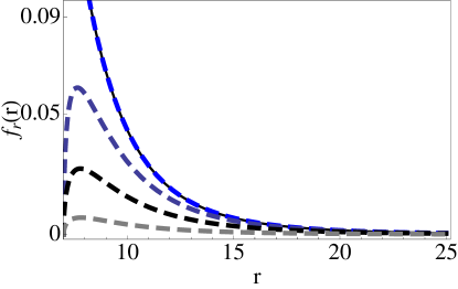
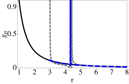
Figure 5: [Left] The behavior of the derivative of the world volume field with respect to $r$ with $L=1,r_{0}=7,\omega=7,$, $B=0$ (black-solid), $B=0.05$ (blue-dashed), $B=10$ (dark blue-dashed), $B=25$ (black-dashed), and $B=100$ (gray-dashed). [Right] The behavior of the $g_{rr}$ component of the induced world volume metric with $L=1,r_{0}=\omega=B=0$ (black-solid), $L=1,r_{0}=3,\omega=7.5$, $B=0.05$ (gray-dashed), and $B=25$ (blue-dashed).

$$H(r)=r^{2}(r^{6}(r^{2}+L^{4}B^{2})-r_{0}^{8})(3r^{2}-L^{4}\omega^{2})=0.$$ (45)

This equation, unlike (32), is not the same as (18), though it has some similar features. We note that the world volume magnetic field modifies the $g_{rr}$ component of the induced world volume metric (see Fig. 5) as well as the induced world volume horizon described by (45), though the thermal horizon can be identified with the solution of (45) as $-g_{tt}=g^{rr}=H(r)=3r^{2}-L^{4}\omega^{2}=0$, as before. However, we note that by setting $B$ large, the induced world volume horizon described by (45) appears to start from zero. In other words, by setting $B$ large and demanding the world volume horizon to start from the minimal radial extension $r_{0}$, the horizon equation (45) implies $r_{0}=0$. This may indicate that when the world volume magnetic field is turned on, the world volume horizon has to start from the conifold point, $r=r_{0}=0$, whereby the induced world volume horizon is inside the $adS$ horizon. But, we saw that for $r_{0}=0$ the induced world volume metric (44), has no thermal horizon, to begin with. And, we note that in U-like embeddings the point $r_{0}=0$ is outside the validity range of the induced world volume metric (44). Nevertheless, closer inspection of the horizon equation (45) shows that when $B$ is set small, the world volume horizon starts nearly from $r_{0}\neq 0$. We therefore conclude at this point that when the minimal extension is positive definite ($r_{0}>0$) and spin is turned on ($\omega>0$) and the world volume magnetic field ($B=const.$) is induced, the induced world volume metric admits a thermal horizon growing almost from $r_{0}$ with increasing the angular velocity, provided that the magnetic field is weak.

The Hawking temperature can be found from this induced metric in the form:

$$T=\frac{(g^{rr})^{\prime}}{4\pi}\bigg{|}_{r=r_{h}}=\frac{3r_{h}^{3}[r_{h}^{4}(r_{h}^{4}+L^{4}\hat{B}^{2})-r_{0}^{8}]}{2\pi L^{2}r_{0}^{8}(6r_{h}^{2}-L^{4}\omega^{2})}=\frac{r_{h}[r_{h}^{4}(r_{h}^{4}+L^{4}\hat{B}^{2})-r_{0}^{8}]}{2\pi L^{2}r_{0}^{8}}.$$ (46)

From (46) it is clear that the temperature of the black hole solution increases with growing horizon size. It is also clear that increasing the magnetic field $B$ increases the temperature whereas at $B=0$ we obtain the temperature (19), as we should. We also note that in the presence of the magnetic field, $B\neq 0$, at $r_{h}=r_{0}$ there is a minimum temperature, below which there is no world volume black hole solution on the probe. This is unlike in previous examples where the minimum temperature was zero. The minimum temperature, in this case, goes with quadric of $B$ and with inverse cube of $r_{0}$, $T_{0}=(L\,\hat{B})^{2}/2\pi r_{0}^{3}$. This shows that for fixed values of $L$ the size of the minimum temperature $T_{0}$ increases with increasing $B$ and decreasing $r_{0}$. Inspection of (46) also shows that when the magnetic field is turned on, the temperature of the world volume black hole solution increases continuously with growing horizon size (see Fig. 6). This qualitative behavior is independent from the choice of parameters. Comparison with Sec. 1 also shows that increasing the value of the magnetic field, while $r_{0}$ is fixed, affects the scale of the temperature by more or less the same amount as decreasing $r_{0}$ does, while the magnetic field is turned off, with the same large hierarchy $T_{r_{0}>1}/T_{r_{0}<1}\simeq 10^{8}$ (see Fig. 6 and Fig. 2). Comparison with Sec. 1 also shows that that in the presence of the magnetic field the behavior of the temperature remains the same. This is in contrast with Sec. 3 where the presence of the electric field modified the behavior of the temperature (see Fig. 6, Fig. 4 and Fig. 2). We therefore conclude that when the world-volume magnetic field $B$ is turned on, the temperature $T$ grows from its minimum $T_{0}$, with the scale of $T$ increased, while its behavior remains unchanged, as $B$ is increased at any fixed $r_{0}$.

We also note that by considering the backreaction of this solution to the KW SUGRA background, one naturally expects the D7-brane to form a very small black hole in KW, describing a locally thermal gauge field theory in the probe limit, as before. Accordingly, the rotating D7-brane describes a thermal object in the dual gauge field theory. In the KW example here, the system is dual to $\mathcal{N}=1$ gauge theory coupled to a quark in the presence of an external magnetic field. Since the gauge theory itself is at zero temperature while the quark is at finite temperature $T$, given by (46), the system is in non-equilibrium steady state. However, as discussed below, the energy from the flavor sector will eventually dissipate to the gauge theory, as before.

In the above analysis, the backreaction of the D7-brane to the supergravity background has been neglected since we considered the probe limit. It is instructive to see to what extend this can be justified. The components of the stress–energy tensor of the D7-brane take the form:

$$\sqrt{-g}J_{t}^{t} \equiv \frac{\tilde{T}_{D7}\,r^{3}(1+L^{4}\tilde{B}^{2}/r^{4})^{1/2}(1+r^{2}(\phi^{\prime})^{2}/6)}{\sqrt{1+r^{2}(\phi^{\prime})^{2}/6-L^{4}\dot{\phi}^{2}/6r^{2}}}$$ (47)

$$= \frac{\tilde{T}_{D7}[r^{6}(r^{4}+L^{4}\tilde{B}^{2})-r_{0}^{8}L^{4}\overline{\omega}^{2}]}{r^{4}}\sqrt{\frac{r^{4}+L^{4}\tilde{B}^{2}}{[r^{4}(r^{4}+L^{4}\tilde{B}^{2})-r_{0}^{8}][r^{2}-L^{4}\overline{\omega}^{2}]}},\;\;\;\$$

$$\sqrt{-g}J_{r}^{r} \equiv -\frac{\tilde{T}_{D7}\,r^{3}(1+L^{4}\tilde{B}^{2}/r^{4})^{1/2}(1-L^{4}\dot{\phi}^{2}/6r^{2})}{\sqrt{1+r^{2}(\phi^{\prime})^{2}/6-L^{4}\dot{\phi}^{2}/6r^{2}}}$$ (48)

$$= -\frac{\tilde{T}_{D7}}{r^{2}}\sqrt{(r^{2}-L^{4}\overline{\omega}^{2})[r^{4}(r^{4}+L^{4}\tilde{B}^{2})-r_{0}^{8}]},$$

$$\sqrt{-g}J_{t}^{r} \equiv \frac{\tilde{T}_{D7}r^{5}(1+L^{4}\tilde{B}^{2}/r^{4})^{1/2}\dot{\phi}\phi^{\prime}}{\sqrt{1+r^{2}(\phi^{\prime})^{2}/6-L^{4}\dot{\phi}^{2}/6r^{2}}}=\tilde{T}_{D7}r_{0}^{4}\omega.$$ (49)

Using (47)–(49), we can derive the total energy and energy dissipation of the system. The total energy of the D7-brane in the above configuration is given by:

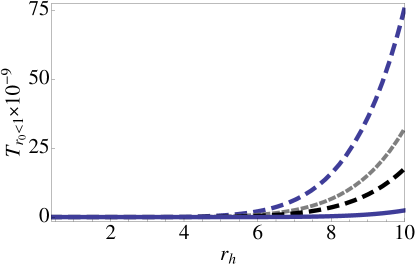
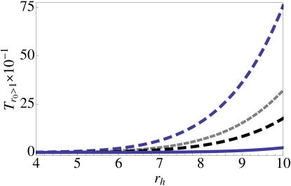
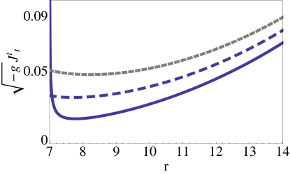
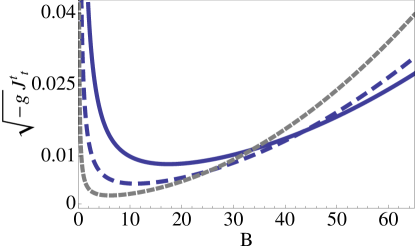
Figure 6: [Up-Left] The behavior of the temperature with $B=0$ (solid), $B=0.25$ (black-dashed), $B=0.35$ (gray-dashed), $B=0.55$ (blue-dashed), $L=10$ and $r_{0}=4$. [Up-Right] The behavior of the temperature with $r_{0}=0.4$ and the same values of $B$. [Down-Left] The behavior of the energy-density, $\sqrt{-g}J_{t}^{t}$, with $B=0$ (solid), $B=70$ (dashed), $B=100$ (gray-dashed), and $r_{0}=7$. [Down-Right] The behavior of the energy-density with $r_{0}=5$ (solid), $r_{0}=4$ (dashed), $r_{0}=3$ (gray-dashed). Here: $L=\alpha^{\prime}=\omega=1$, and $g_{s}=0.1$.

$$E=\tilde{T}_{D7}\int_{r_{0}}^{\infty}{\frac{dr\,[r^{6}(r^{4}+L^{4}\tilde{B}^{2})-r_{0}^{8}L^{4}\overline{\omega}^{2}]}{r^{4}}\sqrt{\frac{r^{4}+L^{4}\tilde{B}^{2}}{[r^{4}(r^{4}+L^{4}\tilde{B}^{2})-r_{0}^{8}][r^{2}-L^{4}\overline{\omega}^{2}]}}}.$$ (50)

It is easy to see that when the magnetic field is tuned off, $B=0$, (47)–(50) reduce to (20)–(23), as they should. It is also clear form (50) that in the presence of the magnetic field, $B\neq 0$, the value of the energy density, given by (47), remains finite at the IR scale $r=r_{0}$, on contrary with the previous examples (Secs. 3.1 $\&$ 4.1). Nonetheless, closer inspection of the denominator of (47) shows that when the magnetic field $B$ is not too large, compared with other scales of the theory, the energy density does blow up instead in the vicinity of the minimal extension $r=r_{0}$, nearby the IR scale of conformal and chiral flavor symmetry breaking. Thus we conclude that close to the IR scale of symmetries breakdown $r=r_{0}$, the backreaction of the D7-brane to the supergravity background metric is non-negligibly large and forms a black hole centered nearby the IR scale $r=r_{0}$ in the bulk. The black hole size should grow as the energy is pumped into it from the D7-brane steadily. In order to obtain this energy flux, we note that the components of the energy–stress tensor are given by (47–(49). We note that when the minimal radial extension is positive definite ($r_{0}>0$) and spin is turned on ($\omega>0$), the component (49) is non-vanishing and hence we compute the time evolution of the total energy as:

$$\dot{E}=\frac{d}{dt}\int{dr\sqrt{-g}J_{t}^{t}}=\int{dr\partial_{r}(\sqrt{-g}J_{t}^{r})}=\sqrt{-g}J_{t}^{r}|_{r=r_{0}=0}^{\infty}=\tilde{T}_{D7}r_{0}^{4}\omega^{2}-\tilde{T}_{D7}r_{0}^{4}\omega^{2}=0.$$ (51)

Here we note that when the magnetic field is turned on, the component (49) and energy dissipation relation (51) remain unchanged, compared with (22) and (24), as in the previous example (Sec. 3.1). Therefore, independent from the magnetic field, the energy dissipation from the brane into the bulk will form a black hole centered nearby the IR scale $r=r_{0}$, as before (see Secs. 3.1 $\&$ 4.1). Thus, by this flow of energy from the brane into the bulk, we conclude by duality that the energy from the flavor sector will eventually dissipate into the gauge theory, independent from the magnetic field. To see this external injection of energy in our stationary rotating solution, we may again consider UV and IR cut offs and find from (49) that, independent from the magnetic field, at $r=r_{\text{IR}}$ the energy is unreflected back but its backreaction will form a black hole, absorbing the injected energy, as before (see Secs. 3.1 $\&$ 4.1).

It is also instructive to inspect the parameter dependence of the theory in the presence of the magnetic field. Inspection of (47) shows that when the magnetic field is turned on, the energy density increases (see Fig. 6). However, inspection of (47) shows that increasing the magnetic field $B$ by relatively large values, while keeping the rest of parameters fixed, increases the energy density and hence the backreaction, though such that the backreaction remains negligibly small away from the blowing up point (see Fig. 6). Inspection of (47) also shows that at the IR scale $r=r_{0}$ the energy densities with different values of $r_{0}$, and other parameters fixed, become degenerate for certain values of the magnetic field (see Fig. 6). Thus we conclude that in the presence of the magnetic field varying the parameters of the theory leaves the overall behavior of the energy density more or less unchanged, with the density blowing up nearby the IR scale, where the backreaction is non-negligible, and remaining finitely small elsewhere, where the backreaction is negligible.

5 Discussion

In this paper, we studied, in detail, the induced world volume metrics and Hawking temperatures of rotating probe D7-branes in the Kuperstein–Sonnenschein holographic model. We also studied, in detail, the energy–stress tensors and energy flow of rotating probe D7-branes in the Kuperstein–Sonnenschein model. By gauge/gravity duality, the Hawking temperatures on the rotating probe D7-branes in supergravity correspond to the temperatures of flavored quarks in the gauge theory, and the energy flow from the probe D7-brane into the system, to the energy dissipation from the flavor sector into the gauge theory. Such non-equilibrium systems and their energy dissipation have already been studied in the literature in conformal $adS$ setups. The aim of this work was to extend such previous analyses to more general and realistic holographic setups. The motivation of this work was to construct novel examples of non-equilibrium steady states in holographic models where the conformal and chiral flavor symmetry of the dual gauge theory get spontaneously broken.

We derived the induced world volume metrics on rotating probe D7-branes, with and without the presence of worldvolume gauge fields, in the Kuperstein–Sonnenschein model. We showed that when the minimal extension of the probe is positive definite and spin is turned on, the induced world volume metrics on the rotating probe admit thermal horizons and Hawking temperatures despite the absence of black holes in the bulk. We found that the scale and behavior of the probe temperature are determined strongly by the size of the minimal extension of the probe, and by the strength and sort of world volume gauge fields. By duality, we thus found the scale and behavior of temperature in flavored quarks are strongly determined by the IR scale of symmetries breakdown, and by the strength and sort of external fields. We noted that by considering the backreaction of such solutions to the holographic background, one naturally expects the D7-brane to form a very small black hole in the background, corresponding to a locally thermal gauge field theory in the probe limit. We thus found the rotating probe D7-brane describing a thermal object in the dual gauge field theory, including a quark, with or without the presence of external fields. Because the gauge theory itself was at zero temperature while the quark was at finite temperature, we found that such systems are in non-equilibrium steady states. However, we found that in the IR the backreaction is large and the energy will dissipate from the probe D7-brane into the bulk. By duality, we thus found the energy dissipation from the flavor sector into the gauge theory.

In the absence of the world volume gauge fields, we found that the world volume horizon starts from the minimal extension and grows with increasing the angular velocity. We found the temperature increasing steadily from zero with the horizon size growing from the minimal extension. We also found that the scale of the temperature increases/decreases dramatically, while its behavior remains unchanged, when the minimal extension is decreased/increased. We thus found, in this example, that the temperature is determined by the shape of flavor brane embedding configuration: ‘sharp’ U-like configurations–approaching V-like–($r_{0}<1$) admit higher temperatures than ‘smooth’ U-likes ($r_{0}>1$). This may be expected, since by decreasing the minimal extension the conformal and chiral symmetric phase is approached. However, we saw that when the configuration is V-like ($r_{0}=0$), corresponding to the conformal and chiral symmetric phase, the induced world volume metric on the rotating probe admits no thermal horizon and hence no Hawking temperature. We noted that by considering the backreaction of this solution to the KW SUGRA background, one naturally expects the D7-brane to form a very small black hole in KW, corresponding to a locally thermal gauge field theory in the probe limit. Accordingly, we found the rotating probe D7-brane describing a thermal object in the dual gauge field theory. In this example, the system was dual to $\mathcal{N}=1$ gauge theory coupled to a quark. Since the gauge theory itself was at zero temperature while the quark is at finite temperature, we found, in this example, that the system is in non-equilibrium steady state. However, we then showed that the energy from the flavor sector will eventually dissipate into the gauge theory. We first found from the energy–stress tensor that, independent from the choice of parameters, at the minimal extension, at the IR scale of conformal and chiral flavor symmetry breakdown, the energy density blows up and hence showed the backreaction in the IR is non-negligible. We then showed from the energy–stress tensor that when the minimal extension is positive definite and spin is turned on, the energy flux is non-vanishing and found the energy can flow from the D7-brane into the bulk, forming, with the large backreaction, a black hole in the bulk. We also argued how this external injection of energy may be understood in our stationary solutions. We considered UV and IR cut offs in our rotating D7-brane system and noted from the energy–stress tensor that the incoming energy from the UV equals the outgoing energy from the IR where the large backreaction forms a black hole intaking the injected energy. By gauge/gravity duality, we thus found, in this example, the energy dissipation from the flavor sector into the gauge theory.

In the presence of the world volume electric field, we first found that both the behavior as well as the scale of the temperature get modified. We found that turning on the world volume electric field renders the temperature described by two distinct branches. We found that there is one branch where the temperature increases and another where it decreases with increasing the horizon size. While the former branch is rather of usual form, the latter describes ‘small’ black holes. However, we then varied the parameters of the theory and found that the two distinct branches appear only for certain set of parameters. We found that for relatively larger values of the minimal extension the temperature only increases with increasing horizon size. We also found that at sufficiently large horizon size, for any fixed value of the minimal extension, increasing the VEV of the baryon density number increases the scale of the temperature. We noted that by considering the backreaction of this solution to the KW SUGRA background, one naturally expects the D7-brane to form a very small black hole in KW, corresponding to a locally thermal gauge field theory in the probe limit. Accordingly, we found the rotating D7-brane describing a thermal object in the dual gauge field theory. In this example, the system was dual to $\mathcal{N}=1$ gauge theory coupled to a quark in the presence of an external electric field. Since the gauge theory itself was at zero temperature while the quark is at finite temperature, we found, in this example, that the system is in non-equilibrium steady state. However, we then showed that the energy from the flavor sector will eventually dissipate into the gauge theory. We first found from the energy–stress tensor that, independent from the VEV of baryon density number and the choice of other parameters, at the minimal extension, at the IR scale of conformal and chiral flavor symmetry breakdown, the energy density blows up and so showed the backreaction in the IR is non-negligible. We then showed from the energy–stress tensor that when the minimal extension is positive definite and spin is turned on, the energy flux is non-vanishing and found the energy can flow from the brane into the bulk, forming, with the large backreaction, a black hole in the bulk, independent from the presence of the electric field. We also argued how this external injection of energy may be understood in our stationary solutions, by setting UV and IR cut offs in our rotating D7-brane system, as before. By gauge/gravity duality, we thus found, in this example, the energy dissipation from the flavor sector into the gauge theory, independent from the electric field.

In the presence of the world volume magnetic field, we found that only the scale of the temperature changes. We found that when the magnetic field is turned on, the temperature has a minimum below which there is no black hole solution. We found the temperature increasing steadily from its minimum with growing horizon size. We also showed that increasing the magnetic field increases the scale of the temperature, but leaves its behavior unchanged. We found the increase in the temperature due to increasing the magnetic field similar to the increase in the temperature due to decreasing the minimal extension with the world volume gauge fields turned off. We noted that by considering the backreaction of this solution to the KW SUGRA background, one naturally expects the D7-brane to form a very small black hole in KW, corresponding to a locally thermal gauge theory in the probe limit. Therefore, we found the rotating D7-brane describing a thermal object in the dual gauge field theory. In this example, the system was dual to $\mathcal{N}=1$ gauge theory coupled to a quark in the presence of an external magnetic field. Since the gauge theory itself was at zero temperature while the quark is at finite temperature, we found, in this example, that the system is in non-equilibrium steady state. However, we then showed that the energy from the flavor sector will eventually dissipate into the gauge theory. We first found from the energy–stress tensor that, for small values of the magnetic field and independent from other parameters, near the minimal extension, near the IR scale of conformal and chiral flavor symmetry breakdown, the energy density blows up and so showed the backreaction in the IR is non-negligible. We then showed from the energy–stress tensor that when the minimal extension is positive definite and spin is turned on, the energy flux is non-vanishing and found the energy can flow from the brane into the bulk, forming, with the large backreaction, a black hole in the bulk, independent from the presence of the magnetic field. We also argued how this external injection of energy may be understood in our stationary solutions, by introducing UV and IR cut offs in our rotating D7-brane system, as before. By gauge/gravity duality, we thus found, in this example, the energy dissipation from the flavor sector into the gauge theory, independent from the magnetic field.

We conclude that the induced world volume metrics on rotating probe D7-branes in the Kuperstein–Sonnenschein model admit thermal horizons and Hawking temperatures in spite of the absence of black holes in the bulk. We conclude, in particular, that this world volume black hole formation is controlled by a single parameter, by the minimal extension of the probe, which sets the IR scale of conformal and chiral flavor symmetry breakdown. We conclude that the scale and behavior of the temperature on the rotating probe D7-brane are determined, in particular, strongly by the size of the minimal extension of the brane, and by the strength and sort of world volume brane gauge fields. By gauge/gravity duality, we thus conclude that the scale and behavior of the temperature in flavored quarks are determined, in particular, strongly by the IR scale of conformal and chiral flavor symmetry breaking, and by the strength and sort of external fields. Since the gauge theory is at zero temperature and the flavored quarks are at finite temperature, we conclude that such systems describe non-equilibrium steady states in the gauge theory of conformal and chiral flavor symmetry breakdown. We conclude, however, that, independent from the presence of world volume gauge fields, the energy flows from the brane into the system, forming, with the large backreaction in the IR, a black hole in the system. By gauge/gravity duality, we thus conclude that, independent from the external fields, the energy will eventually dissipate from the flavor sector into the gauge theory.

There are limitations to our work. In the examples we constructed, we were unable to fully solve the brane equations of motion to determine the explicit analytic form of the world volume brane fields, when conserved angular motion and world volume gauge fields were turned on. Therefore, in our examples, we were not able to provide full details about the probe brane solution itself, when the angular velocity and world volume gauge fields were set non-vanishing. Nevertheless, in order to derive the induced world volume metrics and compute the induced world volume Hawking temperatures, we did not need to find the explicit form of the world volume brane field. However, in all examples we constructed, we deliberately chose ansätze of solutions and induced world volume metrics that did reproduce those of the Kuperstein–Sonnenschein model, when we turned off the angular velocity and world volume gauge fields. Moreover, in all examples, we demonstrated that, independent from the value of angular velocity and world volume gauge fields, in the large radii limit, the radial derivatives of the world volume field in our ansätze coincide with that of vanishing angular velocity and vanishing world volume gauge fields. Thus, in all examples, in the large radii limit, our ansätze solved to the brane field with asymptotic UV boundary values of the Kuperstein–Sonnenschein model. Furthermore, in all our examples, we demonstrated that, in the small radii limit, in the IR, for specific range of angular velocities, the radial derivatives of the world volume field in our ansätze behave as that of the Kuperstein–Sonnenschein model, consistent with U-like embeddings.

The analysis of this paper may be extended in several ways. One immediate extension is to study non-equilibrium steady states and energy dissipation of flavored quarks that reside in fewer dimensions of spacetime. This involves the computation of the induced world volume metrics and temperatures together with the energy–stress tensors of lower dimensional rotating probe flavor branes in U-like embeddings in the Type IIB and/or Type IIA theory based models. The other more demanding extension involves such analyses in confining SUGRA backgrounds including IR deformations and additional background fluxes which complicate the analytic form of probe brane solutions. We will consider these extensions in subsequent future works.

References

- [1] J. M. Maldacena, “The Large N limit of superconformal field theories and supergravity,” Int. J. Theor. Phys. 38, 1113 (1999) [Adv. Theor. Math. Phys. 2, 231 (1998)] [hep-th/9711200]. S. S. Gubser, I. R. Klebanov and A. M. Polyakov, “Gauge theory correlators from noncritical string theory,” Phys. Lett. B 428, 105 (1998) [hep-th/9802109]. E. Witten, “Anti-de Sitter space and holography,” Adv. Theor. Math. Phys. 2, 253 (1998) [hep-th/9802150].
- [2] A. Karch and E. Katz, “Adding flavor to AdS / CFT,” JHEP 0206, 043 (2002) [hep-th/0205236].
- [3] M. Ammon and J. Erdmenger, “Gauge/gravity duality: Foundations and applications”, Cambridge University Press, Cambridge, (2015). H. Nastase, “Introduction to the ADS/CFT Correspondence”, Cambridge University Press, Cambridge, (2015).
- [4] S. Kuperstein and J. Sonnenschein, “A New Holographic Model of Chiral Symmetry Breaking,” JHEP 0809, 012 (2008) [arXiv:0807.2897 [hep-th]].
- [5] T. Sakai and S. Sugimoto, “Low energy hadron physics in holographic QCD,” Prog. Theor. Phys. 113, 843 (2005) [hep-th/0412141]. T. Sakai and S. Sugimoto, “More on a holographic dual of QCD,” Prog. Theor. Phys. 114, 1083 (2005) [hep-th/0507073].
- [6] I. R. Klebanov and E. Witten, “Superconformal field theory on three-branes at a Calabi-Yau singularity,” Nucl. Phys. B 536, 199 (1998) [hep-th/9807080].
- [7] T. Sakai and J. Sonnenschein, “Probing flavored mesons of confining gauge theories by supergravity,” JHEP 0309, 047 (2003) [hep-th/0305049].
- [8] A. Dymarsky, S. Kuperstein and J. Sonnenschein, “Chiral Symmetry Breaking with non-SUSY D7-branes in ISD backgrounds,” JHEP 0908, 005 (2009) [arXiv:0904.0988 [hep-th]].
- [9] I. R. Klebanov and M. J. Strassler, “Supergravity and a confining gauge theory: Duality cascades and chiSB-resolution of naked singularities,” JHEP 0008, 052 (2000) [arXiv:hep-th/0007191].
- [10] P. Ouyang, “Holomorphic D7 branes and flavored N=1 gauge theories,” Nucl. Phys. B 699, 207 (2004) [hep-th/0311084]. T. S. Levi and P. Ouyang, “Mesons and flavor on the conifold,” Phys. Rev. D 76, 105022 (2007) [hep-th/0506021]. S. Kuperstein, “Meson spectroscopy from holomorphic probes on the warped deformed conifold,” JHEP 0503, 014 (2005) [hep-th/0411097].
- [11] F. Benini, F. Canoura, S. Cremonesi, C. Nunez and A. V. Ramallo, “Unquenched flavors in the Klebanov-Witten model,” JHEP 0702, 090 (2007) [hep-th/0612118]. F. Benini, F. Canoura, S. Cremonesi, C. Nunez and A. V. Ramallo, “Backreacting flavors in the Klebanov-Strassler background,” JHEP 0709, 109 (2007) [arXiv:0706.1238 [hep-th]]. F. Benini, “A Chiral cascade via backreacting D7-branes with flux,” JHEP 0810, 051 (2008) [arXiv:0710.0374 [hep-th]]. F. Bigazzi, A. L. Cotrone and A. Paredes, “Klebanov-Witten theory with massive dynamical flavors,” JHEP 0809, 048 (2008) [arXiv:0807.0298 [hep-th]]. F. Bigazzi, A. L. Cotrone, A. Paredes and A. V. Ramallo, “The Klebanov-Strassler model with massive dynamical flavors,” JHEP 0903, 153 (2009) [arXiv:0812.3399 [hep-th]].
- [12] O. Ben-Ami, S. Kuperstein and J. Sonnenschein, “On spontaneous breaking of conformal symmetry by probe flavour D-branes,” JHEP 1403, 045 (2014) [arXiv:1310.8366 [hep-th]].
- [13] O. Aharony, O. Bergman, D. L. Jafferis and J. Maldacena, “N=6 superconformal Chern-Simons-matter theories, M2-branes and their gravity duals,” JHEP 0810, 091 (2008) [arXiv:0806.1218 [hep-th]].
- [14] M. Ihl, A. Kundu and S. Kundu, “Back-reaction of Non-supersymmetric Probes: Phase Transition and Stability,” JHEP 1212, 070 (2012) [arXiv:1208.2663 [hep-th]]. M. S. Alam, V. S. Kaplunovsky and A. Kundu, “Chiral Symmetry Breaking and External Fields in the Kuperstein-Sonnenschein Model,” JHEP 1204, 111 (2012) [arXiv:1202.3488 [hep-th]].
- [15] A. Karch and L. Randall, “Localized gravity in string theory,” Phys. Rev. Lett. 87, 061601 (2001) [hep-th/0105108].
- [16] A. Karch and L. Randall, “Open and closed string interpretation of SUSY CFT’s on branes with boundaries,” JHEP 0106, 063 (2001) [hep-th/0105132].
- [17] M. Kruczenski, D. Mateos, R. C. Myers and D. J. Winters, “Meson spectroscopy in AdS/CFT with flavor,” JHEP 0307, 049 (2003) [hep-th/0304032]. D. Mateos, R. C. Myers and R. M. Thomson, “Holographic phase transitions with fundamental matter,” Phys. Rev. Lett. 97, 091601 (2006) [hep-th/0605046]. D. Mateos, R. C. Myers and R. M. Thomson, “Holographic viscosity of fundamental matter,” Phys. Rev. Lett. 98, 101601 (2007) [hep-th/0610184]. S. Kobayashi, D. Mateos, S. Matsuura, R. C. Myers and R. M. Thomson, “Holographic phase transitions at finite baryon density,” JHEP 0702, 016 (2007) [hep-th/0611099]. D. Mateos, S. Matsuura, R. C. Myers and R. M. Thomson, “Holographic phase transitions at finite chemical potential,” JHEP 0711, 085 (2007) [arXiv:0709.1225 [hep-th]]. J. Babington, J. Erdmenger, N. J. Evans, Z. Guralnik and I. Kirsch, “Chiral symmetry breaking and pions in nonsupersymmetric gauge/gravity duals,” Phys. Rev. D 69, 066007 (2004) [hep-th/0306018]. R. Apreda, J. Erdmenger, N. Evans and Z. Guralnik, “Strong coupling effective Higgs potential and a first order thermal phase transition from AdS/CFT duality,” Phys. Rev. D 71, 126002 (2005) [hep-th/0504151]]. G. Itsios, N. Jokela and A. V. Ramallo, “Collective excitations of massive flavor branes,” Nucl. Phys. B 909, 677 (2016) [arXiv:1602.06106 [hep-th]].
- [18] A. Karch and A. O’Bannon, “Metallic AdS/CFT,” JHEP 0709, 024 (2007) [arXiv:0705.3870 [hep-th]]. M. Ammon, J. Erdmenger, M. Kaminski and P. Kerner, “Superconductivity from gauge/gravity duality with flavor,” Phys. Lett. B 680, 516 (2009) [arXiv:0810.2316 [hep-th]]. M. Ammon, J. Erdmenger, M. Kaminski and P. Kerner, “Flavor Superconductivity from Gauge/Gravity Duality,” JHEP 0910, 067 (2009) [arXiv:0903.1864 [hep-th]]. N. Evans, A. Gebauer, K. Y. Kim and M. Magou, “Holographic Description of the Phase Diagram of a Chiral Symmetry Breaking Gauge Theory,” JHEP 1003, 132 (2010) [arXiv:1002.1885 [hep-th]]. K. Jensen, A. Karch and E. G. Thompson, “A Holographic Quantum Critical Point at Finite Magnetic Field and Finite Density,” JHEP 1005, 015 (2010) [arXiv:1002.2447 [hep-th]]. K. Jensen, A. Karch, D. T. Son and E. G. Thompson, “Holographic Berezinskii-Kosterlitz-Thouless Transitions,” Phys. Rev. Lett. 105, 041601 (2010) [arXiv:1002.3159 [hep-th]]. N. Evans, A. Gebauer, K. Y. Kim and M. Magou, “Phase diagram of the D3/D5 system in a magnetic field and a BKT transition,” Phys. Lett. B 698, 91 (2011) [arXiv:1003.2694 [hep-th]]. S. A. Hartnoll, J. Polchinski, E. Silverstein and D. Tong, “Towards strange metallic holography,” JHEP 1004, 120 (2010) [arXiv:0912.1061 [hep-th]].
- [19] C. P. Herzog, “Lectures on Holographic Superfluidity and Superconductivity,” J. Phys. A 42, 343001 (2009) [arXiv:0904.1975 [hep-th]]. S. A. Hartnoll, “Lectures on holographic methods for condensed matter physics,” Class. Quant. Grav. 26, 224002 (2009) [arXiv:0903.3246 [hep-th]]. T. Faulkner, N. Iqbal, H. Liu, J. McGreevy and D. Vegh, “From Black Holes to Strange Metals,” arXiv:1003.1728 [hep-th]. J. McGreevy, “Holographic duality with a view toward many-body physics,” Adv. High Energy Phys. 2010, 723105 (2010) [arXiv:0909.0518 [hep-th]]. H. Liu, J. McGreevy and D. Vegh, “Non-Fermi liquids from holography,” Phys. Rev. D 83, 065029 (2011) [arXiv:0903.2477 [hep-th]]. T. Faulkner, H. Liu, J. McGreevy and D. Vegh, “Emergent quantum criticality, Fermi surfaces, and AdS(2),” Phys. Rev. D 83, 125002 (2011) [arXiv:0907.2694 [hep-th]].
- [20] A. O’Bannon, “Toward a Holographic Model of Superconducting Fermions,” JHEP 0901, 074 (2009) [arXiv:0811.0198 [hep-th]].
- [21] S. P. Kumar, “Spinning flavour branes and fermion pairing instabilities,” Phys. Rev. D 84, 026003 (2011) [arXiv:1104.1405 [hep-th]]. N. Evans and E. Threlfall, “Chemical Potential in the Gravity Dual of a 2+1 Dimensional System,” Phys. Rev. D 79, 066008 (2009) [arXiv:0812.3273 [hep-th]].
- [22] S. R. Das, T. Nishioka and T. Takayanagi, “Probe Branes, Time-dependent Couplings and Thermalization in AdS/CFT,” JHEP 1007, 071 (2010) [arXiv:1005.3348 [hep-th]].
- [23] S. F. Taghavi and A. Vahedi, “Equilibrium Instability of Chiral Mesons in External Electromagnetic Field via AdS/CFT,” JHEP 1606, 053 (2016) [arXiv:1603.09264 [hep-th]]. M. Ali-Akbari and S. F. Taghavi, “Chiral Magnetic Effect in the Anisotropic Quark-Gluon Plasma,” JHEP 1504, 181 (2015) [arXiv:1408.6361 [hep-th]]. M. Ali-Akbari, H. Ebrahim and Z. Rezaei, “Probe Branes Thermalization in External Electric and Magnetic Fields,” Nucl. Phys. B 878, 150 (2014) [arXiv:1307.5629 [hep-th]]. M. Ali-Akbari and H. Ebrahim, “Thermalization in External Magnetic Field,” JHEP 1303, 045 (2013) [arXiv:1211.1637 [hep-th]]. M. Ali-Akbari and H. Ebrahim, “Meson Thermalization in Various Dimensions,” JHEP 1204, 145 (2012) [arXiv:1203.3425 [hep-th]]. S. R. Das, “Holographic Quantum Quench,” J. Phys. Conf. Ser. 343, 012027 (2012) [arXiv:1111.7275 [hep-th]]. M. Ali-Akbari and U. Gursoy, “Rotating strings and energy loss in non-conformal holography,” JHEP 1201, 105 (2012) [arXiv:1110.5881 [hep-th]]. C. Hoyos, T. Nishioka and A. O’Bannon, “A Chiral Magnetic Effect from AdS/CFT with Flavor,” JHEP 1110, 084 (2011) [arXiv:1106.4030 [hep-th]].
- [24] J. G. Russo and P. K. Townsend, “Accelerating Branes and Brane Temperature,” Class. Quant. Grav. 25, 175017 (2008) [arXiv:0805.3488 [hep-th]]. M. Chernicoff and A. Guijosa, “Acceleration, Energy Loss and Screening in Strongly-Coupled Gauge Theories,” JHEP 0806, 005 (2008) [arXiv:0803.3070 [hep-th]]. A. Paredes, K. Peeters and M. Zamaklar, “Temperature versus acceleration: The Unruh effect for holographic models,” JHEP 0904, 015 (2009) [arXiv:0812.0981 [hep-th]]. C. Athanasiou, P. M. Chesler, H. Liu, D. Nickel and K. Rajagopal, “Synchrotron radiation in strongly coupled conformal field theories,” Phys. Rev. D 81, 126001 (2010) [Erratum-ibid. D 84, 069901 (2011)] [arXiv:1001.3880 [hep-th]]. E. Caceres, M. Chernicoff, A. Guijosa and J. F. Pedraza, “Quantum Fluctuations and the Unruh Effect in Strongly-Coupled Conformal Field Theories,” JHEP 1006, 078 (2010) [arXiv:1003.5332 [hep-th]]. T. Hirata, S. Mukohyama and T. Takayanagi, “Decaying D-branes and Moving Mirrors,” JHEP 0805, 089 (2008) [arXiv:0804.1176 [hep-th]]. T. Hirayama, P. W. Kao, S. Kawamoto and F. L. Lin, “Unruh effect and Holography,” Nucl. Phys. B 844, 1 (2011) [arXiv:1001.1289 [hep-th]].
- [25] D. Kaviani and A. E. Mosaffa, “Temperature in the Throat,” Nucl. Phys. B 910, 724 (2016) [arXiv:1503.02026 [hep-th]].
- [26] I. R. Klebanov and A. A. Tseytlin, “Gravity duals of supersymmetric gauge theories,” Nucl. Phys. B 578, 123 (2000) [hep-th/0002159].
- [27] V. G. Filev, C. V. Johnson, R. C. Rashkov and K. S. Viswanathan, “Flavoured large N gauge theory in an external magnetic field,” JHEP 0710, 019 (2007) [hep-th/0701001]. V. G. Filev, “Criticality, scaling and chiral symmetry breaking in external magnetic field,” JHEP 0804, 088 (2008) [arXiv:0706.3811 [hep-th]]. T. Albash, V. G. Filev, C. V. Johnson and A. Kundu, “Finite temperature large N gauge theory with quarks in an external magnetic field,” JHEP 0807, 080 (2008) [arXiv:0709.1547 [hep-th]]. J. Erdmenger, R. Meyer and J. P. Shock, “AdS/CFT with flavour in electric and magnetic Kalb-Ramond fields,” JHEP 0712, 091 (2007) [arXiv:0709.1551 [hep-th]].
- [28] P. Candelas and X. C. de la Ossa, “Comments on Conifolds,” Nucl. Phys. B 342, 246 (1990).
- [29] J. Evslin and S. Kuperstein, “Trivializing and Orbifolding the Conifold’s Base,” JHEP 0704, 001 (2007) [hep-th/0702041].
- [30] S. Nakamura and H. Ooguri, “Out of Equilibrium Temperature from Holography,” Phys. Rev. D 88, no. 12, 126003 (2013) [arXiv:1309.4089 [hep-th]].