On the regional gradient observability of time fractional diffusion processes

Abstract

This paper for the first time addresses the concepts of regional gradient observability for the Riemann-Liouville time fractional order diffusion system in an interested subregion of the whole domain without the knowledge of the initial vector and its gradient. The Riemann-Liouville time fractional order diffusion system which replaces the first order time derivative of normal diffusion system by a Riemann-Liouville time fractional order derivative of order $\alpha\in(0,1]$ is used to well characterize those anomalous sub-diffusion processes. The characterizations of the strategic sensors when the system under consideration is regional gradient observability are explored. We then describe an approach leading to the reconstruction of the initial gradient in the considered subregion with zero residual gradient vector. At last, to illustrate the effectiveness of our results, we present several application examples where the sensors are zone, pointwise or filament ones.

, ^,† ,

1 Introduction

It is well known that the anomalous diffusion processes in various real-world complex systems can be well characterized by using fractional order anomalous diffusion models ([Mainardi, Luchko $\&$ Pagnini, 2001]; [Metzler $\&$ Klafter, 2000]) after the introduction of continuous time random walks (CTRWs) in
[Montroll $\&$ Weiss, 1965]. Regarded as a natural extension of the Brownian motions, the CTRWs are proven to be useful in deriving the time or space fractional order diffusion system by allowing the incorporation of waiting time probability density function (PDF) and general jump PDF ([Benson, Wheatcraft $\&$ Meerschaert, 2000]; [Gorenflo $\&$ Mainardi, 2003]; [Gradenigo et al., 2013]). For example, if the particles are supposed to jump at fixed time intervals with a incorporating waiting times, the particles then undergo a sub-diffusion process and the time fractional diffusion system is introduced to efficiently describe this process.

As stated in [El Jai $\&$ Pritchard, 1988] and
[Ge, Chen $\&$ Kou, Accepted], instead of analyzing a system by purely theoretical viewpoint (for example, see [Curtain $\&$ Zwart, 2012]), using the notions of sensors and actuators to investigate the structures and properties of systems can allow us to understand the system better and consequently enable us to steer the real-world system in a better way. This situation happens in many real dynamic systems, for example the optimal control of pest spreading ([Cao, Chen $\&$ Li, 2015]), the flow through porous media microscopic process ([Uchaikin $\&$ Sibatov, 2012]), or the swarm of robots moving through dense forest ([Spears $\&$ Spears, 2012]) etc. It is now widely believed that fractional order controls can offer better performance not achievable before using integer order controls systems ([Mandelbrot, 1983]; [Torvik $\&$ Bagley, 1984]). This is the reason why the fractional order models are superior in comparison with the integer order models. Moreover, it is worth noting that in many real dynamic systems, the regional observation problem occurs naturally when one is interested in the knowledge of the states in a subregion of the spatial domain ([El Jai $\&$ Pritchard, 1988]; [Zerrik $\&$ Bourray, 2003a)]; [Zerrik $\&$ Bourray, 2003b]). Focusing on regional observations would allow for a reduction in the number of physical sensors and offer the potential to reduce computational requirements in some cases. In addition, it should be pointed out that the concepts of regional observability are of great help to reconstruct the initial vector for those non-observable system when we are interested in the knowledge of the initial vector only in a critical subregion of the system domain.

Motivated by the argument above, in this paper, by considering the locations, number and spatial distributions of sensors, our goal is to study the regional gradient observability of the Riemann-Liouville time fractional order diffusion process, which is introduced to better characterize those sub-diffusion processes ([Henry $\&$ Wearne, 2000].) More precisely, consider the problem $(\ref{problem})$ below and suppose that the initial vector $y_{0}$ and its gradient $\nabla y_{0}$ are unknown and the measurements are given by using output functions (depending on the number and structure of sensors). The purpose here is to reconstruct the initial gradient vector $\nabla y_{0}$ on a given subregion of the whole domain of interest. We also explore the characterizations of strategic sensors when the system is regional gradient observability. Moreover, there are many applications of gradient modeling. For example, the concentration regulation of a substrate at the upper bottom of a biological reactor sub-diffusion process, which is observed between two levels (See Fig. 1);

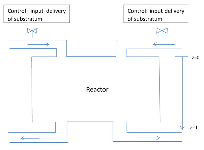
Figure 1: Regulation of the concentration flux of the substratum at the upper bottom of the reactor

Anther example the energy exchange problem between a casting plasma on a plane target which is perpendicular to the direction of the flow sub-diffusion process from measurements carried out by internal thermocouples ([Zerrik, Bourray $\&$ Badraoui, 2000]). For richer background on gradient modeling, we refer the reader to [Cortés, Schaft $\&$ Crouch, 2005] and [Kessell, 2012]. To the best of our knowledge, no results are available on this topic and we hope that the results obtained here could provide some insights into the control theory analysis of the fractional order diffusion systems and be useful in real-life applications.

The rest contents of the present paper are structured as follows. The problem studied and some preliminaries are introduced in the next section and in Section $\ref{section3},$ we focus on the characteristic of the strategic sensors. An approach which enables us to reconstruct the initial gradient vector of the system under consideration in the considered subregion is addressed in Section 4. Several application examples are worked out in the end for illustrations.

2 Problem formulation and preliminaries

In this section, we formulate the regional gradient observability problems for the Riemann-Liouville time fractional order diffusion system and then introduce some preliminary results to be used thereafter.

2.1 Problem formulation

Let $\Omega$ be a connected, open bounded subset of $\mathbf{R}^{n}$ with Lipschitz continuous boundary $\partial\Omega$ and consider the following abstract time fractional diffusion process:

$$\left.\begin{array}[]{l}{}_{0}D^{\alpha}_{t}y(t)=Ay(t),~{}~{}t\in[0,b],~{}0<\alpha\leq 1,\\ \lim\limits_{t\to 0^{+}}{}_{0}I^{1-\alpha}_{t}y(t)=y_{0}\mbox{ supposed to be unknown,}\end{array}\right\}$$ (1)

where $A$ generates a strongly continuous semigroup $\{\Phi(t)\}_{t\geq 0}$ on the Hilbert space $Y:=L^{2}(\Omega)$, $-A$ is a uniformly elliptic operator, $y\in L^{2}(0,b;Y)$, ${}_{0}D^{\alpha}_{t}$ and ${}_{0}I^{\alpha}_{t}$ denote the Riemann-Liouville fractional order derivative and integral with respect to time $t$, respectively, given by ([Kilbas, Srivastava $\&$ Trujillo, 2006] and [Podlubny, 1999])

$${}_{0}D_{t}^{\alpha}y(t) = \frac{\partial}{\partial t}{}_{0}I_{t}^{1-\alpha}y(t),~{}0<\alpha\leq 1~{}~{}\mbox{ and }$$

$${}_{0}I^{\alpha}_{t}y(t) = \frac{1}{\Gamma(\alpha)}\int^{t}_{0}{(t-s)^{\alpha-1}y(s)ds},~{}\alpha>0.$$

The measurements (possibly unbounded) are given depending on the number and the structure of the sensors with dense domain in $L^{2}(0,b;Y)$ and range in $L^{2}(0,b;\mathbf{R}^{p})$ as follows:

$$z(t)=Cy(t),$$ (2)

where $p\in\mathbf{N}$ is the finite number of sensors.

Let $y_{0}\in H_{0}^{1}(\Omega)$ and both the initial vector $y_{0}$ and its gradient are supposed to be unknown. The system $(\ref{problem})$ admits a unique mild solution given by ([Ge, Chen $\&$ Kou, 2016] and [Liu $\&$ Li, 2015]):

$$y(t)=S_{\alpha}(t)y_{0},~{}~{}t\in[0,b],$$ (3)

where $S_{\alpha}(t)=\alpha t^{\alpha-1}\int_{0}^{\infty}{\theta\phi_{\alpha}(\theta)\Phi(t^{\alpha}\theta)}d\theta,$ $\{\Phi(t)\}_{t\geq 0}$ is the strongly continuous semigroup generated by $A$, $\phi_{\alpha}(\theta)=\frac{1}{\alpha}\theta^{-1-\frac{1}{\alpha}}\psi_{\alpha}(\theta^{-\frac{1}{\alpha}})$ and $\psi_{\alpha}$ is a probability density function defined by $(\theta\in(0,\infty))$

$$\psi_{\alpha}(\theta)=\frac{1}{\pi}\sum\limits_{n=1}^{\infty}{(-1)^{n-1}\theta^{-\alpha n-1}\frac{\Gamma(n\alpha+1)}{n!}\sin(n\pi\alpha)}$$ (4)

satisfying ([Mainardi, Paradisi $\&$ Gorenflo, 2007])

$$\int_{0}^{\infty}{\psi_{\alpha}(\theta)}d\theta=1\mbox{ and }\int_{0}^{\infty}{\theta^{\nu}\phi_{\alpha}(\theta)}d\theta=\frac{\Gamma(1+\nu)}{\Gamma(1+\alpha\nu)},\nu\geq 0.$$

2.2 Definitions and characterizations

Let $\omega\subseteq\Omega$ be a given region of positive Lebesgue measure and let

$$y_{0}=\left\{\begin{array}[]{l}y_{0}^{1},~{}\omega~{}\mbox{ to be estimated,}\\ y_{0}^{2},~{}\Omega\backslash\omega~{}\mbox{ undesired.}\end{array}\right.$$ (5)

Then the regional gradient observability problem is concerned with the directly reconstruction of the initial gradient vector $\nabla y_{0}^{1}$ in $\omega$. Consider the following two restriction mappings

$$p_{\omega}:~{}\left\{\begin{array}[]{l}\left(L^{2}(\Omega)\right)^{n}\to\left(L^{2}(\omega)\right)^{n}_{,}\\ ~{}\xi\to\xi|_{\omega}\end{array}\right.p_{1\omega}:~{}\left\{\begin{array}[]{l}L^{2}(\Omega)\to L^{2}(\omega),\\ ~{}y\to y|_{\omega}.\end{array}\right.$$

Their adjoint operators are, respectively, denoted by

$$p_{\omega}^{*}:~{}\left\{\begin{array}[]{l}\left(L^{2}(\omega)\right)^{n}\to\left(L^{2}(\Omega)\right)^{n},\\ ~{}\xi\to p_{\omega}^{*}\xi=\left\{\begin{array}[]{l}\xi,~{}~{}x\in\omega,\\ 0,~{}~{}x\in\Omega\backslash\omega\end{array}\right.\end{array}\right.$$ (7)

and

$$p_{1\omega}^{*}:~{}\left\{\begin{array}[]{l}L^{2}(\omega)\to L^{2}(\Omega),\\ ~{}y\to p_{1\omega}^{*}y=\left\{\begin{array}[]{l}y,~{}~{}x\in\omega,\\ 0,~{}~{}x\in\Omega\backslash\omega.\end{array}\right.\end{array}\right.$$ (8)

Moreover, by Eq. $(\ref{solution})$, the output function $(\ref{outputfunction})$ gives

$$z(t)=CS_{\alpha}(t)y_{0}=K(t)y_{0},$$ (9)

where $K:H_{0}^{1}(\Omega)\to L^{2}(0,b;\mathbf{R}^{p})$. To obtain the adjoint operator of $K$, we have
Case 1. $C$ is bounded (e.g. zone sensors)
Denote the adjoint operator of $C$ and $S_{\alpha}$ by $C^{*}$ and $S_{\alpha}^{*}$, respectively. Since $S_{\alpha}$ is a bounded operator ([Zhou $\&$ Jiao, 2010]), we get that the adjoint operator of $K$ can be given by

$$K^{*}:~{}\left\{\begin{array}[]{l}L^{2}(0,b;\mathbf{R}^{p})\to Y,\\ ~{}z\to\int_{0}^{b}{S^{*}_{\alpha}(s)C^{*}z(s)}ds.\end{array}\right.$$ (10)

Case 2. $C$ is unbounded (e.g. pointwise sensors)
Note that $C$ is densely defined, then $C^{*}$ exists. To state our results, the following two assumptions are needed:

$(A_{1})$ $CS_{\alpha}(t)$ can be extended to a bounded linear operator $\overline{CS_{\alpha}(t)}$ in $\mathcal{L}\left(Y,L^{2}(0,b;\mathbf{R}^{p})\right)$;
$(A_{2})$ $(CS_{\alpha})^{*}$ exists and $(CS_{\alpha})^{*}=S_{\alpha}^{*}C^{*}$.

Extend $K$ by $K(t)y_{0}=\overline{CS_{\alpha}(t)}y_{0},$ one has $K\in\mathcal{L}\left(Y,L^{2}(0,b;\mathbf{R}^{p})\right).$ Based on the Hahn-Banach theorem, similar to the argument in [Pritchard $\&$ Wirth, 1978], it is possible to derive the duality theorems as in [Curtain $\&$ Zwart, 2012] and [Dolecki $\&$ Russell, 1977] with the above two assumptions. Then the adjoint operator of $K$ can be defined as

$$K^{*}:~{}\left\{\begin{array}[]{l}D(K^{*})\subseteq L^{2}(0,b;\mathbf{R}^{p})\to Y,\\ ~{}z\to\int_{0}^{b}{S^{*}_{\alpha}(s)C^{*}z(s)}ds.\end{array}\right.$$ (11)

Let $\nabla:H_{0}^{1}(\Omega)\to\left(L^{2}(\Omega)\right)^{n}$ be an operator defined by

$$y\to\nabla y(x):=\left(\frac{\partial y}{\partial x_{1}},\frac{\partial y}{\partial x_{2}},\cdots,\frac{\partial y}{\partial x_{n}}\right).$$ (12)

We see that the adjoint of the gradient operating on a connected, open bounded subset $\Omega$ with a Lipschitz continuous boundary $\partial\Omega$ is minus the divergence operator, i.e., $\nabla^{*}:\left(L^{2}(\Omega)\right)^{n}\to H^{-1}(\Omega)$ is given by ([Kurula $\&$ Zwart, 2012])

$$\xi\to\nabla^{*}\xi:=v,$$ (13)

where $v$ solves the following Dirichlet problem

$$\left\{\begin{array}[]{l}v=-\mbox{div}(\xi)~{}\mbox{ in }\Omega,\\ ~{}v=0~{}\mbox{ on }\partial\Omega.\end{array}\right.$$ (14)

Similar to the discussion in [Curtain $\&$ Zwart, 2012]; [Dolecki $\&$ Russell, 1977] and [Pritchard $\&$ Wirth, 1978], it follows that the necessary and sufficient condition for the regional weak observability of the system described by $(\ref{problem})$ and $(\ref{outputfunction})$ in $\omega$ at time $b$ is that $Ker\left(Kp_{1\omega}^{*}\right)=\{0\}\subseteq L^{2}(\Omega)$ and we see the following definition.

Definition 1.

The system $(\ref{problem})$ with output function $(\ref{outputfunction})$ is said to be regional weak gradient observability in $\omega$ at time $b$ if and only if

$$Ker\left(K\nabla^{*}p_{\omega}^{*}\right)=\{(0,0,\cdots,0)\}\subseteq\left(L^{2}(\Omega)\right)^{n}.$$ (15)

Proposition 2.

There is an equivalence among the following properties:

$\left<1\right>$ The system $(\ref{problem})$ is regional weak gradient observability in $\omega$ at time $b$;
$\left<2\right>$ $\overline{Im\left(p_{\omega}\nabla K^{*}\right)}=\left(L^{2}(\omega)\right)^{n};$
$\left<3\right>$ The operator $p_{\omega}\nabla K^{*}K\nabla^{*}p^{*}_{\omega}$ is positive definite.

Proof. By Definition 1, it is obvious to know that $\left<1\right>\Leftrightarrow\left<2\right>.$ As for $\left<2\right>\Leftrightarrow\left<3\right>,$ in fact, we have

$$\overline{Im\left(p_{\omega}\nabla K^{*}\right)}=\left(L^{2}(\omega)\right)^{n} \Leftrightarrow (p_{\omega}\nabla K^{*}z,y)=0,~{}\forall z\in Z\Rightarrow$$

$$y=(0,0,\cdots,0)\in\left(L^{2}(\Omega)\right)^{n}.$$

Let $z=K\nabla^{*}p_{\omega}^{*}y\in Z$, which then allows us to complete the proof.

Remark 3.

$\left.1\right)$ When $\alpha=1$, the system $(\ref{problem})$ is deduced to the normal diffusion process as considered in [Zerrik $\&$ Bourray, 2003b], which is a particular case of our results.

$\left.2\right)$ A system which is gradient observable on $\omega$ is gradient observable on $\omega_{1}$ for every $\omega_{1}\subseteq\omega.$ Moreover, the Definition 1 is also valid for the case when $\omega=\Omega$ and there exist systems that are not gradient observable but regionally gradient observable. This can be illustrated by the following example.

2.3 An example

Let $\Omega=[0,1]\times[0,1]\subseteq\mathbf{R}^{2}$ and consider the following time fractional order diffusion system of order $\alpha\in(0,1]$.

$$\left\{\begin{array}[]{l}_{0}D^{\alpha}_{t}y(x_{1},x_{2},t)=\left(\frac{\partial^{2}}{\partial x_{1}^{2}}+\frac{\partial^{2}}{\partial x_{2}^{2}}\right)y(x_{1},x_{2},t)\mbox{ in }\Omega\times[0,b],\\ y(\xi,\eta,t)=0~{}\mbox{ on }\partial\Omega\times[0,b],\\ \lim\limits_{t\to 0^{+}}{}_{0}I^{1-\alpha}_{t}y(x_{1},x_{2},t)=y_{0}(x_{1},x_{2})~{}\mbox{ in }\Omega\end{array}\right.$$ (19)

with the output functions

$$z(t)=Cy(t)=\int_{0}^{1}\int_{0}^{1}{f(x_{1},x_{2})y(x_{1},x_{2},t)}dx_{1}dx_{2},$$ (20)

where $f(x_{1},x_{2})=\delta(x_{1}-1/2)\sin(\pi x_{2})$ and $\delta(x)$ is the Dirac delta function on the real number line that is zero everywhere except at zero.

According to the problem $(\ref{problem})$, $A=\frac{\partial^{2}}{\partial x_{1}^{2}}+\frac{\partial^{2}}{\partial x_{2}^{2}}$. Then the eigenvalue, eigenvector and the semigroup $\Phi(t)$ on $Y$ generated by $A$ are respectively $\lambda_{ij}=-(i^{2}+j^{2})\pi^{2}$, $\xi_{ij}(x_{1},x_{2})=2\sin(i\pi x_{1})\sin(j\pi x_{2})$ and $\Phi(t)y(x)=\sum\limits_{i,j=1}^{\infty}{\exp(\lambda_{ij}t)(y,\xi_{ij})\xi_{ij}}(x).$ Moreover, one has ([Ge, Chen $\&$ Kou, 2016])

$$S_{\alpha}(t)y_{0}(x)=\sum\limits_{i,j=1}^{\infty}t^{\alpha-1}E_{\alpha,\alpha}(\lambda_{ij}t^{\alpha})(y_{0},\xi_{ij})\xi_{ij}(x),$$

where $E_{\alpha,\beta}(z):=\sum\limits_{i=0}^{\infty}{\frac{z^{i}}{\Gamma(\alpha i+\beta)}},$ $\mathbf{Re}{\kern 2.0pt}\alpha>0,~{}\beta,z\in\mathbf{C}$ is the generalized Mittag-Leffler function in two parameters.

Next, we show that there is a gradient vector $g$, which is not gradient observable in the whole domain but gradient observable in a subregion $\omega\subseteq\Omega$.

Let $g=\frac{1}{\pi}(\cos(\pi x_{1})\sin(3\pi x_{2}),3\sin(\pi x_{1})\cos(3\pi x_{2}))\in\left(L^{2}(\Omega)\right)^{2}$. By Eq. $(\ref{2.10})$, we obtain that $\nabla^{*}g=10\sin(\pi x_{1})\sin(3\pi x_{2})$, then

$$K\nabla^{*}g = CS_{\alpha}(t)\nabla^{*}g$$

$$= 40\sum\limits_{i,j=1}^{\infty}t^{\alpha-1}E_{\alpha,\alpha}(\lambda_{ij}t^{\alpha})\int_{0}^{1}{\sin(\pi x_{1})\sin(i\pi x_{1})}dx_{1}$$

$$\times\int_{0}^{1}{\sin(3\pi x_{2})\sin(j\pi x_{2})}dx_{2}$$

$$\times\sin\left(\frac{i\pi}{2}\right)\int_{0}^{1}{\sin(\pi x_{2})\sin(j\pi x_{2})}dx_{2}$$

$$= 0.$$

However, let $\omega=[0,1]\times[0,1/6],$ we see that

$$K\nabla^{*}p^{*}_{\omega}p_{\omega}g = CS_{\alpha}(t)\nabla^{*}p^{*}_{\omega}p_{\omega}g$$

$$= 40\sum\limits_{i,j=1}^{\infty}t^{\alpha-1}E_{\alpha,\alpha}(\lambda_{ij}t^{\alpha})\int_{0}^{1}{\sin(\pi x_{1})\sin(i\pi x_{1})}dx_{1}$$

$$\times\int_{0}^{1/6}{\sin(3\pi x_{2})\sin(j\pi x_{2})}dx_{2}$$

$$\times\sin\left(\frac{i\pi}{2}\right)\int_{0}^{1}{\sin(\pi x_{2})\sin(j\pi x_{2})}dx_{2}$$

$$= \frac{5\sqrt{3}t^{\alpha-1}E_{\alpha,\alpha}(-2\pi^{2}t^{\alpha})}{8\pi}\neq 0,$$

which means that $g$ is gradient observable in $\omega.$

The following two lemmas play a significant role to obtain our results.

Lemma 4.

([Podlubny $\&$ Chen, 2007]) For any $t\in[a,b]$, $\alpha\in(0,1)$, the following formula holds

$$\int_{a}^{b}{f(t){}_{a}D_{t}^{\alpha}g(t)}dt=\left[f(t){}_{a}I_{t}^{1-\alpha}g(t)\right]_{t=a}^{t=b}-\int_{a}^{b}{g(t){}_{t}^{C}D_{b}^{\alpha}f(t)}dt.$$

Lemma 5.

([Dacorogna, 2007]) Let $\Omega\subseteq\mathbf{R}^{n}$ be an open set and $C_{0}^{\infty}(\Omega)$ be the class of infinitely differentiable functions on $\Omega$ with compact support in $\Omega$ and $u\in L^{1}_{loc}(\Omega)$ be such that

$$~{}~{}~{}~{}~{}~{}~{}~{}~{}~{}~{}~{}~{}~{}\int_{\Omega}u(x)\psi(x)dx=0,~{}~{}~{}\forall\psi\in C_{0}^{\infty}(\Omega).$$ (21)

Then $u=0$ almost everywhere in $\Omega.$

3 Regional strategic sensors

This section is devoted to addressing the characteristic of sensors when the studied system is regionally gradient observable in a given subregion of the whole domain.

Firstly, we recall that a sensor can be defined by a couple $(D,f)$ where $D\subseteq\Omega$ is the support of the sensor and $f$ is its spatial distribution. For example, if $D=\{\sigma\}$ with $\sigma\in\bar{\Omega}$ and $f=\delta_{\sigma},$ where $\delta_{\sigma}=\delta(\cdot-\sigma)$ is the Dirac delta function in $\omega$ at time $b$ that is zero everywhere except at $\sigma,$ the sensor is called pointwise sensor. In this case the operator $C$ is unbounded and the output function can be written as $z(t)=y(\sigma,t).$ It is called zone sensor when $D\subseteq\bar{\Omega}$ and $f\in Y$. The output function is bounded and can be defined as follows: $z(t)=\int_{D}{y(x,t)f(x)}dx.$ For more information on the structure characteristic and properties of sensors and actuators, we refer the reader to ([El Jai, 1991], [El Jai $\&$ Pritchard, 1988], [Zerrik $\&$ Bourray, 2003b]) and the references cited therein.

Next, to state our results, it is supposed that the measurements are made by $p$ sensors $(D_{i},f_{i})_{1\leq i\leq p}$, where $D_{i}\subseteq\Omega$ and $f_{i}\in L^{2}(\Omega)$, $i=1,2,\cdots,p.$ Then $(\ref{problem})$ can be rewritten as

$$\left\{\begin{array}[]{l}{}_{0}D^{\alpha}_{t}y(x,t)=Ay(x,t)~{}\mbox{ in }\Omega\times[0,b],\\ y(\eta,t)=0~{}~{}\mbox{ on }\partial\Omega\times[0,b],\\ \lim\limits_{t\to 0^{+}}{}_{0}I^{1-\alpha}_{t}y(x,t)=y_{0}(x)~{}\mbox{ in }\Omega\end{array}\right.$$ (22)

with the measurements

$$z(t)=Cy(x,t)=\left(z_{1}(t),z_{2}(t),\cdots,z_{p}(t)\right)^{T}\in\mathbf{R}^{p},$$ (23)

where $z_{i}(t)=\left(y(\cdot,t),f_{i}\right)_{L^{2}(D_{i})}$.

Moreover, since the operator $-A$ is a uniformly elliptic operator, for any $y_{i}\in L^{2}(0,b;Y),$ $i=1,2$, $A$ satisfies

$$\int_{Q}{y_{1}(x,t)Ay_{2}(x,t)}dtdx-\int_{Q}{y_{2}(x,t)A^{*}y_{1}(x,t)}dtdx$$

$$=\int_{\partial\Omega\times[0,b]}{\left[y_{1}(\eta,t)\frac{\partial y_{2}(\eta,t)}{\partial v_{A}}-y_{2}(\eta,t)\frac{\partial y_{2}(\eta,t)}{\partial v_{A^{*}}}\right]}dtd\eta,$$

where $A^{*}$ is the adjoint operator of $A$. Moreover, by [Courant $\&$ Hilbert, 1966], there exists a sequence $(\lambda_{j},\xi_{jk}):k=1,2,\cdots,r_{j}$, $j=1,\cdots$ such that

$1)$ Each $\lambda_{j}$ $(j=1,2,\cdots)$ is the eigenvalue of the operator $A$ with multiplicities $r_{j}$ and

$$0>\lambda_{1}>\lambda_{2}>\cdots>\lambda_{j}>\cdots,~{}~{}\lim\limits_{j\to\infty}\lambda_{j}=-\infty.$$

$2)$ For each $j=1,2,\cdots$, $\xi_{jk}~{}(k=1,2,\cdots,r_{j})$ is the orthonormal eigenfunction corresponding to $\lambda_{j}$, i.e.,

$$(\xi_{jk_{m}},\xi_{jk_{n}})=\left\{\begin{array}[]{l}1,~{}~{}k_{m}=k_{n},\\ 0,~{}~{}k_{m}\neq k_{n},\end{array}\right.$$

where $1\leq k_{m},k_{n}\leq r_{j},$ $k_{m},k_{n}\in\mathbf{N}$ and $(\cdot,\cdot)$ is the inner product of space $Y$. Then it follows that the strongly continuous semigroup $\{\Phi(t)\}_{t\geq 0}$ on $Y$ generated by $A$ can be expressed as

$$\Phi(t)y(x)=\sum\limits_{j=1}^{\infty}{\sum\limits_{k=1}^{r_{j}}{\exp(\lambda_{j}t)(y,\xi_{jk})\xi_{jk}(x)}},~{}~{}x\in\Omega,$$ (24)

the sequence $\{\xi_{jk},k=1,2,\cdots,r_{j},j=1,2,\cdots\}$ is an orthonormal basis in $Y$ and for any $y_{*}(x)\in Y$, it can be expressed as $y_{*}(x)=\sum\limits_{j=1}^{\infty}{\sum\limits_{k=1}^{r_{j}}(y_{*},\xi_{jk})\xi_{jk}(x)}.$

Definition 6.

A sensor (or a suite of sensors) is said to be gradient $\omega-$strategic if the observed system is regionally gradient observable in $\omega$.

Lemma 7.

For any $z(t)=\left(z_{1}(t),z_{2}(t),\cdots,z_{p}(t)\right)^{T}\in\mathbf{R}^{p}$ with $z_{i}\in L^{2}(0,b),$ $i=1,2,\cdots,p$, suppose that $e(x,t)$ satisfies the following system

$$\left\{\begin{array}[]{l}{}^{C}_{t}D^{\alpha}_{b}e(x,t)=-A^{*}e(x,t)+\sum\limits_{i=1}^{p}{p_{D_{i}}f_{i}(x)z_{i}(t)}\\ {\kern 150.0pt}\mbox{ in }\Omega\times[0,b],\\ e(\eta,t)=0~{}~{}\mbox{ on }\partial\Omega\times[0,b],\\ e(x,b)=0~{}~{}\mbox{ in }\Omega,\end{array}\right.$$ (25)

where $A^{*}$ is the adjoint operator of $A$ and ${}_{t}^{C}D^{\alpha}_{b}$ denotes the right-sided Caputo fractional order derivative with respect to time $t$ of order $\alpha\in(0,1]$ given by ([Kilbas, Srivastava $\&$ Trujillo, 2006]; [Podlubny, 1999] and [Podlubny $\&$ Chen, 2007])

$${}_{t}^{C}D_{b}^{\alpha}e(x,t)=\frac{-1}{\Gamma(1-\alpha)}\int_{t}^{b}{(\tau-t)^{-\alpha}\frac{\partial}{\partial\tau}e(x,\tau)}d\tau.$$ (26)

Then we obtain that $K^{*}z=-e(x,0).$

Proof. Replacing $t$ in ${}_{t}^{C}D_{b}^{\alpha}e(x,t)$ by $b-t$, we have

$$\begin{array}[]{l}~{}~{}~{}~{}{}^{C}_{(b-t)}D^{\alpha}_{b}e(x,b-t)\\ =\frac{-1}{\Gamma(1-\alpha)}\int_{b-t}^{b}{(\tau-b+t)^{-\alpha}\frac{\partial}{\partial\tau}e(x,\tau)}d\tau\\ =\frac{-1}{\Gamma(1-\alpha)}\int_{0}^{t}{(t-s)^{-\alpha}\left[-\frac{\partial}{\partial s}e(x,b-s)\right]}ds\\ =-{}^{C}_{0}D^{\alpha}_{t}e(x,b-t).\end{array}$$

Then the system $(\ref{efunction})$ is equivalent to

$$\left\{\begin{array}[]{l}{}^{C}_{0}D^{\alpha}_{t}e(x,b-t)=A^{*}e(x,b-t){}\\ {\kern 41.0pt}-\sum\limits_{i=1}^{p}{p_{D_{i}}f_{i}(x)z_{i}(b-t)}\mbox{ in }\Omega\times[0,b],\\ e(\eta,b-t)=0~{}~{}\mbox{ on }\partial\Omega\times[0,b],\\ e(x,b-0)=0~{}~{}\mbox{ in }\Omega.\end{array}\right.$$ (28)

Similar to the argument in [Ge, Chen $\&$ Kou, 2016] and [Sakamoto $\&$ Yamamoto, 2011], the mild solution of $(\ref{efunction})$ can be given by

$$e(x,t)=-\int_{0}^{b-t}{S_{\alpha}^{*}(b-t-s)\sum\limits_{i=1}^{p}{p_{D_{i}}f_{i}(x)z_{i}(b-s)}}ds.$$

On the other hand, it follows from the definition of the adjoint operator of $K$ that

$$K^{*}z=\int_{0}^{b}{S^{*}_{\alpha}(s)C^{*}z(s)}ds=\int_{0}^{b}{S^{*}_{\alpha}(s)\sum\limits_{i=1}^{p}{p_{D_{i}}f_{i}(x)z_{i}(s)}}ds.$$

This allows us to complete the proof.

Theorem 8.

For any $j=1,2,\cdots$, $s=1,2,\cdots,n$, given arbitrary $b>0$, define the following $p\times r_{j}$ matrices $G_{j}^{s}$

$$G_{j}^{s}=\left[{\begin{array}[]{*{20}{c}}{\xi_{j1}^{1s}}&{\xi_{j2}^{1s}}&{\cdots}&{\xi_{jr_{j}}^{1s}}\\ {\xi_{j1}^{2s}}&{\xi_{j2}^{2s}}&{\cdots}&{\xi_{jr_{j}}^{2s}}\\ {\vdots}&{\vdots}&{\vdots}&{\vdots}\\ {\xi_{j1}^{ps}}&{\xi_{j2}^{ps}}&{\cdots}&{\xi_{jr_{j}}^{ps}}\end{array}}\right]_{p\times r_{j}},$$ (29)

where $\xi_{jk}^{is}=\left(\frac{\partial\xi_{jk}}{\partial x_{s}},f_{i}\right)_{L^{2}(D_{i})}$, $i=1,2,\dots,p$ and $k=1,2,\cdots,r_{j}$. For all $j=1,2,\cdots,$ let $y_{jks}=(p_{1\omega}^{*}y_{s},\xi_{jk})$ and $y_{js}=(y_{j1s},y_{j2s},\cdots,y_{jr_{j}s})^{T}\in\mathbf{R}^{r_{j}}$. Then the necessary and sufficient condition for the gradient $\omega-$strategic of the sensors $(D_{i},f_{i})_{1\leq i\leq p}$ is that

$$\sum\limits_{s=1}^{n}G_{j}^{s}y_{js}=\mathbf{0}_{p}:=(0,0,\cdots,0)^{T}\in\mathbf{R}^{p}~{}\Rightarrow{\kern 60.0pt}$$

$${\kern 80.0pt}y=\mathbf{0}_{n}:=(0,\cdots,0)^{T}\in\left(L^{2}(\omega)\right)^{n}.$$

In particular, when $n=1,$ the sensors $(D_{i},f_{i})_{1\leq i\leq p}$ is gradient $\omega-$strategic if and only if

$$(1)~{}p\geq r=\max\{r_{j}\};$$

$$(2)~{}rank~{}G_{j}^{1}=r_{j}\mbox{ for all }j=1,2,\cdots.$$

$\mathbf{Proof.}$ Given arbitrary $b>0$, by Definition 1, the sensors $(D_{i},f_{i})_{1\leq i\leq p}$ are gradient $\omega-$strategic if and only if for any $z\in L^{2}(0,b;\mathbf{R}^{p})$,

$$\left\{y\in\left(L^{2}(\omega)\right)^{n}|\left(p_{\omega}\nabla K^{*}z,y\right)_{\left(L^{2}(\omega)\right)^{n}}=0\right\}\Rightarrow y=\mathbf{0}_{n},$$

where $y=(y_{1},y_{2},\cdots,y_{n})$ with $y_{s}\in L^{2}(\omega)$.

Let $x=(x_{1},x_{2},\cdots,x_{n})\in\Omega$. By Lemma $\ref{lemma3.1},$ we have

$$\left(p_{\omega}\nabla K^{*}z,y\right)_{\left(L^{2}(\omega)\right)^{n}} = \left(\nabla K^{*}z,p_{\omega}^{*}y\right)_{\left(L^{2}(\Omega)\right)^{n}}$$

$$= \sum\limits_{s=1}^{n}\left(\frac{\partial(K^{*}z)}{\partial x_{s}},p_{1\omega}^{*}y_{s}\right)_{L^{2}(\Omega)}$$

$$= \sum\limits_{s=1}^{n}\left(\frac{\partial\left[-e(x,0)\right]}{\partial x_{s}},p_{1\omega}^{*}y_{s}\right)_{L^{2}(\Omega)},$$

where $e$ is the solution of the system $(\ref{efunction})$.

Next, we explore the exact expression of $\left(p_{\omega}\nabla K^{*}z,y\right)_{\left(L^{2}(\omega)\right)^{n}}.$ Consider the following problem

$$\left\{\begin{array}[]{l}{}_{0}D^{\alpha}_{t}\rho(x,t)=A\rho(x,t)~{}\mbox{in }\Omega\times[0,b],\\ \rho(\eta,t)=0~{}~{}\mbox{on }\partial\Omega\times[0,b],\\ \lim\limits_{t\to 0^{+}}{}_{0}I^{1-\alpha}_{t}\rho(x,t)=p_{1\omega}^{*}y_{s}(x){\kern 5.0pt}~{}\mbox{in }\Omega,\end{array}\right.$$ (30)

where $s=1,2,\cdots,n$ and the unique mild solution of system $(\ref{adjointproblem})$ can be given by ([Sakamoto $\&$ Yamamoto, 2011])

$$\begin{array}[]{l}\rho(x,t)=\sum\limits_{j=1}^{\infty}\sum\limits_{k=1}^{r_{j}}E_{\alpha,\alpha}(\lambda_{j}t^{\alpha})\left(p_{1\omega}^{*}y_{s},\xi_{jk}\right)\xi_{jk}(x).\end{array}$$ (32)

Multiplying both sides of $(\ref{efunction})$ with $\frac{\partial\rho(x,t)}{\partial x_{s}}$ and integrating the results over the domain $Q:=\Omega\times[0,b]$,

$$\begin{array}[]{l}\int_{Q}{\left[{}_{t}^{C}D^{\alpha}_{b}e(x,t)\right]\frac{\partial\rho(x,t)}{\partial x_{s}}}dtdx\\ =-\int_{Q}{A^{*}e(x,t)\frac{\partial\rho(x,t)}{\partial x_{s}}}dtdx\\ {\kern 8.0pt}+\int_{0}^{b}\int_{\Omega}{\sum\limits_{i=1}^{p}{p_{D_{i}}f_{i}(x)z_{i}(t)}\frac{\partial\rho(x,t)}{\partial x_{s}}}dxdt.\end{array}$$

Consider the fractional integration by parts $(\ref{derivativeparts})$ in Lemma 4, one has

$$\begin{array}[]{l}\int_{Q}{\left[{}_{t}^{C}D^{\alpha}_{b}e(x,t)\right]\frac{\partial\rho(x,t)}{\partial x_{s}}}dtdx\\ =-\int_{\Omega}{\left[\lim\limits_{t\to 0^{+}}{}_{0}I^{1-\alpha}_{t}\rho(x,t)\right]\frac{\partial e(x,0)}{\partial x_{s}}}dx\\ {\kern 8.0pt}-\int_{Q}{e(x,t)\left[{}_{0}D^{\alpha}_{t}\frac{\partial\rho(x,t)}{\partial x_{s}}\right]}dtdx.\end{array}$$

Then the boundary condition gives

$$\begin{array}[]{l}\int_{\Omega}{\frac{\partial\left[-e(x,0)\right]}{\partial x_{s}}\left[\lim\limits_{t\to 0^{+}}{}_{0}I^{1-\alpha}_{t}e(x,t)\right]}dx\\ {\color[rgb]{1.00,0.00,0.00}=}\int_{0}^{b}\int_{\Omega}{\sum\limits_{i=1}^{p}{p_{D_{i}}f_{i}(x)z_{i}(t)}\frac{\partial\rho(x,t)}{\partial x_{s}}}dxdt,~{}s=1,2,\cdots,n.\end{array}$$

Thus, we have

$$\left(p_{\omega}\nabla K^{*}z,y\right)_{\left(L^{2}(\omega)\right)^{n}}$$

$$= \sum\limits_{s=1}^{n}\left(\frac{\partial\left[-e(x,0)\right]}{\partial x_{s}},p_{1\omega}^{*}y_{s}\right)_{L^{2}(\Omega)}$$

$$= \sum\limits_{s=1}^{n}\left(\frac{\partial\left[-e(x,0)\right]}{\partial x_{s}},\left[\lim\limits_{t\to 0^{+}}{}_{0}I^{1-\alpha}_{t}e(x,t)\right]\right)_{L^{2}(\Omega)}$$

$$= \sum\limits_{s=1}^{n}\sum\limits_{j=1}^{\infty}\sum\limits_{k=1}^{r_{j}}\sum\limits_{i=1}^{p}\int_{0}^{b}{E_{\alpha,\alpha}(\lambda_{j}\tau^{\alpha})z_{i}(\tau)}d\tau\left(\frac{\partial\xi_{jk}}{\partial x_{s}},p_{D_{i}}f_{i}\right)y_{jks}.$$

By Lemma 5, since $z\in L^{2}(0,b;\mathbf{R}^{p})$ is arbitrary, we see that the system $(\ref{problem})$ is regionally gradient observable in $\omega$ at time $b$ if and only if

$$\sum\limits_{s=1}^{n}\sum\limits_{j=1}^{\infty}E_{\alpha,\alpha}(\lambda_{j}t^{\alpha})\sum\limits_{i=1}^{p}\sum\limits_{k=1}^{r_{j}}\xi_{jk}^{is}y_{jks}=\mathbf{0}_{p}\Rightarrow y=\mathbf{0}_{n},$$ (36)

i.e., for any $y=(y_{1},y_{2},\cdots,y_{n})\in\left(L^{2}(\Omega)\right)^{n}$, one has

$$\sum\limits_{j=1}^{\infty}{E_{\alpha,\alpha}(\lambda_{j}t^{\alpha})}\sum\limits_{s=1}^{n}G_{j}^{s}y_{js}=\mathbf{0}_{p}~{}\Rightarrow y=\mathbf{0}_{n},$$ (37)

where $y_{js}=(y_{j1s},y_{j2s},\cdots,y_{jr_{j}s})^{T}$ is a vector in $\mathbf{R}^{r_{j}}$.

Finally, since $E_{\alpha,\alpha}(\lambda_{j}t^{\alpha})>0$ for all $t\geq 0$, $j=1,2,\cdots,$ we then show our proof by using the Reductio and Absurdum.

$(a)$ Necessity. If $p\geq r=\max\{r_{j}\}$ and $rank~{}G_{j}^{s}<r_{j}\mbox{ for some }j=1,2,\cdots$ and $s=1,2,\cdots,p,$ there exists a nonzero element $\tilde{y}\in\left(L^{2}(\omega)\right)^{n}$ with $\tilde{y}_{js}=\left(\tilde{y}_{j1s},\tilde{y}_{j2s},\cdots,\tilde{y}_{jr_{j}s}\right)^{T}\in\mathbf{R}^{r_{j}}$ such that $G_{j}^{s}\tilde{y}_{js}=\mathbf{0}_{p}.$ Then we can find a nonzero vector $\tilde{y}\in\left(L^{2}(\omega)\right)^{n}$ satisfying $\sum\limits_{j=1}^{\infty}{E_{\alpha,\alpha}(\lambda_{j}t^{\alpha})}\sum\limits_{s=1}^{n}G_{j}^{s}\tilde{y}_{js}=\mathbf{0}_{p}.$ This means that the sensors $(D_{i},f_{i})_{1\leq i\leq p}$ are not $\omega-$strategic.

$(b)$ Sufficiency. On the contrary, if the sensors $(D_{i},f_{i})_{1\leq i\leq p}$ are not $\omega-$strategic, i.e., $\overline{Im\left(p_{\omega}\nabla K^{*}\right)}\neq\left(L^{2}(\omega)\right)^{n}.$ Then there exists a nonzero element $y_{j^{*}s}\in\mathbf{R}^{r_{j}}$ such that $\sum\limits_{s=1}^{n}G_{j^{*}}^{s}y_{j^{*}s}=\mathbf{0}_{p}.$ This allows us to complete the first conclusion of the theorem.

In particular, when $n=s=1,$ similar to the argument in $(a)$, if $p\geq r=\max\{r_{j}\}$ and $rank~{}G_{j}^{1}<r_{j}\mbox{ for some }j=1,2,\cdots$, there exists a nonzero vector $\tilde{y}\in\left(L^{2}(\omega)\right)^{n}$ satisfying $\sum\limits_{j=1}^{\infty}{E_{\alpha,\alpha}(\lambda_{j}t^{\alpha})}G_{j}^{1}\tilde{y}_{js}=\mathbf{0}_{p}.$ Then the sensors $(D_{i},f_{i})_{1\leq i\leq p}$ are not $\omega-$strategic.

Moreover, if the sensors $(D_{i},f_{i})_{1\leq i\leq p}$ are not $\omega-$strategic, there exists a nonzero element $y\in\left(L^{2}(\omega)\right)^{n}$ satisfying $G_{j}^{1}y_{j1}=\mathbf{0}_{p}.$ Then if $p\geq r=\max\{r_{j}\}$, it is sufficient to see that $rank~{}G_{j}^{1}<r_{j}$ for all $j=1,2,\cdots$. The proof is complete.

4 An approach for the regional gradient reconstruction

This section is focused on an approach, which allows us to reconstruct the initial gradient vector of the system $(\ref{problem})$ in $\omega.$ The method used here is Hilbert uniqueness method (HUMs) introduced by [Lions, 1988], which can be considered as an extension of those given in [Zerrik $\&$ Bourray, 2003b].

Let $G$ be the set given by

$$G=\left\{\begin{array}[]{l}g\in\left(L^{2}(\Omega)\right)^{n}:g=\mathbf{0}_{n}\mbox{ in }\Omega\backslash\omega\mbox{ and there exists}\\ {\kern 37.0pt}\mbox{ a unique }\tilde{g}\in H^{1}_{0}(\Omega)\mbox{ such that }\nabla\tilde{g}=g\end{array}\right\}.$$

For any $g^{*}\in G$, there exists a function $\tilde{g}^{*}\in H^{1}_{0}(\Omega)$ satisfying $\tilde{g}^{*}=\nabla^{*}p_{\omega}^{*}g^{*}$. Consider the following system

$$\left\{\begin{array}[]{l}{}_{0}D^{\alpha}_{t}\varphi(t)=A\varphi(t),~{}~{}t\in[0,b],\\ \lim\limits_{t\to 0^{+}}{}_{0}I^{1-\alpha}_{t}\varphi(t)=\tilde{g}^{*},\end{array}\right.$$ (39)

which admits a unique solution $\varphi\in L^{2}(0,b;H^{1}_{0}(\Omega))\cap C([0,b]\times\Omega)$ given by $\varphi(t)=S_{\alpha}(t)\tilde{g}^{*}=S_{\alpha}(t)\nabla^{*}p_{\omega}^{*}g^{*}.$ Then we consider the semi-norm on $G$

$$g^{*}\in G\to\|g^{*}\|_{G}^{2}=\int_{0}^{b}{\|C\varphi(b-t)\|^{2}}dt$$ (40)

and we can get the following result.

Lemma 9.

If the system $(\ref{problem})$ is regionally gradient observable in $\omega$ at time $b$, then $(\ref{Gnorm})$ defines a norm on $G$.

Proof. If the system $(\ref{problem})$ is regionally gradient observable, by Definition 1, one has

$$Ker\left(K(t)\nabla^{*}p^{*}_{\omega}\right) = Ker\left(CS_{\alpha}(t)\nabla^{*}p_{\omega}^{*}\right)$$

$$= \{\mathbf{0}_{n}\}\subseteq\left(L^{2}(\omega)\right)^{n}.$$

Moreover, for any $g^{*}\in G,$ since

$$\|g^{*}\|_{G}=0\Leftrightarrow CS_{\alpha}(b-t)\nabla^{*}p^{*}_{\omega}g^{*}=0,~{}~{}\forall t\in(0,b),$$

which gives $g^{*}=\mathbf{0}_{n}\in\left(L^{2}(\omega)\right)^{n},$ it then follows that $(\ref{Gnorm})$ defines a norm of $G$ and the proof is complete.

For $g^{*}\in G$, consider the operator $\Lambda:G\to G^{*}$ defined by

$$\Lambda g^{*}=p_{\omega}\nabla\psi(b),$$ (41)

where $\psi(t)$ solves the following system $(t\in[0,b])$

$$\left\{\begin{array}[]{l}{}_{0}D^{\alpha}_{t}\psi(t)=A^{*}\psi(t)+C^{*}C\varphi(b-t),\\ \lim\limits_{t\to 0^{+}}{}_{0}I^{1-\alpha}_{t}\psi(t)=0\end{array}\right.$$ (42)

controlled by the solution of the system $(\ref{Gfunction})$. We then conclude that the regional gradient reconstruction problem is equivalent to solving the equation $(\ref{4.5})$.

Theorem 10.

If $(\ref{problem})$ is regionally gradient observable in $\omega$ at time $b$, then $(\ref{4.5})$ has a unique solution $g^{*}\in G$ and the initial gradient $\nabla y_{0}$ in subregion $\omega$ is equivalent to $g^{*}$.

Proof. By Lemma 9, we see that $\|\cdot\|_{G}$ is a norm of the space $G$ provided that the system $(\ref{problem})$ is regionally gradient observable in $\omega$ at time $b$. Let the completion of $G$ with respect to the norm $\|\cdot\|_{G}$ again by $G$. By the Theorem 1.1 in [Lions, 1971], to obtain the existence of the unique solution $g^{*}\in G$ of problem $(\ref{4.5})$, we only need to show that $\Lambda$ is coercive from $G$ to $G^{*},$ i.e., there exists a constant $\mu>0$ such that

$$(\Lambda g,g)_{\left(L^{2}(\Omega)\right)^{n}}\geq\mu\|g\|_{G}^{2},~{}~{}\forall g\in G.$$ (43)

Indeed, for any $g^{*}\in G,$ we have

$$(\Lambda g^{*},g^{*})_{\left(L^{2}(\Omega)\right)^{n}}=(p_{\omega}\nabla\psi(b),g^{*})_{\left(L^{2}(\Omega)\right)^{n}}$$

$$= \left(\nabla\int_{0}^{b}S^{*}_{\alpha}(b-s)C^{*}C\varphi(b-s)ds,p_{\omega}^{*}g^{*}\right)_{\left(L^{2}(\Omega)\right)^{n}}$$

$$= \int_{0}^{b}\left(C\varphi(b-s),CS_{\alpha}(b-s)\nabla^{*}p_{\omega}^{*}g^{*}\right)ds$$

$$= \|g^{*}\|_{G}^{2},$$

Then $\Lambda$ is coercive and $(\ref{4.5})$ has a unique solution, which is also the initial gradient to be estimated in the subregion $\omega$ at time $b$. The proof is complete.

Remark 11.

Note that if the Riemann-Liouville fractional derivative in system $(1)$ is replaced by a Caputo fractional derivative, its unique mild solution will be given by ([Sakamoto $\&$ Yamamoto, 2011])

$$y(t)=\eta_{\alpha}(t)y_{0},~{}~{}\eta_{\alpha}(t)\neq S_{\alpha}(t),~{}t\in[0,b].$$ (44)

We see that $z(t)=C\eta_{\alpha}(t)y_{0}=K(t)y_{0}$ and

$$K^{*}:~{}\left\{\begin{array}[]{l}L^{2}(0,b;\mathbf{R}^{p})\to Y,\\ ~{}z\to\int_{0}^{b}{\eta^{*}_{\alpha}(s)C^{*}z(s)}ds.\end{array}\right.$$ (45)

Then the Lemma 7 fails. New lemmas similar to Lemma 4 and Lemma 7 are of great interest. Besides, this challenge is also our interest now and we shall try our best to study it in our forthcoming papers.

5 Applications

Let $\Omega_{2}=[0,1]\times[0,1]$ and $\omega_{2}\subseteq\Omega_{2}$. In this section, let us consider the following system

$$\left\{\begin{array}[]{l}_{0}D^{\alpha}_{t}y(x,t)=\triangle y(x,t)~{}\mbox{ in }\Omega_{2}\times[0,b],\\ y(\eta,t)=0~{}\mbox{ on }\partial\Omega_{2}\times[0,b],\\ \lim\limits_{t\to 0^{+}}{}_{0}I^{1-\alpha}_{t}y(x,t)=y_{0}(x)~{}\mbox{ in }\Omega_{2},\end{array}\right.$$ (49)

where $\triangle$ is the elliptic operator given by $\triangle=\frac{\partial^{2}}{\partial x_{1}^{2}}+\frac{\partial^{2}}{\partial x_{2}^{2}}.$ For any $i$$(i=1,2)$, let the gradient of initial vector be

$$\frac{\partial y_{0}}{\partial x_{i}}=\left\{\begin{array}[]{l}\frac{\partial y^{1}_{0}}{\partial x_{i}}~{}\mbox{ on }\omega_{2},\\ \frac{\partial y^{2}_{0}}{\partial x_{i}}~{}\mbox{ on }\Omega_{2}\backslash\omega_{2}.\end{array}\right.$$ (52)

Then our aim here is to present an approach to reconstruct the regional gradient vector: $\left(\frac{\partial y^{1}_{0}}{\partial x_{1}},\frac{\partial y^{1}_{0}}{\partial x_{2}}\right),$ where the sensors may be zone, pointwise or filament ones.

Case 1. Zone sensors
Suppose that $D=[d_{1},d_{2}]\times[d_{3},d_{4}]\subseteq\Omega_{2}$ and the output functions are

$$z(t)=Cy(x,t)=\int_{D}{f(x)y(x,t)}dx,f\in L^{2}(D),x\in\Omega_{2},$$

where the system is observed by one sensor $(D,f)$ and $C$ is bounded. Moreover, we get that the eigenvalue, corresponding eigenvector of $\triangle$ and the semigroup generated by $\triangle$ are $\lambda_{mn}=-(m^{2}+n^{2})\pi^{2}$, $\xi_{mn}=2\sin(m\pi x_{1})\sin(n\pi x_{2})$ and $~{}y\in L^{2}(\Omega_{2}),$
$\Phi(t)y(x)=\sum\limits_{m,n=1}^{\infty}{\exp(\lambda_{mn}t)(y,\xi_{mn})}\xi_{mn}(x),$ respectively. Then the multiplicity of the eigenvalues is one and

$$\begin{array}[]{l}K(t)y_{0}=CS_{\alpha}(t)y_{0}=\sum\limits_{m,n=1}^{\infty}\\ \frac{E_{\alpha,\alpha}(\lambda_{mn}t^{\alpha})(y_{0},\xi_{mn})}{t^{\alpha-1}}\int_{d_{3}}^{d_{4}}{\int_{d_{1}}^{d_{2}}f(x_{1},x_{2})\xi_{mn}(x_{1},x_{2})dx_{1}}dx_{2}.\end{array}$$

Let $f(x_{1},x_{2})=\sin(\sqrt{2}\pi x_{1})\sin(\sqrt{2}\pi x_{2})$. We see that $(\ref{example})$ is not gradient observable on $\Omega_{2}$. However,

Proposition 12.

The sensor $(D,f)$ is gradient strategic in $\omega_{2}\subseteq\Omega_{2}$ if and only if

$$\begin{array}[]{l}\beta_{1m}\left(p_{1\omega_{2}}y_{1},\xi_{mn}\right)+\beta_{2n}\left(p_{1\omega_{2}}y_{2},\xi_{mn}\right)=0,~{}\forall m,n=1,2,\cdots\\ \Rightarrow(y_{1},y_{2})=(0,0),\end{array}$$

where

$\beta_{1m}=m\pi\int_{d_{1}}^{d_{2}}\int_{d_{3}}^{d_{4}}{f(x_{1},x_{2})\cos(m\pi x_{1})\sin(n\pi x_{2})}dx_{1}dx_{2}$ and $\beta_{2n}=n\pi\int_{d_{1}}^{d_{2}}\int_{d_{3}}^{d_{4}}{f(x_{1},x_{2})\sin(m\pi x_{1})\cos(n\pi x_{2})}dx_{1}dx_{2}.$

Proof. According to the argument above, we have $p=1,~{}r_{j}=1,~{}n=2$. It then follows that $G_{j}^{1}=2\left[\beta_{1m}\right]_{1\times 1}$ and $G_{j}^{2}=2\left[\beta_{2n}\right]_{1\times 1}.$ Let $y_{j1}=\left(p_{1\omega_{2}}y_{1},\xi_{mn}\right)$ and $y_{j2}=\left(p_{1\omega_{2}}y_{2},\xi_{mn}\right).$ By Theorem 8, then the necessary and sufficient condition for the sensor $(D,f)$ to be gradient strategic in $\omega_{2}\subseteq\Omega_{2}$ is that $\begin{array}[]{l}\beta_{1m}y_{j1}+\beta_{2n}y_{j2}=0\mbox{ for all }m,n=1,2,\cdots\\ \Rightarrow(y_{1},y_{2})=(0,0).\end{array}$
The proof is complete.

Let $G_{2}$ be a set defined by

$$G_{2}=\left\{\begin{array}[]{l}g\in\left(L^{2}(\Omega_{2})\right)^{2}:g=0\mbox{ in }\Omega_{2}\backslash\omega_{2}\mbox{ and }\\ {\kern 30.0pt}\mbox{there exists a unique }\tilde{g}\in H^{1}_{0}(\Omega_{2})\\ {\kern 30.0pt}\mbox{ such that }\nabla\tilde{g}=g\end{array}\right\}$$ (54)

and for any $g^{*}\in G_{2}$, we see that
$\|g^{*}\|_{G_{2}}^{2}=\int_{0}^{b}{\left[\left(S_{\alpha}(b-t)\sum\limits_{s=1}^{2}\frac{\partial(p_{\omega}^{*}g^{*})}{\partial x_{s}},f\right)_{L^{2}(D)}\right]^{2}}dt$
defines a norm on $G_{2}$ provided that $(\ref{example})$ is regionally gradient observable in $\omega_{2}$ at time $b$. Consider the system

$$\left\{\begin{array}[]{l}{}_{0}D^{\alpha}_{t}\psi(x,t)=\frac{\partial^{2}}{\partial x^{2}}\psi(x,t)+p_{D}f(x)\\ {\kern 6.0pt}\times\left(S_{\alpha}(b-t)\sum\limits_{s=1}^{2}\frac{\partial(p_{\omega}^{*}g^{*})}{\partial x_{s}},f\right)_{L^{2}(D)}\mbox{ in }\Omega_{2}\times[0,b],\\ \psi(\eta,t)=0~{}\mbox{ on }\partial\Omega_{2}\times[0,b],\\ \lim\limits_{t\to 0^{+}}{}_{0}I^{1-\alpha}_{t}\psi(x,t)=0\mbox{ in }\Omega_{2}.\end{array}\right.$$ (55)

By Theorem 10, the equation $\Lambda:g^{*}\to p_{\omega}\nabla\psi(b)$ has a unique solution in $G_{2}$, which is also the initial gradient $\left(\frac{\partial y_{0}}{\partial x_{1}},\frac{\partial y_{0}}{\partial x_{2}}\right)$ in $\omega_{2}.$

Case 2. Pointwise sensors
In this part, we consider the problem $(\ref{example})$ with the following unbounded output function

$$z(t)=Cy(x,t)=y(\sigma,t),~{}~{}\sigma\in\Omega.$$ (56)

Let $\sigma=(\sigma_{1},\sigma_{2})\in\Omega_{2}$ be the location of the sensor and let $d_{1}=d_{2}=\sigma_{1}$, $d_{3}=d_{4}=\sigma_{2}$ in Eq $(\ref{K2})$, then one has

$$K(t)y_{0}=\sum\limits_{m,n=1}^{\infty}t^{\alpha-1}E_{\alpha,\alpha}(\lambda_{mn}t^{\alpha})(y_{0},\xi_{mn})\xi_{mn}(\sigma).$$ (57)

Since $|\xi_{mn}|\leq 2~{}\mbox{for }x\in[0,1]\times[0,1]$, $E_{\alpha,\alpha}(\lambda_{mn}t^{\alpha})$ is continuous and $\left|E_{\alpha,\alpha}(\lambda_{mn}t^{\alpha})\right|\leq\frac{C}{1+|\lambda_{mn}|t^{\alpha}}~{}(C>0)$ ([Podlubny, 1999]), we get that the assumption $(A_{1})$ is satisfied. Further, for any $z\in L^{2}(\Omega),$ one has

$$\begin{array}[]{l}K^{*}z(t)=\sum\limits_{m,n=1}^{\infty}\int_{0}^{b}{E_{\alpha,\alpha}(\lambda_{mn}\tau^{\alpha})(C^{*}z(\tau),\xi_{mn})}d\tau\xi_{mn}(x).\end{array}$$

Then the assumption $(A_{2})$ holds. By Theorem 8, similar to Proposition 12, let $d_{1}=d_{2}=\sigma_{1}$ and $d_{3}=d_{4}=\sigma_{2}$, we see that,

Proposition 13.

There exists a subregion $\omega_{2}\subseteq\Omega_{2}$ such that the sensor $(\sigma,\delta_{\sigma})$ is gradient $\omega_{2}-$strategic if and only if $m\pi\cos(m\pi\sigma_{1})\sin(n\pi\sigma_{2})\left(p_{1\omega_{2}}y_{1},\xi_{mn}\right)+n\pi\sin(m\pi\sigma_{1})\cos(n\pi\sigma_{2})\left(p_{1\omega_{2}}y_{2},\xi_{mn}\right)=0,~{}~{}\forall m,n=1,2,\cdots$ can imply $(y_{1},y_{2})=(0,0)$.

Further, for any $g^{*}\in G_{2}$, by Lemma $\ref{lemma4.1},$ if $(\ref{example})$ is regionally gradient observable, then

$$\|g^{*}\|_{G_{2}}^{2}=\int_{0}^{b}{\left[\left(S_{\alpha}(b-t)\sum\limits_{s=1}^{2}\frac{\partial(p_{\omega}^{*}g^{*})}{\partial x_{s}}\right)(\sigma)\right]^{2}}dt$$

defines a norm on $G_{2}$. Consider the following system

$$\left\{\begin{array}[]{l}{}_{0}D^{\alpha}_{t}\psi(x,t)=\frac{\partial^{2}}{\partial x^{2}}\psi(x,t)+\delta(x-\sigma)\\ {\kern 18.0pt}\times\left(S_{\alpha}(b-t)\sum\limits_{s=1}^{2}\frac{\partial(p_{\omega}^{*}g^{*})}{\partial x_{s}}\right),~{}(x,t)\in\Omega_{2}\times[0,b],\\ \psi(\eta,t)=0,~{}~{}(\eta,t)\in\partial\Omega_{2}\times[0,b],\\ \lim\limits_{t\to 0^{+}}{}_{0}I^{1-\alpha}_{t}\psi(x,t)=0,~{}~{}x\in\Omega_{2}.\end{array}\right.$$ (59)

It follows from Theorem 10 that the equation $\Lambda:g^{*}\to p_{\omega}\nabla\psi(b)$ has a unique solution in $G_{2}$, which is also the initial gradient $\left(\frac{\partial y_{0}}{\partial x_{1}},\frac{\partial y_{0}}{\partial x_{2}}\right)$ on $\omega_{2}.$

Case 3. Filament sensors
Consider the case where the observer $(F,\delta_{F})$ is located on the curve $F=[\tau_{1},\tau_{2}]\times\{\sigma\}\subseteq\Omega_{2}$ and the output functions are $z(t)=\int_{\tau_{1}}^{\tau_{2}}{\delta_{F}(x_{1},\sigma)y(x_{1},\sigma,t)}dx_{1}.$ For example, let $\delta_{F}(x_{1},x_{2})=\sin(\sqrt{2}\pi x_{1})\sin(\pi x_{2})$. Then the example $(\ref{example})$ is not gradient observable in $\Omega_{2}$ at time $b$. By Theorem 8, let $d_{1}=\tau_{1},~{}d_{2}=\tau_{2}$ and $d_{3}=d_{4}=\sigma$ in Proposition 12, we get the following results.

Proposition 14.

The sensor $(F,\delta_{F})$ is gradient strategic in a subregion $\omega_{2}\subseteq\Omega_{2}$ if and only if

$$\begin{array}[]{l}\gamma_{1m}\left(p_{1\omega_{2}}y_{1},\xi_{mn}\right)+\gamma_{2n}\left(p_{1\omega_{2}}y_{2},\xi_{mn}\right)=0,\forall m,n=1,2,\cdots\\ \Rightarrow(y_{1},y_{2})=(0,0),\end{array}$$

where $\gamma_{1m}=m\pi\int_{\tau_{1}}^{\tau_{2}}{\delta_{F}(x_{1},\sigma)\cos(m\pi x_{1})\sin(n\pi\sigma)}dx_{1}$ and $\gamma_{2n}=n\pi\int_{\tau_{1}}^{\tau_{2}}{\delta_{F}(x_{1},\sigma)\sin(m\pi x_{1})\cos(n\pi\sigma)}dx_{1},$ for all $m,n=1,2,\cdots$.

Let $G_{2}$ be defined by $(\ref{G2})$ and for any $g^{*}\in G_{2}$, consider

$$\left\{\begin{array}[]{l}{}_{0}D^{\alpha}_{t}\psi(x,t)=\frac{\partial^{2}}{\partial x^{2}}\psi(x,t)+p_{F}\delta_{F}(x)\\ {\kern 10.0pt}\times\left(S_{\alpha}(b-t)\sum\limits_{s=1}^{2}\frac{\partial(p_{\omega}^{*}g^{*})}{\partial x_{s}},\delta_{F}\right)_{L^{2}(F)}\mbox{ in }\Omega_{2}\times[0,b],\\ \psi(\eta,t)=0~{}\mbox{ on }\partial\Omega_{2}\times[0,b],\\ \lim\limits_{t\to 0^{+}}{}_{0}I^{1-\alpha}_{t}\psi(x,t)=0\mbox{ in }\Omega_{2},\end{array}\right.$$ (60)

where $\|g^{*}\|_{G_{2}}^{2}=\int_{0}^{b}{\left[\left(S_{\alpha}(b-t)\sum\limits_{s=1}^{2}\frac{\partial(p_{F}^{*}g^{*})}{\partial x_{s}},\delta_{F}\right)_{L^{2}(F)}\right]^{2}}dt$ is a norm on $G_{2}$ and by Theorem 10, the equation $\Lambda:g^{*}\to p_{\omega}\nabla\psi(b)$ has a unique solution in $G_{2}$ and $g^{*}=\left(\frac{\partial y_{0}}{\partial x_{1}},\frac{\partial y_{0}}{\partial x_{2}}\right)$ on $\omega_{2}.$

6 CONCLUSIONS

In this paper, we investigate the regional gradient observability problem for the time fractional diffusion system with Riemann-Liouville fractional derivatie, which is motivated by many real world applications where the objective is to obtain useful information on the state gradient in a given subregion of the whole domain. We hope that the results here could provided some insights into the control theoretical analysis of fractional order systems. Moreover, the results presented here can also be extended to complex fractional order DPSs and various open questions are still under consideration. For example, the problem of state gradient control of fractional order DPSs, regional observability of fractional order system with mobile sensors as well as the regional sensing configuration are of great interest. For more information on the potential topics related to fractional DPSs, we refer the readers to [Ge, Chen $\&$ Kou, 2015] and the references therein

References

[Benson, Wheatcraft Meerschaert, 2000]
D. A. Benson, S. W. Wheatcraft,
M. M. Meerschaert,
The fractional-order governing equation of Lévy
motion,
Water Resour. Res. 36
(2000) 1413–1423.
[Cao, Chen Li, 2015]
J. Cao, Y. Chen, C. Li,
Multi-UAV-based optimal crop-dusting of anomalously
diffusing infestation of crops,
in: a2015 American Control Conference Palmer
House Hilton July 1-3, 2015. Chicago, IL, USA. See also: arXiv:1411.2880.
[Cortés, Schaft Crouch, 2005]
J. Cortés, A. Van Der Schaft,
P. E. Crouch,
Characterization of gradient control systems,
SIAM J. Control Optim. 44
(2005) 1192–1214.
[Courant Hilbert, 1966]
R. Courant, D. Hilbert,
Methods of mathematical physics, volume 1,
CUP Archive, 1966.
[Curtain Zwart, 2012]
R. F. Curtain, H. Zwart, An
introduction to infinite-dimensional linear systems theory,
volume 21, Springer Science & Business
Media, 2012.