Dynamics of neutrino lumps in growing neutrino quintessence

Abstract

We investigate the formation and dissipation of large scale neutrino structures in cosmologies where the time evolution of dynamical dark energy is stopped by a growing neutrino mass. In models where the coupling between neutrinos and dark energy grows with the value of the scalar cosmon field, the evolution of neutrino lumps depends on the neutrino mass. For small masses the lumps form and dissolve periodically, leaving only a small backreaction of the neutrino structures on the cosmic evolution. This process heats the neutrinos to temperatures much above the photon temperature such that neutrinos acquire again an almost relativistic equation of state. The present equation of state of the combined cosmon-neutrino fluid is very close to -1. In contrast, for larger neutrino masses the lumps become stable. The highly concentrated neutrino structures entail a large backreaction similar to the case of a constant neutrino-cosmon coupling. A present average neutrino mass of around $0.5$ eV seems so far compatible with observation. For masses lower than this value, neutrino induced gravitational potentials remain small, making the lumps difficult to detect.

I Introduction

The observed accelerated expansion of the Universe is currently well described by the standard $\Lambda\textrm{CDM}$ scenario, where a cosmological constant leads the background of the Universe to a final de Sitter state. Such a scenario, however, raises a “coincidence" (or “why-now") problem, as it is not understood why dark energy becomes important just recently, marking the present cosmological epoch as a special one within cosmic history. Alternative models of dynamical dark energy or modified gravity should address the “why now problem” and the associated fine tuning of parameters. At the same time they need to explain why dark energy is almost static in the present epoch, such that the present dark energy equation of state $w$ is close to the observed range near $-1$.

Growing neutrino quintessence Amendola et al. (2008); Wetterich (2007) explains the end of a cosmological scaling solution (in which dark energy scales as the dominant background) and the subsequent transition to a dark energy dominated era by the growing mass of neutrinos, induced by the change of the value of the cosmon field which is responsible for dynamical dark energy. The dependence of the mass of neutrinos on the cosmon (dark energy) field $\phi$,

$$m_{\nu}=m_{\nu}(\phi)\propto\hat{m}_{\nu}e^{-\int\beta(\phi)d\phi}\,\,,\beta(\phi)=-\frac{\partial\ln m_{\nu}(\phi)}{\partial\phi}$$ (1)

involves the cosmon-neutrino coupling $\beta(\phi)$ which measures the strength of the fifth force (additional to gravity). The constant $\hat{m}_{\nu}$ is a free parameter of the model which determines the size of the neutrino mass. (We take for simplicity all three neutrino masses equal - or equivalently $m_{\nu}$ stands qualitatively for the average over the neutrino species.) The special role of the neutrino masses (as compared to quark and charged lepton masses) is motivated at the particle physics level by the way in which neutrinos get masses Wetterich (2007). Growing neutrino quintessence with a sufficiently large negative value of $\beta$ successfully relates the present dark energy density and the mass of the neutrinos. The evolution of the cosmon is effectively stopped once neutrinos become non-relativistic. Dark energy becomes important now because neutrinos become non-relativistic in a rather recent past, at typical redshifts of about $z=5$ Mota et al. (2008). In this way, the “why now problem” is resolved in terms of a “cosmic trigger event” induced by the change in the effective neutrino equation of state, rather than by relying on the fine tuning of the scalar potential. This differs from other mass varying neutrino cosmologies (usually known as MaVaN’s) Brookfield et al. (2007); La Vacca and Mota (2013); Bi et al. (2005); Fardon et al. (2004); Kaplan et al. (2004); Spitzer (2006); Takahashi and Tanimoto (2006). Some of the observational consequences of those models were studied in La Vacca and Mota (2013); Kaplan et al. (2004) and more recently a new scalar field - neutrino coupling that produces viable cosmologies was proposed in Simpson et al. (2016). A viable cosmic background evolution of growing neutrino quintessence offers interesting prospects of a possible observation of the neutrino background.

The case in which the coupling $\beta$ is constant has been largely investigated in literature at the linear level Mota et al. (2008), in semi-analytical non-linear methods Wintergerst and Pettorino (2010); Wintergerst et al. (2010); Brouzakis et al. (2011), joining linear and non-linear information to test the effect of the neutrino lumps on the cosmic microwave background Pettorino et al. (2010) and within N-Body simulations Ayaita et al. (2013, 2012); Baldi et al. (2011); Ayaita et al. (2016). For the values of $\beta$ ($\beta\apprge 10^{3}$) needed for dark energy to dominate today, the cosmic neutrino background is clumping very fast. Large and concentrated neutrino lumps form and induce very substantial backreaction effects. These effects are so strong that the deceleration of the evolution of the cosmon gets too weak, making it difficult to obtain a realistic cosmology Führer and Wetterich (2015).

In this paper we instead consider the case in which the neutrino-cosmon coupling $\beta(\phi)$ depends on the value of the cosmon field and increases with time. In a particle physics context this has been motivated Wetterich (2007) by a decrease with $\phi$ of the heavy mass scale (B-L-violating scale) entering inversely the light neutrino masses. In this scenario $\beta(\phi)$ has not been large in all cosmological epochs - the present epoch corresponds to a crossover where $\beta$ gets large. A numerical investigation Baldi et al. (2011) of this type of model has revealed compatibility with observations for the case of a present neutrino mass $m_{\nu,0}=0.07$ eV. In the present paper we investigate the dependence of cosmology on the value of the neutrino mass by varying the parameter $\hat{m}_{\nu}$ in eq. (1). For large neutrino masses we find a qualitative behavior similar to the case of a constant neutrino-cosmon coupling $\beta$, with difficulties to obtain a realistic cosmology. In contrast, for small neutrino mass, the neutrino lumps form and dissolve, with small influence on the overall cosmological evolution. In this case, the neutrino-induced gravitational potentials are found to be much smaller than the ones induced by dark matter. As we will discuss in this paper, it will not be easy to find observational signals for the neutrino lumps. In-between the regions of small and large neutrino masses we expect a transition region for intermediate neutrino masses where, by continuity, observable effects of the neutrino lumps should show up.

II Growing neutrinos with varying coupling

We consider here cosmologies in which neutrinos have a mass that varies in time, along the framework of “varying growing neutrino models” Wetterich (2007). As long as neutrinos are relativistic, the coupling is inefficient and the dark energy scalar field $\phi$ rolls down a potential, as in an early dark energy scenario. As the neutrino mass increases with time, neutrinos become non-relativistic, typically at a relatively late redshift $z\approx 4-6$ Pettorino et al. (2010). This influences the evolution of $\phi$, which feels the effect of neutrinos via a coupling to the neutrino mass $m_{\nu}(\phi)$. The evolution of the scalar field slows down and practically stops, such that the potential energy of the cosmon behaves almost as a cosmological constant at recent times. In other words, in these models the cosmological constant behavior observed today is related to a cosmological trigger event (i.e. neutrinos becoming non-relativistic) and the present dark energy density is directly connected to the value of the neutrino mass. In the following we will detail the formalism and equations used to describe the cosmological evolution of the model.

We start with the linearized Friedman-Lemaitre-Robertson-Walker metric in the Newtonian gauge:

$$ds^{2}=-(1+2\Psi)dt^{2}+a^{2}(1-2\Phi)d\mathbf{x}^{2}\,\,.$$ (2)

Moreover, we use a quasi-static approximation for sub-horizon scales ($H/k\ll 1$) which allows us to neglect time derivatives with respect to spatial ones. Then the quasi-static, first-order perturbed Einstein equations, are the Poisson equation Ma and Bertschinger (1994)

$$k^{2}\Phi=4\pi Ga^{2}\delta T_{0}^{0}\,\,,$$ (3)

and the “stress” equation

$$k^{2}(\Phi-\Psi)=12Ga^{2}(\bar{\rho}+\bar{P})\sigma\,\,,$$ (4)

where $\delta T_{0}^{0}$ is the perturbation of the $0-0$ component of the energy momentum tensor $T_{\mu\nu}$ and $\sigma$ is the anisotropic stress of the fluid which depends on the traceless component of the spatial part of the energy-momentum tensor, $T_{j}^{i}-\delta_{j}^{i}T_{k}^{k}/3$. This stress tensor is in our case only important for relativistic particles (i.e. the neutrinos). The source term of the Poisson equation (3) will contain contributions from all matter species (dark matter & neutrinos) and from the cosmon field. It is proportional to the total density contrast $\delta\rho_{t}=\delta\rho_{\nu}+\delta\rho_{m}+\delta\rho_{\phi}$.

The cosmon field can be described through a Lagrangian in the standard way

$$-\mathcal{L_{\phi}}=\frac{1}{2}\partial^{\nu}\phi\partial_{\nu}\phi+V(\phi)$$ (5)

where for this work we choose an exponential potential $V(\phi)\propto e^{-\alpha\phi}$. The field dependent mass (eq.(1)) allows for an energy-momentum transfer between neutrinos and the cosmon, which is proportional to the trace of the energy momentum tensor of neutrinos $T_{(\nu)}$ and to a coupling parameter $\beta(\phi)$

$$\nabla_{\eta}T_{(\phi)}^{\mu\eta}= +\beta(\phi)T_{(\nu)}\partial^{\mu}\phi\,\,\,,$$ (6)

$$\nabla_{\eta}T_{(\nu)}^{\mu\eta}= -\beta(\phi)T_{(\nu)}\partial^{\mu}\phi\,\,\,.$$ (7)

The cosmon is the mediator of a fifth force between neutrinos, acting at cosmological scales. Its evolution is described by the Klein-Gordon equation sourced by the trace of the energy-momentum tensor $T_{(\nu)}$ of the neutrinos,

$$\nabla_{\mu}\nabla^{\mu}\phi-V^{\prime}(\phi)=\beta(\phi)T_{(\nu)}.$$ (8)

As long as the neutrinos are relativistic ($T_{(\nu)}=0)$ the source on the right hand side vanishes. During this time, the coupling has no effect on the evolution of $\phi$. While the potential term $\sim V^{\prime}$ drives $\phi$ towards larger values, the term $\sim\beta$ has the opposite sign and stops the evolution effectively once $\beta T_{(\nu)}$ equals $V^{\prime}$. The trace of the energy momentum tensor $T_{\nu}$, entering eq.(8) is equal to:

$$T_{\nu}=m_{\nu}(\phi)\tilde{n}(\phi)$$ (9)

where $\tilde{n}_{\nu}(\phi)=n_{\nu}(\phi)/\gamma$ is the ratio of the number density of neutrinos $n_{\nu}$, divided by the relativistic $\gamma$ factor. Eq.(9) is valid for both relativistic and non-relativistic neutrinos. Here we consider a coupling $\beta$ between neutrino particles and the quintessence scalar field $\phi$ as a field dependent quantity:

$$\beta(\phi)\equiv-\frac{1}{\phi_{c}-\phi}\,.$$ (10)

From eq.(1) the neutrino mass is then given by:

$$m_{\nu}(\phi)=\frac{\bar{m}_{\nu}}{\phi_{c}-\phi}\,.$$ (11)

Here $\phi_{c}$ denotes the asymptotic value of $\phi$ for which $\beta$ and $m_{\nu}(\phi)$ would formally become infinite. By an additive shift in $\phi$ it can be set to an arbitrary value, e.g. $\phi_{c}=0$. We consider the range $\phi<\phi_{c}$. The divergence of $\beta$ for $\phi\rightarrow\phi_{c}$ in eq.(10) is not crucial for the results of the present paper - $\beta$ and $m_{\nu}$ never increase to large values, such that the immediate vicinity of $\phi_{c}$ plays no role.

The coupling induces a total force acting on neutrinos given by $\nabla(\Phi_{\nu}+\beta\delta\phi)$ and appearing in the corresponding Euler equation Pettorino et al. (2010), as usual in coupled cosmologies Baldi et al. (2010). For values $2\beta^{2}>1$ the fifth force induced on neutrinos by the cosmon becomes larger than the gravitational attraction. For the large values of $|\beta|\approx 10^{2}$ reached during the cosmological evolution, the attraction induced by the cosmon gives rise to the formation of neutrino lumps. As shown in Mota et al. (2008); Pettorino et al. (2010) this represents the major difficulty encountered within growing neutrino models and also, simultaneously, one of its clearest predictions with respect to alternative dark energy models: the presence of neutrino lumps at scales of $\approx 10$ Mpc or even larger, depending on the details of the model Mota et al. (2008). Since the attractive force between neutrinos is $10^{4}$ times bigger than gravity, therefore also the dynamical time scale of the clumping of neutrino inhomogeneities is a factor $10^{4}$ faster than the gravitational time scale. Even the tiny inhomogeneities in the cosmic neutrino background grow very rapidly non-linear. The impact of such structures, has been shown to depend crucially on the strength of backreaction effects Ayaita et al. (2012, 2016). For constant coupling, the effect of backreaction is strong and can lead to neutrino lumps with rapidly growing concentration, reaching values of the gravitational potential which exceed observational constraints. The effect is so strong that it is able to destroy the oscillatory effect first encountered in Baldi et al. (2010), in which neutrino lumps were forming and then dissipating. No realistic cosmology has been found in this case Führer and Wetterich (2015). With the varying coupling of eq.(10) a similar behavior will be found for large neutrino masses. For small neutrino masses the oscillatory effects will be dominant and realistic cosmologies seem possible Ayaita et al. (2016).

III Numerical treatment of growing neutrino cosmologies

III.1 Modified Boltzmann code

For the early stages of the evolution of the growing neutrino quintessence model, neutrinos behave as standard relativistic particles and the coupling to the cosmon field is suppressed. Therefore the Klein-Gordon equation can be linearized and no important backreaction effects are present. The Einstein-Boltzmann system of equations for the relativistic neutrinos and all other species has been solved using a modified version of the code CAMB Lewis et al. (2000) (hereafter referred to as nuCAMB), used and developed already in previous papers on mass-varying and growing neutrino cosmologies. We refer the reader to previous publications Mota et al. (2008); Pettorino et al. (2010); Wintergerst et al. (2010); Brookfield et al. (2007) for details about its implementation. These equations are valid until neutrinos become non-relativistic and as long as perturbations are still linear. The neutrinos can be seen as a weakly-interacting gas of particles in thermal equilibrium with a phase space distribution $f(p)$ with $p$ denoting the momentum. The statistical description is in the case of neutrinos a Fermi-Dirac distribution, given by

$$f_{FD}(p)=\frac{1}{e^{\left(E(p)-\mu\right)/T}+1}\,\,,$$ (12)

where $\mu$ is the chemical potential and $E(p)=\sqrt{m^{2}+p^{2}}$ the particle energy. Then, the number density of neutrinos, the energy density and the pressure are given respectively by

$$n_{\nu} =\frac{2}{(2\pi)^{3}}\int\mbox{d}^{3}p\,f_{FD}(p)\,\,,$$ (13)

$$\rho_{\nu} =\frac{2}{(2\pi)^{3}}\int\mbox{d}^{3}p\,E(p)f_{FD}(p)\,\,,$$ (14)

$$P_{\nu} =\frac{2}{(2\pi)^{3}}\int\mbox{d}^{3}p\,\frac{p^{2}}{E(p)}f_{FD}(p)\,\,.$$ (15)

The solution of the Boltzmann hierarchy of neutrinos coupled to the perturbed Einstein equations (3) and (4), together with the solution of the background Klein-Gordon equation (8), form the basis of the modification of nuCAMB with respect to the standard code CAMB, which handles dark matter, photons and baryons altogether. We recall that for growing neutrino quintessence, the neutrino mass depends on the cosmon field $\phi$ and therefore on the scale factor $a$.

The ratio of the initial mass of the neutrinos to their temperature (given in eV), is calculated in nuCAMB as follows

$$\hat{r}_{\nu eV}\equiv\left(\frac{m}{T}\right)_{\nu,camb}=\frac{(7/8)(\pi^{4}/15)}{(3/2)\zeta(3)}\times\frac{\rho_{cr}\Omega_{\nu,input}}{\text{$\rho$}_{\nu}}\,\,.$$ (16)

The first fraction comes from the relation $m_{\nu}\approx\text{$\rho$}_{\nu}/n_{\nu}=((\frac{7}{8}\frac{\pi^{4}}{15})/\frac{3}{2}\zeta(3))T_{\nu}$, which is valid in the non-relativistic limit of eqns.(12)-(15); the critical density is defined as usual: $\rho_{cr}=\frac{3H_{0,input}^{2}}{8\pi G}$. The second fraction is a re-scaling that corrects the neutrino density in order to match the wanted $\Omega_{\nu,input}$ given as input value. The code performs an iterative routine that varies initial conditions in such a way that the input parameters are obtained at present time. Since this is not exact, the final values of $H_{0}$ and $\Omega_{\nu}$ might vary slightly with respect to the given input values. The ratio $\hat{r}_{\nu eV}$ depends on the input parameters $H_{0,input}$ (via the critical density) and on $\Omega_{\nu,input}$ . Furthermore, the neutrino energy density $\rho_{\nu}$ and the photon energy density $\rho_{\gamma}$ at relativistic times are related as

$$\rho_{\nu}=N_{\nu}\times\frac{7}{8}\times\left(\frac{4}{11}\right)^{4/3}\rho_{\gamma}$$ (17)

where $N_{\nu}=3$ is the number of neutrino species. The use of these formulae is valid if initial conditions are set when neutrinos are non-relativistic, where the linear regime still applies. For initial conditions set at earlier time relativistic corrections have to be taken into account. After solving the Einstein-Boltzmann system, realizations of the fields $\delta_{\nu}(\mathbf{k})$ and $v_{pec,\nu}(\mathbf{k})$ at an early time are obtained from nuCAMB and are then used as the initial conditions for the neutrino distribution in the growing neutrino quintessence N-body simulation. This will be explained more in detail at the end of the following section.

III.2 N-body simulation

For N-body simulations, we use here the code developed in Ayaita et al. (2013, 2016, 2012) and then refined in Führer and Wetterich (2015) and in the present work, which uses a particle-mesh approach for the neutrino and dark matter particle evolution and a multi-grid approach for solving the non-linear scalar field equations. In table 1 we describe the parameters of the models discussed in this paper. We consider 5 models with different neutrino masses.

Our N-body simulation differs from standard Newtonian N-body codes in many ways, the most important one being that we evolve the cosmon $\phi$ and the gravitational potentials $\Phi$ and $\Psi$ separately. While neutrinos, dark matter and the cosmon are non-linear in the N-body simulations, we assume that the gravitational potentials $\Phi$ and $\Psi$ are small, which is valid in cosmological applications, even for large deviations of standard $\Lambda\textrm{CDM}$ and at small scales. The perturbation in the dark energy scalar field $\delta\rho_{\phi}$ can be calculated from the perturbation of the energy density of the cosmon field

$$\delta\rho_{\phi}=\frac{\bar{\phi}^{\prime}\delta\phi}{a^{2}}+V(\bar{\phi})\delta\phi\,\,\,.$$ (18)

The evolution of the homogeneous potential of the cosmon field can be obtained through its energy density and pressure in the following way

$$V_{\phi}(a)=\frac{1}{2}(\rho_{\phi}(a)-p_{\phi}(a))\,\,,$$ (19)

while the perturbations in the potential can be approximated by

$$\delta V_{\phi}(a)=-\frac{1}{2}(\delta\rho_{\phi}(a)+3\delta p_{\phi}(a))\,\,.$$ (20)

The cosmon field can cluster and therefore its spatial gradients are non-vanishing, so that after averaging over the volume of the box the energy density of the cosmon field is

$$\bar{\rho}_{\phi}=\frac{1}{2}\overline{\dot{\phi}^{2}}+\frac{1}{2a^{2}}\overline{(1+2\Phi)\partial_{i}\phi\partial_{j}\phi\delta^{ij}}+\overline{V(\phi)}\,\,,$$ (21)

while its pressure reads

$$\bar{P}_{\phi}=\frac{1}{2}\overline{\dot{\phi}^{2}}-\frac{1}{6a^{2}}\overline{(1+2\Phi)\partial_{i}\phi\partial_{j}\phi\delta^{ij}}+\overline{V(\phi)}\,\,.$$ (22)

We will use for the following a convention in which bars denote spatial averages, while angular brackets denote time averaged quantities. The evolution of the cosmon field is solved using a multigrid relaxation algorithm, known as the Newton-Gauß-Seidel solver, which was originally developed for $f(R)$ modified gravity simulations Puchwein et al. (2013) and has also been implemented into the growing neutrino N-body simulations in Ayaita et al. (2016). The bottom part of table 1 lists the results of the six models computed using the N-body simulations.

In the case of neutrinos, the mass is a time-varying quantity following eq.(11). Neutrinos obey a modified geodesic equation

$$\frac{du^{\mu}}{d\tau}+\Gamma_{\nu\lambda}^{\mu}u^{\nu}u^{\lambda}=\beta(\phi)\partial^{\mu}\phi+\beta(\phi)u^{\nu}u^{\mu}\partial_{\nu}\phi\,\,,$$ (23)

in which the right hand side gets a contribution from the coupling.

Cosmological parameters	Growing neutrino models
Linear values	M1	M2	M3	M4	M5	M6
$\Omega_{\nu 0}+\Omega_{\phi 0}$	0.686	0.688	0.692	0.701	0.693	0.697
$\Omega_{\nu 0}$	$3.8\times 10^{-3}$	$2.6\times 10^{-2}$	$1.64\times 10^{-2}$	$4.7\times 10^{-2}$	$6.1\times 10^{-2}$	$9.4\times 10^{-2}$
$h$	0.671	0.673	0.6818	0.701	0.722	0.740
$m_{\nu 0}$ [eV]	$0.060$	$0.407$	$0.239$	$0.730$	$1.000$	$1.712$
$\left\langle m_{\nu}\right\rangle$$[0.4:0.6]$[eV]	$0.040$	$0.067$	$0.134$	$0.277$	$0.399$	$0.701$
$\left\langle m_{\nu}\right\rangle$$[0.8:1.0]$[eV]	$0.099$	$0.152$	$0.318$	$0.661$	$0.907$	$1.51$
$\langle w_{\nu\phi}\rangle[0.9:1.0]$	-0.97	-0.97	-0.95	-0.92	-0.90	-0.85
N-body values
$\Omega_{\nu 0}+\Omega_{\phi 0}$	0.688	0.690	-	-	-	-
$\Omega_{\nu 0}$	$2.5\times 10^{-2}$	$1.9\times 10^{-2}$	-	-	-	-
$m_{\nu 0}$ [eV]	0.038	0.078	-	-	-	-
$\left\langle m_{\nu}\right\rangle$$[0.4:0.6]$ [eV]	$0.048$	$0.069$	$0.1436$	$0.280$	$0.401$	$0.676$
$\left\langle m_{\nu}\right\rangle[0.8:1.0]$ [eV]	$0.120$	$0.164$	-	-	-	-
$\langle w_{\nu\phi}\rangle[0.9:1.0]$	-0.95	-0.96	-	-	-	-
$a_{\text{final}}$	1.0	1.0	0.84	0.70	0.65	0.67

Table 1: Table of parameters for the six models considered in this work. The top part refers to the output values computed with the linear nuCAMB code. The bottom part refers to values computed within the N-body simulation. Quantities denoted with a subscript $0$ are values at present time, $a=1.0.$ The $\left\langle m_{\nu}\right\rangle[a_{1}:a_{2}]$ is the root mean squared (RMS) value of the neutrino mass in units of eV computed between $a=a_{1}$ and $a=a_{2}$. The same notation is also valid for $\langle w_{\nu\phi}\rangle[a_{1},:a_{2}]$ corresponding to the equation of state of the combined cosmon and neutrino fluid which represents dynamical dark energy. $a_{final}$ is the final time at which simulations were computed accurately. Therefore, for the models M3-M6 we cannot cite values of present time quantities or averages at times beyond $a_{final}$. The input values for nuCAMB corresponding to all models can be found in table 2 of appendix A.

Simulations start at an initial value of $a_{in}=0.02$. Until $a\approx 0.30$ the dark matter particles, the cosmon field and the gravitational potentials are evolved on the grid. For dark matter particles we take standard initial conditions from nuCAMB and start the particle-mesh algorithm that solves the Poisson equation (3) at an initial redshift of $z=49$. This is not the most accurate way of setting initial conditions for cosmological dark matter simulations (see for example recent N-body comparisons by Schneider et al. (2016)), but since in this work we are not interested in detailed substructures of dark matter halos or a percent-accurate power spectrum, we find that our approach gives a correct description at the scales of interest. Neutrinos are first treated differently from other particles, as a distribution of relativistic particles in thermal equilibrium and no backreaction effects from neutrino structures are taken into account. Starting from a scale factor of approximately $a_{ini}\approx 0.30$ (depending on the exact parameters of each model), which is when neutrinos become non-relativistic, neutrinos are also projected on the grid: their phase-space distribution is sampled using effective particles. Since their equation of state is non-relativistic, we can approximate the phase-space distribution by

$$f_{\nu}(\mathbf{x},\mathbf{v})=\bar{n}_{\nu}f_{FD}(|\mathbf{v}_{\nu}-\mathbf{v_{pec\mathbf{,}\nu}}(\mathbf{x})|)(1+\delta_{v}(\mathbf{x}))\,\,\,,$$ (24)

where $f_{FD}$ is the Fermi-Dirac distribution ((12)). The thermal velocities of the neutrinos are the difference between their total velocities and their peculiar velocities $\mathbf{v}_{th,\nu}=\mathbf{v_{\nu}}-\mathbf{v}_{pec,\nu}$. We obtain $\delta_{v}(\mathbf{x})$ and $\mathbf{v_{pec\mathbf{,}\nu}}(\mathbf{x})$ by Fourier transforming the momentum-space realization of those fields obtained at the time $a_{ini}$ from nuCAMB. Equation (24) is solved for $\mathbf{v}_{th,\nu}$ in order to obtain the correct thermal distribution of particles and we duplicate the number of neutrino particles in each grid, assigning to each of them a thermal velocity which is equal in magnitude but opposite in direction, to avoid a distortion of the distribution of peculiar velocities at larger scales than a single grid cell size. For a large enough number of effective neutrino particles (i.e. when there is much more than one particle per cell), the distortion of the peculiar velocities by thermal velocities should be negligible. The correct neutrino density one would obtain from the Fermi-Dirac distribution for a non-relativistic particle reads

$$\left\langle\rho_{\nu}(\mathbf{x})\right\rangle_{f_{\nu}}=\int\mbox{d}^{3}v\>m_{\nu}f_{\nu}(\mathbf{x},\mathbf{v})=m_{\nu}\bar{n}_{\nu}(1+\delta_{v}(\mathbf{x}))\,\,.$$ (25)

Since we need to enforce the right hand side of (25) at each grid cell of comoving volume $a^{3}\Delta V$, where the mass of the neutrinos is given by the scalar field, we have a condition on the number of particles $N_{part}$, such that

$$\frac{M_{\nu}\left\langle N_{part}\right\rangle}{a^{3}\Delta V}=m_{\nu}\bar{n}_{\nu}(1+\delta_{v}(\mathbf{x}))\,\,,$$ (26)

is fulfilled (more details of these method can be found in Ayaita et al. (2012)). When neutrinos enter as particles into the N-body simulation and therefore backreaction effects from neutrino structures start becoming important, the calculation of the fields and the potentials becomes computationally demanding, due to the non-linearity of the terms sourcing the continuity (7) and Klein-Gordon equations (8). Since these equations cannot be linearized due to the large values of the coupling parameter $\beta(\phi)$, the multigrid Newton-Gauß-Seidel solver is of crucial importance. For the parallelization of the code, we use a simple OpenMP approach, which calculates in parallel, for the available processing cores, the equations of motion of the particles and the fast Fourier transforms. In Tab.3 we describe all parameters related to the N-body simulations, including box and grid size.

IV Lump dynamics and the low mass - high mass divide

We find two different regimes for the non-linear evolution of neutrino lumps, depending on the average value of the neutrino mass. For light neutrino masses, during the lump formation process, the neutrinos are accelerated to relativistic velocities. Subsequently, the lumps dissolve and form again periodically, as described in detail in ref. Ayaita et al. (2016); Baldi et al. (2011). We demonstrate this behavior in the left panel of fig. 1. The repeated acceleration epochs heat the neutrino fluid to a huge effective temperature, such that neutrinos have again an almost relativistic equation of state during alternating periods of time.

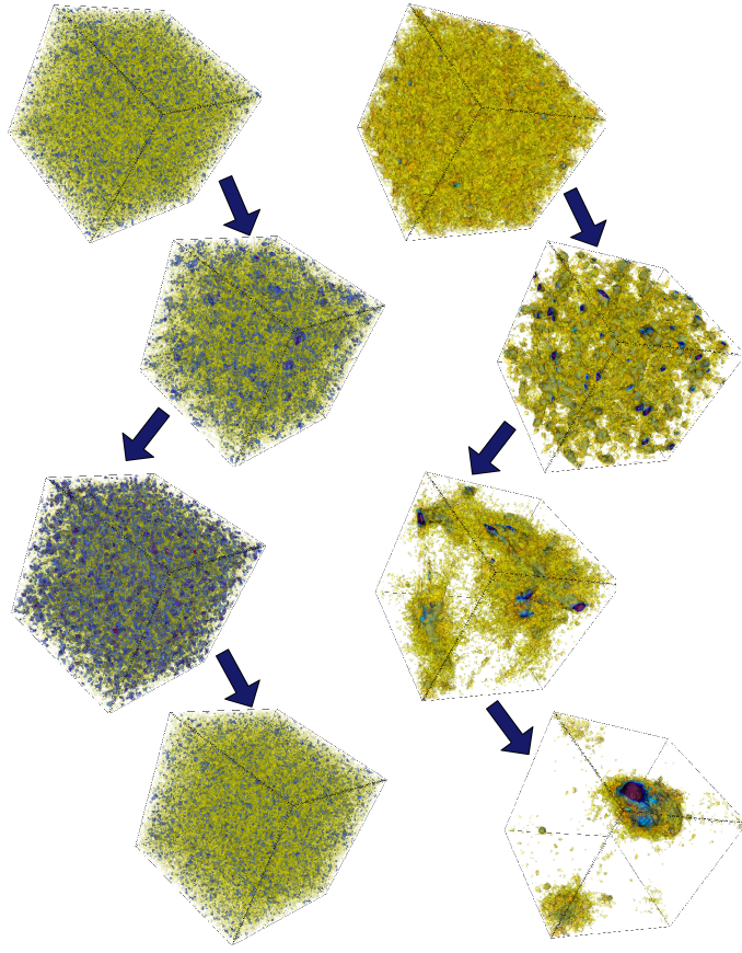
Figure 1: Snapshots of the number density contrast of neutrinos $\delta n_{\nu}(\vec{x})\equiv n_{\nu}(\vec{x})/\bar{n}_{\nu}-1$ at different times. Left: Model M2, at scale factors $a=0.45,\,0.7,\,0.75$ and $0.95$ from top to bottom. The overdensity oscillates between values close to 1 (represented as yellow tones) at early times, where there are no lumps, to values close to 10 (dark blue and purple tones), where several concentrated lumps form at intermediate times. At later times lumps dissolve and the overdensity decreases back to values close to unity. Right: Model M4, at scale factors: $a=0.35,\,0.42,\,0.53$ and $0.64$ from top to bottom. The neutrino lumps start growing at early times and merge progressively into larger and more concentrated structures. At the end, almost all neutrinos are attracted to a single very massive lump.

In contrast, the behavior for large neutrino masses is qualitatively different. The concentration of the lumps continues to grow after their first formation. Lumps merge, and typically do not dissolve. The neutrino number density contrast reaches high values at late times. This is demonstrated on the right panel in fig.1 for an average value of the neutrino mass $m_{\nu,av}=0.4$eV in the range $0.4<a<0.6$. This behavior resembles the one found for a constant cosmon-neutrino coupling in Ayaita et al. (2013, 2012); Baldi et al. (2011).

Due to the increasing value of the concentration and the increasing cosmon-neutrino coupling, the characteristic time scale becomes very short and gradients very large. This exceeds the present numerical capability of our simulations, typically at a value of the scale factor somewhat larger than $a=0.6$. In fig.2 we show snapshots for two different values of neutrino masses shortly before the simulation breaks down.

The transition between the “heating regime” for small neutrino masses and the “concentration regime” for large neutrino masses occurs in the range $\langle m_{\nu}\rangle[0.4:0.6]\approx 0.07\mbox{eV}-0.14\mbox{eV}$, where the time average is taken for $0.4<a<0.6$. The present value of the neutrino mass can be substantially larger due to oscillations and the continued increase of the mass and the temperature. For example, the phenomenologically viable model with $\langle m_{\nu}\rangle[0.4:0.6]=0.07$eV corresponds to a present neutrino mass of around $0.08$eV, but the time oscillations grow the neutrino mass to values of up to $0.5$eV for very short intervals in the scale factor $a$. (compare with fig. 5 below).

In fig.1 we show the distribution of the number (over)density contrast $\delta n_{\nu}(\vec{x})\equiv n_{\nu}(\vec{x})/\bar{n}_{\nu}-1$ at four different times and for two different models considered here, namely M2 (left panels) and M5 (right panels). For M2 as well as for models with smaller masses (not shown here), the neutrino lumps form and dissolve very quickly. The lumps are never stable and neutrinos accelerate to relativistic velocities when they fall into the gravitational potentials. The small lumps are also distributed homogeneously across the simulation box (see the third panel from above on the right of fig.1). The lumps reach maximal number density contrasts of about $\delta n_{\nu}\approx 10$. For M5 and for bigger masses, the neutrino lumps become stable, accreting more and more particles with the passing of time and increasing their concentrations. This leads to strong backreaction effects, changing the background cosmological evolution. After some time all neutrinos are concentrated in very big lumps, reaching very high values of $\delta{}_{\nu}\approx 50-100$, where $\delta_{\nu}\equiv\rho_{\nu}(\vec{x})/\bar{\rho}_{\nu}-1$, see fig.2. After this point, the numerical framework for the growing neutrino quintessence evolution breaks down and we can no longer solve reliably the coupled system of equations.

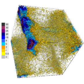
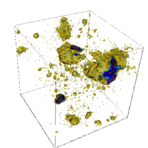
Figure 2: Snapshots of the neutrino overdensity field $\delta_{\nu}(\vec{x})$ for models M4 (top left) and M6 (bottom left) at scale factors of $a=0.64,\,$ and $0.62$, respectively. In these models, neutrino lumps cluster into large stable structures with a high concentration, starting from a bottom-up approach, as was shown for model M4 in fig. 1. Neutrino structures occupy large parts of the simulation box, corresponding to scales of ~50 Mpc. At these scale factors, the forces introduced by the cosmon coupling are too strong to be resolved by our numerical approach and our simulation breaks down.

V Cosmological evolution in the light neutrino regime

As we have seen in the previous section, there is a qualitative difference between the cosmological evolution of a model with a light or a heavy neutrino mass, the boundary being a present neutrino mass value of roughly $\approx 0.5$eV (calculated in linear theory). In this section we explore more in detail the evolution of background quantities in the light mass model M2 whose parameters are shown in detail in table 1 for the linear calculation in nuCAMB (top panel) and for the N-body computation (bottom panel). We study in detail the differences appearing in the evolution of background quantities, when non-linear physics and backreaction are taken into account.

The standard definition for the homogeneous energy density fraction of the cosmon field $\phi$ is

$$\Omega_{\phi}=\frac{8\pi G}{3H^{2}}\bar{\rho}_{\phi}\,\,,$$ (27)

where $\bar{\rho}_{\phi}$ is the background energy density of a homogeneous scalar field $\bar{\rho}_{\phi}=K(\phi)+V(\phi)$ and $K(\phi)$ its kinetic energy. In linear theory, the homogeneous term would be the only term entering into $\Omega_{\phi}$; on the contrary, within the N-body simulation, the field is non-homogeneous and the combined energy density of the coupled neutrino-cosmon fluid receives also a contribution from the perturbations $\delta\rho_{\phi}$ of the non-homogeneous cosmon field, given by eq.(18). The important quantity determining the evolution of a dynamical dark energy is not the energy density of the cosmon alone, but the energy density of the combined cosmon-neutrino fluid, given by

$$\Omega_{\phi+\nu}=\frac{8\pi G}{3H^{2}}\left(\bar{\rho}_{\phi}+\bar{\rho}_{\nu}\right)\,\,.$$ (28)

The average energy density of the neutrinos is not individually conserved and its evolution is given by the continuity equation with a coupling term on the r.h.s. Ayaita et al. (2012); Baldi et al. (2010)

$$\rho_{\nu}+2\mathcal{H}\rho_{\nu}=-\beta(\phi)\phi^{\prime}\rho_{\nu}\,\,,$$ (29)

where $\phi^{\prime}$ is the time derivative of the field with respect to conformal time $\tau$. The corresponding equation of state of the coupled fluid can then be defined as the sum of the pressure components divided by the sum of the density components

$$w_{\nu+\phi}=\frac{\bar{p}_{\phi}+\bar{p}_{\nu}}{\bar{\rho}_{\phi}+\bar{\rho}_{\nu}}\,\,.$$ (30)

In the literature Brookfield et al. (2007); Das et al. (2006); Perrotta et al. (1999); Perrotta and Baccigalupi (2002), there are several definitions of the effective equation of state or the observed equation of state in the case in which the scalar field is coupled to other particles. We argue that (30) is actually the equation of state one would observe from the evolution of the Hubble function (i.e. with Supernovae and standard candle methods of redshift distance measurements). In appendix B we comment further on this and show a comparison between the “observed” and theoretical equation of state of dark energy in fig.10.

In fig.3 we plot for model M2 the background evolution of the neutrino energy density $\Omega_{\nu}$ (orange lines) and the combined cosmon+neutrino fluid energy density $\Omega_{\nu+\phi}$ (blue lines) as defined in eq.(28). The dashed lines correspond to the linear computation in nuCAMB, while the solid lines correspond to the results of the N-body simulation. One can see that the effect of non-linearities and backreaction is quite small and it is mostly just visible as a phase shift in the oscillations of $\Omega_{\nu}$, which is due to the dynamics of the oscillating lumps, that alter the field-dependent mass of the neutrinos as a function of time and space. The same trend is observed in model M1 (not shown here). This behavior tells us that for small neutrino masses, the effects of backreaction on the background evolution are practically negligible and a linear computation is enough to analyze those models further, with a considerable simplification with respect to a joint linear and non-linear analysis done in Pettorino et al. (2010).

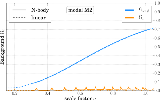
Figure 3: Evolution of $\Omega_{\phi+\nu}$ (blue lines) and $\Omega_{\nu}$ (orange lines) for Model M2, compared between the linear output from nuCAMB (dashed lines) and the non-linear calculation of the N-body simulation (solid lines). The total cosmon-neutrino fluid has the same background evolution in the simulation as in the linear calculation. The neutrino energy density is somewhat larger in the simulation and shows a phase-shift in its oscillations, as discussed in the text.

We show in fig.4 the neutrino equation of state $w_{\nu}$ (orange lines) as well as the combined cosmon-neutrino fluid equation of state $w_{\nu+\phi}$ as defined in equation 30 (blue lines), both for the case of the linear computation with nuCAMB (dashed lines) and the non-linear computation (solid lines). In the linear analysis, the neutrinos are treated initially as relativistic particles: as the mass increases, they become more and more non-relativistic, reaching a $w_{\nu}$ of exactly zero at late times. On the contrary, the N-body simulation is able to follow the oscillations in the equation of state of neutrinos, which are caused by the fact that neutrinos get accelerated to relativistic velocities when they fall into deep gravitational and cosmon potentials. Once they are in these lumps, and they have acquired high speeds, their pressure increases and they tend to escape again from these lumps, causing the oscillating neutrino structures. When they are far away from the cosmon potentials, their velocities decrease and they become non-relativistic again. The fifth force acting among neutrinos attracts them again to the cosmon potential wells and the whole cycle repeats itself.

For the combined equation of state $w_{\nu+\phi}$, we find that the simulation predicts a slightly higher value than the linear one; this can be explained by studying how the neutrino fluid is heated due to the strong oscillations of the lumps. By falling repeatedly in the cosmon potential wells and increasing their kinetic energy, the neutrinos temperature increases and therefore neutrinos do not manage to become again completely non-relativistic. This can be seen in the dashed orange lines of plot 4, where the curve of $w_{\nu}$ does not touch the zero axis after $a\approx 0.5$. We will see in section VI that neutrinos depart from their initial Fermi-Dirac distributions and reach temperatures which are high compared to the photon background.

Figure 4: Equation of state of the combined neutrino-cosmon fluid $w_{\phi+\nu}$ (blue) and equation of state of neutrinos $w_{\nu}$ (orange). We compare the linear output (dashed lines) to the non-linear one obtained from the N-body simulation (solid lines) for model M2. This model has a time averaged RMS mass $\langle m_{\nu}\rangle(a_{l})=0.164$, where $a_{l}=0.9$ in the label denotes the center of the time interval $a=[0.8-1.0]$ used to take the average. For $w_{\nu}$, the linear output does not capture the oscillating equation of state of neutrinos due to the formation of structures, while for $w_{\phi+\nu}$, both codes agree relatively well. At late times the equation of state predicted by the simulation has a somewhat higher value and is phase-shifted due to the heating of the neutrino fluid.

In fig.5, we show the evolution of the spatial average of the neutrino mass in the N-body simulation as a function of the scale factor $a$. One can see that the value of $\bar{m}_{v}$ varies along an order of magnitude, from approx.$10^{-2}$ to $10^{-1}$, throughout a cosmological time interval. Due to a phase shift in the oscillation pattern, which sets in at around $a\approx 0.8$, the present day value of the average neutrino mass can be quite different to the one estimated with the linear analysis (and this change depends on the precise parameters of the model), so that the best estimate for the average cosmological neutrino mass today, is a time average of $\bar{m}_{v}(\phi)$ at late times, between $a=0.8-1.0$. We can see that the big discrepancies between the masses of model M1 and M2 calculated in linear theory (e.g. Table 1 on page 1) are washed away when non-linearities and backreaction effects are taken into account i.e. for small neutrino masses. Even if the present neutrino masses for model M1 and M2 differ by an order of magnitude in linear theory, we find a very similar time averaged value between the two models in the N-body simulation: respectively $\langle m_{\nu}\rangle[0.8:1.0]=0.120$ and $\langle m_{\nu}\rangle[0.8:1.0]=0.164$. The oscillation pattern of the neutrino mass for the more massive model (M2) contains higher peaks and has a smaller frequency than compared to the oscillations in the less massive model M1. For other models, this comparison can be seen in table Table 1 on page 1.

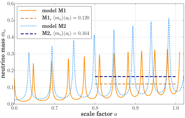
Figure 5: Neutrino mass $\overline{m}_{\nu}$ (average over simulation volume) in model M2 (firebrick red line) and model M1 (dodger blue line), as a function of the scale factor $a$, for the N-body simulation. The horizontal lines, show the time averaged RMS value at a late time $a_{l}=0.9$, denoting the center of the time interval of $[0.8:1.0]$ considered for taking the average. For model M2, the time averaged neutrino mass is $\langle m_{\nu}\rangle(a_{l})=0.164$ (blue dashed lines), while for model M1 it is somewhat smaller $\langle m_{\nu}\rangle(a_{l})=0.120$ (red dashed lines). One can observe that the oscillation frequency is higher for the smaller $\langle m_{\nu}\rangle$ mass and the peaks are higher for the larger $\langle m_{\nu}\rangle$. The present neutrino masses of the two models calculated in linear theory differ by an order of magnitude, on the contrary the time averaged masses are very close to each other.

VI heating of the neutrino fluid

The repeated acceleration of neutrinos to relativistic velocities during the periods of lump formation and dissolution lead to an effective heating of the neutrino fluid. While we do not expect a thermal equilibrium distribution of neutrino momenta and energies it is interesting to investigate how close the distribution is to the Fermi-Dirac distribution of a free gas of massive neutrinos. This distribution depends on only two parameters, the neutrino mass and the temperature. At a given time we associate the neutrino mass to the space averaged neutrino mass. The temperature can be associated to the mean value of the momentum.

The energy of a relativistic particle is given by

$$E(p,m)=\sqrt{p^{2}+m^{2}}\,\,,$$ (31)

while its kinetic energy $E_{k}=E(p,m)-m$. Equivalently, the kinetic energy is defined by

$$E_{k}=\int\vec{v}\>\cdot\mbox{d}\vec{p}\,\,,$$ (32)

which yields $E_{k}=m(\gamma-1)$ and reduces in the limit of very small velocities ($v\lll c$) to the usual $E_{k}=mv^{2}/2$. From there the Fermi-Dirac distribution as a function of momentum $p=|\vec{p}|$ can be obtained in the standard way. It depends on $m$ and $T$. For $m\ll T$ it can be approximated by the relativistic distribution while for $m\gg T$ we recover the Maxwell-Boltzmann distribution. The distribution of particle momenta is then given by

$$\mathcal{P}(p)\mbox{d}p=\frac{4\pi p^{2}}{(1+e^{(E(p,m)-\mu)/T})}\mbox{d}p$$ (33)

where the factor $4\pi$ comes form the angular integration of the three-dimensional momentum. In the ultra-relativistic limit we can analytically integrate the momentum $p$ over its distribution eq.(33) and invert $\bar{p}(\overline{T})$ to yield the mean temperature as a function of the mean momentum

$$\bar{T}=\frac{180\zeta(3)}{7\pi^{4}}\bar{p}$$ (34)

We neglect the chemical potential in (33), because the exponential term in the denominator is 2 or 3 orders of magnitude larger than unity. Since in our case, the average momentum and mass of the neutrinos are of the same order, we cannot use either a non-relativistic or an ultra-relativistic limit. We need to consider both the mass and the momentum in the relativistic energy equation (31). Therefore for each model and each time, we numerically find $\bar{T}$ as a function of the mean momentum $\overline{p}$.

We extract for $a=1$ the temperatures

$$\overline{T}=0.077\mbox{eV}\,\,\mbox{(M1, }\bar{m}_{\nu}=0.2404\mbox{)},\,\,\overline{T}=0.065\mbox{eV}\,\,\mbox{(M2, }\bar{m}_{\nu}=0.2327\mbox{)}\,\,.$$ (35)

They are higher by a factor 327 (M1) or 276 (M2) as compared to the CMB photon temperature $2.35\times 10^{-4}$eV. This demonstrates the unconventional heating of the neutrino fluid due to the formation and dissolution of lumps. The high temperatures are connected with the almost relativistic equation of state of the neutrinos seen in fig. 4. Overall, the observed momentum distributions come rather close to the thermal equilibrium distribution. This also holds for the distribution of kinetic energies. With the bulk quantities as momenta and kinetic energies roughly distributed thermally this is an example of prethermalization Berges et al. (2004).

In fig. (6) we fit the distribution of momenta of the neutrino particles on the grid (shown with an histogram) with a Fermi Dirac distribution. The actual distribution of momenta fits the thermal equilibrium distribution very well. At later times (orange shade), the fit is slightly less good: neutrinos might be accelerating towards or away from lumps giving them an extra kick that shifts the peak of the distribution of momenta.

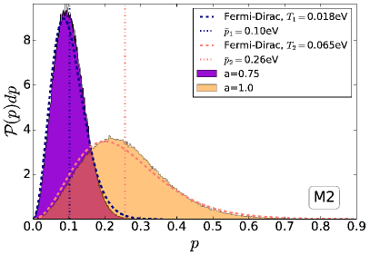
Figure 6: Distribution of the momenta of the neutrino particles in the simulation, for two different times, $a=0.75$ (purple shade) and $a=1.0$ (orange shade), compared against a Fermi-Dirac distribution with a temperature given by the mean of the distribution (dashed lines). Left: For model M1 the Fermi-Dirac fits very well for temperatures of $\bar{T}=0.018$eV and $\bar{T}=0.077$eV for each scale factor respectively. Right: For model M2 the fit is also good, the corresponding temperatures being $\bar{T}=0.018$eV and $\bar{T}=0.065$eV. The CMB photon temperature is $2.35\times 10^{-4}$eV, this means that the non-linear cosmon-neutrino interactions heat the neutrino background by more than a factor 100.

When comparing the equation of state of neutrinos obtained from the N-body simulation to a neutrino equation of state $w_{\nu}=p_{\nu}/\rho_{\nu}$, using our Fermi-Dirac fit to the particle distribution and eqns.(15) and (14), we get a very good agreement, taking into account that for the Fermi-Dirac fit, we are neglecting the spatial variation of the neutrino mass $m_{\nu}(\phi)$. For model M2 at the scale factor $a=0.75$ we obtain from the N-body simulation a neutrino equation of state of $w_{\nu}=0.081$ while using the Fermi-Dirac fit to the distribution of particles with a mean temperature of $\bar{T}=0.018$eV and an average neutrino mass $\bar{m}_{\nu}=0.1835$, the proper calculation yields $w_{\nu}=0.086$. For a later time, at $a=1.0$ the N-body simulation gives us a value of $w_{\nu}=0.207$ while the Fermi-Dirac fit with a mean temperature of $\bar{T}=0.065$eV and an average neutrino mass $\bar{m}_{\nu}=0.2327$ amounts to a neutrino equation of state of $w_{\nu}=0.182$.

To visualize the evolution of $w_{\nu}$, we can observe from fig.4 that neutrinos in the N-body simulation start as non-relativistic particles and oscillate between being almost relativistic and completely non-relativistic in the interval $a=[0.3,0.6]$. However, at later times $a\apprge 0.7$ the neutrino equation of state still oscillates but never reaches a value of zero again. This is in agreement with our description of the heating of the neutrino fluid. Since the mean temperature of the neutrino fluid is increasing with time and therefore its mean kinetic energy and pressure, the minimum of the oscillations of the neutrino equation of state increases also in time and departs from zero, once neutrinos are heated to very high temperatures due to the collapsing and dissolving of the neutrino-cosmon lumps.

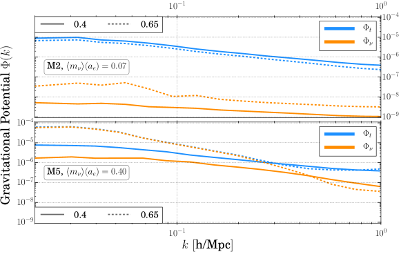
Figure 7: Power spectra of the total gravitational potential $\Phi_{t}$ (blue lines) and of the neutrino contribution $\Phi_{\nu}$ (orange lines) for model M2 and model M5 at the scale factors $a=0.40$ (solid lines) and $a=0.65$ (dashed lines), as a function of scale. Model M2 has an RMS time averaged neutrino mass $\langle m_{\nu}\rangle(a_{e})=0.07$, where $a_{e}=0.5$ stands for the central time in the interval $a=[0.4-0.6]$ used to take the average. Model M5 has in the same interval a higher RMS mass of $\langle m_{\nu}\rangle(a_{e})=0.40$. In the first model, $\Phi_{t}$ at large scales is of the order of $10^{-5}$, while $\Phi_{\nu}$ is 3 to 4 orders of magnitude smaller at both cosmological times. For model M5, in which neutrino lumps are stable and growing, one sees that at large scales, the total $\Phi_{t}$ starts with a value of $10^{-5}$ at $a=0.4$, but reaches $10^{-4}$ at later times. At $a=0.65$ the neutrino contribution is dominant and neutrino structures have migrated from small scales to large scales, as can be seen from the dip in $\Phi_{\nu}$ at modes between $k=0.2-1.0$ h/Mpc.

VII Gravitational Potentials of Neutrino Lumps

The gravitational potential $\Phi$ is a good measure of the physics going on in structure formation. We know from observational constraints, that $\Phi$ is of the order of $10^{-5}$ on cosmological scales Pettorino et al. (2010); Brouzakis et al. (2011). In $\Lambda\textrm{CDM}$, the gravitational potential is sourced mainly by dark matter perturbations. In figures 7 and 8 we show that for models with small neutrino masses, the neutrino contribution to $\Phi$ remains several orders of magnitude smaller than the CDM contribution, at all scales and at all times. Moreover, one can observe an oscillation in time of the neutrino gravitational potential. For models with large neutrino masses, the neutrino contribution grows monotonically with time. At large scales $k\lesssim 0.3$h/Mpc and at late times the neutrino lump induced potential dominates over the cold dark matter gravitational potential. This renders the total potential $\Phi_{tot}$ too big to be compatible with present cosmological constraints.

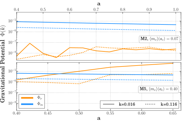
Figure 8: Power spectra of the matter gravitational potential $\Phi_{m}$ (blue lines) and of the neutrino contribution $\Phi_{\nu}$ (orange lines) at two different scales, $k=0.016$ (solid lines) and $k=0.116$ (dashed lines) as a function of scale factor $a$ with two different scales on the top and bottom axis. For model M2 the matter gravitational potential $\Phi_{m}$ is at most $10^{-5}$ at all times, while the neutrino contribution is 2-3 orders of magnitude smaller and displays time oscillations. In clear contrast, the neutrino contribution from model M5 for very large scales, reaches and dominates over the matter contribution for $a\apprge 0.5$ and pushes the total $\Phi$ to high values that would be ruled out by observations, see also fig. 7. The RMS neutrino mass has been taken in the same interval range as for fig.7, where $a_{e}=0.5$.

We show the scale dependence of the total gravitational potential and the neutrino induced gravitational potential $\Phi_{\nu}$ at two different cosmic time scales $a=0.4$ and $a=0.65$ in fig.7. While for $a=0.4$ (solid lines) the neutrino contribution is still subdominant for both models M2 and M5, this changes at $a=0.65$ for model M5 (bottom panel). For model M2 the total gravitational potential decreases in time, as it is expected due to the effect of dark energy, while $\Phi_{\nu}$ increases especially at large scales. For model M5, since the neutrino contribution dominates at $a=0.65$, the total gravitational potential is raised to values of $10^{-4}$ at large scales, while at small scales ($k\apprge 0.4$) the neutrino contribution is still subdominant.

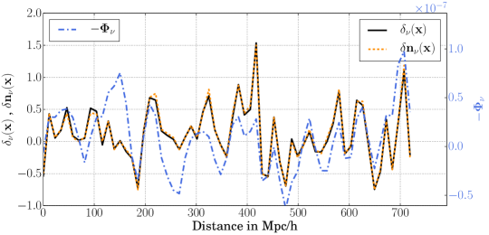
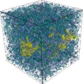
Figure 9: Left: Line plot through the main diagonal of the simulation box, for model M2 at $a=0.75$. The negative of the neutrino contribution to the gravitational potential $\Phi_{\nu}$ (blue dot-dashed lines) oscillates between $\pm 1.0\times 10^{-7}$. This is correlated to the neutrino density contrast (black lines) and the number density contrast $\delta n_{\nu}=n_{\nu}(\vec{x})/\bar{n}_{\nu}-1$ (orange dashed lines) reaching values of up to 1.5. Right: Snapshot of the same simulation, showing a equipotential contour of the gravitational potential, for $\Phi_{\nu}=+1.0\times 10^{-7}$ in yellow, and the small but dense neutrino lumps in blue, purple and red, corresponding to density contrasts $\delta n_{\nu}$ of 1.5, 2.0 and 4.0 respectively.

In fig.8 we show the power spectra of the total gravitational potential $\Phi$ (blue lines) and of the neutrino contribution to it (orange lines) at two different scales, $k=0.016$ (solid lines) and $k=0.116$ (dashed lines) as a function of the scale factor $a$. For model M2, corresponding to an average early time neutrino mass of 0.07 eV, the total gravitational potential $\Phi(k)$ is $10^{-5}$ at all times, while the neutrino contribution is 2-3 orders of magnitude smaller and shows time oscillations. In clear contrast, the neutrino contribution from model M5 (corresponding to an average early time neutrino mass of 0.40 eV)) for very large scales reaches and dominates over the matter contribution (at $a\apprge 0.5$) and pushes the total $\Phi$ to high values that would be ruled out by observations. This is due to the fact that neutrino lumps do not dissolve, but rather grow with continuously growing concentration and higher gravitational potential.

There is also anticorrelation between the neutrino structures and the neutrino induced gravitational potential, as expected from the fact that neutrinos will tend to fall into gravitational potential wells. In the left panel of fig.9, we plot the values of the neutrino number density contrast $\delta n_{\nu}=n_{\nu}(\vec{x})/\bar{n}_{\nu}-1$ and the negative neutrino induced gravitational potential $\Phi_{\nu}$, along a diagonal line through the simulation box. The correlation of peaks and troughs (corresponding to an anticorrelation of $\delta n_{\nu}$ and $\Phi_{\nu}$) is very clear and it is valid for even small substructures of the order of a few Mpc. By plotting the neutrino density contrast $\delta_{\nu}$, we also show that at this time $a=0.75$, the neutrino number density and the energy density are proportional, meaning that neither local mass variations or relativistic speeds are having any effect in the neutrino total energy. In the right panel of fig.9 we visualize the neutrino induced gravitational potential as a yellow region marking the equipotential surface $\Phi_{\nu}=+1.0\times 10^{-7}$ and the neutrino number overdensity structures colored blue, purple and red, corresponding to density contrasts $\delta n_{\nu}$ of 1.5, 2.0 and 4.0 respectively. For this model (M2) and at this specific time, the neutrino structures are spread almost homogeneously throughout the simulated volume.

VIII Conclusions

We have investigated the dynamics of neutrino lumps in growing neutrino quintessence and how it depends on the mass of neutrinos. As a main result of this paper we found a characteristic divide in the qualitative behavior between small and large neutrino mass.

For light neutrino masses the combined effects of oscillations in the neutrino masses and the cosmon-neutrino coupling lead to rapid formation and dissociation of the neutrino lumps. The concentration in the neutrino structures never grows to very large overdensities. As a consequence, backreaction effects remain small. The effects of lump formation and dissociation lead to an effective heating of the neutrino fluid to temperatures much higher than the photon temperature. Due to this heating, the neutrino equation of state becomes again close to the one for relativistic particles. For a small present average neutrino mass $m_{\nu}=0.06$eV it has been found earlier Pettorino et al. (2010) that the cosmology of growing neutrino quintessence resembles very closely a cosmological constant, making differences to the $\Lambda\textrm{CDM}$ model difficult to detect. We extend this qualitative feature to a whole range of light neutrino masses.

For large neutrino masses, one finds a qualitatively different behavior. Big neutrino lumps form, due to the strong cosmon-mediated fifth-force between neutrinos. These lumps are stable and keep growing in concentration and density. The strong clumping of the cosmic neutrino background induces large backreaction effects on the overall cosmic evolution. As a result, the combined cosmon-neutrino fluid does not act effectively as a cosmological constant anymore and compatibility with observations is difficult to achieve. This situation is similar to the case of a constant cosmon-neutrino coupling Führer and Wetterich (2015).

The divide in the characteristic behavior reflects the competition between heating of the neutrino fluid and lump concentration. We have not yet established a quantitatively accurate value of the parameter $\hat{m}_{\nu}$ where the divide is located, since the numerics are rather time consuming. In principle, this divide will lead to an upper bound on the present neutrino mass, as seen in terrestrial experiments. For models in the vicinity of model M2, which seem compatible with observations so far, spatial average neutrino masses as large as $0.5$eV can occur at the peak of oscillations, c.f. fig.5. We note that if we live inside a neutrino lump the neutrino mass will be reduced as compared to the cosmological value.

We have further computed the strength of the neutrino-induced gravitational potential. For light masses, this potential is found to be rather small, rendering a detection of the neutrino lumps difficult. As neutrino masses increase towards an intermediate mass region, before reaching the heavy mass range incompatible with observation, the neutrino-induced gravitational potentials will get stronger. By continuity we expect that in the intermediate mass region the clumped neutrino background becomes observable.

Appendix A Initial parameters for generating the models in nuCAMB and in the N-Body simulation

CAMB values	M1	M2	M3	M4	M5	M6
input: $\Omega_{\nu}h^{2}$	0.048	0.048	0.075	0.018	0.038	0.098
$\tilde{m}_{\nu}$ amplitude factor	$8.35\times 10^{-5}$	$2.0\times 10^{-4}$	$6.0\times 10^{-4}$	$9.9\times 10^{-3}$	$8.8\times 10^{-3}$	$8.8\times 10^{-3}$
input $\hat{r}_{\nu eV}$ factor	1.5045	1.5045	2.3508	0.5642	1.1911	3.0718
$V_{i}$	$0.99\times 10^{-7}$	$0.99\times 10^{-7}$	$0.99\times 10^{-7}$	$0.99\times 10^{-7}$	$0.99\times 10^{-7}$	$0.99\times 10^{-7}$

Table 2: Table of initial parameters for each model computed with nuCAMB. $\tilde{m}_{\nu}$ is the neutrino mass amplitude used in the simulations, $\hat{r}_{\nu eV}$ is the neutrino mass units conversion factor between the simulations and nuCAMB. $V_{i}$ is the initial value of the cosmon potential.

N-body parameters	Values	Meaning
$L$	$428$	Box side length in Mpc/h
$N_{g}$	64	Grid size per dimension
$N_{pdm}$	262144	Number of dark matter particles in the simulation
$N_{p\nu}$	524288	Number of neutrino particles in the simulation
$\mbox{ngs}_{\mbox{acc}}$	$1.0\times 10^{-5}$	Numerical accuracy for the NGS solver

Table 3: Table of numerical parameters for each N-body simulation run. Several tests were performed varying these parameters, but the overall behavior for the purposes of this paper was the same. We also tested model M2 with grid sizes of 128 and 8 times the number of particles, not noticing any qualitative difference in the dynamics. Only deviations of the order of 10% in perturbation quantities were observed when varying the grid size or the number of particles.

Appendix B The effective and observed equation of state of dark energy

The equation of state $w$ of a species is defined in terms of its pressure and density as

$$w=\frac{p}{\rho}\,\,\,.$$ (36)

For the case of coupled species, there have been several definitions in the literature (c.f. Brookfield et al. [2007], Das et al. [2006], Perrotta et al. [1999], Perrotta and Baccigalupi [2002]). This is due to the fact that when there is an exchange of energy and momentum between a particle and a scalar field, the time evolution of matter does not correspond anymore to the volume dilution rule $\rho(a)=\rho_{0}a^{-3}$. Therefore the equation of state of the dark energy field will not be as simple as the equation of state of a homogeneous scalar field, namely

$$w_{\phi}=\frac{p_{\phi}}{\rho_{\phi}}=\frac{(1/2a^{2})\dot{\phi}^{2}+V(\phi)}{(1/2a^{2})\dot{\phi}^{2}-V(\phi)}\,\,\,.$$ (37)

In Das et al. [2006], Brookfield et al. [2007] two definitions of the equation of state (e.o.s) of dark energy were investigated. The first one, called the effective e.o.s. $w_{eff}$, given by

$$w_{eff}\equiv w_{\phi}+\frac{\beta\dot{\phi}}{3H}\frac{\rho_{\nu}}{\rho_{\phi}}$$ (38)

and the second one named “apparent” e.o.s. $w_{ap}$, defined by

$$w_{ap}\equiv\frac{w_{\phi}}{1+x}\,\,\,,$$ (39)

with

$$x=-\frac{\rho_{\nu,0}}{a^{3}\rho_{\phi}}\left[\frac{m_{\nu}(\phi)}{m_{\nu}(\phi_{0})}-1\right]\,\,\,,$$ (40)

where a $0$ subscript denotes quantities at $z=0$. Notice that by construction, $w_{ap}$ at the present epoch is identical to $w_{\phi}$ and that $w_{ap}$ can be smaller than $-1$. We find that none of these two definitions of e.o.s. describe the dynamical dark energy field present in our model.

Since in our model the neutrino and cosmon field behave together as a tightly coupled fluid, we are interested in the conserved equation of state for the combined fluid. This is given by the sum of both contributions from the pressure, divided by the sum of both densities. Therefore, we define $w_{\nu+\phi}$ as

$$w_{\nu+\phi}\equiv\frac{\bar{p}_{\phi}+\bar{p}_{\nu}}{\bar{\rho}_{\phi}+\bar{\rho}_{\nu}}\,\,\,.$$ (41)

This definition should agree with what we can extract directly from observations of the Friedmann equation. The equation of state $w_{DE}(z)$ of a general dark energy component that fulfills the continuity equation (if it is composed by two coupled fluids, the continuity equation is fulfilled for the sum of densities and pressures), appears in the Friedmann equation as

$$E^{2}(z)\equiv\frac{H^{2}(z)}{H_{0}^{2}}=\left[\Omega_{r,0}(1+z)^{4}+\Omega_{m,0}(1+z)^{3}+\Omega_{DE,0}\exp\left\{\int_{0}^{z}\frac{3(1+w_{DE}(\tilde{z}))}{1+\tilde{z}}\mbox{d}\tilde{z}\right\}+\Omega_{k,0}(1+z)^{2}\right]\,\,\,.$$ (42)

Moreover, in a flat Universe and with a negligible contribution from radiation, we can solve for $w_{DE}(z)$ and obtain Amendola and Tsujikawa [2010]:

$$w_{DE}(z)=\frac{(1+z)(E^{2}(z))^{\prime}-3E^{2}(z)}{3\left[E^{2}(z)-\Omega_{m,0}(1+z)^{3}\right]}\,\,\,.$$ (43)

Thus, from background expansion observations we can obtain a constrain on $w_{DE}(z)$, provided we know from large-scale structure or CMB observations the present value of $\Omega_{m}$. In the fig. 10 we compare $w_{DE}(z)$ obtained from eq.(43) and $w_{\nu\phi}(z)$ computed both consistently within the N-body simulation. In the former case, numerical noise in the derivatives of $E(z)$ create certain scatter in $w_{DE}(z)$ at late times.

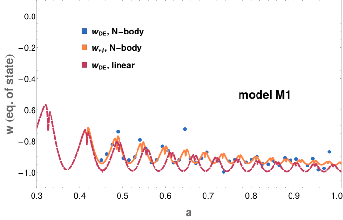
Figure 10: Different $w(z)$ curves in the case of model M1 computed with the N-body simulation and compared to linear theory. The red dashed lines represent $w_{DE}$ computed from the Hubble function which is an output of the linear code nuCAMB. The solid orange line, representing $w_{\nu+\phi}$ is computed using the standard pressure and density outputs from the simulation. The blue dots stand for some set of computed values of $w_{DE}(z)$ obtained from the Hubble function calculated entirely within the N-body simulation. Due to numerical noise in the oscillating derivatives of $E(z)$, there is some scatter in the e.o.s. obtained in this case.