Mapping the Real Space Distributions of Galaxies in SDSS DR7: I. Two Point Correlation Functions

Abstract

Using a method to correct redshift space distortion (RSD) for individual galaxies, we mapped the real space distributions of galaxies in the Sloan Digital Sky Survey (SDSS) Data Release 7 (DR7). We use an ensemble of mock catalogs to demonstrate the reliability of our method. Here as the first paper in a series, we mainly focus on the two point correlation function (2PCF) of galaxies. Overall the 2PCF measured in the reconstructed real space for galaxies brighter than $\>{}^{0.1}{\rm M}_{r}-5\log h=-19.0$ agrees with the direct measurement to an accuracy better than the measurement error due to cosmic variance, if the reconstruction uses the correct cosmology. Applying the method to the SDSS DR7, we construct a real space version of the main galaxy catalog, which contains 396,068 galaxies in the North Galactic Cap with redshifts in the range $0.01\leq z\leq 0.12$. The Sloan Great Wall, the largest known structure in the nearby Universe, is not as dominant an over-dense structure as appears to be in redshift space. We measure the 2PCFs in reconstructed real space for galaxies of different luminosities and colors. All of them show clear deviations from single power-law forms, and reveal clear transitions from 1-halo to 2-halo terms. A comparison with the corresponding 2PCFs in redshift space nicely demonstrates how RSDs boost the clustering power on large scales (by about $40-50\%$ at scales $\sim 10\>h^{-1}{\rm{Mpc}}$) and suppress it on small scales (by about $70-80\%$ at a scale of $0.3\>h^{-1}{\rm{Mpc}}$).

1. Introduction

One of the important properties of the galaxy population is the distribution of galaxies in space (e..g. Peebles, 1980; Mo et al., 2010). This distribution can be used to infer the large scale mass distribution in the universe, thereby constraining cosmological models (e.g. Fisher et al., 1994; Peacock et al., 2001; Hawkins et al., 2003; Yang et al., 2004; Tinker et al., 2005). Furthermore, the spatial clustering of galaxies is also one of the key pieces of observational data to establish the relation between galaxies and dark matter (halos) statistically (e.g. Jing et al., 1998; Peacock & Smith, 2000; Yang et al., 2003, 2012), and to understand how galaxies form and evolve in the cosmic density field.

One of the main goals of large redshift surveys of galaxies, such as the 2 degree Field Galaxy Redshift Survey (2dFGRS; Colless et al., 2001) and the Sloan Digital Sky Survey (SDSS; York et al., 2000) is, therefore, to provide a data base to study the three dimensional distribution of galaxies as accurately possible. However, a key problem this endeavor is that redshifts of galaxies are not exact measures of distances due to the peculiar motions of galaxies. The spatial distribution and clustering of galaxies observed in redshift space are thus distorted with respect to the real-space distribution and clustering (e.g. Sargent & Turner, 1977; Davis & Peebles, 1983; Kaiser, 1987; Regos & Geller, 1991; Hamilton, 1992; van de Weygaert & van Kampen, 1993). Take the two-point correlation function (2PCF) of galaxies as an example. The 2PCF in the 2-dimensional space, with 1 dimension along the line-of-sight and the other in the perpendicular direction, appears elongated on small scales and squashed on large scales along the line-of-sight direction, in contrast to an isotropic pattern expected from a statistically homogeneous and isotropic distribution in real space. Such anisotropies are clearly produced by redshift distortions and need to be corrected in order to get the true distribution of galaxies in space. Theoretically, models of the pairwise peculiar velocities of galaxies have been used to model the effects of redshift distortions on the measured 2PCF in redshift space (e.g. Davis & Peebles, 1983; Fisher et al., 1994; Jing et al., 1998). Alternatively, one simply measures the projected 2PCF and uses it to infer the three-dimensional 2PCF (e.g. Jing et al., 1998; Li et al., 2006; Zehavi et al., 2011).

In the gravitational instability scenario of structure formation, the redshift distortion is not just a contamination one has to correct in order to get the real clustering of galaxies, it in fact contains useful information about cosmology as well as the mass distribution in the universe. On large scales, the infall motions of galaxies, which produce the squashing in the 2D redshift-space 2PCF (the Kaiser effect, Kaiser, 1987), is linearly proportional to the amplitudes of the mass density fluctuations on large-scales. In this case, one can compute the quadrupole-to-monopole ratio of the 2D 2PCF to get $\beta\equiv f(\Omega_{\rm m})/b$, where $\Omega_{\rm m}$ is the density parameter of mass, and $b$ is the effective linear bias of the galaxies in question (e.g. Guzzo et al., 2008; Samushia et al., 2012; Dawson et al., 2016, and references therein). When the measurement is combined with weak gravitational lensing results, it can also be used as a sensitive probe of (modified) gravitation theories on cosmology scales (Zhang et al., 2007; Reyes et al., 2010; Blake et al., 2016). On smaller scales, the modeling of redshift space distortion (the Finger of God effect, Jackson, 1972; Tully & Fisher, 1978) is complicated by the nonlinear mapping between real-space and redshift-space. Great efforts have been made not only to understand its impacts on galaxy clustering (e.g. Zhang et al., 2013; Zheng et al., 2013; Zhang et al., 2015; Zheng et al., 2015a, b), but also to extract useful cosmological information (Mo, Jing & Boerner 1993; Jing, Mo & Boerner 1998; Yang et al. 2004; Li et al. 2012).

The approaches adopted earlier to deal with redshift distortions in galaxy clustering have been hampered by the fact that the large-scale Kaiser effect and the small-scale Finger of God effect are interwoven, and models based on a simple pairwise peculiar velocity distribution can only be served as an approximation. The situation is complicated even more by the fact that the effect bias in galaxy distribution may be nonlinear and its form is not known a priori. Models based on the projected correlation function has its own problem, because the projection mixes clustering on different scales so that the conversion from the projected function to the three dimensional function can be uncertain. Thus, in order to make full use of galaxy redshift surveys to study the large-scale structure of the universe, a change of tactics is needed.

One possible way is first to make corrections of redshift distortions for individual galaxies, and then use the ‘pseudo’ real space distribution of galaxies to derive statistical measures of galaxy clustering in real space. As mentioned above, redshift distortions are of two different kinds. One is the Kaiser effect produced by the coherent flow due to the gravitational action of large-scale structure (Kaiser, 1987), the other is the Finger of God (FOG) effect generated by the random motions of galaxies within virialized halos on small scales. To deal with the FOG effect, Tegmark et al. (2002) used an friends-of-friends method to link galaxies and suppressed the over-density of the pairs along the line of sight by a factor of 10. They applied this FOG suppression to the 2dFGRS (Tegmark et al., 2002) and SDSS (Tegmark et al., 2004) in their estimates of the power spectra of galaxy distribution. In a paper aimed at reconstructing the cosmic web from 2dFGRS, Erdoǧdu et al. (2004) attempted to dealt with the FOG effect by compressing 25 fingers seen in redshift space using groups identified by Eke et al. (2004). For the Kaiser effect, Yahil et al. (1991) used a bias model to get the density field from the galaxy distribution and iteratively corrected the infall motions of galaxies. Along the same line, a number of approaches have been taken to recover/correct the infall motions on the basis of galaxy distribution (e.g. Monaco & Efstathiou, 1999; Lavaux et al., 2008; Wang et al., 2009; Branchini et al., 2012; Wang et al., 2012; Kitaura et al., 2012; Granett et al., 2015; Jasche et al., 2015; Kitaura et al., 2016; Ata et al., 2016). In particular, Wang et al. (2009, 2012) used galaxy groups as proxies of dark matter halos to reconstruct the density field, which in turn was used to obtain the velocity field.

So far there has been no real attempt to correct for both the large scale velocities and small scale random motions of galaxies in a systematic way. The main purpose of the present paper is to carry out such an investigation, using galaxies observed in the SDSS DR7, which is still among the best redshift surveys available. Based on this galaxy catalog, Yang et al. (2007, hereafter Y07) have constructed a galaxy group catalog using an adaptive halo-based group finder (see also Yang et al., 2005). Detailed tests with mock galaxy catalogues have shown that the group finder is very successful in associating galaxies according to their common dark matter halos. In particular, the group finder performs reliably not only for rich systems, but also for poor systems, including isolated central galaxies in low mass halos. The reliable memberships of galaxies in groups provide a unique opportunity to correct for the FOG effects for individual galaxy systems. In addition, as shown in Wang et al. (2012, hereafter W12), the group catalog can also be used to reconstruct the mass density, tidal and velocity (MTV) fields in the SDSS DR7 volume, using the halo-domain method developed in Wang et al. (2009). Since the relation between halo and mass distributions is better understood than that between galaxies and mass, the mass and velocity fields constructed are much more accurate than those constructed directly from the galaxy distribution. The redshift distortions on large scales can, therefore, also be modeled accurately for individual galaxies. With all these, we can obtain a catalog of galaxies in quasi-real space. We can then not only examine in detail various types of redshift distortions, but also measure the real space clustering of galaxies.

This paper is organized as follow. In Section 2 we present the galaxy and group catalogs used in this paper. Section 3 introduces the methods to correct for the redshift distortions and to characterize the galaxy clustering. In Section 4 we use mock galaxy catalogs to test the reliability of our correction model. The application to the SDSS DR7 and the results are presented in Section 5. Finally, we summarize our main findings in Section 6. Throughout this paper, unless stated otherwise, physical quantities are quoted using the WMAP9 cosmological parameters (Hinshaw et al., 2013): $\Omega_{\rm m}=0.282$, $\Omega_{\Lambda}=0.718$, $\Omega_{\rm b}=0.046$, $n_{\rm s}=0.965$, $h=H_{0}/(100\>{\rm km}\,{\rm s}^{-1}\,{\rm Mpc}^{-1})=0.697$ and $\sigma_{8}=0.817$.

[c] Absolute Magnitude Flux-limited Volume-limited $\>{}^{0.1}{\rm M}_{r}-5\log h$ Redshift    $N_{gal}$($N_{blue}$/$N_{red}$) Averaged Magnitude Redshift    $N_{gal}$($N_{blue}$/$N_{red}$) Averaged Magnitude $\bm{[}-23,-22\bm{]}$ $\bm{[}0.01,0.12\bm{]}$ $~{}~{}~{}2200(379/1821)$ $-22.22$ $\bm{[}0.01,0.12\bm{]}$ $~{}~{}~{}2200(379/1821)$ $-22.22$ $\bm{[}-22,-21\bm{]}$ $\bm{[}0.01,0.12\bm{]}$ $~{}~{}~{}42207(11997/30210)$ $-21.34$ $\bm{[}0.01,0.12\bm{]}$ $~{}~{}~{}42207(11997/30210)$ $-21.34$ $\bm{[}-21,-20\bm{]}$ $\bm{[}0.01,0.12\bm{]}$ $~{}~{}~{}156765(64956/91809)$ $-20.44$ $\bm{[}0.01,0.113\bm{]}$ $~{}~{}~{}134801(55572/79229)$ $-20.43$ $\bm{[}-20,-19\bm{]}$ $\bm{[}0.01,0.12\bm{]}$ $~{}~{}~{}127444(71018/56426)$ $-19.57$ $\bm{[}0.01,0.075\bm{]}$ $~{}~{}~{}73391(41659/31732)$ $-19.47$ $\bm{[}-19,-18\bm{]}$ $\bm{[}0.01,0.12\bm{]}$ $~{}~{}~{}43894(31646/12248)$ $-18.58$ $\bm{[}0.01,0.045\bm{]}$ $~{}~{}~{}21875(16052/5823)$ $-18.48$ $\bm{[}-18,-17\bm{]}$ $\bm{[}0.01,0.12\bm{]}$ $~{}~{}~{}17259(14327/2932)$ $-17.57$ $\bm{[}0.01,0.026\bm{]}$ $~{}~{}~{}5618(4818/800)$ $-17.46$

Table 1Galaxy Subsamples

2. The SDSS galaxy and group catalogs

The galaxy sample used in this paper is constructed from the New York University Value-Added Galaxy Catalog (NYU-VAGC; Blanton et al., 2005), which is based on SDSS DR7 (Abazajian et al., 2009), but with an independent set of significantly improved reductions over the original pipeline. In addition, as galaxy groups play a key role in our approach to correct for the redshift distortions, we make use of the group catalog constructed in (Yang et al., 2012, hereafter Y12) for SDSS DR7. This group catalog is based on all galaxies in the Main Galaxy Sample with extinction-corrected apparent magnitude brighter than $r=17.72$, with redshifts in the range $0.01\leq z\leq 0.20$ and with a redshift completeness $C_{z}>0.7$. The catalog contains a total of 639,359 galaxies with a sky coverage of 7,748 deg². Moreover, the galaxy catalog mainly covers two sky regions: a larger contiguous region in the Northern Galactic Cap (NGC) and a smaller three-stripe region in the Southern Galactic Cap (SGC). The former contains 584,473 galaxies with a sky coverage of 7,047 deg².

Based on this SDSS DR7 galaxy catalog, Y12 used the adaptive halo-based group finder developed by Y05 to select galaxy groups. This group finder has been applied to the SDSS DR4 in Y07. Following Y07, the masses of the associated dark matter halos are estimated based on the ranking of the total characteristic luminosities of groups or the total characteristic stellar masses using group member galaxies more luminous than $\>{}^{0.1}{\rm M}_{r}-5\log h=-19.5$. Both halo masses agree very well with each other, and we adopt the halo masses based on the characteristic luminosity ranking in this paper. In addition, we have updated group membership as well as halo masses according to WMAP9 cosmology.

Using this group catalog, W12 reconstructed the velocity field, which we use in this paper to correct for the redshift space distortions. The method of W12 explicitly depends on the density field as represented by dark matter halos above a given mass threshold, $M_{\rm th}$. We adopt $M_{\rm th}=10^{12.5}h^{-1}M_{\sun}$ and so, to be complete, restrict our sample to the nearby volume covering the redshift range $0.01\leq z\leq 0.12$. In addition, since the W12 reconstruction method can be significantly impacted by survey boundaries, we focus only on the more contiguous NGC region.

Applying all these selection criteria to the galaxy and group catalogs leaves us with a set of 286,043 groups, hosting a total of 396,068 galaxies in the NGC region with redshifts in the range $0.01\leq z\leq 0.12$. Finally, using this sample we construct both flux-limited and volume-limited subsamples for galaxies in the following six absolute $r$-band magnitude bins: $\>{}^{0.1}{\rm M}_{r}-5\log h=$ $\bm{[}-23.0,-22.0\bm{]}$, $\bm{[}-22.0,-21.0\bm{]}$, $\bm{[}-21.0,-20.0\bm{]}$, $\bm{[}-20.0,-19.0\bm{]}$, $\bm{[}-19.0,-18.0\bm{]}$ and $\bm{[}-18.0,-17.0\bm{]}$. The corresponding redshift ranges, numbers of galaxies and averaged magnitude are indicated in Table 1. These luminosity samples are further divided into blue and red subsamples, as detailed in Section 5.2. Note that there is no difference in the redshift limit between the flux-limited and volume-limited for the first two brightest samples, because all the galaxies with such luminosities can be observed to $z=0.12$. For a fainter sample, even the brightest galaxies in the luminosity bin can be observed only to redshift $z<0.12$. In most cases we only show results obtained from the flux limited samples, because the results obtained from the volume limited samples are very similar. Note also that in the reconstructed real space, which we will perform later, the number of galaxies in a sample will change very slightly.

SPACE	DESCRIPTION
Real space	survey geometry without redshift distortions
FOG space	distorted only by FOG effect:   $z_{\rm obs}=z_{\rm cos}+\frac{v_{\sigma}}{c}(1+z_{\rm cos})$
Kaiser space	distorted only by Kaiser effect:   $z_{\rm obs}=z_{\rm cos}+\frac{v_{\rm cen}}{c}(1+z_{\rm cos})$
Redshift space	distorted by both Kaiser and FOG effects:   $z_{\rm obs}=z_{\rm cos}+\frac{v_{\rm pec}}{c}(1+z_{\rm cos})$
Re-real space	reconstructed real space; based on correcting redshift space distortions
Re-Kaiser space	reconstructed Kaiser space; based on correcting for FOG effect only
Re-FOG space	reconstructed FOG space; based on correcting for Kaiser effect only

Notes. The first four spaces are ‘true’ spaced, based on true groups (all galaxies belonging to the same dark matter halo). The final three space are ‘reconstructed’ spaces based on groups identified applying the group finder in redshift space.

Table 2Description of different spaces.

3. METHODOLOGY AND BASIC ANALYSIS

We now turn to our main goal: correcting the SDSS redshifts for redshift space distortions induced by peculiar velocities, thus allowing for a direct measurement of the two-point correlation functions of galaxies in real space. Before delving into details, we first introduce some concepts regarding redshift space distortions and our approach to correct for them.

3.1. Redshift Space Distortions

In the absence of peculiar velocities, the redshift of a galaxy, $z$, is directly related to its comoving distance, $r$. For a flat Universe, this relation is given by

$$r(z)=\frac{1}{H_{0}}\int_{0}^{z}\frac{{\rm d}z}{\sqrt[]{\Omega_{\Lambda}+\Omega_{\rm m}(1+z)^{3}}},$$ (1)

with $H_{0}$ the Hubble constant. In reality, though, the observed redshift of a galaxy, $z_{\rm obs}$, consists of a cosmological contribution, $z_{\rm cos}$, arising from the Hubble expansion plus a Doppler contribution, $z_{\rm pec}$, due to the galaxy’s peculiar velocity along the line-of-sight, $v_{\rm pec}$. In the non-relativistic case we have that

$$z_{\rm obs}=z_{\rm cos}+z_{\rm pec}=z_{\rm cos}+\frac{v_{\rm pec}}{c}(1+z_{\rm cos}),$$ (2)

with $c$ the speed of light.

The redshift distance, $r(z_{\rm cos})$, of a galaxy inferred from its observed redshift differs from its true comoving distance, which is given by $r(z_{\rm cos})$. Hence, peculiar velocities give rise to redshift space distortions (RSDs), which complicate the interpretation of galaxies clustering but also contain important additional information about the cosmic mass distribution. After all, the peculiar velocities are induced by this matter distribution, which is itself correlated with the distribution of galaxies. On small scales the virialized motion of galaxies within dark matter halos cause a reduction of the correlation power, known as the finger-of-God (FOG) effect, while on larger scales the correlations are boosted due to the infall motion of galaxies towards overdensity regions, know as the Kaiser effect (Kaiser, 1987).

Since each galaxy is believed to reside in a dark matter halo, it is useful to split the peculiar velocity of a galaxy into two components:

$$v_{\rm pec}=v_{\rm cen}+v_{\sigma}\,.$$ (3)

Here $v_{\rm cen}$ is the line-of-sight velocity of the center of the halo, and $v_{\sigma}$ is the line-of-sight component of the velocity vector of the galaxy with respect to that halo center. Roughly speaking, $v_{\rm cen}$ is a manifestation of the Kaiser effect (at least on large scales), while $v_{\sigma}$ mainly contributes to the FOG effect. Hence, for convenience in what follows, we define the Kaiser and FOG redshifts as

$$z_{\rm Kaiser}=z_{\rm cos}+\frac{v_{\rm cen}}{c}(1+z_{\rm cos}),$$ (4)

$$z_{\rm FOG}=z_{\rm cos}+\frac{v_{\sigma}}{c}(1+z_{\rm cos}).$$ (5)

The various redshifts thus defined, allow us to define a number of different spaces, in addition to the standard real and redshift spaces. Table 2 gives a brief description of the various spaces used in this study. In each space, galaxy distances are computed using their corresponding redshifts injected into Eq. (1). All spaces have the geometry of the SDSS DR7. The top four spaces listed, are based on true velocities and true groups (dark matter halos), without observational errors, or errors in group identifications and/or membership. The bottom three spaces (those starting with ‘Re’), on the other hand, are reconstructed spaces, obtained by correcting for the corresponding redshift distortions. These are based on the reconstructed velocity field, and on groups identified applying the group finder in redshift space (see §3.2 below). In what follows, we refer to the top four spaces as ‘true’ spaces, and the lower three spaces as ‘reconstructed’ spaces.

3.2. Correcting for redshift space distortions

We now describe our method to correct the redshifts in the SDSS DR7 survey volume for redshift space distortions. The method separately treats the Kaiser effect and the FOG effect, as detailed below.

3.2.1 Correcting for the Kaiser effect

In order to correct for the Kaiser effect, we reconstruct the velocity field in the linear regime using the method of W12. Here we briefly summarize the main ingredients of this reconstruction method, and refer the reader to W12 for more details. In the linear regime, the peculiar velocities are induced by, and proportional to, the perturbations in the matter distribution. If we write the velocity field, $\bm{v}(\bm{x})$, as a sum of Fourier modes,

$$\bm{v}(\bm{x})=\sum_{k}\bm{v}(k)\,e^{i\bm{k}\cdot\bm{x}},$$ (6)

then, in the linear regime, each mode can be written as

$$\bm{v}(\bm{k})=H\,a\,f(\Omega)\,\frac{i\bm{k}}{k^{2}}\,\delta(\bm{k}).$$ (7)

Here $H=\dot{a}/a$ is the Hubble parameter, $a$ is the scale factor, $\delta(\bm{k})$ is the Fourier transform of the density perturbation field $\delta(\bm{x})$, and $f(\Omega)=d\ln D/d\ln a\simeq\Omega^{0.6}_{\rm m}+\frac{1}{70}\Omega_{\Lambda}(1+\Omega_{\rm m}/2)$ (e.g. Lahav et al., 1991).

Hence, for a given cosmology one can directly infer the linear velocity field from the density perturbation field, $\delta(\bm{x})$. The challenge, however, is to reconstruct the matter field from observations in redshift space. The unique aspect of the W12 method is that it doesn’t try to reconstruct $\delta$, but instead focuses on the matter density field, $\delta_{\rm h}$, which is the (large scale) matter distribution due to dark matter halos with a mass $M_{\rm h}\geq M_{\rm th}$. As is well known, dark matter halos are biased tracers of the mass distribution (e.g., Mo & White, 1996). On large, linear scales we have that $\delta_{\rm h}(\bm{x})=b_{\rm hm}\delta(\bm{x})$, where $b_{\rm hm}$ is the linear bias parameter for dark matter halos with mass $M_{\rm h}\geq M_{\rm th}$, which is given by

$$b_{\rm hm}={\int_{M_{\rm th}}^{\infty}M\,b_{\rm h}(M)\,n(M)\,{\rm d}M\over\int_{M_{\rm th}}^{\infty}M\,n(M)\,{\rm d}M}$$ (8)

where $n(M)$ and $b_{\rm h}(M)$ are the halo mass function and the halo bias function, respectively. Hence, one can reconstruct the peculiar velocity field (on linear scales) from $\delta_{\rm h}(\bm{x})$ using

$$\bm{v}(\bm{k})=H\,a\,f(\Omega)\,\frac{i\bm{k}}{k^{2}}\,{\delta_{\rm h}(\bm{k})\over b_{\rm hm}}\,.$$ (9)

In other words, the velocity field can be reconstructed even if we only have the distribution of dark matter halos above some mass threshold. This is fortunate, since it means that we can use our galaxy group catalog, in which galaxy groups are linked with dark matter halos above some mass threshold.

In order to reconstruct the velocity field in the SDSS survey volume, we proceed as follows. We first embed the survey volume in a period, cubic box of $726\>h^{-1}{\rm{Mpc}}$ on a side. The size of this ‘survey box’ is chosen to be about $100\>h^{-1}{\rm{Mpc}}$ larger than the maximum scale of the survey volume among the three axes. Next, we divide the box into $1024^{3}$ grid cells, and use groups with an assigned mass $M_{\rm h}\geq M_{\rm th}=10^{12.5}\>h^{-1}\rm M_{\odot}$ to compute $\delta_{\rm h}(\bm{x})$ on that grid using the method described in detail in W12. In order to suppress non-linear velocities that are not captured by the linear model, we smooth $\delta_{\rm h}(\bm{x})$ using a Gaussian smoothing kernel with a mass scale of $10^{14.75}\>h^{-1}\rm M_{\odot}$ (see Wang et al., 2009). Next, we Fast Fourier Transform (FFT) this smoothed overdensity field, and compute $\bm{v}(\bm{k})$ using Eq. (9), where $b_{\rm hm}$ is computed using Eq. (8) adopting the halo mass and bias functions of Tinker et al. (2008). Fourier transforming $\bm{v}(\bm{k})$ then yields the velocity field, which we interpret as $\bm{v}_{\rm cen}(\bm{x})$, the velocity field of group centers. Finally, the comoving distance of each galaxy, corrected for the Kaiser effect, is computed as $r(z_{\rm corr})$ (cf. Eq. [1]). Here

$$z_{\rm corr}={z_{\rm obs}-(v_{\rm cen}/c)\over 1+(v_{\rm cen}/c)}$$ (10)

with $v_{\rm cen}$ the inferred line-of-sight velocity at the location of the group to which the galaxy belongs. The location of the group is defined as the luminosity weighted center of all group members.

Since the velocity field is computed using the redshift-space distribution of the groups, this method needs to be iterated until convergence is achieved. Using the inferred $\bm{v}_{\rm cen}(\bm{x})$, we correct the redshifts of all groups with an inferred mass $M_{\rm h}\geq M_{\rm th}$ for their (inferred) peculiar velocity, and recompute $\delta_{\rm h}(\bm{x})$ and $\bm{v}_{\rm cen}(\bm{x})$ using the same method. As shown in Wang et al. (2009) and Wang et al. (2012), typically two iterations suffice to reach convergence, yielding an unbiased estimate of the linear velocity field.

3.2.2 Correcting for the FOG effect

The Finger-of-God effect arises due to the motion of galaxies inside their dark matter halos. To first order, one can simply correct for the FOG effect by assigning all group galaxies the redshift of the group, and then computing the comoving distance using Eq. (1). However, this ignores the spatial extent of dark matter halos, which can be quite substantial.

Unfortunately, it is impossible to infer a galaxy’s line-of-sight location from its peculiar velocity along that line-of-sight. Hence, one can only correct for the FOG effect in a statistical sense, which we do as follows. We assume that group galaxies are unbiased tracers of the halo’s mass distribution, and therefore follow a NFW (Navarro et al., 1997), radial number density profile

$$n_{\rm gal}(r)=\frac{n_{0}}{(r/r_{s})(1+r/r_{s})^{2}}\,.$$ (11)

Here $r_{\rm s}$ is the characteristic radius and the normalization parameter $n_{0}$ can be expressed in terms of the halo concentration parameter $c=r_{180}/r_{s}$ as

$$n_{0}={N_{\rm gal}\over 4\pi\,r^{3}_{\rm s}}\,\left[\ln(1+c)-c/(1+c)\right]^{-1}$$ (12)

Here $N_{\rm gal}$ is the number of group member galaxies, and $r_{180}$ is the radius inside of which the halo has an average overdensity of 180. Numerical simulations show that halo concentration depends on halo mass, and we use the relation given by Zhao et al. (2009), converted to the $c$ appropriate for our definition of halo mass.

In practice, we proceed as follows. We do not displace central galaxies, which are defined to be the brightest group members. For satellite galaxies (all members other than centrals), we first calculate the project distance $r_{\rm p}$ between the galaxy and the luminosity weighted center of its group. Then we randomly draw a line-of-sight distance, $r_{\pi}$, for the galaxy whose probability follows Eq. 11 with $r=\sqrt{r_{\rm p}^{2}+r_{\pi}^{2}}$. The galaxy is then assigned a comoving distance given by $r(z_{\rm corr})+r_{\pi}$, with the $z_{\rm corr}$ of Eq. (10). We have verified that using the location of the central galaxy, rather than the luminosity weighted center of the group, yields results that are virtually indistinguishable.

3.3. Two-point correlation functions

In this paper, we use 2PCFs to characterize the clustering of galaxies. We estimate the two-dimensional 2PCF, $\xi(r_{\rm p},r_{\pi})$, for galaxies in each sample using the following estimator:

$$\xi(r_{\rm p},r_{\pi})=\frac{\langle RR\rangle\langle DD\rangle}{\langle DR\rangle^{2}}-1\,,$$ (13)

where $\langle DD\rangle$, $\langle RR\rangle$ and $\langle DR\rangle$ are, respectively, the number of galaxy-galaxy, random-random and galaxy-random pairs with separation $(r_{\rm p},r_{\pi})$ (Hamilton, 1993). The variables $r_{\rm p}$ and $r_{\pi}$ are the pair separations perpendicular and parallel to the line-of-sight, respectively. Explicitly, for a pair of galaxies, one located at $s_{1}$ and the other at $s_{2}$, where $s_{i}$ is computed using Eq. (1) , we define

$$r_{\pi}=\frac{\bm{s}\cdot\bm{l}}{\bm{\mid l\mid}},\quad r_{\rm p}=\sqrt{\bm{s}\cdot\bm{s}-r_{\pi}^{2}}\,.$$ (14)

Here $\bm{l}=(\bm{s_{1}}+\bm{s_{2}})/2$ is the line of sight intersecting the pair and $\bm{s}=\bm{s_{1}}-\bm{s_{2}}$.

The projected 2PCF, $w_{\rm p}(r_{\rm p})$ is estimated using

$$w_{\rm p}(r_{\rm p})=\int_{-\infty}^{\infty}\xi(r_{\rm p},r_{\pi})\,{\rm d}r_{\pi}=2\sum\xi(r_{\rm p},r_{\pi})\,\Delta r_{\pi}$$ (15)

(Davis & Peebles, 1983). In our analysis, the summation is over 100 bins of $\Delta r_{\pi}=1\>h^{-1}{\rm{Mpc}}$, corresponding to an integration from $r_{\pi}=-100\>h^{-1}{\rm{Mpc}}$ to $+100\>h^{-1}{\rm{Mpc}}$.

The one-dimensional, redshift-space 2PCF, $\xi(s)$, is estimated by averaging $\xi(r_{\rm p},r_{\pi})$ along constant $s=\sqrt{r^{2}_{\rm p}+r^{2}_{\pi}}$ using

$$\xi(s)=\frac{1}{2}\,\int_{-1}^{1}{\xi(r_{\rm p},r_{\pi})\,{\rm d}\mu}\,,$$ (16)

where $\mu$ is the cosine of the angle between the line-of-sight and the redshift-space separation vector $\bm{s}$. Alternatively, one can also measure $\xi(s)$ by directly counting $\langle DD\rangle$, $\langle RR\rangle$ and $\langle DR\rangle$ pairs as a function of redshift-space separation $s$.

Whereas $\xi(r_{\rm p},r_{\pi})$ and $\xi(s)$ are affected by RSDs, and can therefore differ dramatically in different spaces (real space, redshift space, Kaiser space, or FOG space), the projected correlation function, which is integrated along the line-of-sight, is insensitive to RSDs. In practice, though, since we only integrate over a finite extent, the projected correlation function is hampered by residual redshift space distortions (RRSDs). However, as we explicitly demonstrate below, for an integration limit of $100\>h^{-1}{\rm{Mpc}}$ these RRSDs are sufficiently small and do not significantly impact our results (see also van den Bosch et al., 2013, and references therein)

4. Tests based on mock data

Before applying our reconstruction method to SDSS data, we test its accuracy and reliability using a variety of mock SDSS DR7 surveys. In particular, we construct mock galaxy surveys in real space, Kaiser space, FOG space and redshift space, which allows us to separately test the corrections for the Kaiser and the FOG effects. In order to gauge the accuracy of our reconstruction, we compare clustering statistics from the reconstructed spaces with those obtained from their respective true spaces.

Briefly, our tests therefore consist of the following four steps:

1. Construct mock galaxy samples in real, Kaiser, FOG and redshift space.

2. Run the galaxy group finder over each of these spaces.

3. Using these galaxy group catalogs, and the reconstruction methods described in §3.2, reconstruct the mock galaxy samples in re-Kaiser, re-FOG and re-real space by correcting for the Kaiser effect, the FOG compression, and both, respectively.

4. Measure the two-dimensional 2PCF $\xi(r_{\rm p},r_{\pi})$, the projected 2PCF $w_{\rm p}(r_{\rm p})$, and the redshift-space 2PCF $\xi(s)$, and compare the results from the reconstructed spaces with those from their corresponding true spaces.

4.1. The mock catalogs

For our study, we use a high resolution $N$-body simulation which evolves the distribution of $3072^{3}$ dark matter particles in a periodic box of $500\>h^{-1}{\rm{Mpc}}$ on a side (Li et al., 2016). This simulation was carried out at the Center for High Performance Computing at Shanghai Jiao Tong University and was run with L-GADGET, a memory-optimized version of GADGET2 (Springel, 2005). The cosmological parameters adopted by this simulation are consistent with the WMAP9 results (Hinshaw et al., 2013), and each particle has a mass of $3.4\times 10^{8}\>h^{-1}\rm M_{\odot}$. Dark matter halos are identified using the standard friends-of-friends algorithm (e.g. Davis et al., 1985) with a linking length that is 0.2 times the mean inter particle separation. The mass of halos, $M_{\rm h}$, is simply defined as the sum of the masses of all the particles in the halos, and we remove halos with less than 20 particles. We refer to these halos as ‘real halos’ in what follows in order to distinguish them from the groups identified by the group finder that is applied to the mock galaxy catalogs described below.

Based on the halo catalog, we populate galaxies using the conditional luminosity function (CLF) model of Yang et al. (2003). The algorithm of populating galaxies is similar to that outlined in Yang et al. (2004), but here updated to the CLF in the SDSS $r$-band (See Lu et al., 2015, for a recent application). For completeness, we briefly describe our method used to assign mock galaxies to our dark matter halos.

We write the total CLF as the sum of a central galaxy and a satellite galaxy component:

$$\Phi(L|M_{\rm h})=\Phi_{\rm cen}(L|M_{\rm h})+\Phi_{\rm sat}(L|M_{\rm h})\,.$$ (17)

The central component is assumed to follow a log-normal distribution:

$$\Phi_{\rm cen}(L|M_{\rm h})\,{\rm d}\log L~{}~{}~{}~{}~{}~{}~{}~{}~{}~{}~{}~{}~{}~{}~{}~{}~{}~{}~{}~{}~{}~{}~{}~{}~{}~{}~{}~{}~{}~{}~{}~{}~{}~{}~{}~{}~{}~{}~{}~{}~{}~{}$$ (18)

$$={1\over{\sqrt{2\pi}\sigma_{\rm c}}}{\rm exp}\left[-{{(\log L-\log L_{\rm c})^{2}}\over 2\sigma_{\rm c}^{2}}\right]\,{\rm d}\log L\,.$$

Here $\sigma_{\rm c}$ is a free parameter that expresses the scatter in $\log L$ of central galaxies at fixed halo mass, and $\log L_{\rm c}$ is the expectation value for the (10-based) logarithm of the luminosity of the central galaxy. For the contribution from the satellite galaxies we adopt a modified Schechter function:

$$\Phi_{\rm sat}(L|M)\,{\rm d}\log L~{}~{}~{}~{}~{}~{}~{}~{}~{}~{}~{}~{}~{}~{}~{}~{}~{}~{}~{}~{}~{}~{}~{}~{}~{}~{}~{}~{}~{}~{}~{}~{}~{}~{}~{}~{}~{}~{}~{}~{}~{}~{}~{}~{}$$ (19)

$$=\phi^{*}_{\rm s}\left({L\over L^{*}_{\rm s}}\right)^{(\alpha_{\rm s}+1)}{\rm exp}\left[-\left({L\over L^{*}_{\rm s}}\right)^{2}\right]\,\ln(10)\,{\rm d}\log L\,.$$

Note that the parameters $L_{\rm c}$, $\sigma_{\rm c}$, $\phi^{*}_{\rm s}$, $\alpha_{\rm s}$ and $L^{*}_{\rm s}$ are all functions of the halo mass $M_{\rm h}$.

Following Cacciato et al. (2009), and motivated by the results of Yang et al. (2008) and More et al. (2009), we assume that $\sigma_{\rm c}$ is a constant (i.e., independent of halo mass), and that the $L_{\rm c}-M_{\rm h}$ relation has the following functional form,

$$L_{\rm c}(M_{\rm h})=L_{0}\frac{(M_{\rm h}/M_{1})^{\gamma_{1}}}{(1+M_{\rm h}/M_{1})^{\gamma_{1}-\gamma_{2}}}\,.$$ (20)

This model contains four free parameters: a normalized luminosity, $L_{0}$, a characteristic halo mass, $M_{1}$, and two slopes, $\gamma_{1}$ and $\gamma_{2}$. For satellite galaxies we use

$$\log L^{*}_{\rm s}(M_{\rm h})=\log L_{\rm c}(M_{\rm h})-0.25\,,$$ (21)

$$\alpha_{\rm s}(M_{\rm h})=\alpha_{\rm s}$$ (22)

(i.e., the faint-end slope of $\Phi_{\rm sat}(L|M_{\rm h})$ is independent of halo mass), and

$$\log[\phi^{*}_{\rm s}(M_{\rm h})]=b_{0}+b_{1}(\log M_{12})+b_{2}(\log M_{12})^{2}\,,$$ (23)

with $M_{12}=M_{\rm h}/(10^{12}h^{-1}\>{\rm M_{\odot}})$. Thus defined, the CLF model has a total of nine free parameters, characterized by the vector

$${\lambda}^{\rm CLF}\equiv(\log M_{1},\log L_{0},\gamma_{1},\gamma_{2},\sigma_{\rm c},\alpha_{\rm s},b_{0},b_{1},b_{2})\,.$$ (24)

We emphasize that this functional form for the CLF accurately describes the observational results obtained by Yang et al. (2008) from the SDSS galaxy group catalog. The same functional form was adopted in Cacciato et al. (2009) model galaxy-galaxy lensing, and, more recently, in van den Bosch et al. (2013), More et al. (2013) and Cacciato et al. (2013) to simultaneously constrain cosmological parameters and the galaxy-dark matter connection using a combination of SDSS clustering and weak lensing measurements. Here we adopt the set of best-fit CLF parameters listed in Cacciato et al. (2013) for cosmological parameters that are consistent with those used for our numerical simulation: $\log M_{1}=11.24$, $\log L_{0}=9.95$, $\gamma_{1}=3.18$, $\gamma_{2}=0.245$, $\sigma_{\rm c}=0.157$, $\alpha_{\rm s}=-1.18$, $b_{0}=-1.17$ , $b_{1}=1.53$, and $b_{2}=-0.217$.

We populate the dark mater halos in our simulation with mock galaxies with luminosities $\log(L/h^{-2}{\rm L}_{\odot})\lower 3.01385pt\hbox{$\;\buildrel>\over{\sim}\;$}7.0$ using the following approach. First, each halo is assigned a central galaxy whose luminosity is drawn from the log-normal distribution of Eq. (18). The central galaxy is assumed to be located at rest at the center of the corresponding halo. Next, we populate the halo with satellite galaxies via the following steps: (1) obtain the mean number of satellite galaxies according to the integration of Eq.(19) with luminosities $\log L\lower 3.01385pt\hbox{$\;\buildrel>\over{\sim}\;$}7.0$; (2) draw the actual number of satellite galaxies for the halo in question from a Poisson distribution with the mean obtained in step (1); (3) assign a luminosity to each of these satellite galaxy according to Eq.(19). Note that satellite galaxies are allowed to be brighter than their central galaxy. Finally the phase-space coordinates (positions and velocities) of the satellite galaxies are drawn from the randomly selected dark matter particles in the halos. As we have tested, populating satellite galaxies in phase-space according to an NFW profile yield quite similar results.

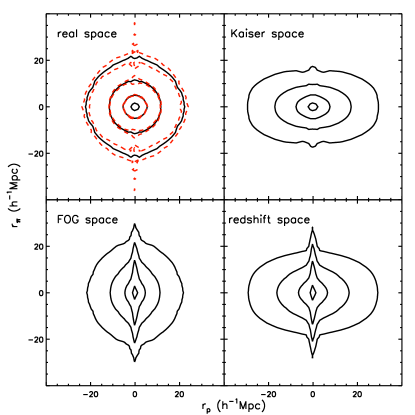
Figure 1.— The two-dimensional 2PCFs for mock galaxies with absolute $r$-band magnitudes in the range $-21\leq\>^{0.1}{\rm M}_{r}-5\log h\leq-20$ for four different spaces (see Table 2): real space (upper left), Kaiser space (upper right), FOG space (lower left) and redshift space (lower right). Black contours indicate the average values inferred from 10 mock samples. The contour levels correspond to $\xi=5,~{}1,~{}0.3,~{}0.1$. The red, dashed contours in the upper right-hand panel indicate the $\pm 1\sigma$ cosmic variance.

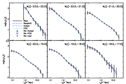
Figure 2.— Comparison of the projected two-point correlation functions in all seven mock spaces. Different panels correspond to different bins in absolute $r$-band magnitude, as indicated. For clarity, the error bars, which are obtained from the 10 mock samples, are only plotted for the real space results. Note that, as expected, all projected correlation functions are virtually indistinguishable.

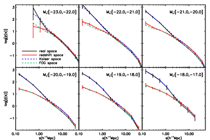
Figure 3.— The two-point correlation functions of mock galaxies in different true spaces. Results are shown for six different intervals in absolute $r$-band magnitude, as indicated. For clarity, we only plot error bars (expressing the variance among our 10 mock samples) for the real and redshift space results.

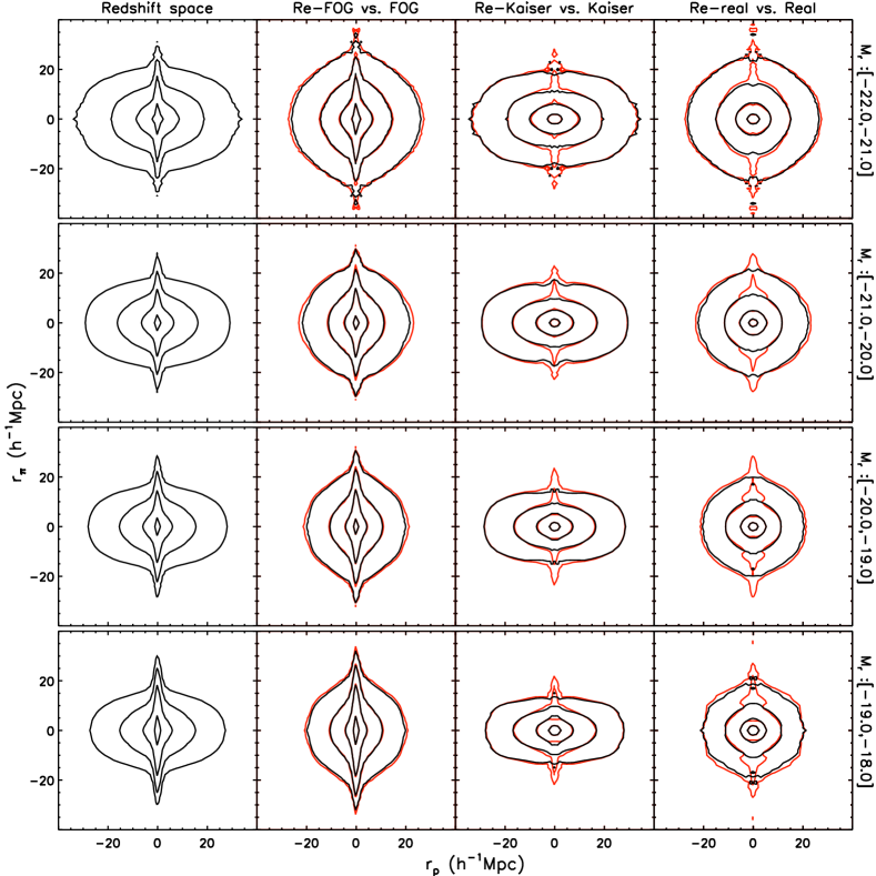
Figure 4.— Comparison of two-dimensional 2PCFs of mock galaxies. Different rows correspond to mock galaxies in different absolute $r$-band magnitude bins, as indicated at the right of each row. Different columns correspond to different spaces, as indicated at the top of each column. Black and red contours correspond to the results in the true and reconstructed spaces, respectively, with contour levels corresponding to $\xi=5,~{}1,~{}0.3,~{}0.1$.

Next, we proceed to construct mock galaxy samples that have the same survey selection effects as the SDSS DR7. We stack $3\times 3\times 3$ replicas of the populated simulation box and place a virtual observer at the center of central box. We define a $(\alpha,\delta)$ coordinate system, and remove all mock galaxies that are located outside of the SDSS DR7 survey region. We then assign each galaxy the redshift and $r$-band apparent magnitude according to its distance, line-of-sight velocity, and luminosity, and select galaxies according to the position-dependent magnitude limit. Finally, we mimic the position-dependent completeness by randomly sampling each galaxy using the completeness masks provided by the SDSS DR7. In order to have an rough estimation of the cosmic variance, we construct a total of 10 such mock samples by randomly rotating and shifting the boxes in the stack. Note that in order to get more accurate estimation of the cosmic variance, many more mocks are needed. From each mock sample, 6 flux limited (and volume limited) subsamples are constructed using the redshift and absolute magnitude ranges listed in Table 1.

Finally, in order to disentangle the various redshift distortions, for each mock galaxy redshift catalog we construct four different versions that only differ in the redshift $z_{\rm obs}$, assigned to each mock galaxy: a real-space version in which $z_{\rm obs}=z_{\rm cos}$, a Kaiser-space version in which $z_{\rm obs}=z_{\rm Kaiser}$ (Eq. [4]), a FOG-space version in which $z_{\rm obs}=z_{\rm FOG}$ (Eq. [5]), and a redshift-space version in which $z_{\rm obs}$ is given by Eq. (2).

4.2. Results for mock catalogs

In order to gauge the impact of the various redshift distortions, we now carry out clustering analyses of the various mock galaxy catalogs described above. We start our investigation by computing the two-dimensional 2PCF, $\xi(r_{\rm p},r_{\pi})$. Figure 1 shows the average results (black solid lines) from the 10 mock samples for the four true spaces. Here we only show the results for the $\bm{[}-21.0,-20.0\bm{]}$-subsample, but note that the results for the other subsamples are qualitatively very similar. The red dashes lines in the upper-left panel show the $\pm 1\sigma$ cosmic variance as inferred from our 10 mock samples. For enhanced clarity, we only show these in real space. Note that the variance causes small fluctuations at small transverse separations, $r_{\rm p}$, especially at larger line-of-sight separations, $r_{\pi}$.

Clearly, the shape of the two-dimensional correlation function is very different in different spaces: whereas $\xi(r_{\rm p},r_{\pi})$ is isotropic in real space, it is squashed along the line-of-sight on large scales in Kaiser space, and elongated along the line-of-sight on small scales in FOG space. Finally, in redshift space $\xi(r_{\rm p},r_{\pi})$ reveals the characteristics of both Kaiser and FOG space. All of this is well known since the seminal work by Davis & Peebles (1983).

Since redshift distortions only displace galaxies along the line-of-sight, they should not affect the projected correlation function, $w_{\rm p}(r_{\rm p})$, modulo RRSDs that arise from the use of a finite integration range (see discussion in §3.3). The lines in Fig. 2 show the projected 2PCFs in all four true spaces, and for all six absolute magnitudes bins: $\bm{[}-23.0,-22.0\bm{]}$, $\bm{[}-22.0,-21.0\bm{]}$, $\bm{[}-21.0,-20.0\bm{]}$, $\bm{[}-20.0,-19.0\bm{]}$, $\bm{[}-19.0,-18.0\bm{]}$, $\bm{[}-18.0,-17.0\bm{]}$. Error bars reflect the $\pm 1\sigma$ variance among the 10 mock samples, and, for clarity, are only plotted for the real space results (they are very similar in all other spaces). As expected, the various $w_{\rm p}(r_{\rm p})$ are in good agreement with each other, indicating that the impact of RRSDs is small compared to cosmic variance errors.

Finally, Fig. 3 shows the two-point correlation function, $\xi(s)$, for the same magnitude bins and the same four spaces. As before, error bars are obtained from the 10 mock samples, and only plotted for the real and redshift spaces for clarity. Unlike the projected correlation function, $\xi(s)$, clearly reveals the impact of redshift distortions. Compared to the real space correlation function, the $\xi(s)$ in Kaiser space is significantly boosted at large scales due to the large-scale flows toward over-dense regions (Kaiser effect). On small scales, however, the Kaiser space correlation function is virtually indistinguishable from the real space correlation function. The $\xi(s)$ in FOG space, on the other hand, is identical to the real space $\xi(s)$ on large scales, but dramatically suppressed on small scales. And finally, the $\xi(s)$ in redshift space clearly reveals redshift distortions from both the Kaiser effect and the FOG effect.

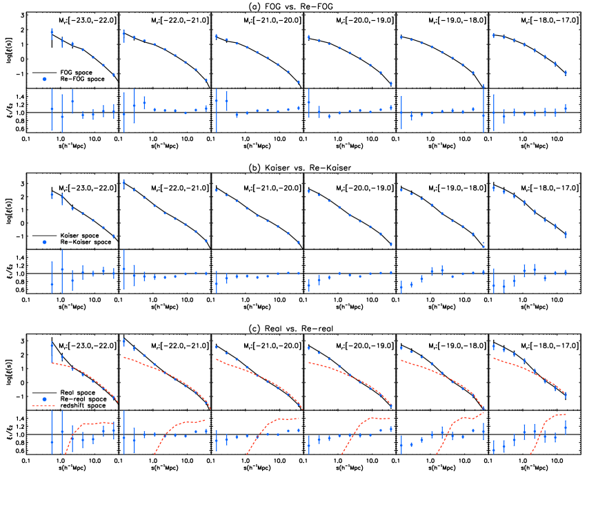
Figure 5.— 2PCFs (upper panels) and 2PCF ratios (lower panels) for mock galaxies in (a) FOG vs. re-FOG space, (b) Kaiser vs. re-Kaiser space and (c) real vs. re-real space. The solid line in the upper panels indicates the 2PCF in the true space, averaged over 10 mock samples, while the solid blue circles indicate the corresponding average 2PCF in the reconstructed space, with the error bars indicating the $\pm 1\sigma$ variance among the 10 mock samples. The lower panels plot the average and $\pm 1\sigma$ variance of the ratio of the 2PCFs in the reconstructed space over that in the true space. For comparison, the red dashed lines in the lower panels of (c) indicate the ratio of the redshift-space 2PCF to the true real space one. Different columns correspond to different $r$-band magnitude bins, as indicated.

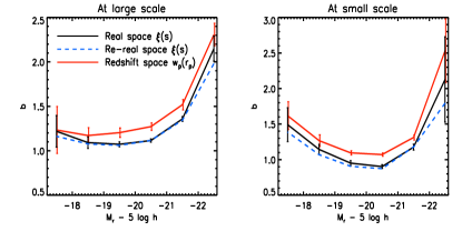
Figure 6.— The bias factor for mock galaxies as a function of galaxy absolute magnitude in real space (black solid lines), re-real space (blue dashed lines), and redshift space (red solid lines). The bias factors for real and re-real space are defined as the ratios of the measured $\xi(s)$ to that of the dark matter over the ranges of $4\>h^{-1}{\rm{Mpc}}<s<20\>h^{-1}{\rm{Mpc}}$ (left panel) and $0.5\>h^{-1}{\rm{Mpc}}<s<2\>h^{-1}{\rm{Mpc}}$ (right panel). The bias factor for redshift space is defined as the ratios of $w_{p}(r_{p})$ between galaxies and dark matter over the range $4\>h^{-1}{\rm{Mpc}}<r_{p}<20\>h^{-1}{\rm{Mpc}}$ (left panel) and $0.5\>h^{-1}{\rm{Mpc}}<r_{p}<2\>h^{-1}{\rm{Mpc}}$ (right panel). Here the integration limit, $r_{max}$, in computing $w_{p}(r_{p})$ from $\xi(r_{\rm p},r_{\pi})$, is set to be $60\>h^{-1}{\rm{Mpc}}$. The error bars, shown only for real space and redshift space, correspond to $1\sigma$ variance among 10 mock samples.

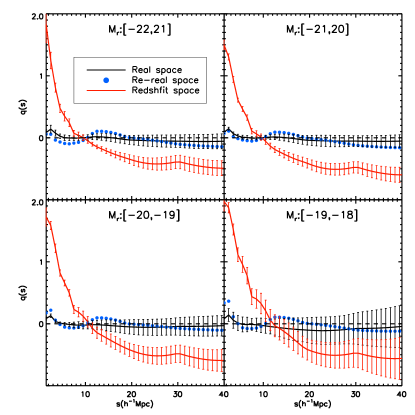
Figure 7.— The quadrupole-to-monopole ratio $q(s)$ for mock galaxies in real space (black solid lines), in reconstructed real space (blue solid circles) and in redshift space (red solid lines). Results indicate the averages obtained from 10 mocks, with error bars (for clarity, not plotted for re-real space) indicating the corresponding $\pm 1\sigma$ variance. Different panels correspond to different bins in absolute $r$-band magnitude, as indicated.

4.3. Results for reconstructed catalogs

Thus far we have constructed mock SDSS DR7 galaxy catalogs in four true spaces that allow us to disentangle the impact of the FOG effect on small scales from the Kaiser effect on large scales. We have shown that the results from statistical analyses of galaxy clustering in these different spaces agree with expectations. We now proceed with using these mock catalogs to test the reliability and accuracy of the reconstruction method described in §3.2. We start by running the halo-based group finder of Yang et al. (2005, 2007) over each of the separate true space mock galaxy catalogs. This yields corresponding mock group catalogs, in which each group is assigned a halo mass based on its characteristic luminosity, as described in Y07. Similar to the SDSS group catalog, the mock group catalogs are also complete to $z\sim 0.12$ for groups with an assigned halo mass $M_{\rm h}\geq 10^{12.5}\>h^{-1}\rm M_{\odot}$. We thus adopt a threshold mass of $M_{\rm th}=10^{12.5}\>h^{-1}\rm M_{\odot}$ and restrict our reconstruction to the volume covering the redshift range $0.01\leq z\leq 0.12$.

Next we use the redshift distortion correction method described in §3.2 to obtain mock galaxy catalogs in re-FOG, re-Kaiser and re-real space. In this subsection we focus on comparing the clustering of galaxies in the reconstructed spaces with that in the corresponding true spaces. The goal is to investigate the accuracy with which the reconstruction method can recover the distribution of galaxies in real space. Throughout we characterize the clustering using the various two-point correlation functions introduced above and we use the 10 independent mock samples to gauge the impact of sample variance.

4.3.1 The two-dimensional correlation function $\xi(r_{\rm p},r_{\pi})$

We start with a qualitative, visual comparison based on the two-dimensional 2PCF $\xi(r_{\rm p},r_{\pi})$. Different rows in Fig. 4 correspond to different magnitude bins, as indicated at the right-hand side of each row. From left to right, the different columns show the results in redshift space, a comparison of FOG vs. re-FOG, a comparison of Kaiser vs. re-Kaiser, and a comparison of real vs. re-real. In each case black and red contours correspond to the true and reconstructed spaces, respectively.

The $\xi(r_{\rm p},r_{\pi})$ in redshift space is clearly anisotropic, revealing fingers-of-God on small scales and the impact of the Kaiser effect on large scales. After correcting for the Kaiser effect, the resulting $\xi(r_{\rm p},r_{\pi})$ in re-FOG space is clearly more isotropic on large scales. As expected, it still reveals the impact of the FOG effect, which distort the contours from being perfectly round. A comparison with the $\xi(r_{\rm p},r_{\pi})$ in FOG space shows that the correction for the Kaiser effect is overall very successful, except for small differences in the outer contour (corresponding to $\xi=0.1$).

Comparing the $\xi(r_{\rm p},r_{\pi})$ in re-Kaiser space (third column from the left) with that in redshift space (left-hand column) shows that our method of FOG compression is fairly accurate. However, a comparison with the true Kaiser space results (black contours in third column) reveals that the method is not perfect. On small scales, the $\xi(r_{\rm p},r_{\pi})$ in re-Kaiser space shows very nice agreement with that in the real space. On large scales, however, the correlation function in re-Kaiser space reveals residual FOG effects. These shortcomings of the FOG compression may arise from problems with the group finder, including errors in group membership determination (‘fracturing’ and ‘fusing’ of groups), errors in the designation of centrals and satellites, and errors in the halo mass assignment. These errors are characteristic of all group finders, and are virtually impossible to avoid (see Campbell et al., 2015, for details).

Finally, the results in the rightmost column show that the reconstruction of $\xi(r_{\rm p},r_{\pi})$ in real space manifests both the problems with the Kaiser correction and the FOG compression. Overall, though, comparing the correlation function in re-real space with that in redshift space, it is clear that the reconstruction method has successfully corrected for the majority of redshift space distortions. In order to make this more quantitative, we now focus on $\xi(s)$.

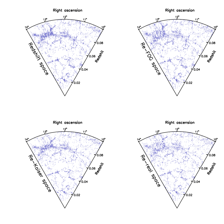
Figure 8.— Distribution of a subset of SDSS DR7 galaxies in a $4^{\circ}$ slice with right ascensions in the range from $14^{{\rm h}}$ to $10^{{\rm h}}$ and with redshifts $0.01\leq z\leq 0.1$. Clockwise from the top-left, the panels show results in redshift space, in reconstructed FOG space, in reconstructed real space, and in reconstructed Kaiser space. Note how the Sloan Great Wall, evident in the upper left corner of each panel, is far less pronounced in real space than in redshift space.

4.3.2 The one-dimensional correlation function $\xi(s)$

Figure 5 compares the 2PCF, obtained by averaging results from all 10 mocks, in a true space ($\xi_{\rm true}$, solid lines) to that in the corresponding reconstructed space ($\xi_{\rm recon}$, blue filled circles). From top to bottom, the three parts of this figure show a comparison of (a) FOG space versus re-FOG space, (b) Kaiser space versus re-Kaiser space, and (c) real space versus re-real space. Different columns correspond to different magnitude bins, as indicated, and error bars indicate the variance among the 10 mock samples. In each part, the upper panels show the actual 2PCFs, while the lower panels plot $\xi_{\rm recon}/\xi_{\rm true}$. Overall, the correlation functions in the reconstructed spaces are in excellent agreement with those in their corresponding true spaces, with the vast majority of data points being consistent with $\xi_{\rm recon}/\xi_{\rm true}=1$ within $1\sigma$. Recall that $\sigma$ reflects the measurement error due to cosmic variance in a SDSS-like survey.

As is evident from the middle part (b), the FOG compression seems to systematically under predict the Kaiser-space 2PCF for faint galaxies. The effect, which results from inaccuracies in the group finder, is somewhat significant in the two low mass bins. Thus in an accurate modeling for the halo occupation distribution of galaxies for these faint galaxies, one needs to taken this effect into account. For brighter galaxies, over the range of scales $0.2\leq(s/\>h^{-1}{\rm{Mpc}})\leq 20$, the average values of $\xi_{\rm re-real}/\xi_{\rm real}$ is $1.00\pm 0.050$. Hence, we conclude that over those scales the reconstruction of the real space correlation function is accurate at five percent level. For comparison, the dashed lines in the bottom part (c) of Fig. 5 correspond to the 2PCF in redshift space. On small scales ($r<1\>h^{-1}{\rm{Mpc}}$), the clustering strength in redshift space is suppressed by $\sim 70\%$ on average, compared to that in real space. On large scales, ($r>2\>h^{-1}{\rm{Mpc}}$) it is boosted by $\sim 30\%$ on average.

4.3.3 The projected correlation function $w_{\rm p}(r_{\rm p})$

Moreover, since our reconstruction only ‘displaces’ galaxies along the line-of-sight, the reconstruction method has no impact on the projected correlation function, $w_{\rm p}(r_{\rm p})$, other than scattering a few galaxy pairs in and out of the sample due to the finite integration range used ($|r_{\pi}|\leq 100\>h^{-1}{\rm{Mpc}}$). This effect is entirely negligible, though, as is evident from Fig. 2, which shows the results for all of our seven spaces (four true space and three reconstructed spaces). There are no significant differences among these different projected correlation functions.

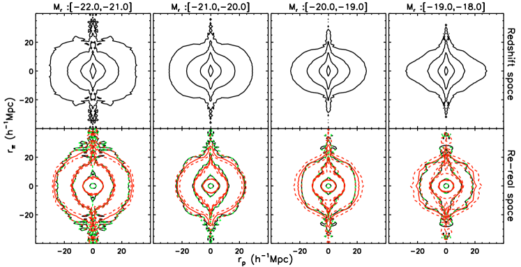
Figure 9.— The two-dimensional 2PCFs for SDSS DR7 data in redshift space (upper panels) and re-real space (lower panels). Different columns correspond to different magnitude bins as indicated. The black solid lines in the lower panels are for WMAP9 cosmology, and the green dashed lines are for Planck cosmology. The red, solid and dashed contours indicate the average and $\pm 1\sigma$ variance, respectively, obtained from the 10 mock galaxy samples in re-real space. Contour levels correspond to $\xi=5,~{}1,~{}0.3,~{}0.1$.

4.3.4 The bias factor

The correlation function of galaxies relative to that of dark matter is usually described by a bias factor, which is defined

$$\xi_{gg}(s)=b^{2}\xi_{mm}(s)\,,$$ (25)

where $\xi_{gg}$ and $\xi_{mm}$ are the correlation functions of galaxies and mass, respectively. In general, the bias factor $b$ may depend on $s$. Figure 6 shows the best-fitting bias factor, as a function of galaxy luminosity, obtained from the measured $\xi(s)$ for mock galaxies relative to the correlation function of dark matter at $z=0.1$. The real-space and reconstructed real-space $b$ shown in the left panel are obtained from using the values of $\xi(s)$ at large scales, $4\>h^{-1}{\rm{Mpc}}<s<20\>h^{-1}{\rm{Mpc}}$, while in the right panels they are obtained using the correlation functions on small scales, $0.5\>h^{-1}{\rm{Mpc}}<s<2\>h^{-1}{\rm{Mpc}}$. For comparison, we also show in Figure 6 the bias factor based on the projected 2PCFs (red lines), defined as the ratios of $w_{p}(r_{p})$ between galaxies and dark matter over the range $4\>h^{-1}{\rm{Mpc}}<r_{p}<20\>h^{-1}{\rm{Mpc}}$ (left panel) and $0.5\>h^{-1}{\rm{Mpc}}<r_{p}<2\>h^{-1}{\rm{Mpc}}$ (right panel). As one can see, the reconstructed real-space $b$ closely matches that in the real-space, while the traditional method based on $w(r_{p})$ leads to larger errors and biased results relative to the true real-space values.

4.3.5 The quadrupole-to-monopole ratio $q(s)$

As a final diagnostic of our reconstruction performance, we consider the quadrupole-to-monopole ratio, which is defined as

$$q(s)\equiv\frac{\xi_{2}(s)}{\frac{3}{s^{3}}\int^{s}_{0}{\xi_{0}(s^{\prime})\,s^{\prime 2}\,{\rm d}s^{\prime}}-\xi_{0}(s)}$$ (26)

with $\xi_{l}(s)$ given by

$$\xi_{l}(s)=\frac{2l+1}{2}\int^{1}_{-1}{\xi(r_{\rm p},r_{\pi})\,\mathscr{P}_{l}(\mu)\,{\rm d}\mu}$$ (27)

where $\mathscr{P}_{l}(\mu)$ is the $l$th Legendre polynomial. In redshift space, the Kaiser effect causes the quadrupole-to-monopole ratio to become negative on large scales, asymptoting towards

$$q(s)={-{4\over 3}\beta-{4\over 7}\beta^{2}\over 1+{2\over 3}\beta+{1\over 5}\beta^{2}}\,,$$ (28)

where $\beta=f(\Omega)/b$ with $b$ the bias parameter of the galaxy population under consideration (e.g., Hamilton, 1992; Cole et al., 1994). On small scales the FOG effect causes $q(s)$ to become positive. In real space, however, we expect isotropy to results in a quadrupole $\xi_{2}(s)=0$. Hence, if the correction for redshift distortions is successful, the resulting clustering should have a vanishing quadrupole, and thus $q(s)=0$.

Figure 7 shows the quadrupole-to-monopole ratio in our real space, re-real space and redshift space mocks. Different panels correspond to different magnitude bins, as indicated. As expected, in redshift space $q(s)$ has large deviations from zero on both small and large scales, while in real space $q(s)$ is close to zero (except for a small positive signal for $r\lower 3.01385pt\hbox{$\;\buildrel<\over{\sim}\;$}3\>h^{-1}{\rm{Mpc}}$, which is due to noise). In re-real space, the quadrupole-to-monopole ratio in the re-real space is consistent with zero within the error bars on large scales ($\lower 3.01385pt\hbox{$\;\buildrel>\over{\sim}\;$}12\>h^{-1}{\rm{Mpc}}$). On smaller scales, all magnitude bins reveal a slightly negative $q(s)$. This is a consequence of the over-correction for the FOG effect on small scales discussed in §4.3.1 (cf. Fig. 4), which has its origin in inaccuracies associated with the galaxy group finder.

5. APPLICATION TO THE SLOAN DIGITAL SKY SURVEY

Based on the analyses of the mock galaxy samples discussed in §4, we conclude that our reconstruction method can accurately correct for redshift space distortions in a statistical sense. In this section we apply exactly the same method to the SDSS DR7. As described in §2 we follow W12 and reconstruct the velocity field on quasi-linear scales using the mass distribution reconstructed from galaxy groups of Y07 in the redshift range $0.01\leq z\leq 0.12$ and with assigned halo masses $\log(M_{\rm h}/\>h^{-1}\rm M_{\odot})\geq 12.5$. We use the velocities derived to correct for the Kaiser effect using the method described in §3.2.1. Finally, we correct for the FOG effect by assigning all galaxies new positions within their groups based on the method described in §3.2.2. We apply this method to all the 396,068 galaxies in the NGC region. The reconstructed real space galaxy catalog is publicly available through http://gax.shao.ac.cn/data/data1/SDSS7_REAL.tar.

5.1. The galaxy distribution

To visualize the effects of our reconstruction method on galaxy distribution, we shown in Fig. 8 the distributions of galaxies with declination $|\delta|<4^{\circ}$, right ascensions $10^{\rm h}\leq\alpha\leq 14^{\rm h}$, and redshifts $0.01\leq z\leq 0.1$. The four different panels show the galaxy distributions in redshift space (upper-left panel), re-FOG space (upper-right panel), re-Kaiser space (lower-left panel), and re-real space (lower-right panel), respectively. Note that the volume chosen includes the Sloan Great Wall, which is readily visible in the upper left corner ($z\sim 0.085$ and $12^{\rm h}\leq\alpha\leq 14^{\rm h}$).

There are a few noteworthy trends. First of all, the prominent ‘finger’ structures clearly visible in redshift space are no longer visible in the re-Kaiser space, indicating that our FOG compression is successful. Comparing the redshift space distribution with that in re-real space, one sees that the distribution in re-real space appears more diffused on large scales, more compressed on small scales. In particular, the Sloan Great Wall is clearly much broader, and thus less pronounced, in the re-FOG and re-real spaces. This suggests that the Sloan Great Wall is not as dominant an over-dense structure as it appears to be in redshift space, but that its apparent over-density is strongly enhanced by the Kaiser effect.

It is also clear from Fig. 8 that some geometrical properties of the large scale structure may also be affected as one goes from real space to redshift space distortion. For example, the voids appear to be smaller and the filamentary structures less prominent in real space. Clearly, detailed analyses are needed in order to quantify the effects, and our reconstructed real-space catalog of SDSS DR7 provides a unique resource for such studies.

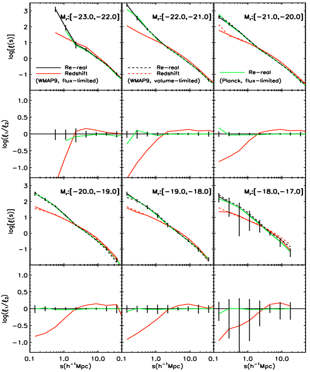
Figure 10.— The 2PCFs and 2PCF ratios for SDSS galaxies in redshift space (red lines) and the reconstructed real space ( WMAP9 with black lines, Planck with green lines). For comparison, the 2PCFs of the flux-limited (solid lines) and volume-limited samples (dashed lines) are both shown. Error bars, only shown for the re-real space results, are the $\pm 1\sigma$ variance among the 10 mock samples discussed in §4.1. The red curves in the lower panels are the ratios of the redshift space to re-real space 2PCFs. Different columns correspond to different bins in absolute $r$-band magnitude, as indicated.

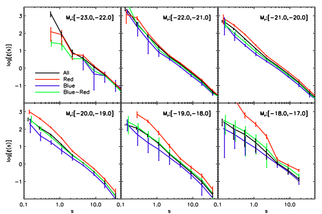
Figure 11.— The 2PCFs of red and blue galaxies for SDSS volume-limited samples in re-real space. Different columns correspond to different bins in the absolute $r$-band magnitude, as indicated. Red and blue lines show the autocorrelation functions of the red and blue subsamples, respectively, while black lines show the autocorrelation of the full sample in each $M_{r}$ bin. Green lines show the cross-correlation function between red and blue galaxies.

[c] $~{}~{}~{}~{}~{}\bm{[}-23,~{}-22\bm{]}$ $~{}~{}\bm{[}-22,~{}-21\bm{]}$ $~{}~{}~{}~{}~{}\bm{[}-21,~{}-20\bm{]}$ $~{}~{}\bm{[}-20,~{}-19\bm{]}$ $\bm{[}-19,~{}-18\bm{]}$ $\bm{[}-18,~{}-17]\bm{}$   $r$    $\xi(\xi^{\prime})$    $\mathop{\Delta\xi}$    $\xi(\xi^{\prime})$    $\mathop{\Delta\xi}$   $\xi$   $\xi^{\prime}$    $\mathop{\Delta\xi}$   $\xi$   $\xi^{\prime}$    $\mathop{\Delta\xi}$   $\xi$   $\xi^{\prime}$    $\mathop{\Delta\xi}$   $\xi$   $\xi^{\prime}$    $\mathop{\Delta\xi}$ 0.14 113.849 34.734 59.898 134.516 14.312 47.269 36.029 6.318 38.225 46.719 12.109 22.684 40.278 19.146 Redshift space 0.28 49.288 8.310 30.435 25.849 2.486 25.203 24.042 1.322 20.512 24.432 1.770 21.377 20.144 4.651 0.56 42.401 22.572 23.400 1.410 15.645 17.469 0.730 14.101 14.980 0.519 13.083 12.962 0.954 12.261 11.008 3.446 1.12 19.626 10.093 11.659 0.382 8.686 8.670 0.231 7.078 7.234 0.226 6.540 6.643 0.356 5.915 6.134 1.894 2.24 9.474 4.009 5.424 0.136 4.070 4.044 0.086 3.313 3.275 0.097 3.070 3.174 0.225 3.067 3.298 0.918 4.47 5.308 0.645 2.191 0.055 1.750 1.730 0.034 1.479 1.423 0.047 1.346 1.392 0.117 1.339 1.504 0.406 8.91 1.516 0.090 0.773 0.032 0.652 0.646 0.022 0.539 0.488 0.030 0.470 0.483 0.062 0.450 0.598 0.195 17.78 0.458 0.058 0.221 0.022 0.190 0.187 0.014 0.137 0.114 0.020 0.116 0.122 0.024 0.083 0.190 0.046 35.48 0.109 0.023 0.055 0.007 0.048 0.051 0.006 0.028 0.021 0.006 0.024 0.018 0.008 0.14 1386.112 517.165 401.879 496.315 63.661 314.918 372.194 75.121 315.778 178.442 52.512 203.865 267.397 113.507 Re-real space 0.28 403.161 91.274 145.658 178.764 17.368 137.039 118.726 18.983 112.085 112.744 16.460 85.958 100.588 74.667 0.56 1308.251 425.252 82.973 9.812 49.341 47.769 3.154 49.473 49.278 3.563 44.412 44.125 8.146 40.043 49.205 39.238 1.12 90.370 27.875 16.178 1.398 13.415 13.065 0.705 13.028 13.050 0.905 13.116 14.809 3.118 13.187 16.850 11.799 2.24 7.865 3.316 4.576 0.161 3.757 3.721 0.132 3.248 3.237 0.229 3.321 3.732 0.687 3.799 4.501 2.614 4.47 3.645 0.730 1.737 0.051 1.386 1.384 0.028 1.164 1.162 0.037 1.092 1.103 0.071 0.996 1.116 0.232 8.91 1.175 0.125 0.567 0.027 0.478 0.471 0.015 0.385 0.359 0.019 0.342 0.330 0.048 0.303 0.431 0.153 17.78 0.413 0.034 0.180 0.017 0.152 0.150 0.012 0.110 0.090 0.016 0.097 0.095 0.021 0.069 0.137 0.035 35.48 0.105 0.019 0.044 0.006 0.037 0.039 0.005 0.021 0.015 0.005 0.023 0.018 0.005 Notes. $r$: the comoving distances in units of $\>h^{-1}{\rm{Mpc}}$.  $\xi$: the two-point correlation function for flux limited samples.  $\xi^{\prime}$: the two-point correlation function for volume-limited samples (the flux- and volume- limited samples are the same for the first two samples).   $\mathop{\Delta\xi}$: the $1\sigma$ error of $\xi(s)$ estimated using 10 mock samples.

Table 3The 2PCFs obtained from SDSS DR7 in redshift space and reconstructed real space.

5.2. The clustering of galaxies

Next we investigate the galaxy clustering properties. It is important to note that the reconstruction to obtain the re-real space is cosmology dependent. The bias parameter $b$, the halo mass assignments to galaxy groups, and the distance-redshift relation are all cosmology dependent. In the reconstruction of the SDSS-DR7, we have adopted the cosmological parameters as inferred from the WMAP9. To check the impact of cosmology on our results, we also adopt a Planck cosmology ($\Omega_{\rm m}=0.308$, $\Omega_{\Lambda}=0.692$, $n_{\rm s}=0.968$, $h=H_{0}/(100\>{\rm km}\,{\rm s}^{-1}\,{\rm Mpc}^{-1})=0.678$ and $\sigma_{8}=0.815$) (Planck Collaboration et al., 2015) in our reconstruction. In general, there is no large distinction between the results for the two cosmologies. In what follows, we mainly focus on the results for the WMAP9 cosmology, results for Planck cosmology are also presented where necessary.

The black contours in Fig. 9 show the two dimensional 2PCFs $\xi(r_{\rm p},r_{\pi})$, for galaxies in four luminosity bins, in redshift space (upper panels) and re-real space (lower panels) for WMAP9 cosmology. While the green contours are results for Planck cosmology, which show quite good agreement with those for WMAP9 cosmology. After the correction of the redshift distortion, the $\xi(r_{\rm p},r_{\pi})$ is clearly much more isotropic than in redshift space. However, it is also clear that the correction is not perfect, especially on small transverse scales where residual deviations from isotropy are apparent. To assess the significance of these deviations, we use the 10 mock re-real space samples of §4.3 to estimate the significance of the cosmic variance. The solid and dashed red contours in the lower panels of Fig. 9 show the average and $\pm 1\sigma$ variance among these 10 mock samples. Clearly, the variance is large, and most of the black contours fall within these $1\sigma$ error ranges, suggesting that the remaining deviations from isotropy are mainly a manifestation of sampling variance, rather than a systematic error in the reconstruction method.

[c] $~{}~{}~{}~{}~{}\bm{[}-23,~{}-22\bm{]}$ $~{}~{}\bm{[}-22,~{}-21\bm{]}$ $~{}~{}~{}~{}~{}\bm{[}-21,~{}-20\bm{]}$ $~{}~{}\bm{[}-20,~{}-19\bm{]}$ $\bm{[}-19,~{}-18\bm{]}$ $\bm{[}-18,~{}-17]\bm{}$   $r$    $\xi$    $\mathop{\Delta\xi}$    $\xi$    $\mathop{\Delta\xi}$   $\xi$    $\mathop{\Delta\xi}$   $\xi$    $\mathop{\Delta\xi}$   $\xi$    $\mathop{\Delta\xi}$   $\xi$    $\mathop{\Delta\xi}$ 0.14 1771.494 367.491 429.502 348.935 218.154 154.158 213.160 134.140 108.841 106.506 0.28 240.858 171.663 70.223 31.927 42.708 20.893 50.913 39.207 51.447 43.761 Blue Galaxies 0.56 40.259 33.505 20.414 2.658 17.686 4.379 16.873 12.391 19.772 16.476 1.12 8.188 3.437 6.342 1.239 5.974 2.135 6.896 5.297 8.139 3.767 2.24 3.336 0.445 2.458 0.219 2.162 0.511 2.357 1.391 2.791 0.206 4.47 3.294 2.496 1.185 0.062 0.963 0.036 0.846 0.054 0.820 0.167 0.993 0.343 8.91 0.461 0.407 0.376 0.050 0.323 0.022 0.257 0.034 0.244 0.100 0.363 0.108 17.78 0.369 0.217 0.129 0.027 0.104 0.018 0.064 0.021 0.061 0.045 0.109 0.041 35.48 0.122 0.076 0.035 0.007 0.029 0.007 0.010 0.013 0.011 0.015 0.14 1203.324 828.281 726.580 387.987 1000.507 237.858 267.370 552.352 0.28 741.101 152.922 288.323 28.802 400.555 33.271 717.431 262.018 5641.724 467.787 Red Galaxies 0.56 122.181 87.634 99.281 11.245 85.996 4.259 125.857 7.515 286.505 47.521 643.570 213.487 1.12 83.521 61.860 20.250 1.187 20.914 1.245 30.289 2.238 61.773 14.289 193.317 49.260 2.24 6.535 3.474 5.244 0.301 5.073 0.261 5.543 0.408 11.068 2.652 38.960 9.931 4.47 5.235 0.688 2.000 0.077 1.771 0.039 1.717 0.051 2.063 0.215 1.801 0.494 8.91 1.344 0.156 0.666 0.032 0.613 0.023 0.544 0.030 0.660 0.111 0.866 0.123 17.78 0.463 0.060 0.209 0.020 0.196 0.017 0.135 0.020 0.218 0.048 0.431 0.066 35.48 0.119 0.033 0.051 0.006 0.050 0.007 0.025 0.013 0.035 0.015 0.14 7239.943 1692.040 378.739 171.435 395.622 151.954 298.611 245.189 331.254 278.698 0.28 322.883 113.649 102.018 22.364 108.949 25.905 141.057 71.610 159.180 139.079 0.56 29.292 11.156 70.285 6.320 31.018 2.973 36.225 4.991 46.072 27.418 72.262 69.431 Blue-Red 1.12 24.140 12.885 11.180 2.338 9.037 1.147 10.487 2.172 16.782 14.033 25.419 21.754 2.24 3.424 5.895 3.949 0.280 3.086 0.235 3.076 0.455 4.082 2.574 7.629 6.999 4.47 3.477 0.747 1.525 0.060 1.200 0.034 1.178 0.052 1.291 0.189 1.404 0.413 8.91 0.701 0.244 0.485 0.032 0.388 0.021 0.365 0.031 0.395 0.106 0.627 0.112 17.78 0.371 0.062 0.155 0.022 0.102 0.016 0.092 0.020 0.120 0.046 0.215 0.050 35.48 0.100 0.033 0.038 0.007 0.004 0.007 0.014 0.012 0.021 0.014 Notes. Here $r$ is the comoving distances in units of $\>h^{-1}{\rm{Mpc}}$;   $\xi$ is the two-point correlation function for a volume limited sample;   $\mathop{\Delta\xi}$ is the $1\sigma$ error of $\xi(s)$ estimated from 10 mock samples;  The auto-correlations of blue and red galaxies, and the cross-correlations between blue and red galaxies, are shown in the upper, middle, and lower parts, respectively.

Table 4The color-dependence of the 2PCF measured from SDSS DR7 in the reconstructed real space.

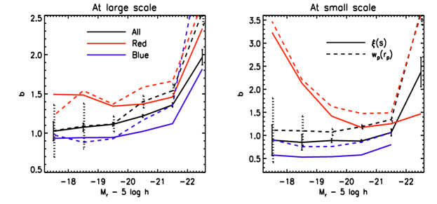
Figure 12.— The bias factor for SDSS DR7 galaxies as a function of galaxy absolute magnitude. Solid lines show the bias factors defined as the ratios of the measured reconstructed real-space $\xi(s)$ to that of dark matter over the ranges of $4\>h^{-1}{\rm{Mpc}}<s<20\>h^{-1}{\rm{Mpc}}$ (left panel) and $0.5\>h^{-1}{\rm{Mpc}}<s<2\>h^{-1}{\rm{Mpc}}$ (right panel). Dashed lines show the bias factors defined by the ratios of $w_{p}(r_{p})$ between the redshift-space galaxies and dark matter over the ranges of $4\>h^{-1}{\rm{Mpc}}<r_{p}<20\>h^{-1}{\rm{Mpc}}$ (left panel) and $0.5\>h^{-1}{\rm{Mpc}}<r_{p}<2\>h^{-1}{\rm{Mpc}}$ (right panel). Here the integration limit, $r_{max}$, in computing $w_{p}(r_{p})$ from $\xi(r_{\rm p},r_{\pi})$, is set to be $60\>h^{-1}{\rm{Mpc}}$. Black, red and blue lines show results for all, red and blue galaxies, respectively. Error bars obtained from 10 mock samples are shown only for black solid and dashed lines.

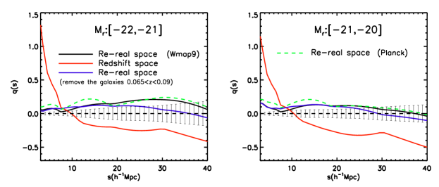
Figure 13.— The quadrupole-to-monopole ratio $q(s)$ for SDSS DR7 galaxy subsamples in the $r$-band absolute magnitude bin $M_{r}=$ $\bm{[}-22.0,-21.0\bm{]}$, $\bm{[}-21.0,-20.0\bm{]}$, as indicated. Black and red lines correspond to the results in redshift and re-real spaces (WMAP9), respectively. Blue lines are results in the re-real spaces in which galaxies with $0.065\leq z\leq 0.09$ are removed to check the impact of the Sloan Great Wall. The results for the Planck cosmology are shown with green dashed lines. The error bars are $1\sigma$ variances obtained from 10 mock re-real space samples. The dashed lines are the zero reference line.

Fig. 10 shows the one-dimensional 2PCFs in redshift space (red lines) and in re-real space (black lines) for WMAP9 cosmology, for all the six magnitude samples, as indicated. While the green lines are results for Planck cosmology, here again show very good agreement with those for WMAP9 cosmology. For comparison, the results of both the flux-limited and volume-limited samples are shown. Note that for the two brightest samples, flux-limited and volume limited samples are identical. For the other samples, the correlation functions obtained from the two types of samples are very similar, even though the samples themselves are quite different, especially for the faint magnitude bins (see Table 1). Error bars for the real space correlation function indicate the $\pm 1\sigma$ variance among the 10 re-real mock samples described in §4. All the results shown in the figure are also listed in Table 3. To our knowledge, this is the first attempt to infer the real-space correlation function of galaxies in the SDSS directly from a reconstructed real space galaxy catalog. Note that the real space 2PCFs clearly deviate from a simple, single power-law, revealing a clear 1-halo to 2-halo transition on scales of $1-3\>h^{-1}{\rm{Mpc}}$. As demonstrated in §4, this transition is more pronounced in real space than in the projected space. It is, therefore, expected that fitting halo occupation models directly to the real space correlation functions presented here will provide more stringent constraints on the galaxy-dark matter halo connection, something we will pursue in a forthcoming paper. Finally, the lower panels of Fig. 10 show the ratio $\xi_{1}/\xi_{2}$, where $\xi_{1}(s)$ and $\xi_{2}(s)$ are the two-point correlation functions in redshift space and re-real space, respectively. This nicely shows how redshift space distortions boost the correlation power on large scales (by about $40-50\%$ at a scale of $10\>h^{-1}{\rm{Mpc}}$), while suppressing it on small scales (by about $70-80\%$ at a scale of $0.3\>h^{-1}{\rm{Mpc}}$).

To study how galaxy clustering depends on galaxy color, we use the bimodal distribution in the color-magnitude plane (e.g. Strateva et al., 2001; Baldry et al., 2004) to divide each of the luminosity samples into “blue” and “red” subsamples. Specifically, the demarcation line we use is $(g-r)=0.21-0.03M_{r}$, as is in Zehavi et al. (2011). Information about these subsamples is given in Table 1.

Figure 11 shows the 2PCFs of red (red lines) and blue galaxies (blue lines) in re-real space for different magnitude bins, as indicated. The result of the full sample in each magnitude bin is also shown in each panel as black line. Green lines show the cross-correlation functions between blue and red galaxies. The cross-correlation is obtained by replacing $\langle DD\rangle$, $\langle RR\rangle$ and $\langle DR\rangle$ with $\langle D_{1}D_{2}\rangle$, $\langle R_{1}R_{2}\rangle$ and $(\langle D_{1}R_{2}\rangle+\langle D_{2}R_{1}\rangle)/2$, respectively, in Equation 13. Here subscripts ‘1’ and ‘2’ denote red and blue galaxies, respectively, so that $D_{1}D_{2}$ is the number of cross pairs between red and blue galaxies, and so on. Error bars are obtained from the 10 mock samples. All the data shown in this plot are also listed in Table 4 for references. As one can see, red galaxies exhibit higher clustering amplitude than the blue ones in the same luminosity bin, and the cross-correlation lies in between. The difference between red and blue galaxies appears to be larger for fainter galaxies.

Figure 12 shows the bias factors defined in the same way as those in Figure 6. Solid lines in the left panel show the bias factors obtained from using the values of $\xi(s)$ at large scales, $4\>h^{-1}{\rm{Mpc}}<s<20\>h^{-1}{\rm{Mpc}}$, while in the right panels, the same type of lines show the bias factors obtained by using data on small scales, $0.5\>h^{-1}{\rm{Mpc}}<s<2\>h^{-1}{\rm{Mpc}}$. Black, red and blue lines show the results for all, red and blue galaxies in each $M_{r}$ bin, respectively. Clearly, the bias factor depends on galaxy luminosity, but the dependence is not in the same way for red and blue galaxies. Overall, red galaxies have a higher bias factor than their blue counterparts in the same luminosity bin. The difference is the largest for faint galaxies on small scales. For the total and blue populations, the bias factor on large scales increases with luminosity. In contrast, for red galaxies, the bias factor on large scales remains more or less constant all the way to $M_{r}-5\log h\sim-21.5$, and only increases with luminosity for the brightest galaxies. On small scales, the bias factor is quite independent of luminosity for both the total and blue populations at $M_{r}-5\log h>-20.5$, and increases with luminosity for higher luminosities. In contrast, the bias factor for red galaxies decreases with increasing luminosity, especially for faint galaxies. This indicates that faint red galaxies are preferentially satellites located in relatively big halos, consistent with the results of Lan et al. (2016) based on the luminosity functions of galaxies in groups.

For comparison, the dashed lines in Figure 12 shows the bias parameters obtained from the projected 2PCFs, $w_{p}(r_{p})$, again estimated in the same way as those for mock galaxies (see Figure 6). The results show again that the bias parameter, $b$, estimated from the projected 2PCF has larger errors and is biased relative to that obtained from the reconstructed real-space $\xi(s)$, as is demonstrated using mock samples shown in Figure 6. This suggests that the bias parameters obtained earlier in the literature on the basis of $w_{p}(r_{p})$ may be significantly biased. We will come back to a detailed analysis on this in a forthcoming paper.

Finally, we compute the quadrupole-to-monopole ratio $q(s)$ for the SDSS DR7 galaxies. Figure 13 shows the $q(s)$ for two luminosity samples, $M_{r}=[-22.0,-21.0]$ and $[-21.0,-20.0]$, respectively. In each panel, results are shown for galaxies in both redshift and re-real spaces using lines with different colors. as indicated. The error bars on top of the zero line correspond to $1\sigma$ variances obtained from 10 mock samples in re-real space. We see that $q(s)$ in re-real space in SDSS DR7 has a systematic deviation from the zero line at 2-$\sigma$ level, especially for the high-luminosity bin. This deviation may indicate that at $z\leq 0.12$ the SDSS DR7 volume still suffers from cosmic variance, likely produced by the existence of rare large-scale structures, such as the Sloan Great Wall. To check this we estimate $q(s)$ excluding galaxies with redshifts $0.065\leq z\leq 0.09$, which effectively excludes the Sloan Great Wall. The results are shown in Figure 13 as the blue lines. The deviations from the zero line are significantly reduced at large $s$. This test result suggests that the quadrupole-to-monopole ratio is sensitive to the presences of large scale structures, and a much larger volume is required to get a reliable estimate of this quantity.

On the other hand, as discussed at the beginning of this subsection, the reconstruction to obtain the re-real space distribution of galaxies is cosmology dependent. If the real universe deviates from the assumed cosmology, systematic errors can also be introduced in our reconstruction. The $q(s)$ for Planck cosmology, which are shown in Figure 13 as the green dashed lines, do show some differences from those for the WMAP9 cosmology. After the removal of the Sloan Great Wall, the deviation of $q(s)$ from zero is about $0.1$ at $s\sim 20\>h^{-1}{\rm{Mpc}}$. This corresponds to an under-estimate of $\beta$ by about $0.07$ in the linear regime by WMAP9. We will perform a detailed cosmological probe in a follow-up paper.

6. SUMMARY

We have presented a method to correct redshift space distortions in redshift surveys of galaxies. Adopting the method introduced in W12, we use galaxy groups identified with the Y05 halo-based group finder to reconstruct the large scale velocity field, which in turn is used to correct the observed redshifts for the Kaiser effect. The same galaxy groups are also used to correct the Finger-Of-God (FOG) effect produced by the virial motions of galaxies within their host dark matter halos. Our FOG correction is based on the assumption that satellite galaxies are an unbiased tracer of the mass profile and velocity structure of the host halo.

To test the method, we have constructed 10 mock SDSS DR7 galaxy catalogs, in four different spaces: redshift space (equivalent to the observational space), Kaiser space (space in which the FOG effect is absent), FOG space (space in which Kaiser effect if absent), and real space (space in which redshift distortions are absent). We test the various components of our reconstruction method by comparing the two-point clustering statistics in these different spaces.

The contours of the two-dimensional 2PCFs $\xi(r_{\rm p},r_{\pi})$ calculated in different spaces show that the clustering in our reconstructed space is in good agreement with that in the corresponding true space given directly by numerical simulations. On small transverse scales $r_{\rm p}$, residual FOG effects are apparent, which arise mainly from the uncertainties in the group finder, including errors in group membership determinations, designations of centrals and satellites, and halo mass assignments. We have shown, though, that the one-dimensional 2PCF, $\xi(s)$, inferred directly from the reconstructed real space is not significantly affected, with deviations typically being smaller than the uncertainties arising from cosmic variance (at least for a SDSS-like survey) for galaxies brighter than $\>{}^{0.1}{\rm M}_{r}-5\log h=-19.0$. In fact, over the range of scales $0.2\>h^{-1}{\rm{Mpc}}\lower 3.01385pt\hbox{$\;\buildrel<\over{\sim}\;$}r\lower 3.01385pt\hbox{$\;\buildrel<\over{\sim}\;$}20\>h^{-1}{\rm{Mpc}}$, the average error on the reconstructed real space 2PCF is less than five percent. Hence, our method is capable of correcting redshift distortions in redshift surveys to a level that allows for an accurate, unbiased measurement of the real-space correlation function.

We have applied our reconstruction method to the SDSS DR7, giving a real space version of the main galaxy catalog which contains 396,068 galaxies in the NGC with redshifts in the range $0.01\leq z\leq 0.12$. This real space galaxy catalog is publicly available at http://gax.shao.ac.cn/data/data1/SDSS7_REAL.tar. We emphasize that the FOG correction is only statistical in nature, and that the line-of-sight position of satellite galaxies in the catalog have been assigned at random, in accordance with our assumption that satellite galaxies are an unbiased tracer of the mass distribution of their host halo.

Using the reconstructed real space data we have shown that the Sloan Great Wall, the largest known structure in the Universe, is not as dominant an over-dense structure as it appears in redshift space, but that its apparent over-density is strongly enhanced by the Kaiser effect. We have measured the 2PCFs in reconstructed real space in different absolute magnitude bins. They all deviate clearly from a simple power-law, revealing a clear 1-halo to 2-halo transition. A comparison with the corresponding 2PCFs in redshift space nicely demonstrates how redshift space distortions boost the correlation on large scales (by about $40-50\%$ at a scale of $10\>h^{-1}{\rm{Mpc}}$), while suppressing it on small scales (by about $70-80\%$ at a scale of $0.3\>h^{-1}{\rm{Mpc}}$). We have also measured the real-space autocorrelation functions of blue and red galaxies, and their across-correlations. Using the real-space (color-dependent) $\xi(s)$, we have investigated how the bias factor depends on galaxy luminosity and color, and how our method provides more reliable measurements of galaxy bias factors than the traditional method that uses the projected 2PCF, $w_{p}(r_{p})$.

The present paper, the first paper in a series, is focused on the methodology. In a forthcoming paper we will use our reconstructed, real-space SDSS galaxy catalog to study in more detail how the real space clustering of galaxies depends on their intrinsic properties, such as luminosity, stellar mass, color and star formation rate. We will also use our reconstruction method to put constraints on cosmological parameters as well as halo occupation models. As briefly mentioned in §5.2, the actual reconstruction is cosmology dependent, as the bias parameter $b_{\rm hm}$, the halo masses assigned to galaxy groups, and the distance-redshift relation are all cosmology dependent. Consequently, assuming an incorrect cosmology can result in systematic errors in our reconstruction, and distortions in the correlation functions. We can then model such distortions and constrain cosmological parameters by searching for the model that gives the best reconstructed real space, so that $\xi(r_{\rm p},r_{\pi})$ is isotropic (i.e., quadrupole-to-monopole ratio is close to zero).

References

- Abazajian et al. (2009) Abazajian, K. N., et al. 2009, ApJS, 182, 543
- Ata et al. (2016) Ata, M., Kitaura, F.-S., Chuang, C.-H., et al. 2016, arXiv:1605.09745
- Baldry et al. (2004) Baldry, I. K., Glazebrook, K., Brinkmann, J., et al. 2004, ApJ, 600, 681
- Blake et al. (2016) Blake, C., Joudaki, S., Heymans, C., et al. 2016, MNRAS, 456, 2806
- Blanton et al. (2005) Blanton, M. R. et al., 2005, AJ, 129, 2562
- Branchini et al. (2012) Branchini, E., Davis, M., & Nusser, A. 2012, MNRAS, 424, 472
- Cacciato et al. (2009) Cacciato, M., van den Bosch, F. C., More, S., et al. 2009, MNRAS, 394, 929
- Cacciato et al. (2013) Cacciato, M., van den Bosch, F. C., More, S., Mo, H. J., & Yang, X. 2013, MNRAS, 430, 767
- Campbell et al. (2015) Campbell, D., van den Bosch, F. C., Hearin, A., Padmanabhan, N., Berlind, A., Mo, H. J.; Tinker, J., & Yang, X. 2015, MNRAS, 452, 444
- Cole et al. (1994) Cole, S., Fisher, K. B., Weinberg, D. H. 1994, MNRAS, 267, 785
- Colless et al. (2001) Colless, M., Dalton, G., Maddox, S., et al. 2001, MNRAS, 328, 1039
- Davis & Peebles (1983) Davis, M., & Peebles, P. J. E. 1983, ApJ, 267, 465
- Davis et al. (1985) Davis, M., Efstathiou, G., Frenk, C. S., & White, S. D. M. 1985, ApJ, 292, 371
- Dawson et al. (2016) Dawson, K. S., Kneib, J.-P., Percival, W. J., et al. 2016, AJ, 151, 44
- Eke et al. (2004) Eke, V. R., Baugh, C. M., Cole, S., et al. 2004, MNRAS, 348, 866
- Erdoǧdu et al. (2004) Erdoǧdu, P., Lahav, O., Zaroubi, S., et al. 2004, MNRAS, 352, 939
- Fisher et al. (1994) Fisher, K. B., Davis, M., Strauss, M. A., Yahil, A., & Huchra, J. P. 1994, MNRAS, 267, 927
- Granett et al. (2015) Granett, B. R., Branchini, E., Guzzo, L., et al. 2015, A&A, 583, A61
- Guzzo et al. (2008) Guzzo, L., Pierleoni, M., Meneux, B., et al. 2008, Nature, 451, 541
- Hamilton (1992) Hamilton, A. J. S. 1992, ApJ, 385, L5
- Hamilton (1993) Hamilton, A. J. S. 1993, ApJ, 417, 19
- Hawkins et al. (2003) Hawkins, E., Maddox, S., Cole, S., et al. 2003, MNRAS, 346, 78
- Hinshaw et al. (2013) Hinshaw, G., Larson, D., Komatsu, E., et al. 2013, ApJS, 208, 19
- Jackson (1972) Jackson, J. C. 1972, MNRAS, 156, 1P
- Jasche et al. (2015) Jasche, J., Leclercq, F., & Wandelt, B. D. 2015, JCAP, 1, 036
- Jing et al. (1998) Jing, Y. P., Mo, H. J., & Börner, G. 1998, ApJ, 494, 1
- Kaiser (1987) Kaiser, N. 1987, MNRAS, 227, 1
- Kitaura et al. (2012) Kitaura, F.-S., Angulo, R. E., Hoffman, Y., & Gottlöber, S. 2012, MNRAS, 425, 2422
- Kitaura et al. (2016) Kitaura, F.-S., Ata, M., Angulo, R. E., et al. 2016, MNRAS, 457, L113
- Lahav et al. (1991) Lahav O., Lilje P. B., Primack J. R., Rees M. J. 1991, MNRAS, 251, 128
- Lan et al. (2016) Lan, T.-W., Ménard, B., & Mo, H. 2016, MNRAS, 459, 3998
- Lavaux et al. (2008) Lavaux, G., Mohayaee, R., Colombi, S., et al. 2008, MNRAS, 383, 1292
- Li et al. (2006) Li, C., Kauffmann, G., Jing, Y. P., et al. 2006, MNRAS, 368, 21
- Li et al. (2016) Li, S., Zhang, Y., Yang, X., et al. 2016, arXiv:1605.05088
- Lu et al. (2015) Lu, Y., Yang, X., & Shen, S. 2015, ApJ, 804, 55
- Mo & White (1996) Mo, H.J., White S.D.M., 1996, MNRAS, 282, 347
- Mo et al. (2010) Mo H.J., van den Bosch F.C., White S.D.M., 2010, Galaxy Formation and Evolution, Cambridge University Press, Cambridge
- Monaco & Efstathiou (1999) Monaco, P., & Efstathiou, G. 1999, MNRAS, 308, 763
- More et al. (2009) More, S., van den Bosch, F. C., Cacciato, M., Mo H.J., Yang X., Li R. 2009, MNRAS, 392, 801
- More et al. (2013) More, S., van den Bosch, F. C., Cacciato, M., et al. 2013, MNRAS, 430, 747
- Navarro et al. (1997) Navarro, J. F., Frenk, C. S., & White, S. D. M. 1997, ApJ, 490,493
- Peacock & Smith (2000) Peacock, J. A., & Smith, R. E. 2000, MNRAS, 318, 1144
- Peacock et al. (2001) Peacock, J. A., Cole, S., Norberg, P., et al. 2001, Nature, 410, 169
- Peebles (1980) Peebles, P. J. E. 1980, The Large-Scale Structure of the Universe (Princeton: Princeton University Press)
- Planck Collaboration et al. (2015) Planck Collaboration, Ade, P. A. R., Aghanim, N., et al. 2015, arXiv:1502.01589
- Regos & Geller (1991) Regos, E., & Geller, M. J. 1991, ApJ, 377, 14
- Reyes et al. (2010) Reyes, R., Mandelbaum, R., Seljak, U., et al. 2010, Nature, 464, 256
- Samushia et al. (2012) Samushia, L., Percival, W. J., & Raccanelli, A. 2012, MNRAS, 420, 2102
- Sargent & Turner (1977) Sargent, W. L. W., & Turner, E. L. 1977, ApJ, 212, L3
- Springel (2005) Springel, V. 2005, MNRAS, 364, 1105
- Strateva et al. (2001) Strateva, I., Ivezić, Ž., Knapp, G. R., et al. 2001, AJ, 122, 1861
- Tegmark et al. (2002) Tegmark, M., Hamilton, A. J. S., & Xu, Y. 2002, MNRAS, 335, 887
- Tegmark et al. (2004) Tegmark, M., Blanton, M. R., Strauss, M. A., et al. 2004, ApJ, 606, 702
- Tinker et al. (2005) Tinker, J. L., Weinberg, D. H., Zheng, Z., & Zehavi, I. 2005, ApJ, 631, 41
- Tinker et al. (2008) Tinker, J., Kravtsov, A. V., Klypin, A., et al. 2008, ApJ, 688, 709-728
- Tully & Fisher (1978) Tully, R. B., & Fisher, J. R. 1978, Large Scale Structures in the Universe, 79, 31
- van den Bosch et al. (2013) van den Bosch, F. C., More, S., Cacciato, M., Mo, H., & Yang, X. 2013, MNRAS, 430, 725
- van de Weygaert & van Kampen (1993) van de Weygaert, R., & van Kampen, E. 1993, MNRAS, 263, 481
- Wang et al. (2009) Wang, H., Mo, H. J., Jing, Y. P., Guo, Y., van den Bosch, F. C., & Yang, X. 2009, mnras, 394, 398
- Wang et al. (2012) Wang, H., Mo, H. J., Yang, X., & van den Bosch, F. C. 2012, MNRAS, 420, 1809
- Yahil et al. (1991) Yahil, A., Strauss, M. A., Davis, M., & Huchra, J. P. 1991, ApJ, 372, 380
- Yang et al. (2003) Yang, X., Mo, H. J., & van den Bosch, F. C. 2003, MNRAS, 339, 1057
- Yang et al. (2004) Yang, X., Mo, H. J., Jing, Y. P., van den Bosch, F. C., & Chu, Y. 2004, MNRAS, 350, 1153
- Yang et al. (2005) Yang, X., Mo, H. J., van den Bosch, F. C., & Jing, Y. P. 2005, MNRAS, 356, 1293
- Yang et al. (2007) Yang, X., Mo, H. J., van den Bosch, F. C., et al. 2007, ApJ, 671, 153
- Yang et al. (2008) Yang, X., Mo, H. J., & van den Bosch, F. C. 2008, ApJ, 676, 248-261
- Yang et al. (2012) Yang, X., Mo, H. J., van den Bosch, F. C., Zhang, Y., & Han, J. 2012, ApJ, 752, 41
- York et al. (2000) York, D. G., Adelman, J., Anderson, J. E., Jr., et al. 2000, AJ, 120, 1579
- Zehavi et al. (2011) Zehavi, I., Zheng, Z., Weinberg, D. H., et al. 2011, ApJ, 736, 59
- Zhang et al. (2015) Zhang, P., Zheng, Y., & Jing, Y. 2015, Phys. Rev. D, 91, 043522
- Zhang et al. (2013) Zhang, P., Pan, J., & Zheng, Y. 2013, Phys. Rev. D, 87, 063526
- Zhang et al. (2007) Zhang, P., Liguori, M., Bean, R., & Dodelson, S. 2007, Physical Review Letters, 99, 141302
- Zhao et al. (2009) Zhao, D. H., Jing, Y. P., Mo, H. J., Börner, G. 2009, ApJ, 707, 354
- Zheng et al. (2015b) Zheng, Y., Zhang, P., & Jing, Y. 2015, Phys. Rev. D, 91, 123512
- Zheng et al. (2015a) Zheng, Y., Zhang, P., & Jing, Y. 2015, Phys. Rev. D, 91, 043523
- Zheng et al. (2013) Zheng, Y., Zhang, P., Jing, Y., Lin, W., & Pan, J. 2013, Phys. Rev. D, 88, 103510