Quantum Monte Carlo study of the itinerant-localized model of strongly correlated electrons: Spin-spin correlation functions

Abstract

We perform quantum Monte Carlo simulations of the itinerant-localized periodic Kondo-Heisenberg model for the underdoped cuprates to calculate the associated spin correlation functions. The strong electron correlations are shown to play a key role in the abrupt destruction of the quasi long-range antiferromagnetic order in the lightly doped regime.

I Introduction

The aim of this Letter is to explore the mechanism underlying the abrupt suppression of the long range antiferromagnetic (AF) order observed in the lightly hole-doped cuprates. As is well known the $2d$ undoped quantum AF exhibits at zero temperature the AF long range order (LRO) that is completely destroyed by a surprisingly low doping. It is very reasonable to assume that the strong electron correlations are at work in this case. Technically, the lightly doped regime is pretty hard to address because, precisely under this condition, the constraint of no double electron occupancy (NDO) is fully at work. This implies that, due to the strong on-site Coulomb repulsion, two lattice electrons cannot hop onto one and the same lattice site regardless of their spin projection. Such a local restriction on a structure of the Hilbert space is very hard to implement analytically in a reliable and controlled manner. Alternative slave-particle mean-field theories that treat the local NDO constraint only globally predict a nonphysically large value of the critical doping.lee

The NDO constraint drives the theory into a strong-coupling regime, which calls for proper technical tools. Some progress can be achieved by employing the earlier established mapping of the $t-J$ model of strongly correlated electrons onto the Kondo-Heisenberg model at a dominantly large Kondo coupling pfk . Being a slave-particle theory, such an approach possesses however a few important advantages over the conventional slave-particle theories.

First of all, the strength of electron correlations is now encoded into a single global parameter - a Kondo coupling. Varying its magnitude enables us to get important insights as to in what way the strong electron correlations affect the underlying physics. In particular we show that the local NDO constraint is responsible for a rapid destruction of the AF quasi LRO (QLRO) with doping. If the NDO constraint is ignored the QLRO is restored. The critical hole concentration at which the AF QLRO disappears acquires a reasonably low value.

Additionally, the proposed spin-dopon theory explicitly takes into account the dual nature of the constrained lattice electrons. In the underdoped cuprates, one striking feature is the simultaneous localized and itinerant nature of the lattice electrons. Such a duality appears as an explicit manifestation of the local Mott physics and is shown to be a direct consequence of the local NDO constraint.

Moreover, the itinerant-localized model provides a convenient new set of coordinates well suited for numerical simulations. Specifically, one can vary the strength of the electron correlations by simply varying a single global parameter - the (Kondo) coupling between the itinerant and localized electrons. In particular, classical Monte Carlo simulations for large clusters were successfully used in studying the electron spin correlations in the full Ising version of the $2d$ $t-J$ model in the spin-dopon representation.marcin It was shown that the AF LRO disappears already at the doping of the order of a few percent. It was also demonstrated that the NDO constraint is responsible for the smearing out of the magnetic order. However, these results were obtained within a simplified model with the transverse components of the on-site electron spin being self-consistently neglected.

In the present paper, we apply the quantum Monte Carlo (QMC) simulations to explore the quantum spin dynamics of the underdoped cuprates within the standard $SU(2)$ invariant $2d$ $t-J$ model. We intend to explore the issue as to whether or not the NDO constraint still plays a dominant role in the disruption of the magnetic order in the lightly doped regime. One should however keep in mind that the QMC method restricts ourselves to deal with finite temperatures and finite lattice clusters. As a result, this approach cannot capture a true LRO in $2d$. Since the AF correlation length remains finite, we consider a finite-size system away from the critical point. A full theory of such systems is not available yet. However, at sufficiently low doping, the correlation length is much larger than a characteristic cluster size. This manifest itself as a QLRO. What is important is that the QMC method enables us to observe a rapid destruction of the QLRO with increasing doping and the formation of the short range order (SRO) instead. We explicitly demonstrate that the local NDO constraint plays a dominant role in destroying the magnetic order at finite doping in the standard $t-J$ model.

II Model

To start with, let us briefly review the Kondo-Heisenberg-model approach to strongly correlated electron systems. The canonical $t-J$ model Hamiltonian of strongly correlated electrons reads

$$H_{t-J}=-\sum_{ij\sigma}t_{ij}\tilde{c}_{i\sigma}^{\dagger}\tilde{c}_{j\sigma}+J\sum_{ij}(\vec{Q}_{i}\cdot\vec{Q}_{j}-\frac{1}{4}\tilde{n}_{i}\tilde{n}_{j}),$$ (1)

where $\tilde{c}_{i\sigma}=c_{i\sigma}(1-n_{i,-\sigma})$ is the projected electron operator, $\vec{Q}_{i}=\sum_{\sigma,\sigma^{\prime}}\tilde{c}_{i\sigma}^{\dagger}\vec{\tau}_{\sigma\sigma^{\prime}}\tilde{c}_{i\sigma^{\prime}},$ is the electron spin operator, $\tilde{n}_{i}=n_{i\uparrow}+n_{i\downarrow}-2n_{i\uparrow}n_{i\downarrow}$ and $\vec{\tau}$ is the Pauli vector, $\vec{\tau}^{2}=3/4$. In the underdoped cuprates, one striking feature is a simultaneous display of both localized and itinerant nature of the lattice electrons, $\tilde{c}_{i\sigma}$. To include these both aspects of the constrained electrons into consideration, on equal footing, Ribeiro and Wen proposed a slave-particle spin-dopon representation of the projected electron operators in the enlarged Hilbert space wen ,

$$\tilde{c}_{i}^{\dagger}=\frac{1}{\sqrt{2}}(\frac{1}{2}-2\vec{S}_{i}\vec{\tau})\tilde{d}_{i}.$$ (2)

In this framework, the localized electron is represented by the lattice spin $\vec{S}\in su(2)$ whereas the doped hole (dopon) is described by the projected hole operator, $\tilde{d}_{i\sigma}=d_{i\sigma}(1-n^{d}_{i-\sigma})$. Here $\tilde{c}^{\dagger}=(\tilde{c}^{\dagger}_{\uparrow},\tilde{c}^{\dagger}_{\downarrow})^{t}$ and $\tilde{d}=(\tilde{d}_{\uparrow},\tilde{d}_{\downarrow})^{t}$.

The physical content of the spin-dopon representation (2) can be clarified as follows. First of all, we represent the spin degrees of freedom in terms of chargeless fermions (spinons), $f_{\sigma}:$

$$\vec{S}=\sum_{\sigma,\sigma}f_{\sigma^{\prime}}^{\dagger}\vec{\tau}_{\sigma^{\prime}\sigma}f_{\sigma},\quad\sum_{\sigma}f^{\dagger}_{\sigma}f_{\sigma}=1.$$

Following this, we introduce the operator pfk

$$D=\frac{f_{\uparrow}\tilde{d}_{\downarrow}-f_{\downarrow}\tilde{d}_{\uparrow}}{\sqrt{2}}$$

which destroys the on-site spin-dopon singlet state (holon). The physical electron operator (2) then reduces to the spinon-holon decomposition:

$$\tilde{c}_{\sigma}^{\dagger}=f^{\dagger}_{\sigma}D.$$ (3)

This equation appears as a slave-boson representation of the constrained electron operator in terms of the itinerant and localized degrees of freedom with the boson being a composite state. The itinerant boson (holon) appears as a charged spinon-dopon singlet and it corresponds to a hopping vacancy. The localized lattice spin is represented by a chargless spinon state that transforms as an $SU(2)$ spinor.

The physical on-site Hilbert space is a $3d$ one that comprises spin-up, spin-down states, and a vacancy. In terms of the projected electron operators, the NDO constraint to single out the physical Hilbert space takes the form

$$\sum_{\sigma}(\tilde{c}_{i\sigma}^{\dagger}\tilde{c}_{i\sigma})+\tilde{c}_{i\sigma}\tilde{c}_{i\sigma}^{\dagger}=1.$$ (4)

Only under this condition are the projected electron operators isomorphic to the Hubbard operators. Within the spin-dopon representation, the NDO reduces to a Kondo-type interaction constraint pfk ,

$$\vec{S_{i}}\cdot\vec{s_{i}}+\frac{3}{4}(\tilde{d}_{i\uparrow}^{\dagger}\tilde{d}_{i\uparrow}+\tilde{d}_{i\downarrow}^{\dagger}\tilde{d}_{i\downarrow})=0,$$ (5)

with $\vec{s}_{i}=\sum_{\sigma^{\prime},\sigma}\tilde{d}_{i\sigma^{\prime}}^{\dagger}\vec{\tau}_{\sigma^{\prime}\sigma}\tilde{d}_{i\sigma}$ being the dopon spin operator. Equivalently, Eq.(5) can be written in the form $D_{i}^{\dagger}D_{i}=\tilde{n}_{i}^{d}.$

At strong coupling $(\lambda\gg t)$, the original $t-J$ model (1) is shown to be equivalent to the lattice Kondo-Heisenberg-type model pfk :

$$H_{t-J} = \sum_{ij\sigma}2t_{ij}{d}_{i\sigma}^{\dagger}{d}_{j\sigma}+J\sum_{ij}\vec{S}_{i}(1-n_{i}^{d})\cdot\vec{S}_{j}(1-n_{j}^{d})$$ (6)

$$+ \lambda\sum_{i}(\vec{S_{i}}\cdot\vec{s_{i}}+\frac{3}{4}{n}^{d}_{i}),\quad\lambda\to+\infty,$$

where we have dropped the "tilde" sign of the dopon operators, as it becomes irrelevant due to the NDO constraint. The unphysical doubly occupied electron states are separated from the physical sector by an energy gap $\sim\lambda$. In the $\lambda\to+\infty$ limit, i.e. in the limit in which $\lambda$ is much larger than any other existing energy scale in the problem, those states are automatically excluded from the Hilbert space. In spite of the global character of the parameter $\lambda$, it enforces the NDO constraint locally due to the fact that the on-site physical Hilbert subspace corresponds to zero eigenvalues of the constraint, whereas the nonphysical subspace is spanned by the eigenvectors with strictly positive eigenvalues. In $1d$, Eq.(6) reproduces the well-known exact results for the $t-J$ model fk (see also Appendix).

Close to half filling, where the density of doped holes is small $\delta:=\langle n^{d}_{i}\rangle\ll 1$, one can make the change $J\to\tilde{J}=J(1-\delta)^{2}.$ The spin-dopon representation of the $t-J$ Hamiltonian for the underdoped cuprates then reduces to the Kondo-Heisenberg lattice model at a dominantly large Kondo coupling pfk ,

$$H_{t-J}=\sum_{ij\sigma}t^{eff}_{ij}{d}_{i\sigma}^{\dagger}{d}_{j\sigma}+\tilde{J}\sum_{ij}(\vec{S}_{i}\cdot\vec{S}_{j}-\frac{1}{4})+\lambda\sum_{i}\vec{S_{i}}\cdot\vec{s_{i}},$$ (7)

where $t^{eff}_{ij}=2t_{ij}+(3\lambda/4-\mu)\delta_{ij}$ and $\lambda\gg t,J$.

In the spin-dopon representation (7), the on-site Hilbert space is spanned by the vectors $|\sigma a\rangle$, with $\sigma=\uparrow,\downarrow$ labeling the lattice spin projection and $a=0,\uparrow,\downarrow$ labeling dopon state. Explicitly they are numerated by an integer $p=1,2,..6$ as given in Table 1.

Table 1: The basis states.

$|1\rangle$	$|2\rangle$	$|3\rangle$	$|4\rangle$	$|5\rangle$	$|6\rangle$
$|\uparrow\leavevmode\nobreak\ \uparrow\rangle$	$|\uparrow 0\rangle$	$|\uparrow\leavevmode\nobreak\ \downarrow\rangle$	$|\downarrow\leavevmode\nobreak\ \uparrow\rangle$	$|\downarrow 0\rangle$	$|\downarrow\leavevmode\nobreak\ \downarrow\rangle$

Any on-site operator $A$ can then be identically written in the form $A_{i}=\sum_{pq}\langle p|A_{i}|q\rangle X^{pq}_{i}$, where $X^{pq}:=|p\rangle\langle q|.$

Since we are interested in the large $\lambda$ limit, it seems appropriate to separate the Hamiltonian in the following way: $H_{t-J}=H_{\lambda}+H_{z}+H_{int}$, where

$$\begin{gathered}H_{\lambda}=\lambda\sum_{i}\sum_{pq}(\frac{3}{4}\langle p|n_{i}^{d}|q\rangle+\langle p|\vec{S}_{i}\cdot\vec{s}_{i}|q\rangle)X^{pq}_{i},\\ H_{z}=\tilde{J}\sum_{ij}\sum_{pq}\langle p|S_{i}^{z}|q\rangle\langle m|S_{j}^{z}|n\rangle X^{pq}_{i}X^{mn}_{j},\\ H_{int}=\sum_{ij\sigma}\sum_{pqmn}2t_{ij}\langle p|{d}_{i\sigma}^{\dagger}|q\rangle\langle m|{d}_{j\sigma}|n\rangle X^{pq}_{i}X^{mn}_{j}+\\ +\frac{\tilde{J}}{2}\sum_{ij}\sum_{pqmn}\langle p|S_{i}^{+}|q\rangle\langle m|S_{j}^{-}|n\rangle X^{pq}_{i}X^{mn}_{j}+h.c.\end{gathered}$$ (8)

In this basis $H_{\lambda}$ takes on a non diagonal form:

$$H_{\lambda}=\lambda\sum_{i}(X^{11}_{i}+X^{66}_{i}+\frac{1}{2}(X^{33}_{i}+X^{34}_{i}+X^{43}_{i}+X^{44}_{i})).$$ (9)

This form is inconvenient for numerical purposes, however. In the large $\lambda$ limit, the probability of the updating procedure involving $\lambda$ becomes much higher than the others. This leads to a crucial slowdown of the calculations. To get around this problem, it is more convenient to go over to the basis constructed out of the eigenstates of $H_{\lambda}$ as given in Table 2.

Table 2: The new basis states.

$|1\rangle$	$|2\rangle$	$|3\rangle$	$|4\rangle$	$|5\rangle$	$|6\rangle$
$|\uparrow\leavevmode\nobreak\ \uparrow\rangle$	$|\uparrow 0\rangle$	$\frac{|\uparrow\downarrow\rangle-|\downarrow\uparrow\rangle}{\sqrt{2}}$	$\frac{|\uparrow\downarrow\rangle+|\downarrow\uparrow\rangle}{\sqrt{2}}$	$|\downarrow 0\rangle$	$|\downarrow\leavevmode\nobreak\ \downarrow\rangle$

In this case, the $H_{\lambda}$ becomes diagonal in the $(p,q)$ representation:

$$H_{\lambda}=\lambda\sum_{i}(X^{11}_{i}+X^{66}_{i}+X^{44}_{i}),$$ (10)

where the unphysical spin triplet states $|p\rangle,\,p=1,4,6,$ enter with eigenvalue $\lambda$. The physical vectors $|p\rangle,\,p=2,3,5,$ that describe the vacancies and lattice spins correspond to zero eigenvalues of $H_{\lambda}$. Due to the fact that the statistical weights of configurations with states $|p\rangle$, $p=1,4,6$, are proportional to $e^{-\beta\lambda}$, we can exclude these states from calculation, provided $\lambda$ is large enough. From now on all the states denoted by $|p\rangle$ correspond to those from Table II.

III Method

In our calculations, we use the Contnuous Time WorldLine (CTWL) QMC method. Following ctwl the algorithm is modified by adding "worms" in the representation of the $X$-operators, which corresponds to the addition of a fictitious term to the Hamiltonian:

$$H_{\nu}=\sum_{ipq}\nu_{pq}(X_{i}^{mn}+X_{i}^{nm}),$$ (11)

where $\nu_{pq}$ is a set of fictitious amplitudes satisfying $\nu_{pp}=0$ and $\nu_{pq}=\nu_{qp}$ chosen to improve a convergence. This terms are included in the non diagonal part corresponding to the existence of a worm in the configuration. Since all measurements occur in the absence of the worms, they do not contribute to the final result. This update allows us to make calculations more effective by adding the fictitious configurations to the true ones. In particular, one is able to run calculation in the grand canonical ensemble keeping at the same time a total number of particles under control.

QMC method is based on the representation of the partition function in the interaction pictureqmc :

$$e^{-\beta H_{t-J}}=e^{-\beta H_{0}}T_{\tau}(exp(-\int_{0}^{\beta}H_{1}(\tau)d\tau)),$$ (12)

where $T_{\tau}$ denotes the $\tau$-ordering operator, and

$$H_{t-J} = H_{0}+H_{1},$$

$$H_{0} = H_{\lambda}+H_{z}^{diag},$$ (13)

$$H_{1} = H_{int}+H_{\nu}+H_{z}^{nondiag}.$$

The partition function expansion takes the form:

$$Z = Sp(e^{-\beta H_{0}}(1-\int_{0}^{\beta}H_{1}(\tau)d\tau+$$ (14)

$$+ \int_{0}^{\beta}\int_{0}^{\tau_{1}}H_{1}(\tau_{1})H_{1}(\tau_{2})d\tau_{1}d\tau_{2})-...),$$

where

$$H_{1}(\tau):=e^{-\tau H_{0}}H_{1}e^{\tau H_{0}}.$$

The representation (12-14)) allows us to consider the cases of large and small $\lambda$ on equal footing. In either case, $H_{0}$ represents a leading contribution to the partition function. In particular, a quasi long-range order restores at small $\lambda$ in which case the $S^{z}S^{z}$ interaction term in $H_{0}$ becomes of the major importance.

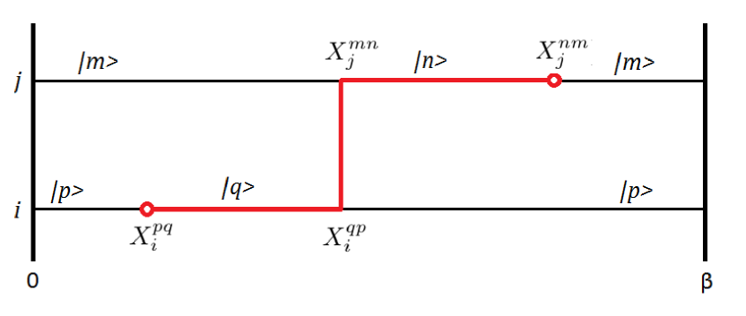
a)

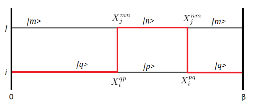
b)

Figure 1: The fragments of typical configurations. Panels show configurations with (a) and without (b) a worm. In the panel (a), the red color indicates the worldline of the worm; in the panel (b), the red color indicates the loop formed by the worm closing.

In CTWL method, the expansion of the partition function comes in the form of the worldlines states in the imaginary time. It is convenient to rewrite the Hamiltonian in a form suitable for this method:

$$H_{t-J}=\sum_{i,p}E_{p}X_{i}^{pp}+\sum_{ij,pq}V_{ij}^{pq}X_{i}^{pp}X_{j}^{qq}+$$

$$+\sum_{ij,pqrs}T_{ij}^{pqrs}X_{i}^{pq}X_{j}^{rs}+\sum_{i,pq}\nu_{pq}(X_{i}^{pq}+X_{i}^{qp}),$$ (15)

where $E_{p}$ are the eigenvalues of the one-site part of the Hamiltonian (10)) whereas the $V_{ij}^{pq}$ are the energies of the diagonal interaction between the states $|p\rangle$ and $|q\rangle$ on sites $i$ and $j$, respectively. In this form, to each segment of the horizontal line that lies between $\tau_{1}$ and $\tau_{2}$ in state $|p\rangle$, there corresponds the multiplier $e^{-\beta(E_{p}+V)d\tau}$, where $V$ is the average energy of the diagonal interaction over all neighboring segments and $d\tau=\tau_{2}-\tau_{1}$ is the imaginary time interval of the segment.

To each kink (a segment of the vertical line in Fig.1) between sites $i$ and $j$ there corresponds the multiplier $T_{ij}^{pqmn}X_{i}^{pq}X_{j}^{mn}$, where $T_{ij}^{pqmn}$ are the energies of nondiagonal interaction that corresponds to the state change. Also, with respect to the worm algorithm, to each discontinuities there corresponds the multiplier $\nu_{pq}X_{i}^{pq}$ that represents the worm boundary, where $\nu_{pq}$ is the above introduced fictitious energy.

Fig.1 shows the fragments of a typical configuration occurring during the simulation. The update of the configurations occurs according to the Metropolis algorithmmetropolis involving finite number of updating procedures. Those updating procedures are described in detail in ctwl . However, to increase the convergence as well as to ensure the ergodicity of the algorithm, it must be also accompanied by certain additional prescriptions troyer .

The observables are measured in the following way:

$$\langle A\rangle:=\frac{\sum_{MC}\langle p|Ae^{-\beta H}|p\rangle}{\sum_{MC}1}$$ (16)

where $A$ is some operator. Unfortunately in the fermion system we are faced with the sign problem. This problem is connected with the appearance of the negative statistical weights during the calculation.

$$\langle A\rangle=\frac{\sum_{MC}\langle p|Ae^{-\beta H}|p\rangle sign(W)}{\sum_{MC}sign(W)}$$ (17)

As a result, the errors increase exponentially with decreasing temperature which rules out an acceptable accuracy at low temperatures. Finally, the adopted algorithm goes through the following steps:

(i) an initial configuration is generated. In fact, the initial configuration selection has no impact on the final result. All possible impacts of this choice are eliminated by thermalization.

(ii) possible updating procedures are chosen randomly. The probabilities of the procedures are not constants but rather depend on the worms and kinks presented in the current configuration. It also should be noted that every procedure has the inverse one. The probabilities of such procedures must be chosen according to those of the direct ones.

(iii) the site $i$ and times $\tau_{1}$ and $\tau_{2}$ are chosen according to the procedure. The site $i$ is chosen directly in case of the worm-dependent procedure and randomly otherwise. Moments of time are calculated in accordance to the probability density calculated for each case.

(iv)the probability $W$ of accepting new configuration is calculated. If $W>R$, where $R$ is a random number from the interval $[0,1]$, the new configuration is accepted. If the updating procedure is interrupted due to the impossibility of the updates, it corresponds to the case $W=0$. However, such interruptions are part of the statistics and they occur in accordance with the detail balance.

(v) in case the system has no worms regardless of the accepting of the new configuration, the statistics is supplemented by the new data and the procedure goes back to the step (ii), otherwise the procedure goes to the step (ii) without the data supplementing.

Furthermore, by the fact that the CPU time depends linearly on the lattice size and the average sign remains large enough, which helps to keep errors in acceptable limits, the simulation can be made at a relatively large lattice size. All numerical results were obtained for a $20\times 20$ lattice cluster with periodic boundary condition. However, this size is not enough to ensure that the finite-size effects have no significant effects on the result. To make these effects negligible the size of the lattice cluster should be extended to at least the $30\times 30$ one.

IV Results

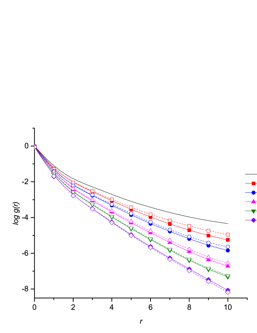
a)

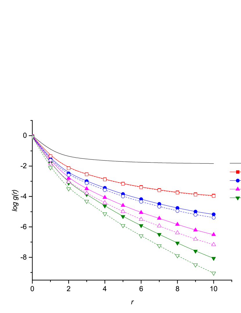
b)

Figure 2: Panel (a) and (b) show $\log g(r)$ for $J=0.2t$ (a) and $J=0.4t$ (b) with $T=0.1t$. Solid (dashed) lines show results obtained for $t^{\prime}=t^{\prime\prime}=0(t^{\prime}=-0.27t,t^{\prime\prime}=0.2t)$, respectively.

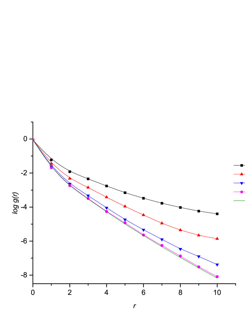
a)

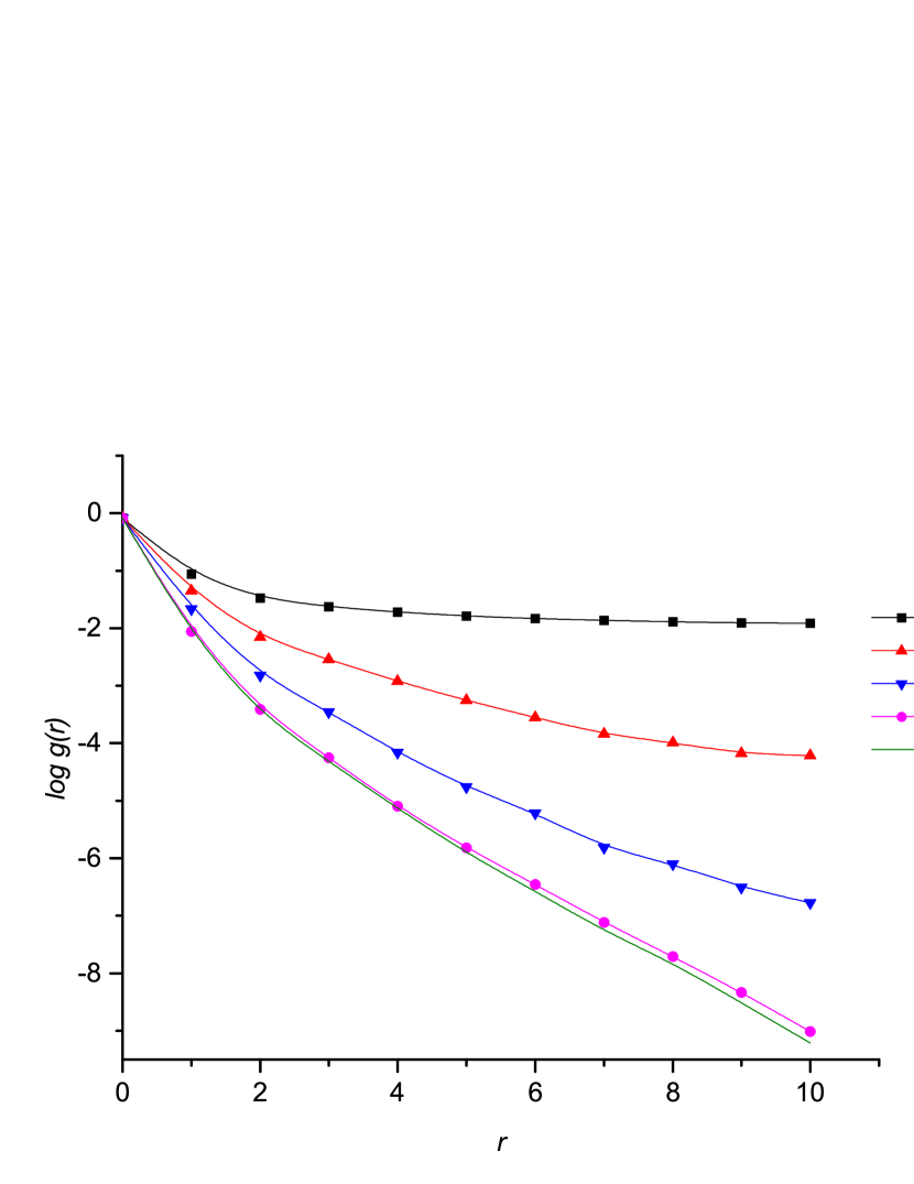
b)

Figure 3: Curves (a) and (b) show $\log g(r)$ for $J=0.2t$, $\delta=0.05$ (a) and $J=0.4t$, $\delta=0.08$ (b) with $T=0.1t$ and $t^{\prime}=-0.27t,t^{\prime\prime}=0.2t$.

To estimate the dependence of AF order from the doping level we compute the spin-spin correlation function $g(r)$ for the physical electron operators. This is calculated with $\sum_{i}{S_{i}^{z}}=\sum_{i}{s_{i}^{z}}=0$ and a fixed number of dopons, $\delta$:

$$\begin{gathered}g(r)=4\Delta^{-1}(r)\sum_{ij}\sum_{pq}\langle p|S^{z}_{i}+s^{z}_{i}|p\rangle\langle q|S^{z}_{j}+s^{z}_{j}|q\rangle\times\\ \times\langle X^{pp}_{i}X^{qq}_{j}\rangle e^{i\mathbf{K}\cdot(\mathbf{R}_{i}-\mathbf{R}_{j})}\bar{\delta}(r-|\mathbf{R}_{i}-\mathbf{R}_{j}|),\end{gathered}$$ (20)

where $\mathbf{K}=(\pi,\pi)$, $\mathbf{R}_{i}$ is radius-vector of the site $i$, $\Delta(r)=\sum_{ij}\bar{\delta}(r-|\mathbf{R}_{i}-\mathbf{R}_{j}|)$ and

$$\bar{\delta}(x)=\begin{cases}1&\text{if $|x|\leq 0.5a$,}\\ 0&\text{otherwise,}\end{cases}$$ (21)

with $a$ being the lattice constant and $\langle...\rangle$ means an average over the spin configurations generated in the QMC run. In all the figures showing $g(r)$ we use logarithmic scale for the vertical axis. Therefore, for the LRO, QLRO and SRO, the $g(r)$ should be represented asymptotically by a constant, a logarithmic function, and a straight line, respectively.

Fig.2 displays the electron spin-spin correlators for the different doping levels. The critical hole concentration varies from around $\delta_{c}=0.05$ at $J=0.2t$ to $\delta_{c}=0.08$ at $J=0.4t$. Due to a finite lattice size as well as a finite temperature a true long-range AF order manifest itself as a QLRO even at a very small doping. The suppression of the true LRO corresponds to the destruction of the QLRO due to the emergence of the short-range AF correlations. The obtained values of the critical hole concentrations do not necessarily coincide with the true ones to be computed at zero temperature in the thermodynamic limit. However their magnitudes are reasonably small.

In Fig.3 we report the spin-spin correlators, $\log g(r)$, for $J=0.2t$ and $J=0.4t$ at $\delta_{c}=0.05$ and $\delta_{c}=0.08$ for different values of $\lambda$, respectively. It is clearly seen that the QLRO is restored as $\lambda$ decreases. The local NDO constraint plays the dominating role in the destruction of the long-range AF state. At $\lambda>10t$, the spin-spin correlation functions become almost identical to each other. This indicates that finite but large enough values of $\lambda$ already provide a reliable description of the existing strong correlations. In this limit, the high and low energy itinerant fermions cannot be separated out and this is another manifestation of the duality of the lattice electron nature.

It should be noted that the physical meanings of the Kondo coupling $\lambda$ within the conventional phenomenological spin-fermion model chub and in our Eq.(7) are completely different. In the former case, it represents a SDW gap that can evolve from small to large values. In our theory, the only meaningful value of the Kondo coupling is that of $\lambda\gg t$ to take proper care of the NDO constraint.

V Conclusion

To conclude, we investigate the spin-spin correlation functions in the underdoped $t-J$ model numerically by employing quantum Monte Carlo simulations on finite clusters. Our main conclusion is that it is the local NDO constraint that is behind the rapid suppression of the AF QLRO at surprisingly small doping level. In contrast, any mean-field global treatment of the local NDO results in unphysically large values of the critical hole concentration.

The itinerant-localized duality of the lattice electrons offers the following explanation of the rapid destruction of the magnetic order by strong correlations. The localized individual lattice spins become less correlated with each other due to the competition between the AF correlations (the characteristic energy scale $\sim J$) and the Kondo screening ($\sim\lambda$) of the local spin moments by the conduction dopons. The screening breaks the AF bonds. In case a double occupancy is allowed, this breaking is not very efficient, as it is induced by the small (in this regime) spin-dopon interaction $\lambda$.

As $\lambda$ increases, the screening becomes more effective. Since $1/J\gg 1/t$, the hole dynamics is much faster than the spin one. The broken AF bonds recover themselves at a much slower rate than the breaking occurs. As a result, even a small amount of fast moving dopons (holes) turns out to be, at a large enough $\lambda$, sufficient to completely destroy the AF LRO.

A further possible application of the present approach might be that to theoretically explore an experimentally observed instability towards a formation of a charge order in the pseudogap phase at $\delta\approx 0.1$ There is a strong evidence that the observed charge order is due to strong electron correlations neto . The spin-dopon representation of the $t-J$ model provides a natural framework to address this problem. By varying $\lambda$, we would be able to vary the strength of the correlations to explicitly explore the impact of the NDO on the charge order formation. This is already in progress and results will be presented elsewhere.

VI Appendix

For the $1d$ $t-J$ model, the two leading terms of the ground-state energy expansion in powers of $J/t\ll 1$ are known explicitly. In the present Appendix, we show that the spin-dopon model (6) produces exactly the same result.

As the sign of $t$ is irrelevant, we can fix the Hamiltonian (6) in $1d$ to take the form

$$H_{t-J}=H_{J=0}+H_{int},$$ (22)

where

$$H_{J=0} =: H_{0}=-2t\sum_{ij\sigma}{d}_{i\sigma}^{\dagger}{d}_{j\sigma}$$ (23)

$$+ \frac{3\lambda}{4}\sum_{i\sigma}{d}_{i\sigma}^{\dagger}{d}_{i\sigma}+\lambda\sum_{i}\vec{S_{i}}\cdot\vec{s_{i}},\quad t>0,$$

and

$$H_{int}=J\sum_{ij}\vec{S}_{i}\vec{S}_{j}(1-n^{d}_{i})(1-n^{d}_{j}).$$ (24)

The limit $\lambda\to\infty$ reduces the local Hilbert space to that comprising a lattice spin-up state $|\uparrow\rangle_{i}=|\uparrow 0\rangle_{i}$, a spin-down state $|\uparrow\rangle_{i}=|\uparrow 0\rangle_{i}$ and a vacancy state $|0\rangle_{i}=\frac{|\uparrow\downarrow\rangle_{i}-|\downarrow\uparrow\rangle_{i}}{\sqrt{2}}$. We define the basis of the one-vacancy states as

$$|i,\{\sigma\}\rangle=|\sigma_{1}\sigma_{2}...0_{i}...\sigma_{N}\rangle,$$

where $\sigma_{k}=\uparrow\downarrow$ and $\{\sigma\}$ is a multi-index describing an arbitrary set of the lattice spins. The vacancy state $|0\rangle_{i}$ is a total spin singlet defined above.

The ground state at $J=0$ is degenerate with respect to spin. We can therefore choose a FM spin configuration. An arbitrary one-hole state is then given by

$$|\Phi\rangle=\sum_{i}\phi_{i}|i,\{\uparrow\}\rangle.$$ (25)

The energy of such a state is given by

$$\sum_{ij}\langle\Phi|H_{J=0}|\Phi\rangle=-\sum_{ij}t_{ij}\bar{\phi}_{j}\phi_{i}.$$ (26)

The corresponding Schrodinger equation reads

$$\sum_{j}(t_{ij}-E\delta_{ij})\phi_{j}=0.$$ (27)

The lowest-energy solution for the nearest-neighbour (nn) interaction reads

$$\phi_{j}=1/\sqrt{N_{s}},\quad E_{0}=-2t,$$

with $N_{s}$ being a total number of the lattice sites.

To consider a state with $N$ holes one should generalize Eq.(25) to include $N$ fermionic (hole) states:

$$|\Phi_{N}\rangle=\sum_{i_{1},i_{2},...,i_{N}}\phi_{i_{1},i_{2},...,i_{N}}|i_{1},i_{2},...,i_{N}\{\uparrow\}\rangle,$$

where the function $\phi_{i_{1},i_{2},...,i_{N}}$ is antisymmetric with respect to the index permutation. A corresponding Schrodinger $N$-particle equation can be then written out explicitly. Alternatively, one can quantize Eq.(27) with exactly the same effect. Namely, the $c$-valued amplitudes $\phi_{i}$ are replaced by the fermion operators

$$\phi_{i}\to\hat{\phi}_{i}=:f_{i},\quad[f_{i}^{+},f_{j}]_{+}=\delta_{ij}.$$

The $N$-hole generalization of the Hamiltonian $H_{0}$ then reads

$$H_{0}=-\sum_{ij}t_{ij}f^{+}_{i}f_{j},\quad\sum_{i}f_{i}^{\dagger}f_{i}=N.$$ (28)

This Hamiltonian describes spinless fermions hopping in a $1d$ lattice. In case of the nn interaction, the ground-state energy becomes

$$E_{0}=-\frac{2t}{\pi}\sin(\pi\delta),\quad\delta=\frac{N}{N_{s}}=\frac{1}{N_{s}}\langle\sum_{i}f^{+}_{i}f_{i}\rangle_{H_{0}}.$$

The spin degeneracy is lifted by the effective spin-spin interaction:

$$H_{t-J}^{gr}=-\frac{2t}{\pi}\sin(\pi\delta)+J_{eff}\sum_{ij}\vec{S}_{i}\vec{S}_{j}+{\cal O}(J^{2}),\quad J\to 0.$$ (29)

We have

$$J_{eff}=J\langle(1-f^{\dagger}_{i}f_{i})(1-f^{\dagger}_{j}f_{j})\rangle_{H_{0}}$$

$$=J((1-\delta)^{2}-\frac{\sin^{2}\pi(1-\delta)}{\pi^{2}}).$$

In terms of the electron density $n_{e}=1-\delta$, Eq.(29) becomes

$$H_{t-J}^{gr} = -\frac{2t}{\pi}\sin(\pi n_{e})$$ (30)

$$+ J(n_{e}^{2}-\frac{\sin^{2}\pi n_{e}}{\pi^{2}})\sum_{ij}\vec{S}_{i}\vec{S}_{j}+{\cal O}(J^{2}),$$

which agrees with the Bethe-ansatz result obtained for the canonical $t-J$ model given by Eq.(1)shiba .

References

- (1) See, e.g., P.A. Lee, N. Nagaosa, and X.-G. Wen, Rev. Mod. Phys. 78, 17 (2006), and references therein.
- (2) A. Ferraz, E. Kochetov, and B. Uchoa, Phys. Rev. Lett. 98, 069701 (2007); R.C. Pepino, A. Ferraz, and E. Kochetov, Phys. Rev. B 77, 035130 (2008).
- (3) M.M. Maska, M. Mierzejewski, A. Ferraz, and E.A. Kochetov, J. Phys. Condens. Matter 21, 045703 (2009); M.M. Maska, M. Mierzejewski, and E.A. Kochetov, Phil. Mag. 95, 583 (2015).
- (4) T.C. Ribeiro and X.-G. Wen, Phys. Rev. Lett. 95, 057001 (2005); T.C. Ribeiro and X.-G. Wen, Phys. Rev. B 74, 155113 (2006).
- (5) A. Ferraz, and E. Kochetov, Eur. Phys. J. B 86, 512 (2013).
- (6) Ar. Abanov, A.V. Chubukov, J. Schmalian, Adv. Phys. 52, 119 (2003).
- (7) Eduardo H. da Silva Neto, et.al., Science 343, 393 (2014).
- (8) N.V. Prokofev, B.V. Svistunov, and I.S. Tupitsyn, JETP, 114, 570 (1998).
- (9) N.V. Prokofev, B.V. Svistunov, and I.S. Tupitsyn, Phys. Lett. A, 238, 253 (1998).
- (10) M. Troyer, F. Alet, S. Trebst, S. Wessel, AIP Conf. Proc. 690, 156 (2003).
- (11) N. Metropolis et al., J. Chem. Phys., 21, 1087 (1953).
- (12) H. Shiba and M. Ogata, Int. J. Mod. Phys. B5, 31 (1991).